Lessons
Lesson 1
Overview
Did you complete the Course Orientation?
Before you begin this course, make sure you have completed the Course Orientation [1].

About Lesson 1
Most of us do not notice the daily and yearly changes in the sky because, frankly, we no longer have to bother! Clocks and watches have been around so long that they hardly seem to be advanced technology. Anyone can look at a calendar to tell you what the date is, and, if we are lost on an unfamiliar road, most phones have GPS functions that can help us find our way home. Even though calendars, clocks, and navigational tools have insulated us from the need to understand the motions of the sky, most of us do appreciate that our system of time and our location on the surface of the Earth can be tied directly to observations of the sky.
In this lesson, we will study the observable changes in the positions of objects in the sky and show how these data allow us to understand the relative positions and motions of the Sun, Moon, Earth, and the stars. My hope is that from this point forward, whenever you look at the sky you'll be aware of what it can tell you about time, date, and your location.
What will we learn in Lesson 1?
By the end of Lesson 1, you should be able to:
- identify the objects visible in the night sky to the unaided eye;
- describe the three dimensional geometry of the Earth / Moon / Sun system;
- describe the various motions in the sky that result from Earth’s rotation and orbit;
- explain the reason that the Earth experiences seasons;
- describe the process and appearance of eclipses and the phases of the Moon.
What is due for Lesson 1?
Lesson 1 will take us one week to complete. Please refer to the Calendar in Canvas for specific time frames and due dates.
There are a number of required activities in this lesson. The following table provides an overview of those activities that must be submitted for Lesson 1.
| Requirement | Submitting Your Work |
|---|---|
| Lesson 1 Quiz | Your score on this Canvas quiz will count towards your overall quiz average. |
| Discussion: Teaching and Learning about the Moon | Participate in the Canvas discussion forum "Teaching and Learning About the Moon." |
Questions?
If you have any questions, please post them to the General Questions and Discussion forum (not email). I will check that discussion forum daily to respond. While you are there, feel free to post your own responses if you, too, are able to help out a classmate.
Definitions
If you want to complete some additional reading beyond what is in our Lesson 1 pages, I recommend:
In this lesson, we will be using some vocabulary that may be either unfamiliar or may be used differently, in an astronomical context, from your usual usage. Normally, I advocate for discussing vocabulary in the context of a lesson, instead of presenting it like this to begin the lesson. In our case, though, I'm going to break my own rule so that we can start discussing the sky immediately and make sure that we agree on the meaning of these terms. The vocabulary you will encounter in this lesson includes:
- Altitude
- Azimuth
- Meridian (and transit of the meridian)
- Horizon
- Zenith
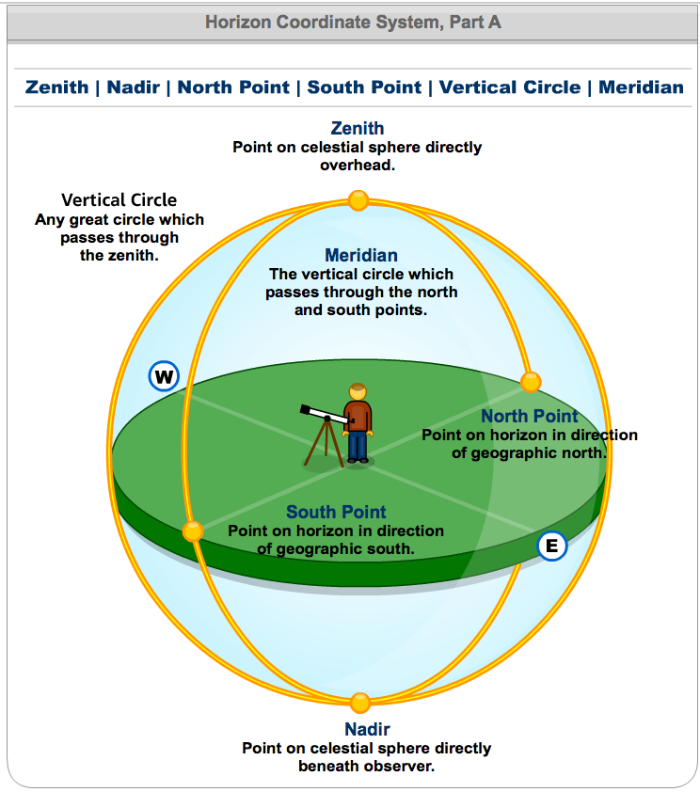
All of these terms are used to describe the location or behavior of objects in the sky. For example, you can refer to the altitude of the Sun. Or, when the Sun passes from one side of the meridian to the other, you can talk about the Sun "transiting the meridian." These terms and their meanings are illustrated using the following two diagrams. Read over the list of terms and definitions in the list and/or mouse over the terms in the image to view their definitions.
Horizon Coordinate System, Part A
- Zenith - Point on celestial sphere directly overhead.
- Nadir - Point on celestial sphere directly beneath observer.
- North Point - Point on horizon in direction of geographical north.
- South Point - Point on horizon in direction of geographical south.
- Vertical Circle - Any great circle which passes through the zenith.
- Meridian - The vertical circle which passes through the north and south points.
Horizon Coordinate System, Part B
- Altitude - The angular distance from horizon to object, measured along a vertical circle.
- Azimuth - The angular distance along horizon from N (S) eastwards to vertical circle through object (for Northern (Southern) hemisphere.

Day and Night
Additional Reading at www.astronomynotes.com: [6]
The most obvious change in the sky is that for about half of the day the sky is brightly lit and, for the other half, it is dark. If the sky is clear, we can tell that the Sun is “up” during the day and “down” at night. Even though this is obvious to most observers, there is one question about day and night that took many centuries to solve:
Is the Earth stationary and is the Sun orbiting it, or vice versa?
In the three movies above, we first see the motion of the Sun from East to West that we are familiar with seeing over the course of the daylight hours on one day. In the second movie, we see a stationary observer on a stationary Earth watching a moving Sun. This would reproduce what we see of the Sun appearing to move from east to west across our sky. The last movie shows another alternative; the Sun is at a stationary location from our perspective, and the Earth is rotating, causing the Sun to appear to move.
We will discuss some of the history of this question (which is a very interesting discussion of the history of astronomy) in Lesson 2, but for now I will directly answer the question.
The Earth rotates around an imaginary line that goes through the North and South Poles, which is called the axis of rotation.
This movie shows the rotation of the Earth along the axis that goes through the North and South poles.
One can make a representation of how the rotation of the Earth makes the Sun appear to move across the sky kinesthetically: If an object is at a fixed location on a wall (for example, a clock) and I am facing it, then I can see the clock. If I rotate so that I'm facing away from the clock, I can no longer see it. While I am rotating, the clock will, from my point of view, appear to be moving. You can try this out wherever you are right now!
If the Sun is in a "fixed" location on the sky and the Earth is facing this location, then we can see it (daytime!). When the Earth has rotated by 180 degrees, we are no longer facing the Sun, so we can't see the Sun (nighttime!). From our point of view fixed to a specific location on the Earth, as the Earth rotates it is the Sun that appears to move, just like the clock in my example above. This is our modern understanding of day and night.
This has consequences beyond day and night. The Earth's rotation causes every object in the sky to appear to trace out a path on the sky from East to West. So if you pick out a star in the sky, it will appear to make an arc across the sky. This is because, for our purposes, we can consider the star to be fixed in space, and the Earth is rotating underneath it. This happens slowly, so from minute to minute you don't notice the star's motion. However, over the course of a few hours you will be able to tell that the stars have moved a substantial distance on the sky. Since, like the Sun, the stars will (for the most part) appear to rise in the east and set in the west, so the apparent motion of a star will depend on which direction you face. An example follows in a 3 second movie. In the top left panel, you see stars appear to rotate counterclockwise around the North Celestial Pole, which is what we would see if facing north. In the top right panel, you see stars rising in the east, moving along circular, clockwise paths, and setting in the west, which is the behavior we would see if facing south. The lower panel shows the stars rising diagonally from the east on the first part of this circular path, which is what we would see if facing east.
Reproducing the above animation with real observations of the stars is a popular type of astrophotography. An example is an image following of the apparent motion of the stars across the sky as seen from Mt. Kilimanjaro.

The picture was created by leaving the camera shutter open for more than three hours (Note: can you tell how long the exposure was? How might you figure this out?), so it shows the path the stars in the sky follow over a small fraction of the night. This image also illustrates another important point—the Sun and the stars all appear to rotate around one point, which is the point directly above the North Pole of the Earth for observers in the northern hemisphere (called the North Celestial Pole or NCP), or the point directly above the South Pole of the Earth (the South Celestial Pole or SCP) for observers in the southern hemisphere. There is a star that is positioned very close to the NCP, which is called Polaris, the Pole Star. It is NOT the brightest star in the sky; it isn't even in the top 25. The importance of Polaris is that it roughly marks the location of the NCP, so all stars visible to observers in the northern hemisphere appear to rotate around Polaris.
Test this with Starry Night!
- Open up Starry Night.
- Using the bar at the top, set the time to a time after Sunset, say 9:00 p.m.
- Set the time flow rate to 300x.
- Face South (if you aren't already, type "S").
- Press the play button, and watch the stars move on the sky from 9:00 p.m. - 11:00 p.m.
- Reset to 9:00 p.m. and then do the same, but facing East and then West. How did the motion of the stars differ?
We can prove to ourselves that the apparent motion of objects in the sky depends on your location on the Earth! For example, consider the following cases:
- If you are standing at the north pole, Polaris will be directly overhead. From your point of view, all stars will appear to make horizontal, circular paths around your zenith.
- If you were standing on the Earth’s equator (say near Mt. Kilimanjaro, as in the image linked above), you would have to look due North towards your horizon to find Polaris, so the stars would appear to rise almost vertically from the eastern horizon, and the point around which they appear to rotate is near or at the northern horizon.
- If you are in between the equator and the north or south poles (say in State College, PA), the point around which all the objects appear to rotate is about midway between your horizon and the zenith (at an altitude equal to your latitude, approximately 40 degrees).
Note that for observers at most locations above or below the equator, there are some stars that are near the NCP, and these trace out small circular paths that are never below the horizon. These stars that never rise or set are called circumpolar stars. The lower the altitude Polaris appears from your viewing location (that is, the closer your latitude is to that of the equator), the fewer the number of stars that are circumpolar from your point of view.
Test this with Starry Night!
- Open up Starry Night.
- Change your location to the North Pole. (Set the location to a latitude to 90 degrees North)
- Set the time to 9:00 p.m. If the sky appears to be light, you can momentarily turn off the Sun: Under the View menu or using the Display Optios you can select "Hide Daylight," which will allow you to see the stars even when the Sun is up.
- Set the time flow to 300x.
- Press the play button and watch the stars move on the sky. How many stars are circumpolar here?
- Do the same for the Equator (Latitude 0 degrees).
- Face North, South, East, and West and watch the stars move on the sky. How many stars are circumpolar here?
- How did the motion of the stars differ at the Equator compared to near the North Pole? Can you make a sketch to explain why the stars appear to move differently at these locations? It might be helpful to think about the how one's horizon at a particular location on the Earth, relative to Earth's rotation axis, limits their view of the sky.
The Path of the Sun
Additional Reading at www.astronomynotes.com: [6]
During the day, we can see the Sun, but the bright daylight sky prevents us from seeing most other objects in the sky (on some days you can see the Moon during the day, and if you know where to look you can also sometimes see Venus).
As a thought experiment, think about what you might see if you were able to see the Sun and the stars in the sky during the daytime simultaneously.
- What stars would you see behind the Sun?
- Would you always see the same stars behind the Sun?
Test this with Starry Night!
- Open up Starry Night, set it for Sunrise, and set the time flow rate to 1 hour.
- Under the View menu or using the options tab, you can select "Hide Daylight," which will allow you to see the stars even when the Sun is up.
- If you want, to help guide your eye, you can also turn on the constellation stick figures using the View menu, the Options tab, or just by typing the letter "k" on the keyboard.
- Now, step through time one hour at a time by hitting the step forward button. Take note of the Sun's path and its position with respect to the stars.
Let's look at two movies made with Starry Night. The first illustrates the path of the Sun during one day (Sunrise to Sunset), following the instructions listed prior.
The second illustrates the position of the Sun at noon eastern on June 21, September 21, December 21, and March 21.
If you could see the Sun and the stars simultaneously, you would see that during the course of one day, the Sun would be inside one constellation (to be more specific, one of the constellations of the Zodiac). To be even more specific, realize that the constellations are made up of stars far in the background, so when we say the Sun is "inside" a constellation, we mean that we are seeing the Sun in projection in front of a specific group of distant stars.
In the first of the two movies, notice the Sun's position relative to the constellation Virgo at 7:00 AM, noon and 6:00 PM. As we discussed at the beginning of the lesson, it is the rotation of the Earth that causes the Sun and the stars to move across the sky, so we should expect that the Sun and the stars should both appear to move at the same rate. Thus, the Sun will be seen inside of the same constellation during the entire day. That is, if the Sun appears to be in the constellation of Gemini at dawn, then it will still be in Gemini at noon and at Sunset.
This is mostly correct, however, there is one effect that we are neglecting to take into consideration. The Earth isn’t just rotating in a fixed spot in space. The Earth is also orbiting around the Sun. In one year, the Earth will make a complete trip around the Sun. So, in December, the Earth will be on one side of the Sun, and six months later, in June, it will be on the opposite side of the Sun.
The second Starry Night movie shown above demonstrates that in December, when the Earth is facing the Sun, the constellation behind the Sun is Sagittarius. Twelve hours later, when the Earth has rotated so that it is night, the Earth is facing directly away from the Sun, towards the constellation of Gemini. In June, the situation is completely reversed because the Earth is on the opposite side of the Sun. The constellation behind the Sun at noon in June is Gemini, and twelve hours later, when the Earth is facing directly away from the Sun, it is pointed towards the constellation of Sagittarius.
This is reasonably easy to visualize when you think of the extreme case of the differences in the position of the Earth six months apart, but what happens on a day to day basis? The way to visualize it is as follows. The stars are so far away from the Earth that, again, for our purposes, we can consider them to be fixed. We know that the rotation of the Earth causes stars to appear to make circles or arcs on the sky that start in the east and move westward. A natural question to ask is, “How long does it take for star A to appear in the same spot in the sky one day later?” That is, let’s say that star A is “transiting your meridian” (this means that if you draw the imaginary line on the sky that connects due North to due South, the star is passing this line at this particular instant in time), how long will it be until star A transits your meridian the next time? You may be tempted to say 24 hours, but the correct answer is 23 hours and 56 minutes! If you do the same exercise for the Sun—that is, if you calculate the time between successive transits of the Sun—it is 24 hours (although it does vary over the course of the year, and some days are slightly longer and others are slightly shorter than 24 hours).
The length of time between transits for a star (any star) is called a Sidereal Day, and the length of time between transits for the Sun is called a Solar Day. The difference is caused by the slow drift of the Earth around the Sun. Because the Earth has moved 1/365th of the way around the Sun in a day, it has to rotate more than 360 degrees in order for the Sun to appear in the same part of the sky (e.g., transiting the meridian) as it did yesterday. However, since the stars are so far away, the Earth’s orbit around the Sun doesn’t affect their apparent position in the sky, so the Earth only needs to rotate 360 degrees in order for them to appear in the same part of the sky. Because of this effect, the Sun appears to slowly drift eastward compared to the background stars, and the cumulative effect of this drift is that the Sun will appear to be in Gemini in June and Sagittarius in December.

Note in the figure above that when the Earth rotates 360 degrees, it goes from position 1 to position 2, and a distant star will appear to be in the same position as seen from Earth. However, the Earth has to go from position 1 to position 3 for the Sun to appear in the same position.
Test this with Starry Night!
- Open up Starry Night, and set it for a time when it is completely dark, say 11:00 PM.
- Using the View menu turn on the Local Meridian line.
- Either adjust the time slightly or let time flow forward until a bright star is on the meridian.
- Now, from the time flow rate box, select "days" as the time step.
- If you click on the forward button, you should see that each day at the same time, your bright star that started on the meridian will get further and further from the meridian.
- Next, click the backward button so that the bright star is back on the meridian.
- Now, change the time step to be "sidereal days."
- Now, if you click the forward button, your star should remain on the meridian without moving each time you click.
The Height of the Sun
Additional Reading at www.astronomynotes.com: [6]
- Astronomy without a telescope [3]
- Seasons [12]
We are still not done talking about the apparent changes of the Sun in the sky. You now know that the Sun appears to move from east to west because of the rotation of the Earth, and that if you could see the stars during the daytime it would appear to drift with respect to the stars by a small amount each day because of the orbit of the Earth around the Sun. The next question is:
Does the apparent path of the Sun across the sky change during the year?
Again, let’s consider two extreme cases—December and June. Think about the appearance of the Sun in winter and then in summer. If you live at roughly the same latitude as central Pennsylvania, you should remember that the Sun never gets very high above the horizon in December, but in June it passes almost (but not quite!) directly overhead. So, the apparent path of the Sun does change from season to season. You can also observe this effect if you re-run the animation on the previous page; in June, the Sun is high above the horizon, in September it is lower, and in December it is very low on the horizon.
The cause of this effect is that the axis of the Earth’s rotation (the imaginary line that passes from the North Pole through the Earth to the South Pole) is tilted with respect to the Sun by an angle of 23.5 degrees. If you go back and look at the animation of the rotating Earth on the day and night page in this lesson, you will see that the line indicating the axis of rotation is not vertical, but is offset by 23.5 degrees from the vertical. As the Earth orbits the Sun, the orientation of the Earth stays fixed, and as a result, in December, the northern hemisphere is tilted away from the Sun during the day, and in June the northern hemisphere is tilted towards the Sun during the day.
There are two consequences of the tilt of the Earth’s rotation axis:
- When the hemisphere you are located on is tilted towards the Sun, the path of the Sun across the sky will be longer than when the hemisphere you are on is tilted away from the Sun. That is, there are more hours of daylight during summer than there are during winter.
- When the hemisphere you are located on is tilted towards the Sun, the light from the Sun is hitting the Earth more directly where you are located than when the Earth is tilted away from the Sun. This means more energy is hitting each square meter of Earth during summer than winter, making summer days hotter than winter days.
Try This!
To help visualize this, you can do a simple demonstration if you have a desktop globe and a lamp with a bare bulb. Most globes are set with their axis of rotation set to 23.5 degrees from vertical. In a dark room, place the globe on a table so that the northern hemisphere is tilted towards the lit lamp, which represents the Sun. You should see that if you pick out a spot, say Pennsylvania, and then watch that spot as you spin the globe, Pennsylvania will get light from the lamp for about 2/3 of its path as it rotates on the globe. If you now move the globe to the other side of the lamp (that is, the northern hemisphere should now be pointing away from the lit lamp), this simulates Earth's position six months later. If you again pick out Pennsylvania on the globe and watch it as it spins, it will receive light from the lamp for only about 1/3 of its path as it rotates on the globe.
Note that the tilt of the Earth is neither towards nor away from the Sun during March and September (Spring and Autumn). Thus, the path of the Sun across the sky and the angle of the Sun’s rays is similar during these two seasons, which is why the length of the day and the daytime temperatures are similar.
There is a nice animated demo from PBS that helps illustrate this effect: Cycles in the Sky: Crash Course Astronomy #3 [13].
Recall that the ecliptic is the path of the Sun across the sky; it can be represented by an imaginary circle in space. If we take the Earth’s equator (another imaginary circle) and project it on the sky, the angle between the ecliptic and the celestial equator would be 23.5 degrees because of the tilt of the Earth. Because the tilt of Earth's rotation axis gives rise to the angle between the ecliptic and the celestial equator, astronomers refer to the tilt of Earth's rotation axis as the "obliquity of the ecliptic". There are four special points on the ecliptic (and note that since the ecliptic is the same thing as the path of the Earth around the Sun, points on the ecliptic are the same things as dates on our calendar):
- Equinoxes - The equinoxes are the two points on the ecliptic where it crosses the celestial equator. On the vernal and autumnal equinoxes (around March 21 and September 21 respectively) the length of the day and night are roughly (but not exactly!) equal.
- Solstices - The points on the ecliptic when the Sun is highest above or lowest below the celestial equator are called the solstices. On the winter solstice (around December 21 in the Northern Hemisphere), the night is much longer than the day, and on the summer solstice (around June 21 in the Northern Hemisphere), the day is much longer than the night. See the three figures below for a comparison between the celestial equator (red line) and the ecliptic (green line):


So, why do we experience seasons?
This emphasizes one major point that is the most misunderstood fact in astronomy:
The Earth experiences seasons because of the tilt of its axis of rotation. The seasons have nothing to do with the distance of the Earth from the Sun.
There is one observation that should help you remember the cause for the seasons. The seasons are opposite in the northern and southern hemispheres on the Earth. That is, it is summer in Pennsylvania from June through September, but in South Africa, it is wintertime during these same months! This is easy to explain if you understand that the Earth’s tilt causes the seasons; when the northern hemisphere is tilted towards the Sun (summertime), the southern hemisphere is tilted away from the Sun. If the distance between the Earth and the Sun caused the seasons, then it would have to be summer in both the northern and southern hemispheres at the same time, because both would be the same distance from the Sun at the same time. Do you know when the Earth is closest to the Sun? In January!
Often, when confronted with the understanding that it is the tilt of the Earth's rotation axis that causes the seasons, students who feel strongly that the reason the seasons must be a difference in distance from the Earth to the Sun will point out that the hemisphere tilted towards the Sun is now closer to the Sun. However, the Earth is so far from the Sun that the difference in distance to the Sun between the hemisphere tilted towards the Sun and the one tilted away from the Sun is effectively zero.
The Phases of the Moon
Additional Reading at www.astronomynotes.com: [6]
The changing Moon is a familiar sight to all of us, since it is the second brightest object in the sky after the Sun. The images of the Moon below were created by taking images of the Moon over approximately one month.

Looking more closely at these images, you can notice a few characteristics in the appearance of the Moon:
- It always keeps the same face pointed towards the Earth.
- It goes from completely dark to completely illuminated and back again.
Let’s start with the phases. First, we need to again talk about the layout of the Sun, Earth, and Moon system. We already have learned that the Earth is orbiting the Sun, and it is rotating on its tilted axis as it orbits. At the same time, the Moon is orbiting the Earth, and as it orbits around the Earth, it is rotating, too. Just like the Earth, the half of the Moon that is pointed towards the Sun is illuminated, and the half of the Moon that points away from the Sun is dark. So, the simple explanation for the phases of the Moon is that, at any one time, half of the Moon is light and half is dark, and the appearance of the half of the Moon that we see changes as it orbits the Earth. For a listing of the individual phases and a description of their appearance, see "Phases of the Moon and Percent of the Moon Illuminated. [16]"
Try This!
For this lesson, we begin by referring to the following animation. Note that the animation is 6 minutes, 4 seconds long, and that there is much to interpret.
Once the movie begins, you should see that the Earth begins to rotate and the Moon begins to orbit the Earth. The Moon is also rotating, but that is less obvious (we will discuss this more later). Please keep this animation in mind when we discuss the phases—remember that all of these phenomena happen simultaneously (Earth's rotation and orbit, Moon's rotation and orbit).
Next visit Lunar Phase Simulator [17] developed by the University of Nebraska-Lincoln. This is an image that requires some interpretation, but if you can figure it out, you will have mastered an understanding of the phases of the Moon. The Sun is far off to the left on the diagram, so sunlight is illuminating the left side of both the Earth and the Moon. The point on the Earth immediately underneath the Sun experiences noon, and if you imagine the stationary Earth in the diagram rotating counterclockwise, that point will experience sunset when the Earth has rotated 1/4 of the way around, then midnight, then sunrise, then back to noon. Those times are labeled.
In the same diagram, the Moon is shown in eight different locations along its orbit around the Earth. For example, the full Moon occurs when the Sun, Earth, and Moon are in a line in that order (labeled as position 4). The sunlight that is hitting the Moon illuminates the half of the Moon that points towards the Earth. So, when the Moon is full, its entire illuminated half is pointed directly at the Earth.
The next question that you can answer from this diagram is: What time is the full Moon visible on Earth? To answer this question, we can integrate our knowledge about the rotation of the Earth. Picture yourself on the daylight part of the Earth pointing directly at the Sun. Remember, it is noon for you when you are on the part of the Earth pointing directly at the Sun, which is when the Sun is transiting your meridian. Six hours later, when the Earth has rotated one quarter of the way around, you would have to look to the western horizon to see the Sun, and to the eastern horizon to see the Full Moon. So, at sunset (about 6:00 PM), the full Moon is rising. Six hours later, the Earth has rotated an additional one quarter of the way around. Now, the Moon is directly in front of you (that is, this time it is transiting your meridian). So, the full Moon transits at midnight. Six hours later, at about 6:00 AM, the Moon will now be on your western horizon (setting), and the Sun will be on the eastern horizon (rising).
The New Moon phase occurs when the Sun, Moon, and Earth are in a line in that order (unlabeled, but it is position 8). In this case, the unilluminated side of the Moon faces the Earth. Thus, during New Moon, we do not see the Moon in our sky at all. Using the logic from the paragraph above, even though we can't directly see the New Moon, we know that the New Moon transits at 12 PM (noon), sets at sunset (about 6 PM), and rises at sunrise (6 AM).
The other phases fall in between these two extremes. For example, at First Quarter, the side of the Moon facing the Earth is half illuminated and half dark. It will rise at noon, transit at 6 PM, and set at midnight.
Let's end this discussion of the Moon by returning to its rotation. If the Moon rotates, why does it always show the same face to the Earth? Shouldn’t we see the face of the Moon slowly changing as it rotates? For example, think about observing the Earth from the point of view of the Sun; during the course of 24 hours, you will see North America rotate out of your view and then back again. We will discuss this in more detail in a later lesson, but the short answer is that the Moon’s rotation rate is matched to its orbital rate. That is, the Moon takes the same amount of time to rotate as it takes to orbit. Because of this, it keeps the same face pointed towards the Earth at all times.
The last point to make about the phases is the time it takes for the Moon to complete one complete cycle of phases. We know that the length of our day is tied to the rotation rate of the Earth and the length of our year is tied to the orbital period of the Earth around the Sun, so what about the Moon? Well, it takes approximately 29.5 days for the Moon to complete one set of phases, or roughly one month.
Eclipses
Unlike day and night, the phases of the Moon, and the seasons, this last phenomenon is a rare event that you may or may not have personally experienced or listed on your set of observations. This may have just changed as of August, 2017, as many of us got to experience the solar eclipse that passed through much of the US [18]! Eclipses occur infrequently because they require a very specific alignment of the Sun, Earth, and Moon. If the Moon is lined up precisely with the Sun from the Earth’s point of view, the Moon will block Sunlight from reaching the Earth, causing a solar eclipse. If the Moon is on the other side of the Earth from the Sun, the Earth will block Sunlight from reaching the Moon, causing a lunar eclipse. According to the diagram of the Moon phases from the Lunar Cycles module, it appears that the Sun, Earth, and Moon are lined up for an eclipse twice a month!
Is there a solar eclipse every new Moon and a lunar eclipse every full Moon?
As it turns out, there is another effect that we need to account for. In order for there to be an eclipse during every full Moon and new Moon, the orbital plane of the Moon around the Earth would have to be identical to the orbital plane of the Earth around the Sun. That is, the three objects have to be precisely lined up as in the first diagram below. If, for example, the Moon is above or below the Earth’s shadow, there will not be a lunar eclipse. Similarly, if the Moon’s shadow does not hit the Earth because the Moon is above or below the plane of the Earth’s orbit around the Sun, there will not be a solar eclipse. The plane of the Moon’s orbit is inclined by 5 degrees compared to the plane of the Earth’s orbit, so at most times the Moon is above or below the position necessary to cause an eclipse.
If you think of the Earth’s orbit around the Sun as a disk and the Moon’s orbit around the Earth as another disk, there is a 5 degree angle between the two disks. However, any time you have two circles that intersect each other like the two disks do, there will be two points at which the intersection occurs (just like the two equinoxes we discussed above are the two points where the Celestial Equator and Ecliptic intersect). These two points on the Moon’s orbit (where the Moon lies in the same plane as the Earth’s orbit) are called nodes, and the line connecting these two points is called the line of nodes.
So, the recipe for having a solar or lunar eclipse requires two circumstances, not just one. They are:
- The phase of the Moon must be new for a solar eclipse or full for a lunar eclipse to occur (top figure).
and - The line of nodes must be closely aligned with the Sun and the Earth (bottom figure).


Watch This!
You can find a brief video clip about a solar eclipse [19] at the Teachers' Domain website.
NOTE: "Teacher's Domain" is a free resource, but you must register with them in order to view more than 7 resources. Since we'll point to that resource throughout this course, you may want to take a moment to go ahead and register with them now.
The appearance of the Sun and Moon during eclipses
Finally, let’s conclude this lesson with a discussion of how the Sun and Moon appear during eclipses. There are three possibilities for a lunar eclipse, depending on how well the line of nodes is aligned with the Sun and Earth:
- Total Lunar Eclipse: Occurs when the Moon is entirely contained within the Earth’s umbra.
- Partial Lunar Eclipse: Occurs when the Moon is partly in the umbra of the Earth and partly in the penumbra.
- Penumbral Lunar Eclipse: Occurs when the Moon is entirely contained within the penumbra.
During a total lunar eclipse, the Moon will darken considerably and glow red as the Earth allows some of the red light from the Sun to reach the Moon. During a partial lunar eclipse, part of the Moon will appear darker and redder, while the rest will appear normal. Most of us don’t even notice penumbral lunar eclipses, because the Moon only dims.
Here are some examples:
- Astronomy Picture of the Day: 2003 November 21 [20]
- Astronomy Picture of the Day: 2001 January 18 [21]
- Astronomy Picture of the Day: 2003 May 22 [22]
One significant difference between solar and lunar eclipses that we must mention is that a solar eclipse is only visible to certain parts of the Earth. See these Astronomy Pictures of the Day to see why:
- Astronomy Picture of the Day: August 30, 1999 [23]
- Astronomy Picture of the Day: 2002 December 9 [24]
There are three types of solar eclipses, too:
- Total Solar Eclipse: Anyone on Earth who lives in an area where the Moon’s umbra passes will see the entire Sun obscured by the Moon. For example: Astronomy Picture of the Day: 2002 December 6 [25]. Many of you have probably heard this, but people who have experienced a total solar eclipse describe it as one of the most breathtaking phenomena in their lives. It is almost impossible to capture in images or videos the effects, but there are a number of very interesting aspects of total solar eclipses that awe the people who see them. For example, here is an image of the "Diamond Ring" [26] effect just after totality during the August 21, 2017 eclipse. The next total solar eclipse that will be visible in the US is in April of 2024. Here is a Google map [27] of the eclipse path. This course's author stayed in PA for the 2017 eclipse, but will be traveling to the path of totality for the 2024 eclipse and encourages all of you to do the same!
- Partial Solar Eclipse: If you live just outside the path of the Moon’s umbra, but within the path of the Moon’s penumbra, you will see part of the Sun obscured by the Moon. Here is a good example: Astronomy Picture of the Day: September 3, 1997 [28]. There are many images like this from the August 2017 eclipse.
- Annular Solar Eclipse: Recall from the movie of the lunation above that the Moon appears to be a little bit bigger sometimes and a little bit smaller other times. This is caused by the Moon’s elliptical orbit. Sometimes it is closer to the Earth than other times. Well, if the Moon just happens to be in a position that is slightly farther from Earth, it won’t completely cover the Sun even during a total solar eclipse. In this case, you see a ring of the Sun still visible, such as in this example: Astronomy Picture of the Day: 2003 June 5 [29].
Additional Resources
On these pages, I will try to include links to resources specific to the content in the current lesson. However, since this is the first lesson, I'm going to put some general resources here that will be useful throughout the course.
- Perhaps my favorite astronomy website is Astronomy Picture of the Day [30] (APOD). I recommend visiting this site daily (or at least weekly) to see what the new image is and to read the caption that explains the image. Almost every image you see featured at APOD will be relevant to material you will learn at some point this semester. Here are a few of the APOD images I already linked to or that are related to the Lesson 1 material:
- An image of the star trails seen by an observer near the equator [31]
- An animation of a Lunation [32]
- An image of the Moon during a 2003 lunar eclipse [33]
- An image of the Sun's shadow on the Earth during a solar eclipse [34]
- An image of a 2008 solar eclipse [35]
Note that APOD has been in existence since June of 1995, so there are more than 8,000 images in their archive. If you are ever looking for an astronomical image of a specific object (e.g., M13 star cluster) or phenomenon (e.g., Sundog), their search feature is an excellent place to start. - For more imagery specifically from the Hubble Space Telescope, you can go to Hubblesite [36], which also has much more to explore beyond static images.
- My favorite group activity for teaching the 3D relationship between the Sun, Earth, and Moon is called "kinesthetic astronomy." Download the activity [37], with all of the necessary supporting materials, from its author.
- If you would like to print out and make a planisphere to teach yourself the constellations [38], the PDF file templates for "Uncle Al's Sky Wheels" are available and can be printed on cardstock with most printers.
- While not as fully featured as Starry Night, if you want free planetarium software for your classroom, you can also try out the open source alternative called Stellarium [39].
- For more on eclipses, visit Mr. Eclipse's Solar Eclipses for beginners [40] or Mr. Eclipse's Lunar Eclipses for beginners. [41]
- An excellent tool for visualizing celestial sphere concepts (e.g., the ecliptic path, the height of the Sun in different seasons, etc.) is a physical model of a celestial sphere [42]. You can purchase one online; however, they are unfortunately quite expensive.
- Throughout this lesson, I have linked to an excellent, free, on-line textbook for astronomy at www.astronomynotes.com [43]. There is another free on-line textbook resource that is found at www.teachastronomy.com [44]. Although this last resource is not free and is not on-line, an excellent resource to engage your students directly in short, group activities related to the concepts in this lesson and in future lessons is the workbook "Lecture Tutorials for Introductory Astronomy [45]".
Tell us about it!
Have another website on this topic that you have found useful? Share it in the Comment area!
Summary & Final Tasks
In this lesson, we covered many of the astronomy content topics that are found in the K-12 educational standards -- the phases of the Moon, eclipses, and the seasons. Studies have shown, and my own experience has shown, that the three dimensional geometry of the Sun, Earth, Moon system is a difficult concept to teach. I hope you now understand it well and feel better equipped to teach the topic. In particular, I hope you are able to picture for yourself the distribution of these objects and their relative locations at a given time of day, on a given day of the year, and at a given phase of the Moon. If you have any remaining questions, please do not hesitate to ask!
Activity 1
Directions
I want you to reflect on what was covered in this lesson, in particular about the changing appearance of the Moon. Consider how you might adapt these materials (or the materials from the additional resources page) for your own classroom. Since this is a discussion activity, you will need to enter the discussion forum more than once in order to read and respond to others' postings.
Submitting your work
- Go to Canvas.
- Go to the "Lesson 1: Teaching and Learning About The Moon" discussion forum.
- Post your ideas for how the materials we covered in this lesson might be adapted for your own classroom.
- Read postings by other ASTRO 801 students.
- Respond to at least one other posting by asking for clarification, asking a follow-up question, expanding on what has already been said, etc.
Grading criteria
You will be graded on the quality of your participation. See the grading rubric [46] (identical to the one from Earth 530) for specifics on how this assignment will be graded.
Activity 2
Directions
Finally, to complete this lesson, you need to take the Web-based Lesson 1 quiz.
- Go to Canvas.
- Go to the "Lesson 1 Quiz" and complete the quiz.
Good luck!
Reminder - Complete all of the lesson tasks!
You have finished the reading for Lesson 1. Double-check the list of requirements on the Lesson 1 Overview page to make sure you have completed all of the activities listed there before beginning the next lesson.
Lesson 2
Overview
About Lesson 2
Like many students, you may have come into a course on astronomy thinking that we would spend an entire semester on night sky observations. What we really want to study, though, is astrophysics—we want to understand how those objects that you can observe behave and why they behave the way they do. Traditionally, this is taught from a historical perspective. We will see how over long periods of time we went from making observations of the objects in the sky to the first understanding of those objects.
In this lesson, we are going to begin studying the fundamental physics that is the foundation of astronomy; for now, we will focus on the orbits of the planets around the Sun and the force of gravity. The story involves many of the most famous scientists from throughout history: Aristotle, Ptolemy, Galileo, Copernicus, Newton, and some famous astronomers that you may not be as familiar with—Tycho Brahe and Johannes Kepler. The story of how our understanding of the solar system and the Earth’s place in it evolved is an excellent example of the process of science and how accurate observations can force us to change some of our most fundamental theories about the universe.
What will we learn in Lesson 2?
By the end of Lesson 2, you should be able to:
- interpret the observational evidence for a heliocentric Solar System;
- quantitatively compare and contrast the shape of the planetary orbits and the relationships between their distances from the Sun and their orbital periods;
- explain how an orbit is a balance between the force of gravity and the tangential motion of an object;
- describe how the orbital properties of an object can be used to determine the mass of the system.
What is due for Lesson 2?
Lesson 2 will take us one week to complete. Please refer to the Calendar in Canvas for specific time frames and due dates.
There are a number of required activities in this lesson. The following table provides an overview of those activities that must be submitted for Lesson 2.
| Requirement | Submitting Your Work |
|---|---|
| Lesson 2 Quiz | Your score on this Canvas quiz will count towards your overall quiz average. |
| Lesson 2 Practice Math Problems | There is a second quiz for this lesson in the Lesson 2 Module in Canvas. This one is all short math problems. You will be graded only on effort on this quiz, that is you will be graded for taking it and working on the problems, but not on your answers. |
| Lab 1 | During Lesson 2, you should begin taking data for the "Moons of Jupiter" lab you will complete at the end of Lesson 3. You do not need to submit anything this week. |
Questions?
If you have any questions, please post them to the General Questions and Discussion forum (not email). I will check that discussion forum daily to respond. While you are there, feel free to post your own responses if you, too, are able to help out a classmate.
Naked Eye Observations
Additional reading from www.astronomynotes.com [4]
- Planetary motions [47]
Prior to the invention of the telescope, an observer could see the following objects with the unaided eye:
- The Sun;
- The Moon;
- The five planets: Mercury, Venus, Mars, Jupiter, and Saturn;
- The stars.
If you recall from Lesson 1, we discussed that the position of the Sun in the sky appears to drift with respect to the background stars (we didn’t discuss it in depth, but the Moon also drifts with respect to the stars–this should be more obvious because we can observe it night after night!). We can’t see the stars during the day, so the Sun’s drift is not obvious to most of us. However, we know that many civilizations in the pre-telescopic era were familiar with the drift of the Sun with respect to the stars. For example, they carefully studied the heliacal risings and settings of stars and used these to mark dates on their calendars. The heliacal rising of a star is the first day it is visible just before dawn, which is a direct indication of the Sun’s drift with respect to the stars. If the Sun happens to be from our point of view in front of a particular star, say Sirius, that star will rise just before dawn only on one day of the year. The next day, Sirius will rise four minutes earlier because of the Sun’s eastward drift along the ecliptic.
Check this out...
There is more information on helical risings from Stanford on their site: "Ancient Observatories, Timeless Knowledge [48]".
As you can see from the list in the first paragraph, there are only five planets visible to the naked eye. For these same observers, what distinguished planets from stars is, again, their motion. Planets also appear to drift compared to the background stars but in a more complicated manner than the Sun.
Test this with Starry Night!
Let's investigate two examples...
- Open up Starry Night. Set it to the following:
- location = somewhere in Pennsylvania
- date & time = May 6, 2008 @ 9:30pm
- time flow rate = 1 sidereal day
- constellation labels and stick figures turned on (if you press "k" on the keyboard, it accomplishes this for you without having to use the menu or options tab)
- Press play (or click on the forward one step button at least a dozen times), and you will watch Mars' location change with respect to the stars over the course of a few weeks or a few months.
- For the second example, open a new Starry Night session and set it to the following:
- date & time = June 6, 2003 @ 3:30am
- Otherwise, use all of the same settings as you used above.
- Again, press play or click on the forward one step button at least a dozen times. How did the path of Mars differ between the two examples?
Below is a composite image created of Mars during the 2003 time period you simulated with Starry Night:

You may want to try to avoid reading the caption at this link, though, because it gives away the punchline to this lesson.
If you study your Starry Night path of Mars or the APOD image above, you will find that the first part of Mars’ motion is prograde, or eastward compared to the stars, just like the Sun. However, around July 30, Mars has slowed down and proceeds to move retrograde, or westward compared to the stars. Then, it slows down again and begins prograde motion again! If you study the other naked-eye planets, for example, Jupiter and Saturn [52], you find that they exhibit the same behavior. This path is often referred to as a "retrograde loop." Again using Mars as an example, its retrograde loop is not always identical. The dates of the beginning and ending of the retrograde loop, the shape of the path of the loop with respect to the stars, and the point along the ecliptic at which the loop begins changes.
For the rest of this lesson, we are going to again study the geometry and motion of the solar system and, by the end, we will show that we can easily explain this complicated motion of Mars. While this seems simple in retrospect, it took thousands of years for scientists to determine the solution!
The Geocentric Model
Additional reading at www.astronomynotes.com [43]
Scientific Models
Before returning to retrograde Mars and beginning our discussion of the early attempts to explain this behavior, let's first discuss scientific models. This is terminology that is now being included in state science education standards and the Next Generation Science Standards (NGSS), and I want to be quite clear about what I mean when I use the term in this class.
To astronomers and other scientists, “making a model” has a specific meaning: taking into account our knowledge of the laws of science, we construct a mental picture of how something works. We then use this mental model to predict the behavior of the system in the future. If our observations of the real thing and our predictions from our model match, then we have some evidence that our model is a good one. If our observations of the real thing contradict the predictions of our model, then it teaches us that we need to revise our picture to better explain our observations. In many cases, the model is simply an idea—that is, there is no physical representation of it. So, if, when I use the word "model," you picture in your head a 1:200 scale copy of a battleship that you put together as a kid, that is not what is meant here. However, that doesn't preclude us from making a physical representation of the model. So, for example, if you are studying tornadoes, you can build a simulated tornado tube using 2 liter soda bottles filled with water. However, for it to be useful as a scientific model, you would want to use the physical model to try and study aspects of real tornadoes. In modern science, many models are computational in nature—that is, you can write a program that simulates the behavior of a real object or phenomenon, and if the predictions of your computer model match your observations of the real thing, it is a good computer model.
This is also a good time to introduce a statement referred to as Occam’s Razor. This is a simple statement that paraphrased says: If there are two competing models to explain a phenomenon, the simplest is the one most likely to be correct. This concept was taught to me in the following way: if you propose a model, you are only allowed to invoke the Easter Bunny once, but if you have to invoke the Easter Bunny twice (as in “then the Easter Bunny appears and makes this happen"), your model is probably wrong.
Want to learn more?
For more history, see a discussion of Occam's Razor on Wikipedia [56]. I realize that Wikipedia is not always to be considered a trusted resource, but this is a good overview.
What I hope will be made clear in the rest of the course is that in practice science is very non-linear. In fact, as a fairly frequent judge for the "Pennsylvania Junior Academy of Science" (which may be similar to science fairs where you teach), I often complain about their rubric for judging, because they force students to try to approach science in a linear, step-by-step model. Scientists all do the standard steps of the scientific method at some point, however, not necessarily in the order presented in textbooks or in a way that they identify as "Now I am on step 5 of the process", for example. This process is really completed by a community of scientists working on scientific problems separately. Everyone involved in the process is working towards the same goal, but some may contribute observations while others build better models, for example. If you would like to discuss this more, this would be an excellent topic for Piazza!
The Greek's Geocentric model
Traditionally in Astronomy textbooks, the chapter on the topic of the motion of the planets in the sky almost always begins with mention of the ancient Greeks. I will not go into a lot of detail on the lives and accomplishments of Eratosthenes, Aristarchus, Hipparchus, etc., but I will follow tradition, and we will study here the model of the Universe presented by the Greeks. In particular, we will consider the work of Aristotle and Ptolemy, because their model was considered the best explanation for the workings of the solar system for more than 1000 years!
While I will gloss over most of the discoveries of the famous Greek philosophers (or mathematicians or astronomers, whatever you prefer to consider them), I think it is quite important to note that they were able to determine many sophisticated understandings of our Solar System based on their strong grasp of geometry. For example, Eratosthenes is given credit for demonstrating that the Earth is round and for performing the first experiment that resulted in a measurement of the circumference of the Earth [57].
Try This!
If you aren't familiar with Eratosthenes' experiment, I encourage you to spend time at the website above and to even consider repeating the experiment if you can find a partner located several hundred miles from your school.
Now, let's return to a discussion of the Greeks' model. Today, we start with our well known laws of physics as the basis of our scientific models. At the time that the Greek model was being developed, those laws were unknown, though, and instead they held firmly to several beliefs that formed the foundation of their model of the solar system. These are:
- the Earth is the center of the universe and it is stationary;
- the planets, the Sun, and the stars revolve around the Earth;
- the circle and the sphere are “perfect” shapes, so all motions in the sky should follow circular paths, which can be attributed to objects being attached to spherical shells;
- objects obeyed the rules of “natural motion,” which for the planets and the stars meant they orbited around the Earth at a uniform speed.
Given this set of rules (in modern scientific language, these would be referred to as the assumptions of the model; however, the Greeks believed these to be laws that could not be altered), the Greeks constructed a model to predict the positions of the planets. They knew about retrograde motions, and, therefore, they also constructed their model in such a way to account for the retrograde motions of the planets. Their model is referred to as the geocentric model because of the Earth’s place at the center.
Our knowledge of the Greek’s Geocentric model comes mostly from the Almagest, which is a book written by Claudius Ptolemy about 500 years after Aristotle’s lifetime. In the Almagest, Ptolemy included tables with the positions of the planets as predicted by his model. If you recall from our previous discussion, the retrograde motions of the planets are very complex; therefore, Ptolemy had to create an equally complex model in order to reproduce these motions. I will quickly summarize things here: Ptolemy’s model did not simply have the planets and the Sun attached to one sphere each, but he had to adopt circles (epicycles) on top of circles (deferents) with the Earth offset from the center. The most complex version of the model was still often in error in its predictions by several degrees, or by an angular distance larger than the diameter of the full Moon.
Want to learn more?
This is an interesting topic I won't describe in any more detail, but if you would like to learn more, there is much more about the Ptolemaic model in most introductory astronomy textbooks, including the online Astronomynotes.com [58].
There is a faculty member at Florida State who has made animated models of the Ptolemaic system: in the first movie below, you can see how the Moon and Sun were conceptualized to have orbited Earth. In the second movie, you can see how Mercury and the Sun were conceptualized to have orbited Earth.
Recall that the Greeks did rely on mathematical reasoning when conducting experiments and designing their models. You may wonder, in the Greek model, what order were the "planets" out from the Earth, and how were they chosen to be in that order? The order was:
- Earth (unmoving; located at the center)
- Moon
- Mercury
- Venus
- Sun
- Mars
- Jupiter
- Saturn
We will discuss this concept more later, but consider the angular speed of an object on the sky. The faster the angular speed, the larger the angular distance an object will cover in the same amount of time. A simple example is to consider two airplanes on the sky. One is close to you, and the other more distant. If both planes are flying at the same speed in the same direction across your line of sight, the more distant airplane will appear to cover a shorter angular distance on the sky than the nearby plane. So, if you can estimate the angular speed of two objects and if you assume that they are moving at the same real speed and in the same direction, the one that travels the shorter distance on the sky must be the more distant object.
The Greeks used this method to estimate the distance to the planets, and they were able to determine the relative ordering of the planets. The most significant flaw was their assumption of the Earth as the center of all things.
The Heliocentric Model
Additional reading at www.astronomynotes.com [4]
The geocentric model of the Solar System remained dominant for centuries. However, because even in its most complex form it still produced errors in its predictions of the positions of the planets in the sky, some astronomers continued to search for a better model.
The astronomer given the credit for presenting the first version of our modern view of the Solar System is Nicolaus Copernicus, who was an advocate for the heliocentric, or Sun-centered model of the solar system. Copernicus proposed that the Sun was the center of the Solar System, with all of the planets known at that time orbiting the Sun, not the Earth. Although this solved many longstanding problems in the Ptolemaic model, Copernicus still believed that the orbits of planets must be circular, and so his model was not much more successful than Ptolemy’s in predicting the position of the planets. His model was very successful, however, in solving the problem of retrograde motion in a very elegant manner. This is illustrated in the video Retrograde Motion (6 minutes, 25 seconds).
Test this with Starry Night!
Note also that you can reproduce the animation (but without the arrows) with Starry Night! This is a bit more tricky, but here are the steps:
- Instead of choosing a location on Earth or on Mars, you can choose a stationary location. In this case, you want to be floating above the Sun, so you can set the location to X = 0, Y = 0, and Z = 1 billion miles (or in Astronomical Units, 10 AU).
- Choose to label planets and moons from the labels menu
- If you do not see the Sun and planets, search for the Sun in the find menu and double click on the word "Sun" when it comes up
- Right click on Earth and Mars and choose "orbit"
- Set the time step to days; press play
You can now watch the orbits of Earth and Mars on a given set of dates to choose when Earth is overtaking Mars, and then you can reset things so you are watching the sky from Earth on that same date and watch Mars go through a retrograde loop! I have not created a Starry Night file for this example, but please let me know if you would like one.
Starry Night does have some built in "Favorites". They do have a similar one for the inner Solar System. In the Favorites menu, choose Solar System, then Inner Planets, and then Inner Solar System, and it will show you a view of the Inner Solar System slightly different from the one you will see if you follow the instructions above. You can also get to this Favorite by clicking on the "hamburger menu" (the three horizontal lines) on the right side of the top status bar.
Although Copernicus’ model solved some problems, its lack of accuracy in predicting planetary positions kept it from becoming widely accepted as better than the Ptolemaic model. The advocates for the Geocentric model also proposed another test for the heliocentric model: if the Earth is orbiting the Sun, then the distant stars should appear to shift from our point of view, an effect known as parallax. We will study parallax in more detail in a later lesson on stars. However, for now I will note that this caused a problem for advocates of the heliocentric model. If they were right, we should observe parallax, but not even the most accurate observers of the day were able to detect a measurable amount of parallax for even a single star.
Forgetting parallax for a moment, the advances necessary to increase the acceptance of the heliocentric model came from Tycho Brahe and Johannes Kepler. Brahe is credited with being one of the best observers of his time. At his observatory, and over approximately 15 years, using instruments he designed and built, Brahe compiled a continuous list of accurate positions for the planets on the sky. Johannes Kepler came to work with Brahe shortly before Brahe died. Kepler used his mathematical skill to study the accurate observations of Brahe and then proposed three laws that accurately describe the motions of the planets in the solar system.
Kepler's Three Laws
Additional reading at www.astronomynotes.com [43]

First Law
Kepler was a sophisticated mathematician, and so the advance that he made in the study of the motion of the planets was to introduce a mathematical foundation for the heliocentric model of the solar system. Where Ptolemy and Copernicus relied on assumptions, such as that the circle is a “perfect” shape and all orbits must be circular, Kepler showed that mathematically a circular orbit could not match the data for Mars, but that an elliptical orbit did match the data! We now refer to the following statement as Kepler’s First Law:
- The planets orbit the Sun in ellipses with the Sun at one focus (the other focus is empty).
For more information about ellipses, you can read in gory mathematical detail the page hosted at Mathworld [63], and there is also information on ellipses in Wikipedia [64].
Here is a demonstration of the classic method for drawing an ellipse:

The two thumbtacks in the image represent the two foci of the ellipse, and the string ensures that the sum of the distances from the two foci (the tacks) to the pencil is a constant. Below is another image of an ellipse with the major axis and minor axis defined:

We know that in a circle, all lines that pass through the center (diameters) are exactly equal in length. However, in an ellipse, lines that you draw through the center vary in length. The line that passes from one end to the other and includes both foci is called the major axis, and this is the longest distance between two points on the ellipse. The line that is perpendicular to the major axis at its center is called the minor axis, and it is the shortest distance between two points on the ellipse.
In the image above, the green dots are the foci (equivalent to the tacks in the photo above). The larger the distance between the foci, the larger the eccentricity of the ellipse. In the limiting case where the foci are on top of each other (an eccentricity of 0), the figure is actually a circle. So you can think of a circle as an ellipse of eccentricity 0. Studies have shown that astronomy textbooks introduce a misconception by showing the planets' orbits as highly eccentric in an effort to be sure to drive home the point that they are ellipses and not circles. In reality the orbits of most planets in our Solar System are very close to circular, with eccentricities of near 0 (e.g., the eccentricity of Earth's orbit is 0.0167). For an animation showing orbits with varying eccentricities, see the eccentricity diagram [67] at "Windows to the Universe." Note that the orbit with an eccentricity of 0.2, which appears nearly circular, is similar to Mercury's, which has the largest eccentricity of any planet in the Solar System. The elliptical orbits diagram [68] at "Windows to the Universe" includes an image with a direct comparison of the eccentricities of several planets, an asteroid, and a comet. Note that if you follow the Starry Night instructions on the previous page to observe the orbits of Earth and Mars from above, you can also see the shapes of these orbits and how circular they appear.
Kepler’s first law has several implications. These are:
- The distance between a planet and the Sun changes as the planet moves along its orbit.
- The Sun is offset from the center of the planet’s orbit.
Second Law
In their models of the Solar System, the Greeks held to the Aristotelian belief that objects in the sky moved at a constant speed in circles because that is their “natural motion.” However, Kepler’s second law (sometimes referred to as the Law of Equal Areas), can be used to show that the velocity of a planet changes as it moves along its orbit!
Kepler’s second law is:
- The line joining the Sun and a planet sweeps through equal areas in an equal amount of time.
The image below links to an animation that demonstrates that when a planet is near aphelion (the point furthest from the Sun, labeled with a B on the screen grab below) the line drawn between the Sun and the planet traces out a long, skinny sector between points A and B. When the planet is close to perihelion (the point closest to the Sun, labeled with a C on the screen grab below), the line drawn between the Sun and the planet traces out a shorter, fatter sector between points C and D. These slices that alternate gray and blue were drawn in such a way that the area inside each sector is the same. That is, the sector between C and D on the right contains the same amount of area as the sector between A and B on the left.
 [69]
[69]
Kepler's 2nd Law
Since the areas of these two sectors are identical, then Kepler's second law says that the time it takes the planet to travel between A and B and also between C and D must be the same. If you look at the distance along the ellipse between A and B, it is shorter than the distance between C and D. Since velocity is distance divided by time, and since the distance between A and B is shorter than the distance between C and D, when you divide those distances by the same amount of time you find that:
- A planet is moving faster near perihelion and slower near aphelion.
The orbits of most planets are almost circular, with eccentricities near 0. In this case, the changes in their speed are not too large over the course of their orbit.
For those of you who teach physics, you might note that really, Kepler's second law is just another way of stating that angular momentum is conserved. That is, when the planet is near perihelion, the distance between the Sun and the planet is smaller, so it must increase its tangential velocity to conserve angular momentum, and similarly, when it is near aphelion when their separation is larger, its tangential velocity must decrease so that the total orbital angular momentum is the same as it was at perihelion.
Third Law
Kepler had all of Tycho’s data on the planets, so he was able to determine how long each planet took to complete one orbit around the Sun. This is usually referred to as the period of an orbit. Kepler noted that the closer a planet was to the Sun, the faster it orbited the Sun. He was the first scientist to study the planets from the perspective that the Sun influenced their orbits. That is, unlike Ptolemy and Copernicus, who both assumed that the planet's “natural motion” was to move at constant speeds along circular paths, Kepler believed that the Sun exerted some kind of force on the planets to push them along their orbits, and because of this, the closer they are to the Sun, the faster they should move.
Kepler studied the periods of the planets and their distance from the Sun, and proved the following mathematical relationship, which is Kepler’s Third Law:
- The square of the period of a planet’s orbit (P) is directly proportional to the cube of the semimajor axis (a) of its elliptical path.
What this means mathematically is that if the square of the period of an object doubles, then the cube of its semimajor axis must also double. The proportionality sign in the above equation means that:
where k is a constant number. If we divide both sides of the equation by , we see that:
This means that for every planet in our solar system, the ratio of their period squared to their semimajor axis cubed is the same constant value, so this means that:
We know that the period of the Earth is 1 year. At the time of Kepler, they did not know the distances to the planets, but we can just assign the semimajor axis of the Earth to a unit we call the Astronomical Unit (AU). That is, without knowing how big an AU is, we just set . If you plug 1 year and 1 AU into the equation above, you see that:
So for every planet, if P is expressed in years and a is expressed in AU. So if you want to calculate how far Saturn is from the Sun in AU, all you need to know is its period. For Saturn, this is approximately 29 years. So:
So Saturn is 9.4 times further from the Sun than the Earth is from the Sun!
Newtonian Gravitation
Additional reading at www.astronomynotes.com [4]
Kepler's Laws are sometimes referred to as "Kepler's Empirical Laws." The reason for this is that Kepler was able to mathematically show that the positions of the planets in the sky were fit by a model that required orbits to be elliptical, the velocity of the planets in orbit to vary, and that there is a mathematical relationship between the period and the semimajor axis of the orbits. Although these were remarkable accomplishments, Kepler was unable to come up with an explanation for why his laws were true—that is, why are orbits elliptical and not circular? Why does the period of a planet determine the length of its semimajor axis?
Isaac Newton is given credit for explaining, theoretically, the answers to these questions. In his most famous work, the Principia, Newton presented his three laws:
- An object at rest or in motion in a straight line at a constant speed will remain in that state unless acted upon by a force.
- The acceleration of a body due to a force will be in the same direction as the force, with a magnitude indirectly proportional to its mass. (This is usually written as ).
- For every action, there is an equal and opposite reaction.
In addition, he presented his law of universal gravitation:
- The force of gravity between two masses is:
That is, the force of gravity depends on both their masses, a constant (G), and it drops off as 1 over the distance squared. In this equation, d, the distance, is measured from the center of the object. That is, if you want to know the force of gravity on you from the Earth, you should use the radius of the Earth as d, since you are that far away from the center of the Earth.
Using these laws and the mathematical techniques of calculus (which Newton invented), Newton was able to prove that the planets orbit the Sun because of the gravitational pull they are feeling from the Sun. The way an orbit works is as follows (this is a thought experiment attributed to Newton, sometimes called Newton's cannon):
Think of a cannon on a high mountain near the north pole of the Earth. If you were to shoot a cannonball horizontally, parallel to the Earth's surface, it would drop vertically towards the Earth's surface at the same time it is moving horizontally away from the mountain, and eventually hit the Earth. If you shot the cannonball with more force, it would travel farther from the mountain before it hit the Earth. Well, what would happen if you shot the cannonball with so much force that the amount of the vertical drop of the cannonball towards the surface due to Earth's gravity was the same magnitude as the Earth's dropoff because of its spherical shape? That is, if you could shoot a projectile with enough force, it would fall towards the Earth like any other projectile, but it would always miss hitting the Earth! For an example of this, see this Applet of Newton's cannon [72].
Although the Earth was never shot out of a cannon, the same physics applies. Think of the Earth sitting at the 3 o'clock position in its orbit around the Sun. If the Earth were to just freely fall through space without experiencing any force, by Newton's first law, it would just continue to fall in a straight line. However, the Sun is pulling on the Earth such that the Earth feels a tug towards the Sun. This causes the Earth to also fall towards the Sun a bit. The combination of the Earth falling through space and it perpetually being tugged a little bit in the direction of the Sun causes it to follow a roughly circular path around the Sun. This effect can be illustrated in the following animation:
This animation shows the Earth moving along its orbit around the Sun. It labels the tangential velocity of the Earth with a red arrow that is tangential to Earth's orbit. It also labels the force of gravity with a blue arrow pulling Earth towards the Sun, which is perpendicular to the tangential velocity of the Earth. (Notice that in accordance with Newton's Third Law, there is an equal and opposite force of the Earth on the Sun, also a blue arrow.) The combination of these two factors - Earth's tangential velocity and force due to gravity - causes the Earth to accelerate and follow an elliptical (albeit nearly circular) path around the Sun.
I should note here that this concept requires thinking about the concept of inertia, which can be very confusing, and, in fact, this particular animation uses terminology that may reinforce this confusion. There is no "Force of Inertia"; inertia is not a force. Instead, the proper way to think about this is that inertia is the property of an object that determines how strongly it resists changing its motion. So, picture a planet moving in a straight line; it has a lot of inertia, because a large, massive planet is hard to move off of that straight line. However, the Sun pulls on that planet with the force of gravity, and that gravitational pull is strong enough to divert the planet from a straight line path. If the tangential velocity of the planet is balanced by the change in velocity introduced by gravity, you get a stable orbit.
Try this!
The PHeT simulations [73] include two that allow you to play with orbital motion. One is called "Gravity and Orbits" and the other is called "My Solar System". You can set up initial conditions for planets and a star, and then see what happens.
- Can you create a stable orbit?
- Can you alter a stable orbit so that it is no longer stable? If so, what did you do?
- What happens to objects on unstable orbits?
Using the techniques of calculus, you can actually derive all of Kepler's Laws from Newton's Laws. That is, you can prove that the shape of an orbit caused by the force of gravity should be an ellipse. You can show that the velocity of an object increases near perihelion and decreases near aphelion, and you can show that . In fact, Newton was able to derive the value for the constant, k, and today we write Newton's version of Kepler's Third Law this way:
Which means that
If we use Newton's version of Kepler's Third Law, we can see that if you can measure P and measure a for an object in orbit, then you can calculate the sum of the mass of the two objects! For example, in the case of the Sun and the Earth, , so just by measuring , you can calculate !
This is the basis of a lab we are going to do during this unit. You are going to find P and a for several of Jupiter's Moons, and you are going to use those data to calculate the mass of Jupiter.
Lastly, I would like everyone to do a quick calculation using the formula for Newton's Law of Universal Gravitation:
For now, we can ignore the constant G. We are going to calculate a ratio, so in the end the constant will drop out. What I want us to look at is the force of gravity "in space." That is, for astronauts in the space shuttle or in the International Space Station (ISS), how does the force of gravity from Earth that they feel compare to the force of gravity that you feel sitting here on Earth?
If you are unfamiliar with doing ratios, do the following step by step:
- Write out this equation one time for the situation on Earth, that is:
- Write out this equation a second time for the situation in Space, that is:
- Form a ratio taking the equation from #1 above and putting it over #2 above, that is:
At this point, if you recall from the rules of algebra, when you have quantities on the top and bottom of a fraction that are the same, they cancel out. So, you can cross out everything on the right hand side you find on both the top and bottom, that is, G, m1, and m2.
You are then left with:
What this tells you is that the ratio between the force of gravity you feel on Earth to the force of gravity you feel in space is only related to the distance between Earth and you in both cases. In case 1, when you are on Earth, you would fill in the radius of the Earth, approximately 6400 km. The space shuttle and the ISS do not orbit far from Earth. A reasonable number for the distance between the surface of Earth and the ISS is about 350 km. So, the distance between the Earth and the ISS for calculating the force of gravity on the ISS is . Fill in these values for and calculate this ratio. This will give you an answer for how much stronger the gravity is on the surface of Earth compared to in the ISS.
Additional Resources
- I tend not to focus too much on the historical figures in astronomy and their accomplishments, and I left out a lot about Galileo, who was very important in the transition from a Geocentric to Heliocentric view of the Universe. If you'd like to read more about Galileo on your own, I recommend the Galileo Project. [74]
- In the ClassAction Modules [75] there are modules related to this unit under Basic Motions & Ancient Astronomy and Renaissance Astronomy. I recommend the Renaissance Astronomy module called the "Planetary Orbit Simulator," and they also have modules similar to the ones in this lesson (e.g., the retrograde motion animation).
- On Teacher's Domain, there are several resources related to this lesson:
- A video from NASA [76] of the Galileo Experiment performed on the Moon.
- A video about a classroom demo you can do on weightlessness [77].
- A NOVA animation about Newton's cannon and weightlessness [78].
- In the lesson, I recommended the PhET simulations [79] and suggested you try experimenting to create stable and unstable orbits using one of their orbital simulators. A physics teacher collaborator and I wrote an article about an in-class investigation you can do with one of those simulations, and it is available for free in PDF form here: Earth Scientist Vol XXIX Summer 2013 [80] (see p. 32)
Tell us about it!
Have another website on this topic that you have found useful? Share it in the Comment area!
Summary & Final Tasks
In this lesson, you learned how astronomy went from a careful study of the sky to a science with a basis in the fundamental laws of physics. While in an astronomy course, we are forced to gloss over a lot of the physics of Newton's Laws, I do hope that you come away with an appreciation for the physics of orbits and a firm understanding that there is gravity in space.
Activity 1
Directions
First, please take the Web-based Lesson 2 quiz.
- Go to Canvas.
- Go to the "Lesson 2 Quiz" and complete the quiz.
Good luck!
Activity 2
Directions
There is a second quiz for this lesson that contains several short math problems. While I expect you to complete the quiz and to give it the same effort you would for a graded assignment, for these problems you will only be graded on completion and not on the accuracy of your answers. Your participation in this quiz will count in lieu of a discussion forum for this lesson.
- Go to Canvas.
- Go to the "Lesson 2 Practice Problems" and complete the quiz.
Activity 3
Directions
During this week, you should begin work on the lab exercise that will be completed and submitted next week.
- Lab 1 is located on the next page.
- Read the background information, and then follow the instructions for taking data with the simulated Moons of Jupiter.
- Take data and record it as instructed.
Reminder - Complete all of the lesson tasks!
You have finished the reading for Lesson 2. Double-check the list of requirements on the Lesson 2 Overview page to make sure you have completed all of the activities listed there before beginning the next lesson.
Lab 1
Lab 1: Observing Jupiter's Moons
Used with permission from "Engaging in Astronomical Inquiry", by Stephanie Slater, Timothy Slater, and Daniel Lyons. Copyright W.H. Freeman and Company, New York, 2010
Big Idea
Sky objects have properties, locations, and predictable patterns of movements that can be observed and described.
Goal
Students will conduct a series of inquiries about the position and motion of Jupiter’s moons using prescribed Internet simulations.
Computer Setup and/or Materials Needed:
Access NASA Jet Propulsion Laboratory - California Institute of Technology: Solar System Simulator [81] and
a) Select THE MOON in the “Show me _______ “ drop down menu
b) Select THE SUN in the “as seen from _______ “ drop down menu
c) Select the radio button “I want a field of view of ____ degrees” and set the drop down menu to 0.5
d) UNCHECK all the "Options" check boxes except for EXTRA BRIGHTNESS (**this makes it easier to see!!**)
e) Click “Run Simulator”
Phase I: Exploration
After completing the above steps, answer the following questions. If you are taking the course for credit, complete the open-ended responses within the 'Lab 1' Module link in Canvas.
1. The resulting image shows what one would see looking through a special telescope. In this picture, where is the observer with the special telescope located?
2. How does the image change if you INCREASE the field of view?
3. What is the exact date of the image?
4. Astronomers typically mark images based on the time it currently is in Greenwich, England, called UTC. What is the precise time listed on the image?
5. Using a ruler to measure the distance on the screen between the middle of Earth and the middle of the Moon, what is the measured distance? You do NOT need to know the exact number of kilometers, but simply a ruler-measurement you can compare with other measurements you make later. Alternately, you can use the edge of a piece of lined paper held in the landscape orientation and count the lines, or mark the locations of Earth and Moon along the edge of a piece of blank paper and hold the paper up next to the arbitrary "Squigit" ruler (Links to an external site.) [82] (Note: ruler pops up in a different window. WARNING: This window is resizable, so be sure not to resize the squigit ruler window AFTER you have begun using it!) to get a measurement. You will be making many measurements in this lab, so pick a method that is efficient for you and allows reasonable precision and accuracy.
6. In the measurement you just took, which side of the Earth was the Moon on: Enter either "L", "R" or "N/A" (if the Moon was behind the Earth)?
7. Use the browser’s BACK button to return to the Solar System Simulator homepage. Now, advance the time by 1 hour and determine the new distance between the Earth and Moon.
8. In the measurement you just took, which side of the Earth was the Moon on: "L", "R" or "N/A" (if the Moon was behind the Earth)?
9. Use the browser’s BACK button to return to the Solar System Simulator homepage. Now, advance the time by one day from when you started and determine the new distance between the Earth and Moon.
10. In the measurement you just took, which side of the Earth was the Moon on: "L", "R" or "N/A" (if the Moon was behind the Earth)?
11. Use the browser’s BACK button to return to the Solar System Simulator homepage. Now, advance the time by three days from when you started and determine the new distance between the Earth and Moon.
12. In the measurement you just took, which side of the Earth was the Moon on: "L", "R" or "N/A" (if the Moon was behind the Earth)?
13. Use the browser’s BACK button to return to the Solar System Simulator homepage. Now, advance the time by five days from when you started and determine the new distance between the Earth and Moon.
14. In the measurement you just took, which side of the Earth was the Moon on: "L", "R" or "N/A" (if the Moon was behind the Earth)?
15. Use the browser’s BACK button to return to the Solar System Simulator homepage. Now, advance the time by 10 days from when you started and determine the new distance between the Earth and Moon.
16. In the measurement you just took, which side of the Earth was the Moon on: "L", "R" or "N/A" (if the Moon was behind the Earth)?
17. Use the browser’s BACK button to return to the Solar System Simulator homepage. Now, advance the time by two weeks from when you started and determine the new distance between the Earth and Moon. Be sure to include left or right.
18. In the measurement you just took, which side of the Earth was the Moon on: "L", "R" or "N/A" (if the Moon was behind the Earth)?
19. Use the browser’s BACK button to return to the Solar System Simulator homepage. Now, advance the time by one month from when you started and determine the new distance between the Earth and Moon.
20. In the measurement you just took, which side of the Earth was the Moon on: "L", "R" or "N/A" (if the Moon was behind the Earth)?
21. Use the browser’s BACK button to return to the Solar System Simulator homepage. Now, advance the time by three months from when you started and determine the new distance between the Earth and Moon.
22. In the measurement you just took, which side of the Earth was the Moon on: "L", "R" or "N/A" (if the Moon was behind the Earth)?
23. Consider the research question of, “how long does it take the Moon to orbit Earth?” It has been said that it takes about one “moon-th” for the Moon to go around Earth. Which of your observations confirms or contradicts this statement? Explain.
Phase II: Does the Evidence Match a Given Conclusion?
24. Consider the research question, “How long does it take one of Jupiter’s moons to orbit Jupiter?” Set the Solar System Simulator to observe Jupiter from the Sun, where Jupiter takes up 10% of the image, and measure the distance between Jupiter and Io shown on the image
25. In the measurement you just took, which side of Jupiter was Io on: "L", "R" or "N/A" (if the Io was behind Jupiter)?
26. Advance the “time” by one day, and record the distance between Jupiter and Io.
27. In the measurement you just took, which side of Jupiter was Io on: "L", "R" or "N/A" (if the Io was behind Jupiter)?
28. Advance the “time” by two days from when you started, and record the distance between Jupiter and Io.
29. In the measurement you just took, which side of Jupiter was Io on: "L", "R" or "N/A" (if the Io was behind Jupiter)?
30. Advance the “time” by three days from when you started, and record the distance between Jupiter and Io.
31. In the measurement you just took, which side of Jupiter was Io on: "L", "R" or "N/A" (if the Io was behind Jupiter)?
32. Advance the “time” by four days from when you started, and record the distance between Jupiter and Io.
33. In the measurement you just took, which side of Jupiter was Io on: "L", "R" or "N/A" (if the Io was behind Jupiter)?
34. Advance the “time” by five days from when you started, and record the distance between Jupiter and Io.
35. In the measurement you just took, which side of Jupiter was Io on: "L", "R" or "N/A" (if the Io was behind Jupiter)?
36. Advance the “time” by six days from when you started, and record the distance between Jupiter and Io.
37. In the measurement you just took, which side of Jupiter was Io on: "L", "R" or "N/A" (if the Io was behind Jupiter)?
38. If a fellow student proposed a generalization that "Io orbits the Jupiter about every 48 hours," would you agree or disagree with the generalization based on the evidence you collected by noting patterns in the time it takes for Io to return to its original position from where it started? Explain your reasoning and provide specific evidence either from the above tasks or from new evidence you yourself generate using the Solar System Simulator. It is not enough to vaguely reference "the answers to the questions above" - you need to cite specific numeric evidence and explain how it supports your answer.
Phase III: What Conclusions can you draw from this Evidence?
39. Europa is one of the four largest moons orbiting Jupiter. The others are Io, Callisto, and Ganymede. What conclusions and generalizations can you make from the following data collected by a student in terms of HOW LONG DOES IT TAKE EUROPA TO ORBIT JUPITER? Explain your reasoning and provide specific evidence, with sketches if necessary, to support your reasoning.
| Time | Measured Distance from Jupiter | Appearance Notes |
|---|---|---|
| 11pm Monday | 0 squidgets | Not visible, likely behind Jupiter |
| 11pm Tuesday | 5.0 squidgets | On Jupiter's right side |
| 11pm Wednesday | 1.5 squidgets | On Jupiter's right side |
| 11pm Thursday | 5.0 squidgets | On Jupiter's left side |
| 11pm Friday | No observations | cloudy |
Remember, a picture is worth 103 words! Optional: Feel free to create and label sketches or graphs to illustrate your response. Please upload any sketches/graphs. (Please do not email your file to the instructor.)
Phase IV: What Evidence do you need?
40. Imagine your team has been assigned the task of writing a news brief for your favorite news blog about the length of time it takes Ganymede, the largest moon in the entire solar system, to orbit Jupiter once. Describe precisely what evidence you would need to collect, and how you would do it, in order to answer the research question of, "Over what precise period of time does it take Ganymede to orbit Jupiter?" You do not need to actually complete the steps in the procedure you are writing.
Write a Procedure: Create a detailed, step-by-step description of evidence that needs to be collected and a complete explanation of how this could be done - not just "look and see when the Ganymede is first on one side and then on the other", but exactly what would someone need to do, step-by-step, to accomplish this. You might include a table and sketches - the goal is to be precise and detailed enough that someone else could follow your procedure. Do NOT include generic nonspecific steps such as "analyze data" or "present conclusions" -- these are meaningless filler. Be specific! Remember, a picture is worth 103 words! Optional: Feel free to create and label sketches or graphs to illustrate your response.
Phase V: Formulate a Question, Pursue Evidence, and Justify Your Conclusion
Your task is to design an answerable research question, propose a plan to pursue evidence, collect data using using Solar System Simulator (or another suitable source pre-approved by your instructor), and create an evidence-based conclusion about some motion or changing position of a moon or planet of the solar system, that you have not completed before. Remember, a picture is worth 103 words! Optional: Feel free to create and label sketches or graphs to illustrate your response. Please upload all sketches/graphs here. (Please do not email your file to the instructor.)
Research Report:
41. Write your specific research question.
42. Write your step-by-step procedure, with sketches if needed, to collect evidence. (Do NOT include generic nonspecific steps such as "analyze data" or "present conclusions" -- these are meaningless filler. Be specific!)
43. Provide your data table and/or results.
44. Provide your evidence-based conclusion statement.
Phase VI: Summary
45. Create a PITHY 50-word summary, in your own words, that describes the motions, orbits, or rotations of Jupiter’s moons (or other moons or planets in our solar system that you might have studied). You should cite what you learned from doing each of the phases of this lab, not describe what you have learned in class or elsewhere. Include a word count at the end of your answer. (Remember, 50 words is not much! This is intended to keep you mindful of making your answers BRIEF and PITHY.)
Submit your work in Lesson 3
This lab assignment is not due in Canvas until the due date indicated on our course calendar during Lesson 3.
Lesson 3
Overview
About Lesson 3
The first thing I say when I am speaking to younger students about astronomy is that, as a science, there is one very large difference between astronomy and disciplines like physics, chemistry, biology, or the other sciences they may be more familiar with. In astronomy, we are, in almost all cases, prevented from directly experimenting on the objects we are studying. That is, we can never bring a star into a lab and dissect it or otherwise manipulate it to understand how it works. Therefore, astronomers spend their careers studying the light that reaches Earth from objects in space and using that light to learn about the nature of the Universe and the objects in it. So, in this lesson, we will devote a lot of time to describing light, how it is detected, and what it can tell us.
If this difference between the practices of astronomy vs. other sciences interests you beyond the information in the course, our research group has been doing research with K-12 students to study this question recently, and here is an article we published in 2017 on the topic:
Have Astrononauts Visited Neptune? Student Ideas about how Scientists Study the Solar System [83]
What will we learn in Lesson 3?
By the end of Lesson 3, you should be able to:
- Describe the different types of electromagnetic radiation from radio waves to gamma-rays;
- Explain the relationship between the temperature of an ideal radiator and the amount and type of electromagnetic radiation that it will emit;
- Identify the instruments that astronomers use to detect the light from an astronomical object and explain how to interpret the various methods for displaying a spectrum of light from an object.
What is due for Lesson 3?
Lesson 3 will take us one week to complete. Please refer to the Calendar in Canvas for specific time frames and due dates.
There are a number of required activities in this lesson. The following table provides an overview of those activities that must be submitted for Lesson 3. For assignment details, refer to the lesson page noted.
| Requirement | Submitting Your Work |
|---|---|
| Lesson 3 Quiz | Your score on this Canvas quiz will count towards your overall quiz average. |
| Discussion: The Nature of Astronomical Experiments | Participate in the Canvas discussion forum "The Nature of Astronomical Experiments." |
| Lab 1 | You will complete Lab 1 this week and submit it to Canvas. |
Questions?
If you have any questions, please post them to the General Questions and Discussion forum (not email). I will check that discussion forum daily to respond. While you are there, feel free to post your own responses if you, too, are able to help out a classmate.
The Wave Properties of Light
Additional reading from www.astronomynotes.com [43]
To begin our study of light, we’re actually going to first discuss waves in general. For example, what happens when a pebble is thrown into a pond?

As shown in the image above, where the pebble enters, the water starts to oscillate up and down. The “pieces” of water right next to where the pebble entered “feel” the water next to them going up and down, and they start to move up and down, too. The disturbance in the water moves outward as more pieces of water start to move up and down. The water in each place only moved up and down, but a wave moved outward from where the pebble entered the water. No water moved outward—what moved outward is the disturbance in the pond's surface. The outward motion of the disturbance transports energy from one place (the location where the pebble entered the water) to another (all points outward from the pebble entry point). This example illustrates that a wave is really a mechanism by which energy gets transported from one location to another.
Electric fields and magnetic fields can be disturbed in a similar way to the surface of a pond. When a stationary charged particle begins to vibrate (or more generally, if it is accelerated), the electric field that surrounds the particle becomes disturbed. Changing electric fields create magnetic fields, so a moving charge creates a disturbance in both the electric field and magnetic field near the charged particle. The outward moving disturbance in the electromagnetic field is an electromagnetic wave. The phenomenon that we refer to as “light” is simply an electromagnetic wave.

Light (or any other wave) is characterized by its wavelength or its frequency. For any wave, the wavelength is the distance between two consecutive peaks. If you stand at one particular point and count how many peaks pass by you per second, this number is the frequency.
Mathematically, the wavelength of light is usually referred to with the letter l or the Greek letter lambda (). The frequency is usually referred to with the letter f or the Greek letter nu (). Since frequency is the number of waves that pass by a point per second, and the wavelength is the distance between consecutive peaks of that wave, you can determine the speed of the wave by multiplying these two numbers, that is: . If we look at the units, wavelength is measured in some unit of distance, and frequency is measured as some number that is unitless (number of waves) per some unit of time, so by multiplying wavelength times frequency you get distance per time, which is the proper unit for a speed.
White light (for example, what comes out of a flashlight) is actually made up of many waves that each exhibit one of the different colors of light (red, orange, yellow, green, blue, and violet). The reason that different waves of light appear to be different colors of light is because the color of a light wave depends on its wavelength. For example, the wavelength of blue light is about 450 nanometers, while the wavelength of red light is about 700 nanometers. A light source that gives off white light is therefore emitting multiple waves of light with a wide range of wavelengths from 450 nanometers through 700 nanometers. All of these light waves move at the same speed (the speed of light), so you can determine their frequencies and see that red light has a lower frequency than blue light.
Try This!
There is an online, interactive tool created by the folks at HubbleSite [88] called "Star-light, Star-bright [89]" for younger students who want to investigate light. Go to that link and study the "Catch the Waves" and "Making Waves" content.
The wavelength of light can be extremely long (kilometers in length!) or smaller than the nucleus of an atom (one millionth of a nanometer!)—so, what do we call light that has a wavelength longer or shorter than the visible light that we are used to? Well, here is one example: light that has a wavelength just longer than red is called infrared light. The next example is light with a wavelength just shorter than violet light, which is called ultraviolet light. The entire range of possible types of light, from the longest wavelengths (radio waves) to the shortest wavelengths (gamma rays) is called the electromagnetic spectrum.
You may have learned in another course that light is peculiar in that it can be described (as we just did) as being a wave, but in some experiments it behaves, and can be described more accurately, as a particle. When we describe light as a particle, we'll refer to an individual "packet" of light as a photon. You can still refer to the wavelength and the frequency of that photon, even though you are considering it to be a particle rather than a wave. If you go back to the very first discussion at the beginning of this page, we talked about how waves transport energy. So, each photon of light does carry energy, and the amount of energy depends on the wavelength or frequency of that photon. The equation is:
In these equations, E is energy, h is Planck's constant, and c is the speed of light.
Want to learn more?
Check out the following links to learn more about...
- The experiment that discovered infrared light [90]
- The discovery of ultraviolet light [91]
- What are Radio Waves? [92] (from The National Radio Astronomy Observatory)
- Anatomy of an Electromagnetic Wave [93] (from NASA)
Before we discuss the entire electromagnetic spectrum in detail, we will next discuss how astronomers represent the range of light emitted by a source in a diagram or image called a spectrum.
Spectra
If you have ever seen a rainbow in the sky, or if you have ever seen light pass through a prism and appear to emerge as a rainbow, you have seen a spectrum. What you have witnessed in either of these two cases is white light being dispersed. The different colors of light bend by different amounts when they pass through a glass prism or water droplets. That is, when white light passes through water droplets in our atmosphere, the waves of red light get bent by a different amount than the waves of blue light, so the white light coming to you appears spread out into a rainbow.
When astronomers refer to a spectrum of light, they usually mean one of two things. They either mean an image that has been taken of the dispersed light from a source, such as this example:

(Or, as another example, a detailed spectrum of the sun [95]),
or they mean a two dimensional graph of one of these images that plots the intensity (or brightness) of the light at a given color (which is represented usually by wavelength or frequency). See this example:
A Hubble Space Telescope spectrum of a peculiar type of star called a blue straggler. [96]
In the blue straggler plot, a wavelength (or color) where the intensity is near 1.0 means a lot of light was received from the source with this color. On the other hand, wavelengths where the intensity is near 0.0 received very little light from the source with this color. The dips in the graph that fall to nearly zero correspond to the dark bands you see in the spectrum of the Sun, above.
We will use the word "spectrum" interchangeably to refer to these two different representations of the dispersed light from an object—either an image or a two dimensional plot—but, in both cases, what we can determine is how much light with a specific wavelength was received from an object. The Sloan Digital Sky Survey [97] has an even more detailed set of information about astronomical spectra and how they are analyzed.
Try This!
To get a better feel for how astronomers go from images of spectra to the 2D plots of these spectra, use the “Mini-spectroscope” at the following link: Mini Spectroscopy [98] (Note: This uses Java, so if you do not see anything but text on the linked page, try another browser or update your Java installation)
- Observe the images of the spectra of different light sources in the upper panel by selecting fluorescent lamp, Sun, red LED, etc., from the drop down menu.
- Compare the image of the spectrum to its 2D plot in the panel beneath it.
- Note that where the image is brightest, there will be peaks in the plot, and where the image is darkest, there will be dips in the plot.
These narrow features are usually referred to as “emission lines” if they are peaks, or “absorption lines” if they are dips or troughs in the spectrum. We will discuss these more in the next section.
Radio Waves to Gamma-rays
When I use the term light, you are used to thinking of the light emitted by a bulb that you can sense with your eyes, which we now know consists of many wavelengths (colors) of light from red to blue. When astronomers refer to these specific colors of light, they refer to this as the “optical” or “visible” portion of the electromagnetic spectrum. As I mentioned briefly before, radio waves are also light waves. Infrared radiation is a kind of light wave (usually abbreviated as IR). The same is true of ultraviolet waves (UV), x-rays, and gamma-rays. These are all different kinds of light. The difference between these other types of light and visible light is again the wavelength of the light.
The entire electromagnetic spectrum is presented from the longest wavelengths of light (radio waves) to the shortest wavelengths of light (gamma-rays) at the following NASA website:
That site is written at a level appropriate for younger readers, but they do a very good job of summarizing the different regions of the EM spectrum. If you want to read about each region in more detail, each page has an excellent summary:
- Radio waves [100]
- Microwaves [101]
- Infrared [102]
- Optical light [103]
- Ultraviolet [104]
- X-rays [105]
- Gamma Rays [106]
Notice that the range that corresponds to the visible light we see with our eyes (optical range) is a very small part of the entire spectrum! David Helfand, an astronomer at Columbia University, makes the analogy between light of different wavelengths and sound of different octaves. If you would like to explore this analogy to get a sense of how limited our view is of the Universe when we only consider optical light, see David's "Seeing the Whole Symphony [107]" website.
There are two main points that should be emphasized about the different types of electromagnetic radiation (radio, infrared, visible, ultraviolet, x-ray, gamma ray):
- The sequence from longest wavelength (radio waves) to shortest wavelength (gamma rays) is also a sequence in energy from lowest energy to highest energy. Remember that waves transport energy from place to place. The energy carried by a radio wave is low, while the energy carried by a gamma ray is high.
- Different materials can block different types of light. More specifically, the earth's atmosphere only allows certain wavelengths of light to penetrate to the surface.
Much of the science of astronomy deals with the study of how light is generated and emitted by a source, what happens to the photons of light from the source as they travel from the source to an observer, and how the observer detects those photons. Let's consider the second of those three points—what types of material can block photons of light from reaching us? If you consider only optical light, then you will probably say that light can penetrate glass, air, and water, but light easily gets blocked by solids, like plastics and metals, or perhaps the clouds in the sky.
Watch this!
To get some perspective on this question of what materials block light, I highly recommend watching the video Infrared—More than Your Eyes Can See [108] (transcript [109]). This video deals primarily with infrared radiation (IR), because it was produced by scientists who work with the Spitzer Space Telescope, a NASA Great Observatory that detects infrared light.
If you notice in this video, IR light behaves very differently from visible light. While visible light gets blocked by smoke, an IR camera can penetrate smoke to see a fireman in a smoke-filled room. Using visible light cameras, you could easily film someone swimming in a pool of water, however, water blocks IR light, so you would not be able to see the swimmer underwater with an IR camera. The same things goes for glass—while visible light easily penetrates a plate of glass, if you put a person behind a glass window, the person would be invisible to an IR camera. My favorite demonstration is the black plastic bag [110]. Obviously, we cannot see a person's hand if they put it inside a black plastic bag, but an IR camera can!
As mentioned above, Earth's atmosphere (which we usually think of as transparent) is actually only transparent to certain wavelengths of light. This is illustrated in this cartoon below:

All visible light penetrates the atmosphere, most radio light penetrates the atmosphere, and some IR light passes through the atmosphere. We refer to the ranges of wavelengths in the spectrum that can pass through the atmosphere as a “window.” For example, there is an IR window for light with wavelengths from 3.0 to 4.0 microns (1 micron = 1 millionth of a meter).
In contrast, our atmosphere blocks most ultraviolet light (UV) and all X-rays and gamma-rays from reaching the surface of Earth. Because of this, astronomers can only study these kinds of light using detectors mounted on weather balloons, in rockets, or in Earth-orbiting satellites. If you study the transparency of the Earth's atmosphere plot [111] (by the European Southern Observatory), you will see that you can represent this idea of windows in a more rigorous way. You can plot how opaque the atmosphere is (or equivalently, what percentage of photons are blocked by the atmosphere) as a function of wavelength. So, for example, 0% of green photons are blocked by the Earth's atmosphere, but nearly 100% of all photons with wavelengths shorter than 100 nanometers are blocked from reaching the surface of the Earth.
Blackbody Radiation
Additional reading from www.astronomynotes.com [43]
- Production of Light [112]
First, let's do a quick review of temperature scales and the meaning of temperature. The temperature of an object is a direct measurement of the energy of motion of atoms and/or molecules. The faster the average motion of those particles (which can be rotational motion, vibrational motion, or translational motion), the higher the temperature of the object.
For this course, to keep with astronomical convention, we'll refer to temperatures using the Kelvin scale. The following is a table that compares kelvin to the more familiar temperature scales:
| Celsius | Fahrenheit | Kelvin | |
|---|---|---|---|
| All molecular motion stops | -273 | -459 | 0 |
| Freezing point of water | 0 | 32 | 273 |
| Boiling point of water | 100 | 212 | 373 |
The magnitude of one degree Celsius is the same as one K. The only difference between those two scales is the zero point.
Part of the reason for this quick review of temperature is because we are now going to begin studying the emission of light by different bodies, and all objects with temperatures above absolute zero give off light.
Our strategy will be to begin by studying the properties of the simplest type of object that emits light, which is called a blackbody. A blackbody is an object that absorbs all of the radiation that it receives (that is, it does not reflect any light, nor does it allow any light to pass through it and out the other side). The energy that the blackbody absorbs heats it up, and then it will emit its own radiation. The only parameter that determines how much light the blackbody gives off, and at what wavelengths, is its temperature. There is no object that is an ideal blackbody, but many objects (stars included) behave approximately like blackbodies. Other common examples are the filament in an incandescent light bulb or the burner element on an electric stove. As you increase the setting on the stove from low to high, you can observe it produce blackbody radiation; the element will go from nearly black to glowing red hot.
The temperature of an object is a measurement of the amount of random motion (the average speed) exhibited by the particles that make up the object; the faster the particles move, the higher the temperature we will measure. If you recall from the very beginning of this lesson, we learned that when charged particles are accelerated, they create electromagnetic radiation (light). Since some of the particles within an object are charged, any object with a temperature above absolute zero (0 K or –273 degrees Celsius) will contain moving charged particles, so it will emit light.
A blackbody, which is an “ideal” or “perfect” emitter (that means its emission properties do not vary based on location or the composition of the object), emits a spectrum of light with the following properties:
- The hotter the blackbody, the more light it gives off at all wavelengths. That is, if you were to compare two blackbodies, regardless of what wavelength of light you observe, the hotter blackbody will give off more light than the cooler one.
- The spectrum of a blackbody is continuous (it gives off some light at all wavelengths), and it has a peak at a specific wavelength. The peak of the blackbody curve in a spectrum moves to shorter wavelengths for hotter objects. If you think in terms of visible light, the hotter the blackbody, the bluer the wavelength of its peak emission. For example, the sun has a temperature of approximately 5800 Kelvin. A blackbody with this temperature has its peak at approximately 500 nanometers, which is the wavelength of the color yellow. A blackbody that is twice as hot as the sun (about 12000 K) would have the peak of its spectrum occur at about 250 nanometers, which is in the UV part of the spectrum.
Here is a two-dimensional plot of the spectrum of a blackbody with different temperatures:

The first of the two properties listed above (and seen in the image above) is usually referred to as the Stefan-Boltzmann Law and is stated mathematically as:
where:
E is the energy emitted per unit area, or intensity,
is a constant, and
T is the temperature (measured in Kelvins).
What this equation tells you is that each time you double the temperature of a blackbody, the energy it emits per square centimeter goes up by . So, for example, a blackbody that is 5000 K emits 16 times more energy per unit area than one that is 2500 K.
The total luminosity of a blackbody, that is, how much energy the entire object gives off, is the energy per unit area (E) multiplied by the surface area. For a sphere, this is:
Here, L is the luminosity (energy per unit time) and R is the radius of the sphere.
The second of the two properties listed above is referred to as Wien's Law. To determine the peak wavelength of the spectrum of a blackbody, the equation is:
For example, for the sun,
Try This!
There is an online, interactive tool from the University of Colorado for investigating the spectrum of various blackbodies. Here is the link to run it online: PhET Interactive Simulation of the Blackbody Spectrum [114].
- Using the temperature slider, set the temperature to 3000 K (light bulb), 5700 K (Sun), and 8490 K (hot star).
- Use the zoom in and zoom out controls on the left side to adjust the y-axis as necessary.
- Compare the color of the object (the star-shaped object near the B G R color spots), the wavelength where the curve peaks, and the height of the curve's peak for all three temperatures.
Kirchoff's Laws and Spectroscopy
Additional reading from www.astronomynotes.com [115]
- Discrete spectrum [115]
Studying blackbody radiation is a useful exercise. However, I have stressed a few times that blackbody radiation is only emitted by an “ideal” or “perfect” radiator. In reality, few objects emit exactly a blackbody spectrum. For example, consider the two spectra you looked at on a previous page: the sun and a blue straggler star. Recall that blackbody radiation is continuous with no breaks. If you look at the two spectra of stars, you see there are black bands in the image of the sun’s spectrum and areas in the plot where the intensity goes to zero or nearly zero in the spectrum of the blue straggler. These gaps in the spectrum where there is no light emitted are called absorption lines. Other astronomical sources (and also light sources you can test in a lab) are found to create spectra that show little intensity at most wavelengths but a few precise wavelengths where a lot of intensity is seen. These are referred to as emission lines.
In the early days of spectroscopy, experiments revealed that there were three main types of spectra. The differences in these spectra and a description of how to create them were summarized in Kirchhoff’s three laws of spectroscopy:
- A luminous solid, liquid, or dense gas emits light of all wavelengths.
- A low density, hot gas seen against a cooler background emits a BRIGHT LINE or EMISSION LINE spectrum.
- A low density, cool gas in front of a hotter source of a continuous spectrum creates a DARK LINE or ABSORPTION LINE spectrum.
You can also summarize Kirchoff's laws in a diagram, like this one:

Like Kepler's laws of planetary motion, these are empirical laws. That is, they were formulated on the basis of experiments. In order to understand the origin of absorption and emission lines and the spectra that contain these lines, we need to first spend some time on atomic physics. Specifically, we will consider the Bohr model of the atom.
Whenever you are studying the light from an astronomical object, recall that there are three things you need to consider:
- the emission of the light by the source,
- processes that affect the light during its travel from the source to the observer, and
- the process of detection of the light by the observer.
We observe absorption lines when the light from a background source passes through a cool gas. Somehow, it is the gas that causes the absorption lines to appear in what would otherwise appear to be a continuous spectrum. So, what is going on inside the gas?
A cloud of gas is made up of atoms, which are the smallest components of an element that retain all the properties of that element. A typical cloud of gas in space is likely to contain a lot of hydrogen and helium and trace amounts of heavier elements, like oxygen, nitrogen, carbon, and perhaps iron. The atoms inside the cloud of gas are made up of a nucleus of positively charged protons and neutrons, which have no charge. Surrounding the nucleus are one or more negatively charged electrons. Here is a cartoon image I put together of a helium atom:

The particles labeled n are neutrons, p are protons, and e are electrons.
Want to learn more?
For a bit more background and information on models of the atom, see a description by the folks at the Jefferson Lab [116].
Returning to atomic physics and spectroscopy, it is the electrons that are the primary cause of the absorption lines we see in stellar spectra. Bohr proposed a simple model for atoms that required the electrons to occupy “orbits” around the nucleus. The crucial part of his model is to understand that the electrons can only exist in these specific orbits, and not in between. Each orbit has a specific energy associated with it—that is, when the electron is in a specific orbit, it has a specific amount of energy. Thus, the orbits can also be referred to as energy levels. If an electron absorbs exactly the energy difference between the level it is in and any higher level, it can move up to a higher level. Once an electron is in a higher level, it will eventually fall back down to a lower level (either all at once back down to level 1, or by a series of steps down to level 1), and each time it falls from one level to a lower one, it emits a photon that carries exactly the amount of energy equal to the difference in energy between the starting energy level and the ending energy level of the electron. This is shown below. In the top panel, the electrons are falling from higher levels to lower levels and are emitting photons. In the lower panel, the electrons are absorbing photons, causing them to jump to higher levels from their lower levels.

Recall that the energy carried by a photon is given by . So, if the energy of an electron in level 2 is given by and the energy that corresponds to level 1 is given by , then the difference in energy between those levels can be shown as . So, if an electron is in the energy level and falls to the energy level, it will emit a photon with a frequency given by:
,
so, ,
and in this case
giving us
In the top panel above, there is an electron dropping from level 2 to level 1 and emitting a photon with an energy equal to the energy difference between those two levels. So, an astronomer studying the light from that cloud of gas will see an emission line in the spectrum of that cloud with a yellow color, the one labeled "2 - 1" in the spectrum on the right.
Let's tie this idea of electrons moving between energy levels back to the observed spectra of astronomical objects.
Absorption spectra
A continuous source of light emits photons with all different energies. When these photons pass through a foreground cloud (or clouds) of gas, they can encounter the atoms in that gas, each of which has a set of electrons with specific energy levels. Those photons that have precisely the correct energy to kick an electron in an atom of the gas up to a higher level can be absorbed. All those photons that do not have the exact amount of energy to excite an electron pass through the cloud without being absorbed. Thus, what we see after light from a blackbody (that is, the continuous source) passes through a cloud of gas is that most of the photons in a narrow range of frequency (or color) don't make it, leading to breaks, or absorption lines, in the otherwise continuous spectrum of the light source. The absorption lines all correspond precisely to wavelengths or frequencies that are determined by the energy difference between the energy levels of electrons in the atoms that make up the cloud. So, again referring to the energy level diagram above, when an electron goes from level 1 to level 2 by absorbing a photon, an astronomer will observe an absorption line at the frequency that corresponds to that 1 - 2 energy level difference.
Try This!
At the website for the PhET Interactive Simulations, they have a simulation that allows you to investigate models of the Hydrogen atom.
- Go to the Hydrogen atom simulation. [117]
- Click on the play button on top of the image of the simulation to start the simulation. (Note: Your computer / browser may require you to download it rather than play it in the browser).
- In the simulation, use the selector in the top left to choose "Prediction."
- Select "Bohr."
- Turn on the power to the electron gun (click the red button on the drawing) and observe the simulation.
Emission spectra
If you have a low density cloud of gas that is being warmed by some process, the electrons in the atoms in that cloud of gas will not be in the lowest level—they will be in higher levels. So, as they cascade down to the ground level, they will emit photons with precise frequencies, giving rise to emission lines. Neon lights you see in store windows contain low density gas, and the electrons get excited when you run current through the bulb. As the electrons cascade down to the ground level (level 1), they emit emission lines in the red part of the spectrum. Here is an image of a neon containing bulb, and the spectrum it creates when you pass its light through a prism:


A few consequences
Finally, let's end this discussion of spectra with a few consequences of the above physics:
- The energy levels of the electrons in an atom are like fingerprints—no two elements have the same set of energy levels, so the atoms of no two elements create the same pattern of absorption or emission lines. What this means is that if we observe absorption lines caused by a cloud of gas, we can tell what elements make up that cloud by the wavelengths or frequencies of the absorption lines. Tables exist that list all of the known wavelengths of the lines from a particular element as measured in the lab.
- A star will create an absorption line spectrum because the continuous spectrum emitted by the dense, opaque gas that makes up most of the star passes through the cooler, transparent atmosphere of the star.
- The electrons in the gas clouds that create absorption lines should also eventually fall back down to the ground level, so they should also be emitting photons with exactly the same wavelengths as the absorption lines. They do this, but the reason we still observe absorption lines is because the re-emitted photons can be emitted in any direction, while the absorption only occurs along our line of sight.
- When you observe an absorption spectrum of an astronomical object, any cloud of gas between us and the object can absorb light. So, in a typical star, you see absorption lines from the atmosphere of the object, you might see absorption lines caused by intervening gas clouds between us and that star, and finally, Earth's atmosphere will also absorb some of the star's light.
Visible Light Telescopes
Additional Reading from www.astronomynotes.com [43]
- Types of Telescopes [119]
- Powers of a Telescope [120]
Start Here!
The Hubble Space Telescope Science Institute team has put together an excellent resource on the history of telescopes called "Telescopes from the Ground Up. [121]" It covers much of what I'm going to present below, so I recommend spending some time looking through the material provided under the link "Get to the root of it: Basic Science Concepts [122]." Many of the links in the material below take you to pages from this excellent resource.
The last step in studying the light from astronomical objects is detecting it when the light arrives here on Earth. The standard instrument that astronomers use to detect light is a telescope, which collects the light and brings it to a focus, and a camera to record the light from the object. Telescopes have three main functions:
- to gather as much light from an object as possible,
- to focus the light into a sharp image, and
- to magnify the image.
Magnification is probably the most familiar function of a telescope. Here is a comparison of two different familiar astronomical objects. One appears as seen with the naked eye, and the other is magnified. This presentation (with credit to Penn State Astronomy & Astrophysics) allows you to click through slides that demonstrate the magnification you can experience with a telescope or binoculars.
As you'll see at the Hubblesite pages about "What do telescopes do? [123]" and "What makes a good telescope? [124]," though, magnification is the least important property of telescopes.
The most important property is a telescope's light gathering power. The larger the aperture (the opening at the top of the telescope tube), the more light the telescope will gather. To understand this, picture a telescope as a “light bucket.” If you want to collect as much rain as possible in a short time, you would go out during a storm with a wide-mouthed bucket instead of a drinking glass, because the opening in the bucket will collect more raindrops than the glass in the same amount of time. Telescopes work the same way. As photons “rain” down on Earth, a telescope with a bigger aperture will collect more of them than a telescope with a smaller aperture. Thus, the light-gathering power (which measures how bright an object appears, or, alternatively, how faint an object is that is just barely detected) of a telescope is determined by the area of the opening at the front of the tube. For this reason, astronomers have built larger and larger telescopes since they were first invented four centuries ago.
Since most telescopes have circular apertures, the light gathering power is proportional to the area of the aperture, or . So, given two telescopes of different apertures (say one that is 1 meter across, and the second that is 4 meters across), the light gathering power of the 4 meter telescope is times better. You can translate that statement in the following way: you can say that if you look at the same object with the 1 meter and 4 meter telescopes, the object will look 16 times brighter through the 4 meter than it does through the 1 meter. Or, the 4 meter telescope will be able to observe objects 16 times fainter than the limit of the 1 meter telescope.
Try this!
You can get an idea for how much more powerful a modern research telescope is than the human eye. That is, how much fainter an object can you observe with the Keck telescope than with just your eye?
Repeat the calculation above, but use 10 meters for the diameter of the Keck, and 5 mm for the diameter of the pupil of your eye.
The earliest telescopes were simple [125]—they had an objective lens at the end of an empty tube. The lens was shaped so that it would take parallel beams of light and focus them [126] to an image inside the tube. An eyepiece (another lens at the other end of the tube), allowed you to magnify the small image in the telescope tube so that it appeared larger to your eye. Refractors (telescopes that use lenses to focus light) create sharp images; however, they suffer from chromatic aberration [127]. That is, different colors of light get focused to different points (recall how glass prisms disperse white light into its component colors), so the blue light from a star is not focused as well as the red light, causing stars to be surrounded by a blue halo. For this (and other reasons described below), refracting telescopes were eventually superseded by reflecting telescopes (which use mirrors, not lenses).
Reflecting telescopes are empty tubes with curved mirrors fixed to the bottom of the tube. The mirror will focus parallel rays of light to a point inside the tube [126], near the top of the tube. Since the primary mirror is fixed at the bottom of the tube, a second, smaller mirror is set in the top of the tube to direct light out through the side of the tube into an eyepiece. This is called a Newtonian reflector [128]. If the second mirror instead sends light back down the tube and through a hole in the bottom of the tube, that is called a Cassegrain reflector [129]. The images created by reflectors are not usually as sharp as those created by refractors, because it is difficult to get curved mirrors to bring all of the light from a distant object to a common focus (an effect called spherical aberration [130]).
In their article on buying your first telescope [131], Sky & Telescope magazine compares and contrasts these two types of telescopes and also has cutaways of the interior of a refractor and reflector, showing the path light takes to the eyepiece.
The largest refractor still in use today is the Yerkes refractor, which has a 40” (one meter) aperture. There are several reasons why larger refractors have not been built:
- As lenses get larger, they begin to sag under their own weight, degrading their ability to accurately focus light.
- The largest lenses need to be incredibly thick, but they can only be supported along their edges, where the glass is thinnest.
- Lenses need to be completely transparent and allow as much light as possible to penetrate. Thick, massive lenses are expensive to polish on both sides and absorb light.
Want to learn more?
The American Institute of Physics has written an excellent historical piece on how reflector telescopes [132] became the standard research telescope.
Reflectors don’t suffer from most of the problems mentioned in this Lesson. Mirrors can be supported along the entire back side, correcting for the sagging problems of large refractors. Only the front of a mirror needs to be polished, and if the coating degrades and begins to reflect less light, it can be recoated to restore its reflection efficiency.
A 2.5 meter (100 inch) reflector has been in use at Mount Wilson in California since 1917, a 5 meter (200 inch reflector) has been in use at Mount Palomar in California since 1948, and the twin Keck 10 meter (400 inch) telescopes have been operated on Mauna Kea in Hawaii since the 1990s. All of the largest telescopes in the world are reflectors, and the next generation of large telescopes include proposed instruments with mirrors of 25 - 40 meters in diameter like the Thirty Meter Telescope, The Giant Magellan Telescope, and the Extremely Large Telescope.
The Effect of the Earth's Atmosphere
Additional reading from www.astronomynotes.com [43]
- Atmospheric distortion [133]
- Seeing [134]
- Reddening and extinction [135]
To begin this page, let me ask a rhetorical question:
How close to you must a car be in order for you to tell that it has two headlights?
On the page, there is no opportunity for me to pause and let you think about it, so I'll just give you the answer. When a car is very close to you, your eye can easily tell that it has two bright headlights. However, when that car is one mile away from you, are you certain that you would still be able to tell? Your eye can tell that two distinct light sources are distinct if the angle that separates them is greater than 1/60th of a degree (a unit of measurement called an arcminute; an arcsecond is 1/60th of an arcminute). If those two light sources are separated by an angle smaller than this (which happens if two lights separated by 6 feet are about 4 miles away from you), you would see them blurred together, appearing as a single light source. Click on the Start button in the Flash animation below to see the animation and note at what point you see two headlights.
This is a type of calculation that will come up repeatedly. So, let's do an example here. If you consider yourself standing, observing the car from a distance, you can picture a right triangle with you at one point (near the vertex with the angle labeled in the image below).

If the separation between the headlights is the side labeled b, then the distance between you and the car is the side labeled a. You can ask how far from you the car must be for the angle to be equal to 1 arcminute. The value of the tangent of is equal to b/a, so, if you do the calculation below, you find:
or
If .
You can do the same experiment on stars. If two stars are separated by more than an arcminute on the sky, you are likely to be able to tell that they are two distinct stars just with your eye. If two stars are so close together that they cannot be split by your eye, with a telescope you may be able to resolve them into two distinct point sources of light. A rule of thumb is that:
The angle that a telescope can resolve [124] is inversely proportional to the size of the aperture of the telescope.
That is, the larger the aperture of the telescope, the smaller the angle it can resolve. Mathematically, you can say that the minimum angle a telescope can resolve, , is proportional to the wavelength of light you are observing divided by the diameter of the telescope, or:
However, this simple rule of thumb only works for telescopes on the Earth with apertures less than about 30 cm. The light from a point source in space coming towards Earth passes through our atmosphere. Turbulent motion in different layers of air in the atmosphere blurs the light from stars into blobs about 1 arcsecond in width (this is why stars appear to twinkle). Thus, even if a telescope is technically capable of resolving two light sources separated by less than 1 arcsecond, the atmosphere will blur them out, causing them to appear as one blob of light rather than two.
The effect of the atmosphere on our view of the sky is called “seeing,” and it varies by location on the sky and over time. If you observe an object near the horizon, you are looking through a path with the maximum amount of atmosphere between you and the object, so the seeing will be bad and the stars will be blobs larger than 1 arcsecond. If you look towards your zenith, you are looking through the least amount of atmosphere, so the stars will appear sharper than those at the horizon. Sometimes the atmosphere is more turbulent, so you can have nights where the seeing is excellent and the stars appear smaller than 1 arcsecond, and at other times the seeing can be poor and stars can appear to be up to 5 arcseconds in diameter or more!
In order to maximize the usefulness of telescopes, astronomers build them on top of the highest mountains in the world (for example, Mauna Kea in Hawaii). At these heights, you are above a good fraction of the atmosphere, and the seeing is better than at sea level. Even better is to put a telescope in orbit, like the Hubble Space Telescope. Hubble is in orbit about 350 miles above the Earth, so its view of the sky does not suffer from “seeing” caused by Earth’s atmosphere. For this reason, the average Hubble image of an astronomical object is ten times sharper than most ground based telescopes can achieve.
Watch this!
Astronomers can actually correct for the effect of seeing. For example, watch this movie of a technique called speckle interferometry [136]. In the movie, that weird blob on the left that looks filled with "speckles" of light is really what our eyes and telescopes see when they look through the atmosphere at two stars. The light from the stars hits the Earth's atmosphere, and the stars' light appears blurred and appears to bounce around, seeming to come from different parts of the sky. But astronomers can use computers to measure the pattern of speckles and recreate what the image would look like without any atmosphere. The image on the upper right is a reconstruction of speckles, showing that what looks like a big blob is the light from two stars, not one.
It turns out that the group that produced this movie took their website down, so the link above takes you to another set of course materials made by folks who captured a local copy of the movie.
Besides speckle interferometry, today telescopes are being outfitted with systems called adaptive optics, which can make the corrections for atmospheric distortion in real time. When those systems are used, they can improve the angular resolution of a telescope on the ground to perform as if it were in space, above the distorting effects of the atmosphere.
Watch this!
At YouTube, they have a movie of an adaptive optics system [137] being used to observe a binary star. About halfway through the movie, the system is switched on.
Additional Resources
We covered a lot of ground in this lesson, and there are a lot of resources beyond those I linked in the lesson itself:
- At the PhET site with the link to the blackbody interactive simulation, there are resources for teachers on the topic of blackbody radiation. [138]
- There is another applet on Blackbody radiation [139] from the folks at the Sloan Digital Sky Survey.
- There are several different simulations of the Bohr model and the interaction between photons and electrons, including:
- another Bohr model simulation [140] from the University of Toronto.
- In the page on telescopes, we did not have enough time to cover telescopes that are sensitive to other parts of the EM spectrum, but there are a number of resources on this topic, including:
- the Chandra X-ray Observatory; [141]
- Spitzer Space Telescope background on Infrared Astronomy; [142]
- the National Radio Astronomy Observatory on Radio Astronomy; [143]
- literally dozens more—if there is a particular type of telescope you'd like to know about, feel free to post the request to Piazza or as a comment below.
- The image of the spectrum of neon came from an article written by a chemist about spectroscopy. He has an in-depth site on spectroscopy [144], including images of different lamps containing gas of a specific type that are available to be used in your own presentations.
- There is an excellent movie made about observing with small telescopes called "Seeing in the Dark [145]" by Timothy Ferris. It was broadcast on PBS, and this project, too, provides a lengthy set of resources for teachers [146] and families on astronomy, telescopes, and night sky observing.
- There is a company called Slooh.com [147] that is offering remote telescope imaging for a price. There is another online observatory that is free for educators called the "MicroObservatory [148]".
- As part of the International Year of Astronomy, astronomers have created "Galileoscope [149]" kits that offer inexpensive but high quality telescope kits for school or home use.
Tell us about it!
Have another website or printed piece on this topic that you have found useful? Share it in our Comment space!
Summary & Final Tasks
Another one of the main messages I hope you have gathered from this lesson is how important the study of light is to astronomers. For the most part, everything we learn in the upcoming lessons will rely on astronomical observations that rely on the tools and techniques you just studied.
Activity 1
Directions
First, please take the Web-based Lesson 3 quiz.
- Go to Canvas.
- Go to the "Lesson 3 Quiz" and complete the quiz.
Good luck!
Activity 2 - Discussion
Directions
For this activity, I want you to reflect on what we've covered in this lesson and to consider some of the most basic questions about how astronomers do astronomy. Since this is a discussion activity, you will need to enter the discussion forum more than once in order to read and respond to others' postings.
Submitting your work
- Enter the "The Nature of Astronomical Experiments" discussion forum in Canvas.
- Post your ideas about the topic I have posted to that forum.
- Read postings by other ASTRO 801 students.
- Respond to at least one other posting by asking for clarification, asking a follow-up question, expanding on what has already been said, etc.
Grading criteria
You will be graded on the quality of your participation. See the grading rubric [46] (identical to the one from Earth 530) for specifics on how this assignment will be graded.
Activity 3 - Lab
Directions
During this week, you should complete work on the lab exercise you began during Lesson 2.
- Lab 1, Part 2 is located on the next page.
- Perform the data analysis and calculations, and write answers to the questions.
- Submit your work to Lab 1 in Canvas.
Reminder - Complete all of the lesson tasks!
You have finished the reading for Lesson 3. Double-check the list of requirements on the Lesson 3 Overview page to make sure you have completed all of the activities listed there before beginning the next lesson.
Lesson 4
Overview
About Lesson 4
We are now officially beginning Unit 2, which is all about stars.
Astronomers often talk about the transition from “astronomy” to “astrophysics” taking place in the mid-19th and early 20th centuries. In the first two lessons, we discussed the study of the motions in the night sky and models for these motions based on our evolving understanding of the force of gravity and the orbits of celestial bodies. For many centuries, the field of astronomy consisted almost entirely of making observations of the sky and refining models to predict celestial phenomena (eclipses, retrograde loops of Mars, etc.).
In Lesson 3, we studied the Bohr atom and the spectrum of light emitted by a blackbody. These topics required an understanding of atomic structure and quantum mechanics, a field of physics that was booming about a century ago. Advances in quantum mechanics led quickly to an increased understanding of stars. As our physical understanding of stars grew, astronomers began to publish more “astrophysical” papers dealing with, for example, the structure of stars, the generation and emission of starlight, and the evolution of stars. In this lesson, we are going to study the observations of stars, their classification into different types, and the physical differences between types of stars.
What will we learn in Lesson 4?
By the end of Lesson 4, you should be able to:
- Classify stars into spectral types;
- Describe the temperature and luminosity of the stars in a given classification;
- Describe the method of trigonometric parallax for measuring the distance to a star (or any other object);
- Construct a temperature luminosity (HR) diagram for stars;
- Explain the information contained in a temperature luminosity (HR) diagram;
- Use the Doppler effect to measure the velocity of a star moving towards or away from us.
What is due for Lesson 4?
Lesson 4 will take us one week to complete.
Please refer to the Calendar in Canvas for specific time frames and due dates.
There are a number of required activities in this lesson. The chart below provides an overview of those activities that must be submitted for Lesson 4. For assignment details, refer to the lesson page noted.
|
Requirement |
Submitting Your Work |
|---|---|
| Lesson 4 Quiz | Your score on this quiz will count towards your overall quiz average. |
| Lesson 4 Practice Math Problems | There is a second quiz for this lesson in Canvas. This one is all short math problems. You will be graded only on effort on this quiz, that is you will be graded for taking it and working on the problems, but not on your answers. |
Questions?
If you have any questions, please post them to the General Questions and Discussion forum (not email). I will check that discussion forum daily to respond. While you are there, feel free to post your own responses if you, too, are able to help out a classmate.
Colors, Temperatures, and Spectral Types of Stars
Additional reading from www.astronomynotes.com [43]
Stars are not perfect blackbodies. However, the spectrum of a star is close enough to the standard blackbody spectrum that we can use Wien's Law
to get an estimate of its surface temperature. That is, if you observe the spectrum of a star and can determine the wavelength where the emission peaks , you can calculate that star’s temperature. Here is another copy of the plot that we studied in Lesson 3:
If you study this plot, or one of the interactive blackbody radiation demonstrators we used in the last lesson, you can prove to yourself that the color of a star provides a fairly accurate measurement of its surface temperature. For example, a 4500 K blackbody peaks in the red part of the spectrum, a 6000 K blackbody in the green part of the spectrum, and a 7500 K blackbody in the blue part of the spectrum.
Measuring a star’s spectrum is not always easy, but astronomers can often measure a star’s color reasonably easily. To do this, they put a blue filter (B) on the telescope and observe the star. They then re-observe the same star with a visual (V), or yellow, filter. The B filter measures the star’s brightness in blue light, and the V filter measures the star’s brightness in yellow light. The difference between these two, B-V, is the star’s color. The animation below shows a plot of Frequency vs. Intensity, There is a yellow band showing the frequency range that corresponds to the V filter, and a blue band that illustrates the frequency range for the B filter. When you click the play button, you see an animated curve representing blackbodies of different temperatures, and it marks the B and V measurements through these two filters for the different blackbodies. Note how for the three different objects with three different temperatures, that for the coolest object: its B intensity is smaller than its V intensity, for the warmer object: they are roughly the same, and for the hottest object: its B intensity is larger than its V intensity.
In addition, look at this image: Hubble Space Telescope image of star cluster 47 Tucanae [152]. Astronomers took images through different colored filters (in this case, near-infrared, I, visual, V, and ultraviolet, U), and added the three images together to produce a close approximation of the colors we would see of these stars with our own eyes. You can tell that many of the stars are similar in color; however some stand out as being much redder than the others. These red stars have the coolest temperatures among the stars in the cluster.
Another good example is this color image of Albireo [153] taken by students at the University of California, Berkeley. They adopted the double star system Albireo as the “Cal Star,” because the two stars (one blue and one yellow) match the school’s colors. Once again, we know from the colors of these stars that the blue star is hotter than the yellow star, because its apparent color indicates that the peak of its emission is in the blue, while the other star’s peak is in the yellow part of the spectrum.
Want to learn more?
At Hubblesite, they have an extended tutorial on the "Meaning of Color in Hubble Images. [154]" which includes a discussion of the filters used by astronomers [155] to determine the color of astronomical objects.
Recall from Lesson 3 that the spectrum of a star is not a true blackbody spectrum because of the presence of absorption lines. The absorption lines visible in the spectra of different stars are different, and we can classify stars into different groups based on the appearance of their spectral lines. In the early 1900s, an astronomer named Annie Jump Cannon took photographic spectra of hundreds of thousands of stars and began to classify them based on their spectral lines. Originally, she started out using the letters of the alphabet to designate different classes of stars (A, B, C…). However, some classes were eventually merged with others, and not all letters were used. The original classification scheme used the strength of the lines of hydrogen to order the spectral types. That is, spectral type A had the strongest lines, B slightly weaker than A, C slightly weaker than B, and so on.
Want to learn more?
For more information on her life and work, visit the homepage for Annie Jump Cannon [156] at Wellesley College.
Recall from Lesson 3 that the electrons in a gas are the cause of absorption lines—all the photons with the correct amount of energy to cause an electron to jump from one energy level to a higher energy level get absorbed as they pass through the gas. The absorption lines from hydrogen observed in the visible part of the spectrum are called the Balmer series, and they arise when the electron in a hydrogen atom jumps from level 2 to level 3, level 2 to level 4, level 2 to level 5, and so on. The strength of the Balmer lines (that is, how much absorption they cause) depends on the temperature of the cloud. If the cloud is too hot, the electrons in hydrogen have absorbed so much energy that they can break free from the atom. This is called “ionization,” and ionized hydrogen cannot create absorption lines because it no longer has an electron left to absorb any photons. So, very hot stars will have weak Balmer series hydrogen lines because most of their hydrogen has been ionized. Recall also that it takes energy to raise an electron from a lower level to a higher level. So, if the cloud of gas is too cool, the electrons will all be in the lowest energy level (the ground state, level 1). Since the Balmer series lines require electrons to already be in level 2, if there are no hydrogen electrons in level 2 in the gas, there will not be any Balmer series hydrogen lines created by that gas. So, very cool stars will have weak Balmer series hydrogen lines, too. Thus, the stars with the strongest hydrogen lines must be in the middle of the temperature sequence, since their atmospheres are hot enough that hydrogen will have its electrons in level 2, but not so hot that hydrogen becomes ionized.
This theory for the absorption by hydrogen was not understood until after much of the work on stellar classification had been completed. So, after the origin of the strengths of the lines was understood to have some dependence on temperature, the spectral classes for stars were reordered with the hottest stars at the beginning of the sequence and the coolest stars at the end of the sequence. The current order of spectral types is:
O B A F G K M
For decades, astronomy students have been taught a mnemonic to remember this order: O Be A Fine Girl (or Guy), Kiss Me!
Astronomers divide each class into 10 subclasses—so for example, a G star can be a G0, G1, G2... G9. Our Sun is a G2 star.

In the figure above, spectra of thirteen stars with normal spectral types and three special spectral types observed by the Kitt Peak / WIYN 0.9 meter telescope are presented. You can see two prominent trends in the spectral lines visible in the stars:
- O stars have few lines at all, while M stars have many
- The Hydrogen lines (the four most prominent lines in the A1 star) are strongest in the B6 - F0 stars
One summary comment about this discussion is that stars can be roughly classified by their colors, since the spectral types are arranged by temperature. Also, the apparent color of a star gives you a measurement of its temperature, but more accurate classification usually requires a high quality spectrum.
The Distances to Nearby Stars
Additional reading from www.astronomynotes.com [43]
Historically, the stars in the sky were considered to be simply a background of lights affixed to the celestial sphere. All stars appear to the naked eye as points of light, and their positions relative to each other never seem to change. However, the positions of nearby stars actually do move by tiny amounts, and if we can measure this apparent motion, we can calculate the distance to these stars using some simple trigonometry. This idea was actually well known to the Greeks and was an idea that was used to argue against the heliocentric model for the Solar System. As you will see momentarily, the argument goes that if the Earth orbits the Sun, then we should be able to see the nearest stars shift on the sky. Since this shift was not observed by the Greeks, nor by later astronomers like Brahe, they argued for a stationary Earth as the center of the Solar System. What they did not count on is the immense distance to the stars, which made the shift so small it was not able to be detected until the 1830s. The first scientist to do so was Friedrich Bessel in 1838.
The method that is used to measure distances to nearby stars is called trigonometric parallax, or sometimes, triangulation. This is actually the same technique that your brain uses to judge distances to the objects around you—your so-called “depth perception.” You can demonstrate this technique for judging distances with a simple experiment:
- Hold your arm out in front of you at eye level, and raise your index finger.
- Close your left eye, and note where your finger appears to be with respect to the background (the wall of the room you're in, for example).
- Open your left eye and close your right eye, and now note where your finger appears to be with respect to the background. It appears to have moved! (you can see this effect easily if you quickly alternate which eye is closed—first left, then right, then left, then right).
- Bend your elbow so that your finger is now much closer to your eye than when you held your arm out straight.
- Repeat the process of observing your finger with one eye opened and one eye closed. When your finger is much closer to your eyes, the apparent movement with respect to the background is much larger!
Because your eyes are separated by a few inches, your left eye sees a slightly different view of an object than your right eye. When your brain interprets the two images from your eyes, it allows you to estimate the distance to objects.
Of course, stars are so far away that the separation between our eyes does not make any difference in their appearance. However, we can use Earth’s orbit as a baseline to create separate images of nearby stars. In January, the Earth is on one side of the Sun (consider this the “left eye” position), and 6 months later, in July, the Earth is on the other side of the Sun (the “right eye” position). The distance between the Earth’s position in January and its position in July is twice the Earth/Sun distance, or 2 AU. When you observe a nearby star in January, and then again in July, its position with respect to much more distant, background stars will have changed by a measurable amount, as illustrated in this animation [159].
Using trigonometry, we can calculate the lengths of the sides of a right triangle with some simple equations. We can setup a right triangle if we use half of the measured angle that the star appears to move in 6 months. The distance to the star (d), the angle by which the star appears to have moved (θ), and the length of the baseline (b) are related in the following way:
We call the angle the "parallax," or just p, of the star (some folks use , like the creator of the diagram below, but I'll use just p). The length of the baseline is 1 AU, since we are using half of the angle. The reason we use half of the angle and half of the baseline to form a right triangle for the calculation is illustrated in the diagram below:

I want to emphasize that the parallax angles that we measure are incredibly tiny. If you were to create a right triangle using the diameter of a U.S. dime as one side and a distance of 2.4 km as the other side, the small angle in this triangle is about 1.5 arcseconds (remember, an arcsecond is 1/3600th of a degree). The nearest star to Earth, Proxima Centauri, undergoes a shift of 1.5 arcseconds in apparent position every 6 months. So every other star in the sky has an angular shift smaller than the diameter of a dime seen at a distance of 2.4 km!
The unit of measurement for distance that astronomers use is called the parsec (pc). This comes directly from the measurement of parallax for stars, because 1 parsec is the distance to a star with a parallax angle of 1 arcsecond. Parsec is an abbreviation for parallax arcsecond. Another unit that astronomers use for distance is the light-year, which is the distance a photon of light travels in 1 year. These two measurements are similar, and:
To calculate the parallax of any star, you can use the same trigonometric relationship that we discussed in lesson 3 when we talked about the headlights of a car. In this case:
B = the baseline of 1 AU, so:
Since D is the quantity that we would like to measure, we can rearrange this equation to read:
If you enter your angle for p, your answer for D will come out in AU. If you enter 1 arcsecond for your angle, D will come out to be 206,264.8 AU, the definition of a parsec given above.
You can simplify this equation, though. For sufficiently small angles expressed in radians (and 1 arcsecond is a sufficiently small angle):
, so:
as long as your value for p is a small angle.
to convert from arcseconds to radians, you would use:
or,
If we substitute this into the equation above you get:
, or
but since you have:
since the quantity appears on the top and bottom of the equation, you can cancel it out, and you are left with:
So, for any parallax angle given in arcseconds, the distance to that star in parsecs (abbreviated pc) is simply .
For example, if you have a star with a parallax of 0.5 arcseconds:
Parallax measurements have traditionally been made with photographs taken by refractors at ground-based observatories, such as the United States Naval Observatory, the University of Virginia Leander McCormick Observatory, the Allegheny Observatory of the University of Pittsburgh, Sproul Observatory of Swarthmore College, and the Yale University observatory. However, in recent years the Hipparcos satellite mission has provided parallax measurements for more than 100,000 stars out to distances of approximately 100 parsecs, and the European Space Agency Gaia mission [160] will improve upon those measurements in years to come. Although this topic is always described in exactly this way (that is, you measure the star's position in two precise locations on dates exactly 6 months apart), in practice, you can observe a star continuously and measure its subtle shift over the entire course of that six month time period. The images used to measure stellar parallax look nothing like the images you are used to seeing of the sky. Here is an image of a glass photographic plate from the UVa collection of a star in their parallax program:

On this plate, you can see rows of dark grey dots -- those are stars. In order to save plates (which were a pretty precious commodity), a single star would be observed, then the plate would be shifted, exposed again, shifted, exposed again, shifted, etc., sometimes putting 5 or 6 exposures of the sky on one plate. Then, to get additional use out of the plate, it would be turned 180 degrees and exposed 5 - 6 more times in the reverse orientation. The red marks show the location of stars of interest on the plate exposed in one orientation, and the blue marks mark the location of the same stars in the reverse orientation. This plate would then be measured with a machine able to centroid a star's location to an accuracy of a fraction of a micron. Measuring these plates was one of this course's author's summer jobs as an astronomy student, and if you visit in person [161], they do exhibit some of the measuring machines used for this work.
Luminosity and Apparent Brightness
Additional reading from www.astronomynotes.com [43]
Perhaps the easiest measurement to make of a star is its apparent brightness. I am purposely being careful about my choice of words. When I say apparent brightness, I mean how bright the star appears to a detector here on Earth. The luminosity of a star, on the other hand, is the amount of light it emits from its surface. The difference between luminosity and apparent brightness depends on distance. Another way to look at these quantities is that the luminosity is an intrinsic property of the star, which means that everyone who has some means of measuring the luminosity of a star should find the same value. However, apparent brightness is not an intrinsic property of the star; it depends on your location. So, everyone will measure a different apparent brightness for the same star if they are all different distances away from that star.
For an analogy with which you are familiar, consider again the headlights of a car. When the car is far away, even if its high beams are on, the lights will not appear too bright. However, when the car passes you within 10 feet, its lights may appear blindingly bright. To think of this another way, given two light sources with the same luminosity, the closer light source will appear brighter. However, not all light bulbs are the same luminosity. If you put an automobile headlight 10 feet away and a flashlight 10 feet away, the flashlight will appear fainter because its luminosity is smaller.
Stars have a wide range of apparent brightness measured here on Earth. The variation in their brightness is caused by both variations in their luminosity and variations in their distance. An intrinsically faint, nearby star can appear to be just as bright to us on Earth as an intrinsically luminous, distant star. There is a mathematical relationship that relates these three quantities–apparent brightness, luminosity, and distance for all light sources, including stars.
Why do light sources appear fainter as a function of distance? The reason is that as light travels towards you, it is spreading out and covering a larger area. This idea is illustrated in this figure:

Again, think of the luminosity—the energy emitted per second by the star—as an intrinsic property of the star. As that energy gets emitted, you can picture it passing through spherical shells centered on the star. In the above image, the entire spherical shell isn't illustrated, just a small section. Each shell should receive the same total amount of energy per second from the star, but since each successive sphere is larger, the light hitting an individual section of a more distant sphere will be diluted compared to the amount of light hitting an individual section of a nearby sphere. The amount of dilution is related to the surface area of the spheres, which is given by:
.
How bright will the same light source appear to observers fixed to a spherical shell with a radius twice as large as the first shell? Since the radius of the first sphere is d, and the radius of the second sphere would be , then the surface area of the larger sphere is larger by a factor of . If you triple the radius, the surface area of the larger sphere increases by a factor of . Since the same total amount of light is illuminating each spherical shell, the light has to spread out to cover 4 times as much area for a shell twice as large in radius. The light has to spread out to cover 9 times as much area for a shell three times as large in radius. So, a light source will appear four times fainter if you are twice as far away from it as someone else, and it will appear nine times fainter if you are three times as far away from it as someone else.
Thus, the equation for the apparent brightness of a light source is given by the luminosity divided by the surface area of a sphere with radius equal to your distance from the light source, or
, where d is your distance from the light source.
The apparent brightness is often referred to more generally as the flux, and is abbreviated F (as I did above). In practical terms, flux is given in units of energy per unit time per unit area (e.g., Joules / second / square meter). Since luminosity is defined as the amount of energy emitted by the object, it is given in units of energy per unit time [e.g., ]. The distance between the observer and the light source is d, and should be in distance units, such as meters. You are probably familiar with the luminosity of light bulbs given in Watts (e.g., a 100 W bulb), and so you could, for example, refer to the Sun as having a luminosity of . Given that value for the luminosity of the Sun and adopting the distance from the Sun to the Earth of , you can calculate the Flux received on Earth by the Sun, which is:
This value is usually referred to as the solar constant. However, as you might guess, since the Earth/Sun distance varies and the Sun's luminosity varies during the solar cycle, there is a few percent dispersion around the mean value of the solar "constant" over time.
The Magnitude System
Additional reading from www.astronomynotes.com [43]
- Magnitude system [164]
The flux (or apparent brightness) of a light source is given in units similar to those listed on the previous page (Joules per second per square meter). In this set of units, or in any equivalent set of units, the more light we receive from the object, the larger the measured flux. However, astronomers still use a system of measuring stellar brightness called the magnitude system that was introduced by the ancient Greek scientist Hipparchus. In the magnitude system, Hipparchus grouped the brightest stars and called them first magnitude, slightly fainter stars were second magnitude, and the faintest stars the eye could see were listed as sixth magnitude. If you notice, the magnitude system is therefore backwards–the brighter a star is, the smaller its magnitude.
Our eyes can detect about a factor of 100 difference in brightness among stars, so a 1st magnitude star is about 100 times brighter than a 6th magnitude star. We have preserved this relationship in the modern magnitude scale, so for every 5 magnitudes of difference in the brightness of two objects, the objects differ by a factor of 100 in apparent brightness (flux). If object A is 10 magnitudes fainter than object B, it is (100 x 100) or 10,000 times fainter. If object A is 15 magnitudes fainter than object B, it is (100 x 100 x 100) or 1,000,000 times fainter.
Remember that an object’s apparent brightness depends on its distance from us. So, the magnitude of a star depends on distance. The closer the star is to us, the brighter its magnitude will be. That is, the apparent magnitude of a star is its magnitude measured on Earth. However, astronomers use the system of absolute magnitudes to classify stars based on how they would appear if they were all at the same distance. If we know the distance to that star and calculate what its apparent magnitude would be if it were at a distance of 10 pc, we call that value the absolute magnitude for the star. In this system:
- If a star is precisely 10 pc away from us, its apparent magnitude will be the same as its absolute magnitude.
- If the star is closer to us than 10 pc, it will appear brighter than if it were at 10 pc, so its apparent magnitude will be smaller than its absolute magnitude.
- If the star is more distant than 10 pc, it will appear fainter than if it were at 10 pc, so its apparent magnitude will be larger than its absolute magnitude.
The apparent magnitude of a star has an equivalent flux, or apparent brightness. The absolute magnitude of a star is equivalent to its luminosity, since it gives you a measurement of the brightness at a specified distance, which you can then convert into the amount of energy being emitted at the surface of the star.
Because the magnitude system is backwards (brighter object = smaller magnitude), it can be confusing. For this reason, we will not use magnitudes in this course, and I would even recommend not using it in your own courses. Instead, I will continue to refer to the apparent brightness or flux of an object to mean the measurement we make of its brightness on Earth, and the luminosity of an object to refer to the intrinsic amount of energy it emits. However, you should be aware of the existence of the magnitude system because you are likely to see it used in most astronomy publications you read during this course.
Want to learn more?
If you have a strong desire to learn the magnitude system for your own benefit, I recommend the discussions at the following locations:
- Cornell's "Curious About Astronomy [165]" site
- Windows to the Universe [166]
The Hertzsprung-Russell Diagram
Additional reading from www.astronomynotes.com [43]
Like we did when we looked first at planetary orbits and gravity, and then later at the spectra of objects and atomic physics, we will need to consider some historical context as we move from the study of the properties of stars into an understanding of the true physical nature of stars. So, given what we've covered on the past few pages, you should understand that astronomers have long been able to obtain the following empirical data for stars:
- Apparent brightness
- Color
- Spectrum
- Trigonometric parallax
Using the mathematical relationships we have since presented (and they were uncovering) for parallax, the inverse-square law of light, Wien's Law, the Stefan-Boltzmann Law, and the classification scheme for stellar spectral types, the observables listed above could be used to deduce the following:
- Distance
- Luminosity
- Temperature
- Spectral type
During roughly the same time period, two astronomers created similar plots while investigating the relationships among the properties of stars, and today we refer to these plots as "Hertzsprung [168]-Russell [169] Diagrams," or simply HR diagrams. Even though this is quite a simple two dimensional plot, over the course of the next few lessons, you will see exactly how powerful they are for uncovering a host of information on the nature of stars.
In a true HR diagram, you would plot the effective temperature of a star on the X-axis and the luminosity of a star on the Y-axis. The quantities that are easiest to measure, though, are color and magnitude, so most observers plot color on the X-axis and magnitude on the Y-axis and refer to the diagram as a "Color-Magnitude diagram" or "CMD" rather than an HR diagram.
In practical terms, the range of values for stars is smaller in temperature than it is in luminosity. Most stars have temperatures between about 3000 K (M class stars) and 50,000 K (O stars). The range in luminosities is much larger—the faintest stars may be 10,000 times fainter than the Sun, while the brightest stars may be 10,000 times brighter than the Sun. In order to represent this wide range of values in one diagram, the Y-axis of a CMD or HR diagram is usually plotted on a logarithmic scale. What this means is that instead of each tick mark on the y-axis increasing by 1 unit (1,2,3,4,5…), the y-axis tick marks increase by a factor of 10 (0.001, 0.01, 0.1, 1, 10, 100, 1000…). The X-axis is also logarithmic, although if it is labeled with color or spectral type, this may not be obvious. Another peculiarity of the HR diagram is that the X-axis is backwards from normal conventions–that is, the left hand side of the diagram has the hottest stars and the right hand side has the coolest stars, so the X-axis values decrease from left to right. Here are a few examples:

- From Astronomy Picture of the Day—the CMD for a star cluster called M55 [171]
- From the European Space Agency and Hipparcos Mission—a schematic HR diagram and a real one using Hipparcos data [172]
- From Jim Kaler's excellent website on stars—an HR diagram for many familiar stars [173]
If you look at these diagrams closely, you will see that a lot of the plot region is empty space. That is to say, most of the stars are concentrated in a narrow band that snakes from the upper left to the lower right of the diagram. This band can be explained very simply if you remember the luminosity / temperature relationship for blackbodies (and if you realize that stars behave almost like blackbodies):
If we assume that all stars are roughly the same size—that is, assume that R is approximately a constant, then the equation above tells us that the hotter a star is—the brighter it will be, and since L (luminosity) depends on T4 (temperature), small differences in T will cause large differences in L. We should, therefore, expect that hot, blue stars will be much brighter than cool, red stars. The upper left corner of an HR diagram includes the hot, bright, blue stars. The coolest stars are much fainter than the hot stars, and they lie at the lower right. The band connecting the hot, bright stars at the upper left to the cool, faint stars at the lower right is called the Main Sequence. Most stars on the Main Sequence (like the Sun, which is a G star), are referred to as dwarfs, but the hottest Main Sequence stars (O stars) are sometimes referred to as giants or supergiants.
You should also notice that there are stars found off the Main Sequence in the upper right and the lower left of most of these diagrams. The objects in the upper right have the same temperature as M dwarf stars, but they are much brighter. Again, consider the equation above. If two stars have the same T, the only way that one can be brighter than the other is if one has a larger R. Thus, the stars in the upper right are much larger than those directly below them on the Main Sequence. Since these are red stars, we refer to them as Red Giants. Using this same logic, we can estimate the size of the stars in the lower left of the HR diagram. They have the same temperature as O, B, or A stars, but are much less luminous. Thus, these stars must be much smaller than the stars directly above them on the Main Sequence. The stars in this category are called White Dwarfs.
We will spend much more time investigating the different types of stars and their location in the HR diagram in the next lesson.
Stellar Velocities
Additional reading from www.astronomynotes.com [43]
- Doppler effect [174]
- The Velocities of stars [175]
In the section on parallax, I discussed how the apparent back and forth motion of nearby stars allows us to determine their distances. Besides this apparent motion, can we detect the motion of stars through space? The answer is yes, and we can measure their velocities with different techniques. For any velocity, you can always break it up into components along two perpendicular axes. In astronomical terminology, we do the following: The total velocity of a star includes some motion along our line of sight,—that is, either towards or away from us (called the radial velocity)—and some motion across the sky, perpendicular to the radial velocity. This second component is called the proper motion, and it is actually the more difficult measurement to make.
Watch this!
T [176]here is an animated GIF of the proper motion of Barnard's star at Wikipedia [177]. Barnard's star is known as a high proper motion star because you can see its motion compared to background stars in only a few years. Most stars have much smaller proper motions that are much more difficult to observe.
Starry Night also has a few resources for investigating proper motions. In the "Favorites" menu of Starry Night Enthusiast, if you choose the Barnard's star option under Stars, or the Change Over Time option under Constellations, you will see additional examples of the proper motion of stars over much longer time periods.
If you take several images of a star field over time, most of the stars visible in the frame will be in the same place in each frame down to the limit of your ability to measure their location. However, some nearby stars can move noticeably, similar to Barnard's star in the movie at the link above. Barnard’s star moves by a distance equal to the diameter of the Moon (about half a degree) in 180 years. For most stars, which are more distant from us than Barnard’s star, the proper motion is much smaller. A typical value of the proper motion for a star is only a few thousandths of an arcsecond each year. Thus, it can take a 50-year time difference between photographs for a typical star to move by an easily measurable amount so that its proper motion can be determined with reasonable precision.
On the other hand, the radial velocity (motion towards or away from us) can be measured from one observation of a star’s spectrum! This is because the absorption lines in the spectrum of a star shift because of the Doppler Effect.

The waves of light in the figure are represented as rings, similar to the waves in a pond. If the source of a wave is stationary, the space between each ring (the wavelength) should be constant, and the rings should appear completely circular. An observer located anywhere around the source will record the wave arriving at her location with a wavelength equal to the wavelength as it was emitted.
If the source of a wave is moving as in the image above, the space between each ring is getting smaller in the direction of motion, because the source is "catching up" to the waves it emitted previously. On the opposite side of the ring, the space between the rings has increased. So an observer in front of the moving source will measure a smaller wavelength than the emitted wavelength, and an observer behind the moving source will measure a larger wavelength than the emitted wavelength. Note, however, that in the example above, the observer located above or below the moving source will still measure the emitted wavelength, because the only change in the wavelength occurs for observers who observe the source’s motion along their line of sight. For an animation of this effect, see:
Because optical light with a short wavelength is blue, and long wavelength light is red, when the wavelength of light gets shortened by the Doppler effect, we refer to the change in the wavelength as a Blueshift. When the wavelength of light gets lengthened by the Doppler shift, we refer to the change as a Redshift.
Two additional notes:
- It doesn't matter if the source is moving or the observer is moving. That is, if the source of the waves is stationary, but you are approaching it, you will see a blueshift.
- The change in the wavelength is proportional to the apparent velocity of the source. That is, the faster the source is moving, the more of a shift you will see.
Want to learn more?
There is an a capella group called "AstroCapella" that writes astronomy-themed songs (yes, I am completely serious). They have background content, songs, and transcripts of their lyrics. They do a great job with the Doppler effect. Check out...
- The AstroCapella background content page [181]
- Listen to their song [182]
- Read the lyrics [183]
Recall that light can be interpreted to behave like a wave. So, if you have a moving source of light, then the light it emits will experience the Doppler effect, too. Here is an example:

In practice, astronomers compare the wavelength of absorption lines in the spectrum of a star to the wavelength measured for the same lines produced in the laboratory (for example, the Balmer series lines of hydrogen). The following formula is then used to derive the radial velocity of the star:
In this equation, is the difference between the measured wavelength of the line in the star’s spectrum and its wavelength in the lab. The rest wavelength is , which is the wavelength of the spectral line as measured in the lab. The radial velocity of the star is , and is the speed of light.
For example, the rest wavelength of the first Balmer line of hydrogen (usually referred to as ) is . If we measure the in a star to have a wavelength of 657.0 nm, then its radial velocity is:
Since the sign of the velocity is positive, this means that the object is moving at 300 km/sec away from the observer.
This is a very common technique used to measure the radial component of the velocity of distant astronomical objects. The steps are to
- take the object's spectrum,
- measure the wavelengths of several of the absorption lines in its spectrum, and
- use the Doppler shift formula above to calculate its velocity.
Note that this requires you to know the rest wavelength of the line as measured in the laboratory, which means you need to be able to identify the line in the spectrum of the object even if it has been shifted far from its rest wavelength. This is one of the difficult tasks of observational astronomy.
Additional Resources
If you are interested in learning more about measuring stellar properties, I recommend:
- The Doppler Effect and Sonic Booms [185]. [138]
- From the "Practical Uses of Math and Science" is a description of an in-class activity on trigonometric parallax [186].
- Jim Kaler's website on STARS and the Star of the Week [187] are an excellent source of information on all aspects of stars, including topics like color, spectral types, the HR diagram, and others.
- At the Sloan Digital Sky Survey SkyServer website, they have a basic [188] and advanced lab exercise on measuring the colors of stars [189]. They also have a basic lab exercise [190] and an advanced lab exercise on classifying stars into spectral types [191].
- TERC has available as a sample activity an excellent HR diagram activity for classroom use. Unfortunately, after years of availability, the website has been taken down. I've posted the files in Canvas if you want to look at it, because I consider it to be one of the absolute best activities for doing HR diagrams with students.
Tell us about it!
Have another website or printed piece on this topic that you have found useful? Share it in our Comment space!
Summary
We often get asked what the difference is between astronomy and astrophysics. There is a story (probably apocryphal) that is attributed to different astronomers that goes something like, "When I'm on a plane, if I'm feeling sociable and want to talk, if the person sitting next to me asks me what I do, I tell them that I'm an astronomer. If I don't want to talk and want to sleep, I tell them I'm an astrophysicist."
A better way to think about the difference is that astronomy is all about the observation of objects and phenomena in space. For example, you could consider mapping all of the bright stars' locations as astronomy. You could also consider measuring the colors, brightnesses, and velocities of those stars astronomy. We are moving into the study of astrophysics, and now that we know how the properties of stars are measured, we can use those properties to reveal the true nature of stars, including their evolution. Stay tuned.
Activity 1 - Lesson 4 Quiz
Directions
First, please take the Web-based Lesson 4 quiz.
- Go to Canvas
- Go to the "Lesson 4 Quiz" and complete the quiz.
Good luck!
Activity 2 - Lesson 4 Practice Problems
Directions
There is a second quiz for this lesson that contains several short math problems. While I expect you to complete the quiz and to give it the same effort you would for a graded assignment, for these problems you will only be graded on completion and not on the accuracy of your answers. Your participation in this quiz will count in lieu of a discussion forum for this lesson.
- Go to Canvas.
- Go to the "Lesson 4 Practice Problems" and complete the quiz.
Reminder - Complete all of the lesson tasks!
You have finished the reading for Lesson 4. Double-check the list of requirements on the Lesson 4 Overview page to make sure you have completed all of the activities listed there before beginning the next lesson.
Lesson 5
Overview
About Lesson 5
Astronomers are able to gather an immense amount of information about stars—their temperatures, their velocities, their distances, their chemical compositions, and also variations in these quantities. Given all of this data, we can construct a physical model for stars that accurately reproduces the observable quantities. The accuracy of our models at reproducing the properties of stars suggests that we understand the internal structure of stars quite well.
Our observations and our theory of stars show us that the stars are not eternal, unchanging objects. Stars follow a lifecycle: they are born, they change slowly as they age, and eventually they die. In this lesson, we are going to focus on the birth of stars and discuss how their lives begin. We will conclude by studying some special cases, including failed stars, bound pairs of stars, and variable stars.
What will we learn in Lesson 5?
By the end of Lesson 5, you should be able to:
- Describe the process by which stars generate energy in their cores;
- Describe the forces that keep stars in a stable equilibrium;
- Qualitatively describe the process of star formation;
- Describe the early stages of the lifecycle of all stars;
- Describe how astronomers use binary stars to determine stellar masses.
What is due for Lesson 5?
Lesson 5 will take us one week to complete.
Please refer to the Calendar in Canvas for specific time frames and due dates.
There are a number of required activities in this lesson. The chart below provides an overview of those activities that must be submitted for Lesson 5. For assignment details, refer to the lesson page noted.
| Requirement | Submitting your work |
|---|---|
| Lesson 5 Quiz | Your score on this quiz will count towards your overall quiz average. |
| Discussion: Binary Star Evolution | Participate in the Canvas Discussion Forum: "Binary Star Evolution". |
| Unit 2 lab | During lesson 5, you will begin work on the HR diagram lab listed under Lab 2, part 1. |
Questions?
If you have any questions, please post them to the General Questions and Discussion forum (not email). I will check that discussion forum daily to respond. While you are there, feel free to post your own responses if you, too, are able to help out a classmate.
The Interstellar Medium (ISM)
Additional reading from www.astronomynotes.com [43]
- Stellar Evolution Stage 1: Giant Molecular Cloud [192]
- Gas in the Milky Way: HII Regions [193]
When you observe the night sky, you see the stars as pinpoints of light against a black background. You have also probably been told that outer space is a “vacuum”—that is, that, other than stars and planets, it is very empty. It is true that space is so empty that it is a more perfect vacuum than we can create in the laboratory on Earth; however, space is not completely empty. Here are some images that show some obvious examples of regions in space that contain some material between the stars:
- APOD: Orion Nebula [194]
- APOD: Horsehead Nebula [195] (note, the Horsehead is a small part of the Orion Nebula)
- APOD: A Giant Molecular Cloud [196]
- APOD: The Carina Nebula Panorama from Hubble [197]
- APOD: Reflection Nebula in M45 [198]
- Hubblesite: A Bok Globule [199]
- Hubblesite: The Eagle Nebula [200]
In all of these images, you see different regions of space that are either filled with what appears to be glowing gas (similar to a neon light), or dark regions that are obscuring the stars behind them. All of these objects are called nebulae, a word which is Latin for "cloud." Taken as a whole, the gas and dust that fills the space between stars is called the interstellar medium.
If you look at the images at the links above in some depth, you'll see some or all of the following:
- Clouds that glow an almost uniform, bright red;
- Dark clouds that appear to block all or most of the light of stars or bright clouds behind them;
- Clouds that glow a blue color very similar to the blue of our sky.
At this point, let's address the physical processes responsible for the appearance of these various nebulae, and give them more descriptive names.
Emission Nebulae
As the name implies, emission nebulae emit emission spectra, not continuous or absorption spectra. If you refer to the lesson on the production of emission lines, what is required for a cloud of gas to emit an emission spectrum is for electrons in the gas to be in energy levels above level 1. As they move down to the ground state, they will emit photons of specific energies, producing emission lines at those specific energies. One point we glossed over in that lesson is: How do the electrons get into the higher energy levels in the first place? In the case of emission nebulae, there is a clue usually quite apparent in the image. For example, in the image below of massive stars in NGC 6357, you see a large region of glowing red emission nebula surrounding a number of massive stars (although there is no way to tell just from looking at the picture that they are massive stars).

The massive stars give off a lot of ultraviolet light, which the hydrogen gas absorbs. The electrons in the H atoms absorb so much energy that they are actually stripped completely from the H atoms, creating a sea of hydrogen nuclei and free electrons. This is a process called ionization. The free electrons can recombine with the hydrogen nuclei, and then, as they cascade down to the ground state, they emit photons. Because the clouds are primarily made of hydrogen, the spectrum of a typical emission nebula shows strong hydrogen emission lines. The strongest hydrogen line in the visible part of the spectrum is H-alpha at 656.3 nm, which is in the red part of the spectrum.
Astronomers refer to neutral hydrogen atoms as HI (pronounced "H-one") and they refer to ionized hydrogen nuclei as HII ("H-two"). For this reason, the glowing red emission nebulae found surrounding massive stars are often referred to as "HII Regions."
We will talk about these later, but there are objects known as planetary nebulae that also give off emission spectra. Here is an example emission spectrum from a planetary nebula taken by Prof. Robin Ciardullo of Penn State:

On the x-axis is wavelength in Angstroms (1 Angstrom is 1/10 of a nanometer, so 656.3 nm = 6563 Angstroms), and on the y-axis is the relative flux (or apparent brightness). You can see that there are several very prominent emission lines—the H-α line at 6563 Angstroms, the H-β line at 4861 Angstroms, a helium line, and several oxygen lines, for example. In this nebula, the oxygen line at 5007 Angstroms is stronger than H-α, so this nebula will appear more green than red. This is seen in the central regions shown in the photo below.

Dark Nebulae
In regions where there are a lot of stars (such as in the APOD of a Giant Molecular Cloud [196]), or regions with bright emission nebulae (such as in the Hubblesite image of a Bok Globule [199]), we can see dark nebulae that appear to be blocking the background light sources behind them. These dark nebulae are also interstellar clouds, but unlike the emission nebulae, they are very cold (10 K, as opposed to about 10,000 K for emission nebulae) and very dense. These clouds are called molecular clouds because the conditions in them are just right for the creation of molecular hydrogen. Be aware that two hydrogen atoms that have linked together form the molecule H2 (which is also pronounced "H-two", but should not be confused with HII). Another constituent of these dark clouds is interstellar dust [203]. The dust particles are very tiny grains of different solids, and if you compare their chemical makeup to common materials on Earth, they are similar in many ways to soot and sand. As photons of light encounter a dark cloud of gas and dust, we observe two effects: first, the light is extinguished—that is, the background light sources appear dimmer than if there was no intervening cloud. This effect is referred to as interstellar extinction. The second effect is referred to as interstellar reddening. As the name suggests, the light from a background source will appear redder than if it had not passed through the cloud. As photons of light pass through the cloud, they get scattered from their original paths. Blue light scatters more than red light, so less blue light and more red light from the background object makes it through the cloud. If you look closely at the APOD image of Barnard 68 [204], you will see that all the stars visible near the edge of the cloud look red or orange, while those just outside the boundaries of the cloud look blue or white, which is caused by this reddening effect. Again because of the wavelength dependence of scattering by dust, most of the infrared light will actually pass through the cloud. See the image below of Barnard 68 taken through infrared filters. You can see the reddening, but you can also see right through the cloud!

Reflection Nebulae
The bright blue regions seen in some of the images above are reflection nebulae, and they are also caused by the scattering of light by dust particles. The light from a star encounters dust particles and reflects. In most cases, the particles are the correct size to scatter blue light more efficiently than red light, so the reflection nebula appears to us in the reflected blue light from the nearby star. Since the light we see is reflected starlight, the spectrum of the reflection nebula is similar to the spectrum of the star's light.
More complex nebulae
Finally, let's consider some of the images of the regions that include overlapping nebulae of different types. First, look again at the very famous picture of a region of sky called the Eagle Nebula.

The dark pillars are part of the edge of a molecular cloud. Some nearby, very bright stars (off the edge of the picture) are illuminating these pillars of gas, and their intense radiation is causing the outer layers of the molecular cloud to evaporate (this process is called photoevaporation). What astronomers have found is that this process of photoevaporation is revealing that inside the densest knots in the pillars are newly formed, baby stars. If you study carefully some of the other images, for example the panorama of Carina, you can find similar structures to the ones seen in the Eagle Nebula.
In fact, we see that all of the youngest stars in the sky live in regions with a lot of interstellar matter. It seems clear that there must be a connection between the stars and the interstellar gas. By observing these regions in many wavelengths of light, astronomers have found that new stars are formed out of the gas and dust in these clouds. The process is not completely understood, but in the following section, we will discuss how stars form.
Want to learn more?
The Eagle Nebula image is one of the most famous Hubble images ever taken, and so, PBS has made a video on the making of the Eagle Nebula image [207].
The Process of Star Formation
Additional reading from www.astronomynotes.com [43]
- Stellar Evolution: The Basic Scheme [208]
- Stellar Evolution: T Tauri and the Main Sequence [209]
Giant molecular clouds (GMCs) are truly giant. In fact, it is difficult to choose a representative image to show you because, in most cases, you can't see the cloud (you can only see part of the cloud). For example, the famous pillars in the Eagle Nebula image [210] are only a small part of a vast giant molecular cloud. GMCs can contain gas with a mass as much as several million times the mass of the Sun. So, you should keep in mind that a single cloud in the ISM can perhaps create thousands or millions of stars. As we discussed previously, dark clouds absorb and scatter light. As a consequence, they are quite cold, with 10 kelvin being accepted as a typical value for their average temperature. Their internal density is quite high compared to typical values for interstellar space, but still many orders of magnitude lower than the pressure in Earth's atmosphere at sea level.
Try this!
You may be familiar with the properties of gases, but, as a reminder, you can run the Colorado PhET simulation on gas properties [211].
- Fill the box with a light gas.
- Use the heat control to lower the temperature to 10 K, the typical temperature of a molecular cloud.
- Observe the motion of the particles in the gas.
- Use the slider on the right hand side to increase gravity.
- Again, observe the motion of the particles in the gas.
If you consider a spherical cloud of gas, you can write out the mathematical relationship for the force of gravity pulling the cloud together and the radiation pressure of the gas in the cloud resisting the inward pull of gravity. (The gas properties simulation above is an excellent demo you can use to demonstrate how gas exerts an outward pressure on the cloud.) You can then write the expression for the mass of a cloud that has these two forces exactly in balance. This quantity is usually referred to as the Jeans mass, and it can be thought of as the minimum mass for a cloud to have its internal pressure balanced by gravity. So, what happens to a cloud that exceeds the Jeans mass? The cloud will be unstable to gravitational collapse, meaning that if some event can cause the cloud to begin to collapse, its internal pressure will not be strong enough to resist the collapse. Depending on the density and temperature, clouds of thousands of solar masses in size are generally above the Jeans mass. Once the collapse begins, the cloud's density and temperature will increase.
Interstellar clouds are not very uniform, and we expect that as they collapse, they will fragment into a number of clumps. During the collapse phase of an individual clump, a few additional effects occur. First, the clump in the cloud will attract nearby gas particles, causing the clump to grow more massive. Early in the process, the cloud is still thin enough that the photons generated inside the cloud (remember, any warm gas is emitting some light) can easily escape, so that the cloud radiates light as it collapses. (It should be noted here that even though the clump is radiating light from its core, the surrounding GMC is still so dense and dusty that the light from the core does not escape, and we are not able to see these cores with telescopes that detect optical light.) At some point, though, the core of the collapsing clump becomes so dense that the radiation being generated deep inside the clump becomes trapped (it has become opaque), causing the temperature of the core to increase quickly. At this point, the core can be referred to as a protostar.
We should consider for a moment size scales. A typical interstellar cloud is of order 1014 km, or roughly 10,000 times larger than the size of the Solar System. A cloud fragment which forms one or a few protostars is of order 1012 km, or roughly 100 times larger than the size of our Solar System. By the time the core of the fragment has become a protostar, its size will be approximately 1010 km, and its temperature of order 10,000 kelvin.
The temperature in the core of the protostar is hot enough that the thermal pressure becomes strong enough to slow the collapse down to a much slower contraction. The continued contraction of the protostar converts gravitational potential energy into thermal energy, causing the object to radiate as much light as 1,000 Suns. During this same time period, conservation of angular momentum causes the initially very slowly rotating cloud to spin much more rapidly. There will be significant centripetal force to resist further gravitational collapse along the equator of the rapidly rotating protostar, but the material near the poles will not feel this same resistance. Because of this, a disk will form around the central protostar. This disk is called either a protoplanetary disk or a proplyd. We will see in later lessons that this material is perhaps the location of the origin of planets that orbit stars.
Watch this!
I have personally found it quite challenging to teach the physics behind how rotating, roughly spherical clouds of gas collapse down to form protoplanetary disks. The detail in the previous paragraph is sparse for exactly this reason; it is not easy to describe conceptually. However, the team behind "Minute Physics" has posted an excellent short video that does quite a good job at explaining how these spherical clouds collapse to form disks. I highly recommend watching their video:
- YouTube link to "Why is the Solar System Flat" [212]
Here is an excellent image of a protoplanetary disk seen in silhouette around a protostar in the Orion star forming region:

As the contraction phase of the protostar continues, the core temperature begins to reach more than 1 million kelvin. The protostar undergoes some violent changes during this time period; the outer parts of the clump are radiating an enormous amount of light, but the amount of light varies by large amounts on short time scales. This is usually called the “T Tauri” phase, after the first such object discovered. Stars in the T Tauri phase are also sometimes observed to be emitting bipolar outflows of material. These bipolar outflows have their own name; they are usually referred to as Herbig-Haro or HH objects. Some examples can be seen at Hubblesite: HH objects [214].
Also, during this T Tauri / HH phase, the protostars somehow shed some of the outer layers of material leftover from the GMC, revealing them for the first time to telescopes that can detect optical light. If you recall the discussion of the Hubblesite: The Eagle Nebula [200] image, photoevaporation is one example of a process that may strip the outer layers from the protostars in a GMC. In a molecular cloud like the one that includes the Eagle Nebula, we see that the brightest stars form first, and their intense radiation evaporates the outer layers of material hiding the smaller protostars.
Nuclear Fusion in Protostars
Additional reading from www.astronomynotes.com [43]
- The Sun's Power Source [215]
- Stellar Evolution: Stage 6 Core Fusion [216]
- Stellar Nucleosynthesis [217]
- Neutrino [218]

By the time clumps inside of a GMC have become T Tauri “stars,” they are still not truly stars. The event that triggers the change of an object into a star is the onset of nuclear fusion in the core.
Much of the gas inside all protostars is hydrogen. Recall a few things about hydrogen from previous discussions:
- Hydrogen is the simplest atom with a single electron and a nucleus of a single proton.
- If the electrons in a gas of hydrogen atoms absorb enough energy, the electron can be removed from the atom, creating hydrogen ions (that is, free protons) and free electrons.
By the time a collapsing gas cloud has become a protostar, its core has reached a temperature of several million kelvin. At this temperature, the hydrogen in the core will be a plasma, a "soup" of hydrogen ions and electrons moving around at very high speed. Particles of like charge repel each other, so if you take two protons (both have the same positive charge) and try to push them together, the electrical force between them will provide resistance. Inside of a protostellar core, the temperature and density are high, so the protons are packed together very tightly and are moving very rapidly. When the temperature reaches a high enough point (about 10 million kelvin), the protons are moving so fast inside the core that the electrical repulsion cannot prevent them from colliding. Once they collide, they fuse together in a process that generates energy.
Inside the core of a star like the Sun, fusion proceeds via a process called the proton-proton chain. In this multi-step process, six protons fuse together and the product is a helium nucleus and two protons.
Here are the steps in equation form:
Here are the steps laid out in flow chart form:

Here are the players:
- can be referred to as hydrogen ions, hydrogen nuclei, or free protons.
- are deuterium ions or nuclei.
- are 3-helium ions or nuclei.
- are helium ions or nuclei or "alpha-particles".
- Positrons are the anti-particle equivalents of electrons, and when they encounter electrons they annihilate, creating a gamma ray photon.
The steps in the proton-proton chain are all happening at once in the core of a star, but, at a minimum, you need step one to happen twice to create two deuterium nuclei, step two to happen twice to create two 3-helium nuclei, and the result of step three is a single helium nucleus and two hydrogen nuclei. This means that the input to the process requires six hydrogen nuclei to fuse, but you get two of them back at the end, so, overall, you can summarize the proton-proton chain in this way:
This process uses up hydrogen but creates new helium, because after the reactions have finished, you have four fewer protons than you started with, but one more helium nucleus. The mass of one helium nucleus is smaller than the combined mass of four protons, so, in this process, mass has been lost. The mass that gets lost in this process has actually been converted into energy. Einstein's famous equation:
tells us that the energy (E) generated equals the mass lost (m) times the speed of light squared ( ). The speed of light squared is a big number, so even though the amount of mass lost in this process is small, the amount of energy generated is large. Since stars contain a massive amount of hydrogen, large quantities of protons are fusing in their cores every second. For example, if you calculate how much hydrogen must be converted to helium each second in order to generate the measured luminosity of the Sun, you find that approximately half of a billion tons of hydrogen is being converted into helium each second. At that rate, the Sun has enough hydrogen in its core to continue generating energy via the proton-proton chain for another 5 billion years.
The mass difference between the helium nucleus and the hydrogen nuclei is . So, the energy released is:
each time the proton-proton chain creates one helium nucleus. You can use this information to estimate the lifetime of the Sun or any other star in the following simple way:
- Calculate how much hydrogen is available to power fusion in the star's core.
- Calculate how much total energy the star can generate if it converts all of its core hydrogen into helium at the rate of per reaction.
- Calculate the lifetime of the star as the total energy it can generate by hydrogen fusion divided by the rate at which it is emitting that energy (i.e., its luminosity).
This ignores several important details, but for a typical Sun-like star, you determine that it can shine by hydrogen fusion for approximately 10 billion years.
So, now that we know how energy is generated inside a star via nuclear fusion, we can answer the following question: Why does the onset of nuclear fusion signal the transition of a protostar into a true star? The answer is that the nuclear fusion generates energy, and this energy provides enough radiation pressure to finally balance the inward pull of gravity, stopping the contraction that began when the clump of gas began to collapse in on itself. The energy generated in the star is being radiated outwards as photons of light. As the photons pass through the star, they created a net outward push (radiation pressure), which along with the thermal pressure of the material in the star, resists gravity. When the force of gravity is exactly balanced by the total pressure, we say that the star is in hydrostatic equilibrium.
There are several final points that should be mentioned on this page. The temperature that the core of a protostar reaches depends on its mass. The more massive the protostar, the hotter it gets. If the core reaches a high enough temperature (more than 20 million kelvin), a different set of fusion reactions proceed more efficiently than the proton-proton chain. This process, called the CNO (carbon-nitrogen-oxygen) cycle, occurs in stars more massive than the Sun. The CNO cycle still requires hydrogen to proceed, so even in these stars the main fuel for the fusion reaction is hydrogen. In both the proton-proton chain and the CNO cycle, one element is being converted into another via nuclear fusion. This process of creating new elements is called nucleosynthesis.
Finally, if there is no way for us to directly observe the core of a star, how do we know that nuclear fusion is indeed its power source? The answer is in the first step of the proton-proton chain—the process also generates neutrinos. Neutrinos can pass through large quantities of matter (e.g., the entire Sun) without interacting in any way, so the neutrinos that are generated leave the Sun and travel through space. They are very difficult to detect, but on Earth, several experiments have detected solar neutrinos, verifying the Sun's core is generating energy via the proton-proton chain. In 2002, the Nobel Prize in physics was awarded to Raymond Davis [221] for the detection of neutrinos from the Sun.
Want to learn more?
Check out Raymond Davis's biography [222], complete with photos of his experiments!
Stellar Evolutionary Tracks in the HR Diagram
Additional reading from www.astronomynotes.com [43]
- Types of stars and the HR diagram [151]
- Stellar Evolution: Mass Dependence [223]
We are now going to transition from the discussion of how stars form into studying how they evolve. The HR diagrams that we studied in Lesson 4 are very useful tools for studying stellar evolution. A typical HR Diagram (e.g., the one for the stars in the cluster M55, below) plots a single point per star to represent that star's color and luminosity (or brightness) as it is observed today. So, you can consider an HR Diagram of that type to represent a snapshot of a moment in the lifetimes of the stars plotted. At that instant, they have that color and that luminosity.

However, you can also plot a “track” on an HR diagram that represents how the temperature and luminosity of a star changes over time. For example, let's take a Sun-like (G type) star and follow it from formation until it reaches an age of about 5 billion years old (the current age of the Sun). During the early stages of the collapse of a clump inside a GMC, the object is enshrouded by gas and dust and is not visible outside of the cloud. When the object has collapsed to the point that it is considered a protostar and has an internal temperature of about 1 million kelvin, it will be radiating approximately 1,000 times the Sun's current luminosity! However, the outer layers of this protostar are cooler than the Sun, so the point we plot on the HR diagram for this protostar is above and to the right of the Sun's current location in the diagram (temperature about 3,500 K). As the protostar continues to contract, its outer layers will heat up, but its luminosity will decrease. So, the point we plot for the protostar will move down and to the left (10 Solar luminosities, 4,000 K) as it evolves. During the T Tauri phase of pre-stellar evolution, the protostar will actually fluctuate in brightness; however, on average, T Tauri stars are cooler and fainter than their final location in the HR diagram (0.7 Solar luminosities, 4,500 K). Finally, when the star is fusing Hydrogen and has reached equilibrium, it will lie on the Main Sequence with a temperature of 6,000 K and a luminosity of 1 Solar luminosity. From the time the star reaches equilibrium until it exhausts its hydrogen, it stays on the Main Sequence. The red/orange/yellow line in the image below is the pre-Main Sequence track for a G star.

Watch out!
Studies have shown that this is a topic that can introduce and reinforce a misconception about stars. When studying the evolutionary tracks of stars, we often talk about how stars "move" in the HR diagram. Students can come away thinking that an HR diagram is like a map, and what the track plots is the star's motion through space, not its changing temperature and luminosity as it evolves.
We can now infer from our discussion so far the meaning of the Main Sequence in the HR diagram:
The Main Sequence is the location in the HR diagram for stars in the first phase of their evolution, when they are fusing hydrogen in their cores.
If all Main Sequence stars are fusing hydrogen in their cores, what determines whether a protostar will become an O, B, A, F, G, K, or M Main Sequence star? The answer to this question is the star's mass. More massive stars have hotter cores because they contract further before they can generate enough radiation pressure to counteract the contraction. Thus, more massive stars produce energy at a much faster rate than low mass stars. This causes high mass stars to be much more luminous (remember, an O star is about 10,000 times more luminous than the Sun), but it also shortens their lifetime. Even though they begin with more Hydrogen, the most massive stars use up the hydrogen in their cores much faster than lower mass stars, so the lifetime of an O star on the Main Sequence is only about 10 million years, while the Main Sequence lifetime of a G star like the Sun is about 10 billion years. The Main Sequence lifetime of M stars may be 10 trillion years!
Failed Stars: Brown Dwarfs
Additional reading from www.astronomynotes.com [43]
- Mass cutoff explained [224]
Astronomers realized decades ago that the star formation process does not always produce a star. In order for an object to become a star, it has to achieve hydrostatic equilibrium by generating energy via nuclear fusion in its core. Do all protostellar cores eventually get hot enough to ignite nuclear fusion? The answer is NO.
We will be reminded frequently that the property that is most important for stars is their mass. Inside of GMCs, the clumps that form stars have a range of masses, and the stars that eventually form can be as large as 100 times the mass of the Sun or as small as 1/10th the mass of the Sun. If a protostar has less than approximately 8% of the mass of the Sun (about 80 times the mass of the planet Jupiter), the temperature in the core will never reach a high enough point for the proton-proton chain to begin. Objects like this can be considered failed stars since they never achieve steady nuclear fusion in their core. They are usually referred to as brown dwarfs.
Recall that even before a protostar begins fusion, it is giving off light. This happens because the gravitational contraction is generating thermal energy inside the object. So, brown dwarfs do emit some light, however they are cool, so the peak of their spectrum is in the infrared. They are extremely faint, which makes them difficult to detect with all but the most sensitive telescopes. You may have seen in some of the images or external websites linked on previous pages that the standard list of spectral types (OBAFGKM) occasionally includes a few extra spectral types. Today, the most widely used set of stellar spectral types is OBAFGKMLT, and the last two classes, L and T, are the spectral types of brown dwarfs.
The direct observation of brown dwarfs is a relatively young area of study in astronomy. The object considered to be the first brown dwarf to be detected is Gliese 229B, and the press release at Hubblesite [225] provides an excellent overview of that discovery. More recently, astronomers, including Professor Kevin Luhman of Penn State, have found many more objects they classify as brown dwarfs, but these faint, small, low mass objects remain difficult to detect.
Want to learn more?
There are many exciting discoveries of brown dwarfs that have been in the news lately, but here are three by Penn State's Kevin Luhman that you may wish to read:
Binary Stars
Additional reading from www.astronomynotes.com [43]
- The Masses of Stars [229]
- The Sizes of Stars [230]
Stars do not form in isolation. When clumps of gas in a GMC begin to collapse, the clumps usually fragment into smaller clumps, each of which forms a star. After the formation process ends, many stars wind up gravitationally bound to one or more partner stars. The fraction of stars that are found in multiple star systems is actually a difficult measurement to make, but the fractions are likely higher than you might expect. For massive stars, we think a large fraction may be in multiple systems—for Sun-like stars it may be about half of all stars, and for low mass stars, less than half.
For example, take some famous bright stars in the sky: Albireo (we saw an image of Albireo [153] in Lesson 4) appears in a telescope to be a pair of stars. The brightest star in the winter sky, Sirius, also has a companion (an X-ray image of the Sirius pair [231] is available at Astronomy Picture of the Day). Also, there is a star in the handle of the Big Dipper known as Mizar, which can be resolved into a double star, too.
Try this with Starry Night!
There are a number of "visual binary" stars that you can observe with small telescopes or with Starry Night. Using the "find" feature on Starry Night, search for the stars listed below. You may have to vary the date and time so they are visible at night. Once you have them centered in your field of view, use the zoom feature to zoom in to see how they would appear magnified through a telescope. Also, read the descriptions that pop up when you mouse over them.
- Mizar & Alcor (be sure to zoom in even further on Mizar)
- Albireo
- Algieba (gamma Leonis)
- Castor
- Epsilon Lyrae (to find this in Starry Night, go first to Vega, and Epsilon Lyrae is one of the bright stars in Lyra near Vega)
Stars classified as visual binaries are rare examples of stars that are close enough to the Earth that in images we can directly observe that they have a companion. In most cases, however, stars are so far away and their companions are so close that images taken by even the most powerful telescopes in the world cannot tell if there is one star or two present. However, we have observational methods to determine if a star is in a binary system even if an image appears to show only one point of light. Three of these techniques are:
- Spectroscopy: Recall that stars were originally separated into different spectral types by their spectral lines. Occasionally, the spectrum of what appears to be a single star will contain absorption lines from two different spectral types (e.g., G and K), indicating that this is really a binary star system, not a single star. Just like the planets in our Solar System orbit the center of mass of the Solar System, the two stars in a binary star system will orbit the common center of mass of the binary system as shown in this animation (:21):
As demonstrated in the animation, we can also occasionally observe the motion of the stars in a binary star system by observing periodic changes in their spectral lines. This is explained in a bit more detail in the spectroscopic binary movie at an Ohio State astronomy course website [232]. (Once you click on the link, you will see three links at the top of the new window. You can click on any of the links because they all show the same animation. They are just different file formats.)Binary Star System Animation showing blueshifted light when moving towards us and redshifted light when moving away from us.Credit: Penn State Department of Astronomy & Astrophysics
As you can see, when one of the stars is moving away from us, the other is moving towards us. Thus, because of the Doppler shift, we know that the lines from one of the stars will be blueshifted while the lines from the other star are redshifted. As the two stars orbit each other, each set of lines will appear to shift back and forth. In some cases, you can only see the lines from one of the stars, but those lines will still oscillate back and forth as the star orbits the center of mass of the binary system. - Eclipses: If we are fortunate enough to be observing a binary system in the same plane as the stars' orbit (an edge-on view of the system), we can actually see them eclipse each other. In this case, we can observe the periodic dimming of the system as one star passes in front of the other, and then passes behind the other star. Richard Pogge has an animation of this type of system [233], too. In this case, you do not need to observe the spectrum of the binary system; instead, you simply take frequent images and measure the apparent brightness of the system. If you plot brightness on the y-axis and time on the x-axis, you will see the periodic eclipses show up as periodic dips in the total brightness. This type of plot is referred to as a "light curve."
- Astrometry: Instead of observing the stars from a side view, occasionally a binary system is oriented so that it is closer to a top view from our point of view (we do not have to be observing the system from exactly top down, but nearly top down). In this case, the motion of the stars in their orbit is in the plane of the sky, instead of towards and away from us. Thus, we might observe a star slowly wobbling back and forth on the sky. This is the motion of the brighter star in its orbit around the companion that is too dim to observe.
Binary stars are very useful tools in the study of the properties of stars. In the previous lesson, we discussed that we can measure a star's luminosity, distance, and velocity, but we did not discuss any methods for measuring the mass or radius of a star. You might be curious how those properties correlate with the other properties we did discuss, like luminosity, for example. Our knowledge of the masses and radii of stars comes mostly from the study of stars in binary systems. For example, we can use Kepler's third law to derive the masses of the stars in a binary system. Recall that when two objects orbit each other the following equation applies:
If we measure the separation between the objects (a) and the period of their orbit (P), we can calculate their masses. Unfortunately, depending on the type of binary (e.g., spectroscopic, eclipsing, astrometric), we are often unable to directly measure its orbital properties unambiguously. Since the inclination angle of a binary star's orbit with our line of sight (that is, is it edge-on, face-on, or somewhere in between?) is often unknown or only able to be estimated, in many cases what you measure is not the mass of the star, but the mass times sin (i) where i is the inclination angle of the orbit. Thus, you get a limit on the mass, but not the true value. If you have a spectroscopic binary that is also eclipsing, you can measure the velocities, period, separation, and inclination angle, because you know that the orbital plane has to be edge-on or nearly edge-on for us to witness eclipses from Earth. Thus, it is these systems that really help us measure stellar masses quite accurately.
Eclipsing binaries also provide us with a tool for measuring the radius of a star. In the following animation (:29), you can watch the binary stars orbit their center of mass several times.
In the next animation (:33), the inclination of the orbit with respect to the viewer (you) has been set to 85 degrees, and the orbital eccentricity has been set to 0.0.
Note the stars' orientation to each other at the beginning of the deep eclipse and at the end of the deep eclipse.
Want to learn more?
In the interests of time and space, I am skipping the details of making the calculations of stellar mass and stellar radii using binary systems, but you can read about these topics in more detail in the online astronomy textbook Astronomy Notes:
- The Masses of Stars [229]
- The Sizes of Stars [230]
Additional Resources
The resources presented here include material covered in this lesson, but also material that will be covered in the next few lessons:
- There is a short movie on star formation and stellar evolution [234] in the Hubblesite movie theater. It is part of the Hubble exhibit on Stars [235].
- Chandra has a great classroom ready set of materials on stellar evolution [236].
Summary
There is much more that we can and will say about stars, but we are definitely getting there. Now that you have some feel for where stars form (nebulae), how stars form, and the astronomical uses of binary stars, we will move into a discussion of what happens next -- how stars evolve after they run out of hydrogen and how they eventually die.
Activity 1 - Lesson 5 Quiz
Directions
First, please take the Web-based Lesson 5 quiz.
- Go to Canvas.
- Go to the "Lesson 5 Quiz" and complete the quiz.
Good luck!
Activity 2 - Discussion
Directions
For this activity, I want you to reflect on what we've covered in this lesson and to speculate about the evolution of binary stars. Since this is a discussion activity, you will need to enter the discussion forum more than once in order to read and respond to others' postings.
Submitting your work
- Enter the "Binary Star Evolution" discussion forum in Canvas.
- Post your ideas about the topic I have posted to that forum.
- Read postings by other ASTRO 801 students.
- Respond to at least one other posting by asking for clarification, asking a follow-up question, expanding on what has already been said, etc.
Grading criteria
You will be graded on the quality of your participation. See the grading rubric [46] (identical to the one for Earth 530) for specifics on how this assignment will be graded
Activity 3 – Lab 2 part 1
Directions
During this week, you should begin work on the lab exercise that will be completed and submitted by the end of Unit 2.
- "Lab 2 part 1" is located on the next page.
- Follow the instructions to create your first two sample HR diagrams.
Reminder - Complete all of the lesson tasks!
You have finished the reading for Lesson 5. Double-check the list of requirements on the Lesson 5 Overview page to make sure you have completed all of the activities listed there before beginning the next lesson.
Lab 2, Part 1
Background
HR diagrams, or color magnitude diagrams, really are essential tools in the study of stars. I could find many examples in the astronomical literature, but will ask you to compare the following
- Early HR diagram by Russell [237] (1914)
- 9 million star CMD [238] (1999)
The first is a diagram by H.N. Russell from a publication in 1914, and the latter is a diagram from about 80 years later that includes data on 9 million stars. By studying these diagrams in depth, both studies (and many others) have helped astronomers piece together the story of stellar evolution.
It is a useful exercise to create and study your own HR diagrams. During this second lab exercise, you will be asked to create several. At all times, you should recall the quantities that are typically plotted (color, temperature, or spectral type on the x-axis and luminosity, apparent brightness, absolute magnitude, or apparent magnitude on the y-axis) and the typical orientation of the axes (blue or hot on the left, red or cool on the right, faint on the bottom, bright on the top).
We will follow along the lab that is posted on the Sloan Digital Sky Survey (SDSS) Sky Server page (linked below), but I will alter some of the directions and questions.
Directions
NOTE: You will be submitting this lab as a single document that is in either Microsoft Word (.doc) or PDF (.pdf) format so I can open it.
Since there are a variety of ways you may create your HR diagrams, you will need to consider how you will incorporate it into your submitted document. I suggest you either save it first as a graphics file (.jpg, .pdf, or .tiff) which you then paste into your document.
- For part 1 of this lab, go to the HR diagram lab at the SDSS Sky Server website. [239]
- Read pages 1 & 2.
- Follow the instructions on page 3 ("Exercise 1") to create an HR diagram using the data provided on the 26 brightest stars. (Feel free to add stars from the longer table of 314 brightest stars if you prefer, but this is not required.)
NOTE: You do not have to submit answers to the questions that are posted on the lab website, but you can certainly consider how you might answer them or record answers if you want to do so for your own benefit.
- Go on to page 5 and follow the instructions to make an HR diagram for the 26 nearest stars ("Exercise 2"). Again, you do not have to submit answers to the questions that are posted there.
- Save your work, as we'll continue this in part 2 (Lesson 7)!
Lesson 6
Overview
About Lesson 6
It really can't be said enough: HR diagrams are incredibly useful tools when studying stars. When we first studied HR diagrams, we identified different classes of stars—including white dwarfs, red giants, and main sequence stars—based solely on their inferred properties (e.g., radii). In this lesson, we are going to connect these different classes of stars with a single evolutionary track to continue in our pursuit of the story of stellar evolution. We will describe the physical changes going on within these stars that cause the observable changes reflected in their location in the HR diagram.
What will we learn in Lesson 6?
By the end of Lesson 6, you should be able to:
- Qualitatively describe the process of evolution for both low mass and high mass stars;
- Compare and contrast the stellar remnants of high and low mass stars;
- Describe the difference between variable stars and non-variable stars.
What is due for Lesson 6?
Lesson 6 will take us one week to complete.
Please refer to the Calendar in Canvas for specific time frames and due dates.
There are a number of required activities in this lesson. The chart below provides an overview of those activities that must be submitted for Lesson 6. For assignment details, refer to the lesson page noted.
| Requirement | Submitting your work |
|---|---|
| Lesson 6 Quiz | Your score on this quiz will count towards your overall quiz average. |
| Discussion: Black Holes | Participate in the Canvas Discussion Forum: "Black Holes". |
Questions?
If you have any questions, please post them to the General Questions and Discussion forum (not email). I will check that discussion forum daily to respond. While you are there, feel free to post your own responses if you, too, are able to help out a classmate.
The Transition to the Red Giant Phase for Sun-like stars
Additional reading from www.astronomynotes.com [43]
Reminder!
Whenever you are considering the physical state of a star, you should separately consider its core (where the temperature and pressure are very high) and its envelope (where the temperature and pressure are substantially lower). The core is where fusion occurs, but the envelope is what we observe, so we have to infer what is going on in the core by observations of the envelope.
The most important concept to recall when studying stars is the concept of hydrostatic equilibrium. When nuclear fusion is going on in a star's core, the pressure created by this process pushes outward and balances exactly the inward pull of gravity. The first stage of the evolution of a star is the Main Sequence stage, and this accounts for approximately 80% of the star's total lifetime. During this time, the star is fusing hydrogen in its core. The star's color (a measurement of its surface temperature) and luminosity only change slightly over the course of its Main Sequence lifetime as the rate of nuclear fusion changes as the star slowly converts hydrogen to helium. When the star initially begins fusing hydrogen it is said to be on the Zero Age Main Sequence (ZAMS). Over a star's Main Sequence lifetime, as it fuses hydrogen into helium, its outer envelope will respond to slow internal changes, so its position in the HR diagram is not completely fixed. For example, we expect our Sun to brighten and its color to vary slowly over its roughly 10 billion year lifetime on the Main Sequence. By the end of its Main Sequence lifetime, it will be approximately twice as luminous as it is now!
When any star has used up the majority of the hydrogen in its core, it is ready to leave the Main Sequence and begin its subsequent evolution. From here on out, we will be considering the post-Main Sequence evolution for different types of stars. During the Main Sequence phase, core hydrogen fusion creates the pressure (in the form of radiation pressure and thermal pressure) that maintains hydrostatic equilibrium in a star, so you should expect that when a star's core has become filled with helium and inert, the star will fall out of equilibrium. As the total pressure decreases, gravity will once again dominate, causing the star to begin to contract again. You should be able to predict that when a stellar core contracts, its temperature will increase. So the star will continue to generate energy in its core, even when core hydrogen fusion ends, through the gravitational contraction of the core. Although fusion has turned the hydrogen in the core into helium, most of the outer layers of the star are made of hydrogen, including the layer immediately surrounding the core. Thus, when the core reaches a critical density and temperature during its contraction, it can ignite hydrogen fusion in a thin shell outside of the helium core. The helium core will also continue to generate energy by gravitational contraction, too. If you think of the Main Sequence as the “hydrogen core fusion” stage of a star's life, the first stage after the Main Sequence is the hydrogen shell fusion stage. During this stage, the rate of nuclear fusion is much higher than during the Main Sequence stage, so clearly the star cannot stay in this stage as long. For a star like the Sun, it will only remain in this stage for a few hundred million or a billion years, less than 10% of the Sun's Main Sequence lifetime.
While these internal changes are occurring in the star, its outer layers are also undergoing changes. The energy being generated in the core will be more intense than during the core hydrogen fusion (Main Sequence) phase, so the outer layers of the star will experience a larger pressure. The increased pressure will cause the outer layers of the star to expand significantly. As a side effect of this expansion, the outer layers of the star will cool down because they are now farther away from the energy source (the hydrogen shell around the core). The observable changes in the outer layers of the star will occur in two phases. First, the star will appear to cool slowly and will undergo a modest increase in luminosity. During this phase, the path the star will follow in the HR diagram is almost horizontal to the right of its position on the Main Sequence. Stars in this phase are usually referred to as subgiants. Next, the star will grow to as much as, or even more than, 100 times its original size, which will cause a significant increase in luminosity with only a small decrease in temperature, so the star will move almost vertically in the HR diagram. Stars in this area of the HR diagram are usually referred to as red giants. The evolutionary track for the star as it undergoes the transition to a red giant is shown below:

If you look at the dashed lines in this HR diagram, they represent lines of constant radius. When a star has reached the tip of the red giant branch (the highest point in luminosity on the track above), it has a radius of approximately 100 solar radii. There are several well known red giant stars even larger than this, which have radii of several hundred solar radii. The immense growth expected in the Sun when it becomes a red giant will cause its radius to swell from roughly 1 AU to perhaps 2 AU or so. This means that Mercury and Venus will definitely be engulfed by the Sun, and the Earth and Mars are likely to be engulfed as well. The core of the Sun when its envelope is 1 AU will only be of order 10 Earth radii, or a factor of more than 2,000 times smaller than the radius of the envelope.
Compare the illustrations below: the first shows the Sun as a red giant and compares it to the Sun at its current size (Fig. 6.2), and the second shows the measured size of Betelgeuse (Fig. 6.3).


Test this with Starry Night!
Your naked eye is not usually capable of making out the color of stars. One exception to this, though, is for the very bright red giant stars. If you are not already familiar with the night sky, find the following stars in Starry Night, and then try to find them by eye in your night sky. Note their color compared to the other stars visible in the sky (note, not all of these are visible at all times of year):
- Betelgeuse
- Aldebaran
- Arcturus
- Antares
In Lesson 5, you learned that the Main Sequence is a sequence in mass. That is, the hottest, brightest stars (O, B type) on the Main Sequence are also the most massive stars. The coolest, faintest (K, M type) stars on the Main Sequence are the least massive. Therefore, just by locating a star's position on the Main Sequence in the HR diagram, we can infer a reasonable estimate for its mass. All stars go through a red giant phase and wind up in the same general location in the HR diagram. Thus, we cannot infer the mass of a red giant star simply based on its location in the HR diagram. The track presented above is appropriate for Sun-like stars, but for more massive stars, their evolution proceeds a bit differently. After the red giant phase, the evolution of stars depends much more strongly on their initial mass, so we will have to consider stars of different masses separately from here on out. We will finish our discussion of Sun-like stars before we move into a discussion of more massive stars, like Betelgeuse.
The Final Stages of the Evolution of a Sun-like Star
Additional reading from www.astronomynotes.com [43]
- Stellar Evolution Stage 6: Core fusion [216]
- Stellar Evolution Stage 7: Red giant or supergiant [243]
- Stellar Remnants [244]
After the red giant phase, low mass stars follow a different evolutionary path than more massive stars. For this reason, we are going to first consider what happens to low mass (less than 8 times the mass of the Sun) stars as they progress past the red giant phase. To really study and understand stellar evolution in detail, you would want to subdivide stars more finely. That is, you would want to separately consider the evolution of stars of 0.1, 0.5, 1.0, 1.5, 2.0, 3.0, 5.0, and 8.0 solar masses, for example, and you would find differences between each. We are going to continue using a solar mass star as our example for low mass stellar evolution, but you should realize that the details of the evolution of stars of 0.5 solar masses or 5.0 solar masses deviate from the general description presented below.
During the red giant phase of a star's lifetime, the core is not in equilibrium. All of the fusion is occurring in a shell outside of the helium core, so there is no energy generation or outward radiation pressure to support the helium core. For this reason, the core of the star continues to collapse during the red giant phase. Collapse means an increase in temperature and density in the core. In many low mass stars (from about 0.5 - 3.0 solar masses), the core can be compressed to the point that it becomes a degenerate gas. This has important consequences in stellar evolution, so I will briefly describe what this means.
The gas inside stars is a soup of atomic nuclei and free electrons. If you compress a gas of this type to a high enough density, you have to use two of the laws of quantum mechanics to describe its behavior. These say:
- Like electrons bound in an atom, the free electrons can only have certain energies that you can represent as energy levels similar to the energy level diagrams we used in our study of the Bohr model of the atom.
- No two identical electrons can be found in the same energy level (the Pauli Exclusion Principle). Electrons can have two different spins, which each have a slightly different energy, so you can have two and only two electrons per energy level, one with spin up, the other with spin down.
The net effect of these two quantum mechanical effects is that when the gas has been compressed to the point where many of the lower energy levels have been filled, it begins to resist compression. Even though the physical state is still that of a gas, it is harder to compress a degenerate gas than solid steel!
Want to learn more?
For more detail on degenerate gases, see Stellar Remnants [244] at www.astronomynotes.com [43].
At some point after the core has become degenerate, the core temperature reaches approximately 100 million kelvin, creating the proper conditions for three helium nuclei to fuse together to form one carbon nucleus (these carbon nuclei can also fuse with an additional helium nucleus to form one oxygen nucleus). This is referred to as the triple-alpha process, and it is an alternative fusion process to the proton-proton chain you learned about previously. In stars with degenerate cores, when this triple-alpha process begins, the entire core ignites at once in what is known as the helium flash. The star is now in the core helium fusion phase of its lifecycle. Contrary to what your intuition might tell you, in this phase, the outer layers of the star actually get smaller and hotter (the helium flash occurs in the core of the star in a very short time period and is not able to be observed directly). As you can see in the HR diagram below (Fig. 6.4), the evolutionary track of a Sun-like star now moves the star back towards the Main Sequence. This region of the HR diagram is called the horizontal branch, because stars in this phase of their evolution populate a narrow, almost horizontal box that extends to hotter temperatures from the red giant region of the diagram.

The horizontal branch phase of a star's life is much shorter than the Main Sequence phase of its lifetime. The star will convert all of its core helium into carbon and oxygen, and then fusion will end once again. The core will again begin to collapse inward with no radiation pressure to support it. Because there is still so much helium and hydrogen outside of the core of the star, after core helium fusion ends, the increased temperature can once again ignite shell helium fusion just outside of the carbon/oxygen core, and shell hydrogen fusion can continue outside of the helium shell. During this second phase of shell fusion, the outer layers of the star will expand again, but this time by an even larger amount. In this phase, the star can be called an asymptotic giant branch star, or sometimes a red supergiant star. For example, the star Antares is an M type supergiant. It has a luminosity 13,000 times that of the Sun.
For low mass stars, this is the final stage of their lifetime in which they generate energy via fusion. Once the helium and hydrogen shell fusion uses up all of the available fuel, the star's life is effectively over. However, the star will still leave behind two visible remnants. In the following table (6.1) we summarize some of the properties of a typical Sun-like star during its energy-generating lifetime:
| Evolutionary Stage | Duration | Temperature | Spectral Type | Luminosity | Radius |
|---|---|---|---|---|---|
| Main Sequence | 1010 years | ~6000 K | G | 1 LSun | 1 RSun |
| Red Giant | 109 years | ~3000 K | K - M | ~2000 LSun | ~150 RSun |
| Horizontal branch | 108 years | ~4500 K | G - K | ~100 LSun | ~20 RSun |
| Asymptotic Giant branch | 107 years | ~3000 K | K - M | ~10,000 LSun | ~200 RSun |
There is one last property of stars to consider, because it plays a more significant role as stars age; this is the stellar wind.
In this movie, we see an artist's impression of the solar wind, which is the stream of high energy particles being emitted by the Sun's corona. During the Main Sequence lifetime of Sun-like stars, this wind is not very strong—that is, the total amount of mass being lost by the Sun is small. However, during the later phases of a star's evolution, the mass loss rate associated with the stellar wind can increase significantly. By the time of the helium flash, a Sun-like star of initial mass 1.0 MSun may have only 0.7 MSun remaining. By the time the star has completed its nuclear fusion, there will be a significant amount of expelled gas from its envelope in its immediate vicinity.
Planetary Nebulae and White Dwarfs
Additional reading from www.astronomynotes.com [43]
- Stellar Evolution Stage 8: Planetary nebula or supernova [246]
- Stellar Evolution Stage 9: Core remnant [247]
When a star reaches the asymptotic giant branch (its second ascent up the red giant branch), the outer layers of the star are, in general, several AU away from the core. If you recall from our study of the force of gravity, the magnitude of the inward pull drops off like the distance squared. Thus, the outer layers are no longer bound very strongly by gravity to the core. Given our observations of planetary nebulae (described in more detail below), we can infer that at some point near the end of the lifetime of a low mass star, it sheds its outer layers entirely. What astronomers are still trying to determine, however, is exactly the mechanism or mechanisms that are responsible for causing the envelope to be expelled. There are multiple scientific models for the expulsion, including the one described at astronomynotes.com [246]: we know that in the late stages of stellar evolution that dust grains (e.g., the "soot and sand" we talked about in dark nebulae) form in the atmospheres of very cool giant stars. The pressure exerted on these dust grains in the atmosphere by the photons emitted by the star may be enough to push the loosely bound envelope away from the star. So, at the end of the lifetime of a Sun-like star, there will be two remnants: its envelope and its core.
The remnant of the core: The White Dwarf
The core of the star is no longer undergoing nuclear fusion of any variety, so it is once again collapsing. When the core reaches a size approximately equal to that of the Earth (about 100 times smaller than its original size when it was fusing hydrogen), the collapse will stop. The core will eventually achieve a stable equilibrium when electron degeneracy pressure resists the collapse. During this new equilibrium state, though, no fusion is occurring, so the carbon/oxygen remnant of the stellar core will not generate any new energy. Instead, it will simply cool off slowly by radiating light, getting fainter and fainter until it no longer gives off enough light to be visible. This process can take billions or even trillions of years. While the object is still visible, it is called a white dwarf, and it occupies the lower left of the HR diagram because of its high temperature and faint luminosity. White dwarfs are much smaller than typical stars, and thus are one of the stellar remnants often referred to as compact objects. Subrahmanyan Chandrasekhar won the Nobel Prize in Physics in 1983 for his contributions to our understanding of stellar evolution, including the stability of white dwarf stars. Chandrasekhar showed that, theoretically, white dwarf stars are only able to remain in equilibrium resisting gravitational collapse if their mass is below 1.4 MSun. Above that mass, electron degeneracy pressure is no longer able to resist gravity. This upper limit of 1.4 MSun for the mass of a white dwarf is known as the Chandrasekhar Limit.
Want to learn more?
Check out the Chandra Observatory's page about their namesake, Subrahmanyan Chandrasekhar. [248]
If you consider that the size of a white dwarf is about the size of the Earth and that it contains approximately the same amount of mass as the Sun, you should realize that the properties of the material that make up a white dwarf must be unusual. The density of a white dwarf is unlike anything on Earth. The density of a material is its mass divided by its volume, and this number gives you an estimate of how tightly packed the material is within the volume it occupies. The more tightly packed (the denser), the heavier the object will feel. For example, let's consider a sugar-cube-sized lump of lead and a sugar-cube-sized lump of cotton. The lead is much denser than the cotton, so if you hold both lumps in your hand, even though they are the same size, the lump of lead will feel heavier. White dwarf material is much denser than lead. A sugar-cube-sized lump of white dwarf will have a mass of about 2,000 kg, which weighs about 4,000 pounds in Earth's gravity. It is expected that the coolest white dwarfs actually crystallize, and since they are primarily made of carbon/oxygen, they are occasionally compared to enormous diamonds, as in this press release from the Center for Astrophysics [249].
Because they are no longer generating energy by fusion, white dwarfs can be thought of as the "embers" of dead Sun-like stars. In some textbooks, authors refer to the final state not as a white dwarf, but as a black dwarf, which is achieved when the white dwarf has cooled to the point where it is no longer radiating any light at all. However, the time it takes for a white dwarf to cool to become a black dwarf is longer than the age of the Universe, so there are no black dwarfs yet in existence. The coolest white dwarfs known have temperatures of less than 4,000 K, while the most massive, youngest white dwarfs have temperatures of approximately 100,000 K!
Below is an image from the Hubble Telescope that was part of a study to identify the faintest, coolest white dwarfs in a star cluster called M4. We can estimate the age of these white dwarfs based on simple models of how they cool. They are found to be around 12 - 13 billion years old, which is consistent with the age of the Universe as determined by other methods.

The remnant of the envelope: The Planetary Nebula
The white dwarf also plays a role in the fate of the ejected outer layers of the star. For a brief time, by the standards of stars (only about 50,000 years or so), the intense UV light emitted by the white dwarf is illuminating the material that used to be the outer layers of the star. This light ionizes the atoms in the gas. The electrons freed by the ionization process periodically recombine with the ions in the gas, emitting photons in the process and creating an emission line spectrum. So, the outer layers will glow brightly, creating an emission nebula that is referred to as a planetary nebula. This name is very misleading. The nebulae have nothing to do with planets. When the first few planetary nebulae were discovered by telescopes, they appeared disk-shaped and greenish (recall the green color comes from the bright lines of oxygen seen in these objects), similar to the planet Uranus. Astronomers called them planetary nebulae because of their observational similarity to Uranus, but we now know they are the remnants of dead stars and have nothing to do with planets.
In the image below of the Ring Nebula, note how the interior looks greenish. Also, note that the white dwarf remnant of the star's core is located in the center of the nebula.

The duration of the planetary nebula stage for stars can be estimated quite simply in the following way:
- From spectroscopy, the expansion velocities of planetary nebulae are estimated to be approximately 20 - 30 km/sec.
- We can use the standard right triangle technique to determine the physical size of a planetary nebula if we measure its angular size and its distance.
- If you calculate size / velocity, you can estimate how long a particular planetary nebula took to expand to its current size.
- For a typical planetary nebula, its radius is of order 1 light year, or 9.5 x 10¹² km. So 9.5 x 10¹² km / 25 km/sec = 3.8 x 10¹¹ seconds, which is approximately 12,000 years. The largest planetaries have ages determined in this way to be less than 50,000 years.
My opinion, which is shared by other astronomers, is that planetary nebulae are some of the most beautiful objects photographed by telescopes. The Hubble Space Telescope has taken many images of different planetaries, and I encourage you to look at some of the samples I link to below. Planetary nebulae images appear in many places, including occasionally in pop culture. The group “Pearl Jam” even used a Hubble Space Telescope image of a planetary nebula as the cover of their CD Binaural [252].
- Hubble: Cat's Eye Nebula [253]
- Hubble: Red Rectangle Nebula [254]
- Hubble: Helix Nebula [255]
- Hubble: Hourglass Nebula (and Binaural CD cover image) [256]
- Hubble: Eskimo Nebula [257]
- Hubble: Spirograph Nebula [258]
Like many of the topics that we have covered in this lesson, astronomers have been able to determine some of the details related to the formation of planetary nebulae, but this is another area of active research. One model that is successfully able to describe some of the structures and properties observed in planetary nebulae is sometimes called the colliding wind model. The idea is that the star is surrounded by slow-moving gas produced when it had a strong stellar wind. When the envelope has mostly been removed from the star—exposing the core—a higher velocity outflow is created. This high-velocity gas plows into the low-velocity gas in the stellar neighborhood. This collision compresses the gas at the interface between the two winds, and it is that gas that glows and produces the rings of emission we see in many planetary nebulae. In planetaries that show elongated or hourglass structures, it is possible that a dense structure around the star's equator, caused by perhaps a stellar companion, may collimate the fast wind into oppositely directed jets of gas rather than into a spherically symmetric wind.
Watch this!
- Hubblesite provides a brief video story called a "Hubble Minute - Helix Nebula: A New Twist [259]" on the formation of structures in complex planetary nebulae. They also provide links for the individual pieces of the production, including the short animation of the formation of a planetary nebula [255].
- Hubblesite also has a second visualization called "The Formation of Planetary Nebulae [260]" that shows a possible scenario for creating a "bipolar" planetary nebula in a binary star system.
Briefly, let's mention the fate of the lowest mass stars here -- they will not become red giants nor emit planetary nebulae. Instead, we predict they will transition from red dwarf Main Sequence stars directly to white dwarfs. However, this is purely a theoretical prediction, because the expected Main Sequence lifetime of a star of < 0.4 MSun is approximately 10 trillion years. So, no star < 0.4 MSun that has formed in the Universe has yet been around long enough to die!
The Evolution of Massive Stars and Type II Supernovae
The lifecycle of high mass stars diverges from that of low mass stars after the stage of carbon fusion. In low mass stars, once helium fusion has occurred, the core will never get hot or dense enough to fuse any additional elements, so the star begins to die. However, in high mass stars, the temperature and pressure in the core can reach high enough values that carbon fusion can begin, and then oxygen fusion can begin, and then even heavier elements—like neon, magnesium, and silicon—can undergo fusion, continuing to power the star.
The evolutionary track of a high mass star on the HR diagram is also different from that of low mass stars. An O star on the Main Sequence will cool and expand after it runs out of hydrogen in its core, but it will move almost horizontally towards the red supergiant region of the HR diagram as it goes from helium fusion to carbon fusion to oxygen fusion. It will not experience a helium flash. Although high mass stars can continue to fuse heavier and heavier elements, each fuel runs out more quickly than the previous one. So, it may fuse hydrogen on the Main Sequence for 10 million years, but it will only fuse helium for 1 million years, and it can only maintain carbon fusion for approximately 1,000 years. At some point, the fusion reactions will create iron in the core of the star, and when this occurs, the star has only minutes to live.

Just as in low mass stars where you find a carbon/oxygen core surround by a helium-fusing shell surrounded by a hydrogen-fusing shell, we expect the core of massive stars to build up in the same way, but to include many more layers, as seen in the cartoon below.

The reason that fusion of light elements produces energy to support a star is because of the “mass defect” we discussed when we studied the proton-proton chain. The product of hydrogen fusion (one helium nucleus) has less mass than the four hydrogen nuclei that created it. The extra mass has been converted into energy. Each fusion reaction of light elements in the core of a high mass star always has a mass defect. That is, the product of the reaction has less mass than the reactants. However, when you fuse iron, the product of iron fusion has more mass than the reactants. Therefore, iron fusion does not create energy; instead, iron fusion requires the input of energy.
When iron builds up in the core of a high mass star, there are catastrophic consequences. The process of fusing iron requires the star's core to use energy, which causes the core to cool. This causes the pressure to go down, which speeds up the gravitational collapse of the core. This causes a chain reaction: core collapses, iron fusion rate increases, pressure decreases, core collapses faster, iron fusion rate increases, pressure decreases, core collapses faster, iron fusion rate increases, etc., which causes the star's core to collapse in on itself instantaneously. After the core collapses, it rebounds. A large quantity of neutrinos get created in reactions in the core, and the rebounding core and the newly created neutrinos go flying outward, expelling the outer layers of the star in a gigantic explosion called a supernova (to be precise, a type II or core collapse supernova).
For a brief period of time, the amount of light generated by one star undergoing a supernova explosion is greater than the luminosity of 1 billion stars like the Sun. These explosions are so bright that they are visible at immense distances. If a nearby star were to undergo a supernova explosion, it would be so bright it would be visible during the daytime. In modern history, no supernova has gone off close enough to us to be visible during the daytime. However, both Tycho Brahe and Johannes Kepler observed naked-eye supernovae during their lifetimes. In 1987, a supernova went off about 50,000 parsecs away from us. Below is a ground-based telescope image of the supernova about 2 weeks after the explosion. Note how bright the exploding star (lower right corner) is compared to all of the rest of the objects in the image.

In the Hubble Space Telescope image below, we see the remnant of supernova 1987a, which appears as rings of glowing light.

This supernova remnant has been studied in incredible detail, and astronomers have watched the remnant change since it was first discovered in 1987. Hubblesite provides a mosaic of images of its changing appearance [263].
Our understanding of the fusion reactions in the cores of stars and of supernova explosions has taught us that, as Carl Sagan is quoted as saying, "We are all star-stuff, contemplating the stars.” What he means is that if you consider the chemical elements that make up the human body—including carbon, oxygen, nitrogen, and all of the elements heavier than helium—these basic building blocks of life were all created by stars!
The elements that are lighter than iron are created by fusion reactions inside of massive stars. After the core collapse, when the shockwave is moving outwards through the outer layers of the exploding star, very high temperatures are reached. These temperatures are high enough that elements heavier than iron are produced during the supernova. We have observed the signatures of these heavier, radioactive elements in the spectra of supernovae.
Not only do supernovae serve as the mechanism for the creation of these heavy elements, they also serve as the mechanism for their dispersal. Our Sun is a low mass star, so it will only ever create carbon and oxygen within its core. It will never achieve the conditions necessary to create iron. However, when we take a spectrum of the Sun, we see spectral lines from nitrogen, sodium, magnesium, iron, silicon, and even rare elements such as europium and vanadium. These elements observed in our Sun (and in many other stars) were created in ancient supernovae explosions. The elements got dispersed by the supernova explosion and became mixed in with the gas in molecular clouds. Thus, when the next generation of stars formed, the gas in the molecular cloud already contained some heavy elements. Since the Earth (and all of us!) are made of heavy elements, life as we know it would not be possible without the occurrence of supernovae prior to the formation of our Sun.
Watch this!
To coincide with a press release related to observations of a supernova, the Chandra X-ray Observatory team put out an animation of a core-collapse supernova [264] (it's #9 on this page), including the dispersal of gas rich in heavy elements into the ISM after the explosion ends.
Accretion in Binary Systems and Stellar Outbursts
Additional reading from www.astronomynotes.com [43]
In the previous lesson, you learned about the existence of binary stars, and you were asked to speculate on the evolution of binary stars. We are going to return to this topic and study the consequences of mass transfer in binary systems.
First, we will cover the definition of the Roche Lobe. In a binary star system, each star is exerting a gravitational force on any object with mass in its vicinity. You can define a region inside of which the gravitational force from star 1 is stronger than star 2 and vice versa. The volume of space inside of which matter feels a stronger pull from star 1 than star 2 defines the Roche Lobe for star 1, and the volume of space inside of which matter feels a stronger pull from star 2 than star 1 defines the Roche Lobe for star 2. Any matter inside the Roche Lobe of an object will be gravitationally bound to that object. The two Roche Lobes for stars in a binary system are approximately teardrop shaped, and they meet at a point known as L1, or the first Lagrangian point. At L1, the gravitational force from both stars is exactly equal, so matter can actually go from being bound to one star to the other by passing through the L1 point.
Want to Learn More?
- NASA puts satellites at the Lagrange points in the Earth / Sun orbital system and has links to more information about these orbital locations. For example, see the WMAP Mission website [266] and the JWST Mission website [267].
- Neil DeGrasse Tyson from the Hayden Planetarium has an essay on the Lagrangian points in the Earth / Sun system [268].
In the image below, a calculation of the 3D shape of the Roche Lobes for a binary star system and the 2D projection of the 3D volume is presented. The L1 point is labeled.

If you have two stars that are both smaller than their Roche Lobes, then that type of binary is referred to as a detached binary, and the stars will not have a direct influence on each other's evolution. However, if one of the stars grows large enough that it fills its Roche Lobe, then the shape of that star will become distorted, and mass can be transferred from the distorted star through the L1 point to the companion star in the binary. This system is referred to as a semi-detached binary. Mass transfer in these types of binary star systems is an active research area at Penn State.
Watch this!
The Chandra X-Ray Observatory has a nice animation of a binary star system evolving from a detached to semi-detached state [270]. (Quicktime movie, which may not play in all browsers)
An animation of the stages in the evolution of the Algol system [271] is available from Professor Michael Gallis of Penn State Schuylkill. It shows:
- an initially detached binary;
- the 2D projection of the Roche Lobes around the two stars;
- the 3D volume enclosed by the Roche Lobes for the two stars;
- the more massive star evolving, filling its Roche Lobe, and then transferring mass to its companion;
- the companion star gaining mass from the initially more massive star from the transfer;
- the new Roche Lobe geometry after the transfer, which shows that the star that gained mass now has a larger Roche Lobe than its companion.
There is one additional possibility we can address: If both stars in a binary fill their Roche Lobes, then mass from both stars will not be gravitationally bound to one star or the other, but instead the two stars will be surrounded by a "common envelope" of gas. This is referred to as a common envelope or contact binary.

Because binary star systems can transfer mass between the stars in the pair, this can alter the evolution of the stars in the binary and give rise to new types of stars and new stellar phenomena beyond the ones we have studied so far. For example, when a white dwarf is bound to another star in a binary star system and mass streams from the companion star towards the white dwarf, it can accumulate in a disk (called an accretion disk) that surrounds the white dwarf.

If a nearby companion dumps matter onto a white dwarf in this way, suddenly the hot, carbon/oxygen white dwarf is covered in a layer of new fuel, since the accreted matter will contain mostly hydrogen. The white dwarf is so hot that it can cause the hydrogen shell to undergo nuclear fusion similar to the process by which the degenerate core in a red giant creates a helium flash. When the hydrogen shell ignites in this manner, the fusion occurs explosively, and the star brightens by up to 1 million times its normal luminosity in a very brief time. We call this explosion a nova. In some systems, this process can happen over and over again, creating “recurring novae” explosions. Below is an example of a recurring nova imaged by the Hubble Space Telescope.

The word nova comes from the Latin "nova stella" or new star, because if a white dwarf near enough to Earth undergoes a nova explosion, we can see a naked eye star where previously there was no star. For example, below is an image of a "new star" or nova that was visible to the naked eye in 1999.

Novae are not the only possible end states for white dwarfs accreting matter from their companions. If a massive white dwarf near the Chandrasekhar limit accumulates too much mass from its companion by way of accretion, it can explode as a “Type Ia” supernova. Because electron degeneracy pressure cannot support a star with a mass > 1.4 solar masses, a white dwarf that accumulates enough mass to raise it above this limit will also explode violently. The amount of light given off during a Type Ia supernova is very similar to that of a Type II core collapse supernova. However, the spectrum of this light is very different. The stars that create Type II supernovae still contain hydrogen, so we will see evidence for hydrogen in the spectrum of a Type II supernova. Since white dwarfs do not contain any hydrogen, the spectra of supernovae created when they explode will not exhibit any hydrogen lines. These types of supernovae have been in the news recently because of their utility in the study of cosmology, and we will revisit them in a later lesson. In early 2014, the nearest and brightest Type Ia supernova was discovered, and it was visible to even backyard telescopes and binoculars. More information about Supernova 2014J in the galaxy M82 is available at many sources, including Sky & Telescope magazine. [276]
There are many other stellar phenomena (e.g., "X-ray bursters") and stellar types (e.g., "blue stragglers") that are either known to be or are speculated to be the result of mass transfer in binary star systems. We will look at several more examples beyond the novae and type Ia supernovae described on this page.
Neutron Stars and Pulsars
Additional reading from www.astronomynotes.com [43]
For stars less than approximately 8 solar masses, the remnant of the core that is left behind after stellar evolution is complete is the white dwarf. Since the Chandrasekhar limit is 1.4 MSun, this means that the more massive stars in the range of, say, 4 - 8 MSun must lose most of their mass so that the white dwarf they leave behind is less than this limit. We have seen that we expect massive stars to explode in core collapse supernovae, and that white dwarfs in binary systems may also explode in supernova explosions. The next logical question to address is: What remnant is left behind (if any) after these supernova explosions? When the core of a star collapses at the beginning of a Type II supernova explosion, a neutron star is created. Neutron stars are the second type of compact object we will study in this course.
Inside the iron core of a high mass star, the electrons cannot exert enough electron degeneracy pressure to resist the collapse. Therefore, the electrons get compressed to the point that they merge with the atomic nuclei in the core of the star. This inverse beta-decay reaction between electrons and protons creates both neutrons and neutrinos (this is the source of the neutrinos that helped blow off the outer layers of the star in the supernova explosion). When the neutrons have been created, they begin to resist further compression, exerting “neutron degeneracy pressure,” which halts the collapse of the core.
The remnant of the core has become essentially one giant atomic nucleus made up of neutrons. The typical size of an object of this sort is only about 10 kilometers in radius, but it can contain more than 1.5 solar masses of material. If you calculate the density of a neutron star, it is astounding—one sugar-cube-sized lump has a mass of half a trillion kg, which weighs about 1 trillion pounds in Earth's gravity. You may be curious to know the equivalent of the Chandrasekhar limit for neutron stars. That is, what is the mass limit above which even neutron degeneracy pressure is not strong enough to resist gravitational collapse? There is no easy answer to this question, though. The best estimates are that neutron stars have an upper mass limit of about 3 MSun, but that value is uncertain.
The first white dwarf star to be observed was Sirius B when it was resolved and separated from its companion (Sirius A) in the 1860s by Alvan Clark. If you want to make the same comparison and ask when the first neutron star was observed optically, the answer is in the 1990s by the Space Telescope. The image is below. However, this was not the first neutron star known. That discovery was made in the 1960s using observations in a different part of the electromagnetic spectrum.

There is another peculiar property of neutron stars beside their density, and that is their rotation rate. Conservation of angular momentum tells us that the rate of angular velocity (how fast an object spins) multiplied by its radius is a constant. The best analogy for this physical effect that you are probably familiar with is that of a spinning ice skater. If the skater starts to spin with his or her arms outstretched, they will spin slowly. However, when they pull their arms in (and thus decrease their radius), they will spin faster. We have already discussed at least one context where stars work the same way, that is, during the collapse of a molecular cloud to create protostars. However, conservation of angular momentum is also relevant to neutron stars; before a star explodes when it has an enormous radius, it might rotate once per month. When it collapses down into a neutron star with a radius of 10 km, it will spin up so that it now rotates once per second.
Because of their small size, neutron stars do not radiate much thermal energy (remember L = 4π R2 σ T 4, regardless of how large T is, if R is only 10 km, L will be quite small, too). They are, therefore, not bright enough to be plotted on an HR diagram. However, neutron stars do produce light through a different mechanism, which gets emitted out of two spots: one near the North magnetic pole and one near the South magnetic pole of the star. As the star spins once per second, the two spots appear as twin, rotating beams of light, similar to the light from a lighthouse on Earth. If we happen to be in the path of the beams, we detect a “pulse” of light from the neutron star. The first neutron stars to be detected were observed by radio telescopes as regularly repeating pulses of radio light with periods of about 1 second. These objects are called pulsars, and they happen to be the neutron stars oriented such that the Earth lies in the path of their lighthouse beam.
Watch this!
- Chandra has produced an animation of a pulsar seen in X-rays [279].
- Because pulsars are observed by radio telescopes that detect the radio emission from these objects, people often think that astronomers "listen" to pulsars, rather than detect their light curves (remember from when we studied binary stars—a light curve is a plot of how the brightness of an object changes as a function of time). Although astronomers do not listen to pulsars, some astronomers have taken light curves from a sample of pulsars and converted them to sound so you can hear the difference in their rotation rates. See the Jodrell Bank Radio Observatory website on the astronomical detections of pulsars [280].
The story of the discovery of pulsars is a very interesting one. A female graduate student at Cambridge University named Jocelyn Bell was using a new radio telescope to study the way in which radio waves from distant objects “twinkled.” During her study, she identified several regularly repeating radio signals from celestial objects with periods of about 1 second. Originally, she considered that the signals might even be from extraterrestrial civilizations, so the objects were labeled “LGM” for little green men. However, it was soon realized that these might be neutron stars, and this hypothesis has since been supported with much additional evidence. Jocelyn Bell's thesis adviser, Anthony Hewish, was awarded the Nobel Prize for the discovery of pulsars. Many people believe that Jocelyn should also have been awarded the prize because of her central role in the discovery. If you would like to read more of this story, I encourage you to read Jocelyn's own version:
- Little Green Men, White Dwarfs or Pulsars? [281]
- Here is one of many versions of her talking about the discovery [282], at a talk the author of this course attended in 1995.
Recall that the accretion of matter on a white dwarf in a binary system can lead to either a nova explosion or a supernova explosion. The next question is: What happens to neutron stars or pulsars in binary systems? There are two possibilities that are not necessarily exclusive. That is, one system can exhibit both behaviors.
- X-ray burster: When a neutron star accretes matter in a manner similar to a white dwarf, the accretion disk will get so hot that it steadily emits in the x-ray part of the spectrum. However, when enough matter accumulates on the surface and fusion ignites, you get a burst of x-rays, instead of a nova.
- Millisecond Pulsar: We expect that young pulsars should rotate about once a second or perhaps as many as ten times or so per second. However, we have discovered many pulsars with periods close to 1 millisecond, which is 0.001 seconds. This means they spin 200 - 700 times per second. Millisecond pulsars are found to be in binary systems, and it appears that the accretion of matter has pushed on the surface of the neutron star in the direction of its rotation, causing it to rotate faster. This can revive a dead pulsar by spinning it back up to the speed necessary to emit like a lighthouse again. Indeed, we find millisecond pulsars in globular clusters [283], indicating that they are probably more than 10 billion years old. You don't expect pulsars to last that long, so they must have been revived via accretion. NASA has produced an animation of just this effect [284].
A few final notes on neutron stars and pulsars:
- Not all neutron stars are visible on Earth as pulsars. The reasons are because
- the beam from the pulsar's poles may not sweep past Earth, or
- over time the pulsar will slow down and its magnetic field will weaken, so a neutron star will only act like a pulsar for about 10 million years.
- The supernova explosion that created the pulsar may have also given it a kick, so we have discovered pulsars moving through space with velocities of usually about 100 km/sec. However, recently one was found moving at more than 1,000 km/sec.
Want to learn more?
We will not discuss "gravitational waves" as a separate topic in this course. However, this is an area of frontier research where the first direct detection was announced in February, 2016. Prior to this, the first indirect evidence for gravitational radiation came from the discovery of the binary pulsar system, PSR 1913+16, and pulsars are likely to continue to play a role in this growing field. There are several places you can go for more information:
- The 1993 Nobel Prize in physics was awarded for the discovery of PSR 1913+16 [285].
- The millisecond pulsar animation at Goddard is related to a story about gravitational waves. [286]
- NASA was preparing a mission called LISA, the Laser Interferometer Space Antenna [287], to search for gravitational waves; however, plans for this mission are on hold.
- The Penn State Center for Gravitational Wave Physics has an excellent page of resources on the search for gravitational waves [288].
Black Holes
Additional reading from www.astronomynotes.com [43]
- Black Holes [289]
Want to learn more?
Before we go any further, let me note that Penn State teaches an entire face-to-face course on black holes (ASTRO 130 [290]) at the University Park campus. While it is true that most of the topics we will cover in ASTRO 801 can be elaborated on much more than I have the time or space for in this course, I think this is especially true of the topic of black holes. So, while we are going to address them here, I think that, in particular with this topic, if you want more detail, you should consider following up with additional reading and study beyond what is in the course on this page.
On the ASTRO 130 website, Professor Brandt lists the required reading and suggested reading on this topic, and you can certainly do well starting there with his recommendations.
Observationally, we find most neutron stars are approximately 1.4 solar masses. Theoretically, neutron stars may exist up to about 3 solar masses. Why is there an upper limit?
Let us again consider a Type II, core-collapse supernova. The implosion of the star compresses the core until it becomes essentially one giant ball of neutrons with a density larger than any other material known. The neutron star is supported by neutron degeneracy pressure. The question is: How strong is neutron degeneracy pressure?
In the case of the most massive stars (maybe only stars more massive than say, 25 or even 50 solar masses), not even neutron degeneracy pressure can stop the collapse of the core. In this case, at least 3 solar masses worth of matter collapses into a single point with infinite density. This point is referred to as a singularity. At a distance of approximately 9 km from the singularity is a spherical region at which the escape velocity is exactly equal to the speed of light. What this means is that any object that reaches this distance from the singularity (usually referred to as the event horizon or Schwarzschild radius) can never escape, even if it were moving at the speed of light. Thus, even light cannot escape from this object, and it is for this reason we call it a black hole.
You can calculate the size of the event horizon for a black hole in the following way:
- The escape velocity for an object with mass M and radius R is:
- Set , the speed of light, and solve for R
- ; we call this the Schwarzschild radius or
For an object of mass :
The Schwarzschild radius scales linearly with mass, so a 30 solar mass black hole will have a radius of 90 km, and a 300 solar mass black hole will have a radius of 900 km.
Watch out for this misconception!
If you have seen just about any science fiction movie that mentions black holes, you probably picture a giant space vacuum cleaner sucking material into some vast whirlpool. There is actually a nice short bumper sticker saying you should keep in mind from here on out: Black Holes don't suck!
Black holes have mass and exert gravitational force on their surroundings, just like every other mass in the Universe. They do not have some special force that allows them to suck nearby stars into their event horizon. What is peculiar about black holes is that they are the only objects where their event horizon is outside their physical boundary, and when you get near this boundary, strange physical effects occur because of the strong gravitational field associated with these objects.
For more, you can get the "Bad Astronomer's" (Phil Plait's) list of 10 things you don't know about black holes [291].
Let's momentarily review some of the most basic aspects of Einstein's theory of relativity. In order to understand how light behaves in the universe, we need to consider both Einstein's theory of special relativity and general relativity. These can be summarized quickly in two statements, but both statements have far reaching consequences.
- Special relativity says that there is no experiment that can tell whether you are undergoing straight-line, constant velocity motion, or whether you are standing still and everyone else is moving.
- General relativity says that there is no experiment that can tell whether you are standing in a gravitational field or are undergoing a constant, straight line acceleration.
One of the consequences of general relativity is that it requires that space be curved in the vicinity of large masses. This means that if a photon of light passes close to the Sun, for example, it will not continue in a straight line, but it will be deflected by a small amount (see www.astronomynotes.com [292] for a more detailed explanation). Another prediction of general relativity is that when light is emitted by a massive object, it should be redshifted. That is, a photon of light feels a gravitational attraction to the massive object, and it must expend some of its energy in order to escape from the object. Because the energy of a photon is proportional to its wavelength or frequency (remember, UV photons carry more energy than IR photons, for example), when the photon loses energy, it gets redder. This is the gravitational redshift, and it is different from the Doppler effect redshift we have studied earlier.
General relativity predicts that these strange effects (such as the deflection of starlight near a massive object, or the gravitational redshift) will be stronger when a photon of light encounters a stronger gravitational field. Thus, it is difficult to measure these effects for the Sun, for example, but in theory they should be easier to measure in the vicinity of a black hole.
Watch this!
One of the astronomers responsible for Astronomy Picture of the Day has produced a number of simulations of what you might see near a black hole because of the strong relativistic effects, called Virtual Trips to Black Holes and Neutron Stars: [293]
- Watch "Approaching the Black Hole" and "Circling the Black Hole".
- Read the explanation for both movies.
There are a number of additional effects that an observer investigating a black hole from near its event horizon will experience. Two of these include:
- If you could get close enough to a black hole, you would experience strong tides. The difference in the gravitational pull from one side of a person to another near a black hole can be enormous. It is so strong that a person (and actually, even a star) is likely to be torn apart. This is referred to as "spaghettification." At YouTube, you can watch Astronomer Neil DeGrasse Tyson describe this process [294].
- If you did take a trip to the event horizon of a black hole, what would an outside observer see happening to you? Any light you emit will be progressively redshifted the closer you get to the black hole, so the observer would see your light source (say you are shining a red laser pointer at them) first appear as IR, then as microwave, and then as radio light, the closer you got to the event horizon. A related effect is time dilation—that is, to you as you approach the black hole, your watch would continue to tick off every second at the same rate. However, an outside observer would see your watch tick slower and slower and slower the closer you got to the event horizon. Actually, a stationary observer would never be able to see you cross the event horizon, because time slows down so much that the moment of you crossing the event horizon would seem to take an infinite amount of time to the observer.
Want to learn more?
There are many additional questions you and your students are likely to have about black holes. For two excellent resources presented in FAQ format, see:
From an astronomer's point of view, beyond these thought experiments about the nature of black holes, the questions we are often more interested in are: How might we detect these objects and how do they influence their environments? The first question you might ask is, have we ever directly detected a black hole? Below is an artist's illustration of one of the primary candidates.

We have found binary star systems where an O star (with a mass of approximately 25 solar masses) is orbiting a companion that has a mass of 6 - 10 solar masses. However, the companion does not appear to emit any of its own light. Theoretically, neutron stars should not be able to survive with masses greater than about 3 solar masses. So, if a binary star system contains an unseen companion with a mass of more than 3 solar masses, it may be a black hole. A handful of such objects exist. The most famous is an object called Cygnus X-1 (shown in the illustration above), which has even had a song written in its honor ("A Farewell to Kings—Cygnus X-1" by Rush). To investigate Cygnus X-1 and some of the effects described previously, there is an online, interactive tool for younger students who want to investigate black holes: "Black Holes: Gravity's Relentless Pull," created by the folks at hubblesite.org.
Try this!
- Go to "Black Holes: Gravity's Relentless Pull [298]."
- After watching (or skipping) the introduction, click on "Journey to a Black Hole."
- Click on "The Voyage" tab at the top of the window.
- After reading the info there, click on "Begin Your Voyage."
- Choose Cygnus X-1 for a short simulated trip to this binary star system.
- Click on the "Up Close and Personal" tab at the top of the window.
- Choose "Show Questions and Experiments" at the bottom of the window.
- Go through as many of the questions and experiments as you would like, but, in particular, choose "Drop a Clock into a Black Hole" and "Fall into a Black Hole."
Additional Resources
The resources linked at the end of Lesson 5 are all still relevant to this lesson:
- There is a short movie on star formation and stellar evolution [234] in the Hubblesite movie theater. It is part of the Hubble exhibit on Stars [299].
- Chandra has a great classroom ready set of materials on stellar evolution [236].
In addition, there are many resources related to the specific topics we studied here:
- Chandra has a full-sized poster that shows stellar evolution [300] for all types of stars on one timeline. You can request a classroom copy. [301]
- Goddard Space Flight Center's "Imagine the Universe" has a series of information and activity booklets related to topics from this and previous lessons:
- The first is called "The Lifecycle of Stars. [302]" It provides much of the background content seen in the last few lessons, but it also has associated classroom activities and demonstrations. I think you can still request a hardcopy of the booklet and associated poster from Goddard, too.
- The second is "The Anatomy of Black Holes, [303]" with background content and related activities. There is a K-8 and 9-12 version.
- Lastly, there is "What is Your Cosmic Connection to the Elements? [304]".
- Although not everything is related to the topics here, you should investigate the entire "Teacher's Corner [305]" at Imagine the Universe.
- NASA has been developing a supernova educator's resource guide [306], and the poster and guide are available for download.
- The NASA Fermi team has also put together a website full of black hole resources [307], including a black hole information sheet. Note that some of the links there overlap with links presented previously in this lesson (and in this list).
Summary & Final Tasks
This lesson contained a great deal of detail about the lives of stars, and yet there are still a number of topics that are left before we move on to galaxies. For now, though, you should hopefully have a detailed picture in your head about the process of star formation, evolution, and death for stars of all varieties.
Activity 1 - Lesson 6 Quiz
Directions
First, please take the Web-based Lesson 6 quiz.
- Go to Canvas.
- Go to the "Lesson 6 Quiz" and complete the quiz.
Good luck!
Activity 2 - Discussion
Directions
For this activity, I want you to reflect on what we've covered in this lesson and to speculate about black holes. Since this is a discussion activity, you will need to enter the discussion forum more than once in order to read and respond to others' postings.
Submitting your work
- Enter the "Black Holes" discussion forum in Canvas.
- Post your ideas about teaching the topic of black holes.
- Read postings by other ASTRO 801 students.
- Respond to at least one other posting by asking for clarification, asking a follow-up question, expanding on what has already been said, etc.
Grading criteria
You will be graded on the quality of your participation. See the grading rubric [46] (identical to the one from Earth 530) for specifics on how this assignment will be graded.
Reminder - Complete all of the lesson tasks!
You have finished the reading for Lesson 6. Double-check the list of requirements on the Lesson 6 Overview page to make sure you have completed all of the activities listed there before beginning the next lesson.
Lesson 7
Overview
About Lesson 7
If you have ever spent much time looking through a small telescope, chances are that you have seen a star cluster. Some of the most famous clusters—the Pleiades, h & χ Persei, M13, M3, and many others—are famous because they are excellent targets for backyard observers.
Beyond their beauty, star clusters, like binary star systems, give us a chance to really make detailed tests of the theories of stellar evolution. In this lesson, we are going to look at star clusters in some depth. We will see that, by studying star clusters, we will be able to tie together all of the concepts from the previous three lessons. We will also find that, taken as a whole, clusters of stars are very interesting objects that can aid us in understanding the entire Universe.
What will we learn in Lesson 7?
By the end of Lesson 7, you should be able to:
- Identify the different types of star clusters that stars inhabit;
- Compare and contrast the HR diagrams for different types of star clusters;
- Describe the process by which astronomers measure the distance and age of a star cluster.
What is due for Lesson 7?
Lesson 7 will take us one week to complete.
Please refer to the Calendar in Canvas for specific time frames and due dates.
There are a number of required activities in this lesson. The chart below provides an overview of those activities that must be submitted for Lesson 7. For assignment details, refer to the lesson page noted.
| Requirement | Submitting your work |
|---|---|
| Lesson 7 Quiz | Your score on this quiz will count towards your overall quiz average. |
| Lab 2 | You will complete Lab 2 and submit it to a Canvas drop box. |
Questions?
If you have any questions, please post them to the General Questions and Discussion forum (not email). I will check that discussion forum daily to respond. While you are there, feel free to post your own responses if you, too, are able to help out a classmate.
Examples of Star Clusters
Using the unaided eye, from most sites on Earth, you can observe several hundred stars each night. Although the stars all appear as pinpoints of light from our point of view, we have already discussed how telescopes have revealed that many of these stars are binary stars. That is, they are pairs of stars bound together by their mutual gravity. When we studied star formation, we learned that the types of clouds of gas that form stars fragment as they collapse, and that star forming regions tend to form many stars simultaneously and not one at a time. If you survey the sky with a telescope, you can quickly find some regions of the sky that contain examples of clusters of stars. That is, there are regions of space that contain hundreds, thousands, or even millions of stars.
There is one obvious example of a star cluster that is visible to most observers in the winter from the northern hemisphere, and that is the Pleiades. You have probably seen a picture of the Pleiades before, but here is an excellent one.

Incidentally, the Pleiades is a favorite target of astrophotographers, and there are several other very beautiful pictures of the cluster available from APOD (note that there are even more than this, these are just the ones I think are the nicest):
- Pleiades image from Tony Hallas [309]
- Pleiades image from Robert Gendler [310]
- Pleiades image from Matt Russell [311]
This group of stars is also the logo of the Subaru car company [312] (they used to have a link at the US site that described the star cluster and their logo, but they seem to have deleted it, so I swapped in the Australian link). In Japanese, Subaru means “unite,” and this word is also used by Japanese speakers to identify the cluster that we refer to as the Seven Sisters or the Pleiades. The logo on the front of their cars is a representation of the stars in this cluster.
If you look closely at the image above, you will notice a few things about this group of stars:
- It is dominated by a handful of very bright stars, but there appear to be many, fainter stars surrounding the brightest members.
- The grouping of stars does not have a well-defined shape or boundary.
- The brightest stars appear to be blue and to be surrounded by blue, wispy nebulae.
- The stars are not very densely packed together.
Here are some other examples of similar star clusters:
- NGC 3293 [313]
- M6 The "Butterfly Cluster" [314]
- The "Jewelbox Cluster" [315]
- The "Double Cluster" h and chi Persei [316]
The Pleiades and the other clusters above are examples of a class of objects that astronomers refer to as open clusters or sometimes galactic clusters. There is another type of cluster that is not as familiar to most of us, because there are no objects of this type that are easily visible to the naked eye. The claim is that from the darkest site, with good eyes, you should be able to see one example, M13, with your naked eye – but this is challenging enough that these objects are not as commonly known as open clusters. This second type of star cluster is referred to as a globular cluster. Below is an example, M80.

Here are links to some other examples:
- M3 from NOAO's image gallery [318]
- M13 from NOAO's image gallery [319]
- M14 from NOAO's image gallery [320]
These images of "globular clusters" should reveal several strong differences when compared to the images of "open clusters" presented above:
- There appear to be many more stars in the globular clusters than are seen in open clusters like the Pleiades.
- Although there is a range of brightness among the individual stars, there are not a few very bright stars that dominate, like in the Pleiades.
- The clusters appear to be very circular (and if you consider their 3D structure, they are spherical).
- Many of the brightest stars appear red.
- The stars are very densely packed together, and the density increases towards the center.
Open clusters and globular clusters are very different in many ways. In this lesson, we will study each of these classes of objects in some depth.
What are these M and NGC numbers you keep seeing?
You may be wondering why I refer to some star clusters as "M3" and the image above refers to the cluster as either "M80" or "NGC 6093." The answer is that most astronomical objects belong to catalogues and are referred to by their catalogue number rather than by a proper name like "The Milky Way." The M numbers refer to the Messier catalogue [321], which essentially includes the most famous objects visible to northern hemisphere backyard astronomers. These are objects that were catalogued by the French astronomer Charles Messier and his assistant in the 18th century. They were searching for comets (faint, fuzzy objects in the telescopes of that day that moved with respect to the stars), but would occasionally come across faint, fuzzy objects that did not move with respect to the stars. So you can think of the Messier catalogue as the roughly 100 objects that to a small telescope are faint, fuzzy, and not comets. Many astronomers think it is ironic that this comet hunter is known several centuries later for this catalogue, but that there is no well known "Messier's comet."
The NGC numbers refer to objects in the "New General Catalogue, [322]" which is a much larger catalogue of additional star clusters, nebulae, and galaxies that was published in the 19th century.
In the 21st century, many millions of objects have been cataloged by projects like 2MASS [323] or the Sloan Digital Sky Survey [324]. Since these catalogues are orders of magnitude larger than the Messier or NGC catalogues, objects are assigned names that include their right ascension and declination coordinates on the sky. So the star Vega can also be referred to as 2MASS J18365633+3847012 [325].
The Mass-Luminosity Relationship
Additional reading from www.astronomynotes.com [43]
Before returning to open clusters and globular clusters, we are going to revisit the topic of stellar lifetimes, but this time in some more depth. Recall from Lesson 5 on pages 4 and 5 that we talked about how you might quickly estimate the time a star can remain on the Main Sequence and that O stars live substantially shorter lifetimes than M stars. We can actually derive a relationship for the lifetime of a star using what we know already about stars.
From our study of binary stars, we are able to calculate the mass of the stars in the binary system. If you know the distance and the apparent brightness of a star, you can also calculate its luminosity. So, simply using observational data, we have learned that stars along the Main Sequence are a sequence in mass. O stars are the most massive, then B stars, then A, F, G, K, and M stars are the least massive. Since the Main Sequence is also a sequence in luminosity—that is, O stars are the most luminous, then B, then A, F, G, K, and M stars are the least luminous—there must be a relationship between mass and luminosity. If you plot the masses for stars on the x-axis and their luminosities on the y-axis, you can calculate that the relationship between these two quantities is:
This is usually referred to as the mass-luminosity relationship for Main Sequence stars. For a sample plot of this relationship see:
Given our theory for the structure of stars, you can understand where this relationship comes from. Stars on the Main Sequence must be using the energy generated via nuclear fusion in their cores to create hydrostatic equilibrium. The condition of hydrostatic equilibrium is that the pressure is balancing gravity. Since higher mass means a larger gravitational force, higher mass must also mean that higher pressure is required to maintain equilibrium. If you increase the pressure inside a star, the temperature will also increase. So, the cores of massive stars have significantly higher temperatures than the cores of Sun-like stars. At higher temperatures, the nuclear fusion reactions generate energy much faster, so the hotter the core, the more luminous the star.
If you actually look at the equations that govern stellar structure, you can derive from those equations that:
where the exponent varies a bit for stars of different masses, but, in general, is approximately equal to 3.5, as is seen to be the case with the observed masses and luminosities for stars in binary systems.
Below is a plot that obeys this relationship and gives the theoretical calculations of a star's luminosity given its initial mass on the Main Sequence.

Now, let's revisit the topic of stellar lifetimes. The amount of fuel that a star has available for fusion is directly proportional to its mass. The luminosity measures how quickly the star is using that fuel, so, in general, a rough estimate of the lifetime of a star is:
but, you can substitute in using and determine that:
As we continue our study of star clusters, keep this in mind—the more massive a star, the faster it lives its lifetime, and, given the exponent of this relationship, it isn't a linear relationship. That is, a 10 times more massive star doesn't live a lifetime 10 times shorter than the lower mass star, but approximately a 316 times shorter lifetime than the lower mass star!
Open Clusters
Clusters like the Pleiades contain on the order of 1,000 stars. The range of open clusters includes objects with hundreds of stars up to perhaps a few thousand stars. The brightest stars in the Pleiades are B and A Main Sequence stars.
Below is a schematic H-R diagram for the Pleiades. We see that, in this cluster, the Main Sequence includes stars of almost every spectral type, and that only a few stars appear to be evolving or have evolved into Red Giant Stars. In some open clusters, we see that the least massive M-type stars have still not made it onto the Main Sequence. That is, they are still in the process of formation.
Want to learn more?
The Pleiades is a very well studied cluster, and its stellar population is well known to astronomers. However, recall that we have only had instruments powerful enough to observe brown dwarfs since the mid–1990s, so it has only been recently that we have been able to observationally verify that the Pleiades and similar clusters have populations of brown dwarfs, too. For more information, see:
Discovery of brown dwarfs in Chamaeleon [329] by Penn State's Kevin Luhman (then at Harvard)

In the image of the Pleiades, the nebulosity that surrounds the bright stars is very prominent. Recall that these blue regions are called "reflection nebulae," and they are created by the light from the stars scattering off of dust grains in front of the star cluster. This dust is probably a remnant of the molecular cloud that formed the Pleiades. In some other images of open clusters, the stars in the cluster are surrounded by emission nebulae. Astronomers have found that, in general, open clusters do not contain their own gas, but they are often found in the vicinity of gaseous nebulae. Another interesting fact about the location of open clusters on the sky is that they are found to be aligned closely with the "Milky Way," which appears to us from Earth as a patchy band of light on the sky:

Test this with Starry Night!
You can use Starry Night to take a tour of the central part of the Milky Way, which is full of nebulae and star clusters. I have created a .snf file that has the Messier objects in the central Milky Way labeled [330], too. Many of the labeled objects (for example, M6, M7, M11, M21, M23, and M25) are all open clusters! If you have a small pair of binoculars, you can slowly scan this part of the sky. You will run into open cluster after open cluster.
Many stars in a variety of open clusters have also been studied spectroscopically. The absorption lines in their spectra tell us about the chemical composition of the stars in the cluster. In general, the spectra of stars in open clusters are very similar to the spectrum of the Sun—these stars have chemical compositions and abundances of the different elements similar to those measured for the Sun. Since astronomers refer to elements heavier than helium as a "metal," the astronomical jargon we use is that we say stars in open clusters have "solar metallicity" or are "metal-rich."
Globular Clusters

Globular clusters are very massive objects that contain hundreds of thousands or perhaps a million stars. The HR diagram for a typical globular cluster looks very different than that of an open cluster. There are no Main Sequence stars of types OBAF, but there are many red giants. The brightest stars in a globular cluster are those at the tip of the red giant branch in the HR diagram, which explains the red appearance of the bright stars in color images of the clusters, like the one above. You can also see stars populating the horizontal branch (and also why it is called the horizontal branch), the asymptotic giant branch, and even some stars that have colors and magnitudes of F stars, but far fewer than the G stars just below and to the right of them on the Main Sequence.
Below is a schematic diagram of the HR diagram of a typical globular cluster. I have also included the real HR diagram of M55 for comparison.

Comparison of two HR diagrams of a typical globular cluster, noting that there are no Main Sequence stars of types O, B, or A, a densely populated lower Main Sequence and red giant branch, and a relatively large population of white dwarf stars.
The density of stars inside a globular cluster is significantly higher than the density of stars around the Sun. We have measured the distance to the nearest star to the Sun, Proxima Centauri, and it is 4.2 light-years, or about 1.3 parsecs. Thus, if we were able to draw a sphere around the Sun with a radius of 1.3 parsecs, it would only contain 2 stars: the Sun and Proxima Centauri. If you were to draw this same sphere in the center of the globular cluster M13, it would contain approximately 10,000 stars. As part of a research study in 1996 of the globular cluster M15, astronomers using the Hubble Space Telescope observed about 30,000 stars within 6.7 pc of the core of this globular cluster. Thus, if the Sun were inside a globular cluster, we would see many thousands of stars in the sky many times brighter than the brightest stars we see in our night sky.
Globular clusters are not found to contain any gas, nor are they, in general, associated with reflection or emission nebulae, like we see with open clusters. Also, unlike open clusters, we find globular clusters in every direction on the sky. They do not seem to have any particular association with the band of light that we call the Milky Way. There are several globular clusters visible near the Milky Way in the part of the sky you studied using the Starry Night file on the last page; however, there are many more distributed all over the sky.
When we observe the stars in globular clusters spectroscopically, we can also measure the abundance of chemical elements in their atmospheres. Again, this observation reveals another difference between these star clusters and open clusters. On average, the abundance of all elements heavier than helium is only 1-10% of the abundance of these same elements in the Sun and in the stars in open clusters.
Watch out for this misconception!
When you look at images of globular clusters like the one above, or at an even more extreme case like the one below, you are probably tempted to think that the stars in the core must be very close to each other, and perhaps even collide regularly.

We can actually do a quick calculation to prove to ourselves the answer to the question: How full is a globular cluster?
Assume all stars in the cluster are the size of the Sun, or roughly 700,000 km in radius. Assume the radius of a typical globular cluster is 10 parsecs, or .
The volume of one Sun-like star is: .
If a typical globular cluster has 500,000 stars in it, those stars fill a volume of .
The volume of the entire cluster is .
So, the stars in the cluster only fill of the cluster's total volume. That means that, even though these clusters are incredibly dense compared to typical interstellar space, the stars are still separated by many AU and are unlikely to ever experience direct collisions. Even inside the innermost core of the cluster where the density is higher, it is still not high enough for the stars to be packed very tightly together.
If you would like to see an animation that shows the motions of the stars in a typical cluster, please see the IAS website [332].
Measuring the Age of a Star Cluster
Additional reading from www.astronomynotes.com [43]
Star clusters provide us with a lot of information that is relevant to the study of stars in general. The main reason is that we assume that all stars in a cluster formed almost simultaneously from the same cloud of interstellar gas, which means that the stars in the cluster should be very homogeneous in their properties. This means that the only significant difference between stars in a cluster is their mass, but if we measure the properties of one star (age, distance, composition, etc.), we can assume that the properties of the rest of the stars in the cluster will be very similar.
In reality, some stars in the cluster form earlier than others, but compared to their lifetimes, the spread in their formation times is small and can be ignored. We also assume that the stars in a cluster are all the same distance away from us. Again, there is in fact a spread in distance, but, in most cases, this spread is much smaller than the distance to the cluster, so it can be ignored. For example, the outermost stars in the globular cluster M13 are about 50 parsecs from the center of the cluster, but the cluster is about 7,700 parsecs away from us. Finally, we assume that the chemical composition of all of the stars in a particular cluster should be very similar because the cloud of gas from which they formed is expected to have been well mixed, so the individual cloud fragments that formed individual stars should all have contained the same mix of elements and molecules.
When stars form out of a molecular cloud, very high mass stars (perhaps up to about 100 times the mass of the Sun) all the way down to low mass, brown dwarf objects (about 0.08 solar masses) are formed. Observations of newly formed populations of stars have shown us that very few high mass stars form, while many low mass stars form. The drop-off is very steep as you get to higher masses, as well. If you were to survey the stars near the Sun, you would find that about 90% of all stars in our Solar Neighborhood are less than or equal to the Sun's mass. Most of the rest are less than twice the mass of the Sun, and only about 0.5% of all nearby stars are more massive than 8 times the mass of the Sun. Remarkably, observations of star formation in many different locations in the universe seem to indicate that the relative ratios of stars of different masses that form is a universal law. That is, the same relative proportion of high mass compared to low mass stars always forms regardless of the size of the star forming region, the environment in which the star forming region resides, and how long ago the stars formed. Therefore, if we can determine how one cluster of stars formed, we can generalize our findings to apply to all clusters. This idea of a relationship between the number of stars formed in a star forming region and their mass is referred to as the stellar initial mass function.
Let us follow the evolution of an entire cluster of stars through several stages of its lifetime.
This presentation (with credit to Penn State Astronomy & Astrophysics) allows you to click through slides that step you through the evolution. You will see a series of schematic HR diagrams for the stars in a cluster. In each frame, as the stars age, their luminosities and temperatures evolve, changing the overall appearance of the diagram with age.
The presentation progresses in the following way:
- At an early time stamp in the star cluster’s formation, what we will call t=0, most of the high mass stars have reached the Main Sequence, while some of the lower mass stars are still in the T Tauri phase.
- Ten million years (107 years) later, the highest mass O stars have used up all of their hydrogen and begin to evolve off the Main Sequence.
- After 100 million years (108 years), all of the O stars have gone supernova. The B stars begin to evolve off of the Main Sequence.
- After 1 billion years (109 years), All of the B stars that are massive enough have gone supernova and the rest have evolved into red giants. The A stars begin to evolve off of the Main Sequence.
- After 5 billion years (5x10⁹ years), The G stars begin to evolve off of the Main Sequence. The red giant branch is populated with some of the originally more massive stars. Some of the first red giant stars that formed have already become white dwarfs.
- After 10 billion years (1010 years), The OBAFG stars are all missing from the Main Sequence, the red giant branch is very well populated, and there are also many white dwarfs. Only K & M stars remain on the Main Sequence.
What we see in the sequence is that as a cluster of stars ages, the top of the Main Sequence disappears first. The analogy you often hear is that it is like the wick of a candle—as the cluster stars burn out, the Main Sequence gets shorter. Therefore, if you can identify exactly what type of star is just now undergoing the transition from Main Sequence to red giant (called the Main Sequence Turn-Off), and if you know how long (theoretically) that it takes stars of that type to use up all of their hydrogen, you can estimate the age of that star. Now, because we assume that all of the stars in the cluster formed simultaneously, we can assume that all stars in the cluster have the same age as the most massive star left on the Main Sequence. Astronomers frequently use this technique of Main Sequence Turn-Off fitting to estimate the age of star clusters. The way this is done in practice is the following:
- Astronomers use computer models to create a theoretical HR Diagram for a population of stars with a specific age, say 500 million years. Instead of plotting the individual points, they plot a line that goes through the points of all of the stars in the HR diagram. Since this line indicates the positions of stars with a specific age, it is called an isochrone.
- Astronomers plot the observed colors and luminosities for the stars in a star cluster.
- You find the best match between a theoretical isochrone and the stars in your cluster, and that tells you the age of the cluster.

If you compare the HR diagrams for stages 1-3, these are very similar to the HR diagrams for open clusters. The HR diagram for stage 6 appears to be very similar to that of a globular cluster. Thus, we can conclude that open clusters are young (usually a few tens of millions or hundreds of millions of years old), while globular clusters are very old (typically about 12-13 billion years old). In the image above, you can see a schematic HR diagram with plots of lines that represent the Main Sequence for a number of open clusters. From the location of the Main Sequence Turn-Off, you can see that NGC 2362 is the youngest, then h & χ Persei, and M67 is the oldest of the clusters.
This realization explains several of the other observations that we made of the differences between these two types of clusters. Since open clusters are young, they have not had a chance to move very far from the location where they were born. Thus, there is likely to be leftover material from the molecular clouds in which they formed nearby (which creates the reflection nebulae seen in the Pleiades). The intense radiation from the bright O & B stars in the open clusters can ionize the nearby gas, creating emission nebulae nearby, as well. The light from an open cluster is dominated by the brightest stars in the cluster, which are O & B Main Sequence stars, since no red giants have formed yet. Thus, open clusters should be quite blue.
Since globular clusters are old, they are not found near the regions in which they formed. There is no gas in their vicinity. Even if there was, the stars in globular clusters do not emit much ultraviolet light capable of creating emission nebulae. Thus, we do not expect to find emission nebulae surrounding globular clusters. There are no blue Main Sequence stars left, so the light from a globular cluster should be dominated by the brightest red giants, leading to their very red appearance.
Lastly, we can also explain the difference in chemical composition between open cluster stars and globular cluster stars. Originally, all of the gas in the universe contained few elements heavier than helium. However, as we learned in our study of stellar evolution, heavier elements are created in massive stars and dispersed when they go supernova. Therefore, as time goes on, later generations of stars should contain higher and higher concentrations of heavy elements. Since globular clusters are 12 billion years old, their atmospheres reflect the makeup of the primordial gas from which they formed. Since open clusters have formed relatively recently, they have 10-100 times more heavy elements in their atmospheres.
One question that we have not yet answered is why the Sun is so apparently isolated. If all stars form out of molecular clouds that form many stars at once, why are there not several hundred stars nearby? The reason has something to do with the density differences between star clusters. Remember, open clusters look “fluffy. " That is, they are not very concentrated. Globular clusters, on the other hand, are very densely packed with stars. In open clusters, the gravitational pull of all the stars taken together is not strong enough to keep the stars bound to the cluster. Over time, the individual stars in open clusters drift away, and the cluster dissolves. The gravitational pull by the cluster on the stars in a globular cluster is much stronger, so these clusters are able to retain most of their stars for billions of years. It is likely that the Sun did form as part of an open cluster, but since the Sun is now about 5 billion years old, it has long ago drifted away from the stars that formed out of the same cloud.
Spectroscopic Parallax
Because cluster stars are so homogeneous in their properties, we can often measure a few stars in the cluster and then generalize the result and apply it to the whole cluster. For example, you can measure the age of the cluster by estimating the age of the Main Sequence Turn-Off, as we just saw. Similarly, you can measure the distance to the cluster if you can find some technique to measure the distance to any single star. Since all measurements that you make have some error associated with them, though, if you measure the distance to one star, your estimate of its distance may be off by as much as 10% (the typical level of precision for many techniques). If you can measure many stars in the cluster and get many estimates of the distance, you can get a more precise estimate of the true distance by taking the average of all of the individual distance measurements. Even if all of the individual estimates are off by 10%, the measurement error associated with any one star becomes less important.
Astronomers often use a method of fitting the HR diagrams of clusters to a standard HR diagram in order to measure the clusters' distances more precisely, since this technique uses all of the stars to get a distance measurement. Here is another place where astronomical jargon can be confusing. Recall that the first successful method for measuring the distance to stars was trigonometric parallax. Because of this, the word parallax became used interchangeably with distance measurement. So, even though the term parallax should only refer to the method for measuring the apparent shift of a star, it is not used in that way only. This method of measuring the colors and brightnesses of many stars and comparing them to the colors and luminosities of a known set of stars is referred to as spectroscopic parallax.
You can create a “standard” HR diagram in a few ways. For example, you can theoretically calculate how bright and how hot the stars should be using mathematical models and plot those in a luminosity/temperature version of the HR diagram (an isochrone, just like we discussed previously). Also, if you can measure the distance to many nearby stars by the method of trigonometric parallax, you can convert the apparent brightness measurements for these stars into luminosities. Either way, you have created an HR diagram that shows luminosity on the y-axis. Now, if you measure the apparent brightness and color for many stars in your star cluster, you can plot these stars on the same diagram as your “standard” stars. Because all of the stars in the cluster are the same distance away from us, all of them will have an equal displacement along the y-axis. That is, the cluster's Main Sequence will just appear to be shifted vertically in the HR diagram from the standard stars, because the luminosity of a star drops off due to the inverse-square law for light. If you measure how much fainter you have to shift the entire set of standard stars so that they overlap the Main Sequence of the cluster, you can estimate how far away the cluster is using the relationship:
Click through the presentation below from Penn State Astronomy and Astrophysics to see this demonstrated.
In this presentation, we first see an HR diagram for a cluster plotted with luminosity on the y-axis. A blue region is fitted to the Main Sequence of this cluster, providing a calibrated Main Sequence with a known luminosity for all colors. Next, we see a new HR diagram for a nearby cluster with apparent brightness plotted on the y-axis. The calibrated Main Sequence is too bright, but if we shift it down, we can match it to the Main Sequence of the nearby cluster. This gives us an estimate of how much fainter the cluster is compared to the calibrator, which gives an estimate of distance. Lastly, we see the HR diagram for a more distant cluster. It is fainter yet, since it is more distant. However, by just offsetting the calibrated Main Sequence to fainter magnitudes, it matches the Main Sequence of the distant cluster, too, allowing us to measure its distance.You could apply this same method just using the measurements for one star (that is, measure Fstar and estimate Lstar from a standard Main Sequence), but since you are lining up the entire Main Sequence of the cluster with the standard HR diagram, you are using many hundreds or thousands of stars to calculate the distance, and the final result is much more precise.
Variable stars
Additional reading from www.astronomynotes.com [43]
During most stages of the life of most types of stars, the star is in a stable equilibrium. What this means is that any changes to the star (e.g., in color or luminosity) are quite slow. So, for example, if you were to observe a particular red giant star tonight and then compare it to a measurement made 50 years ago, the color and luminosity of that star will most likely be exactly the same today as during the earlier observation. However, this is not true for all stars. Some stars are intrinsically variable. That is, their properties change in a periodic fashion with a short enough period for us to measure.
There are certain stages in the lifetimes of stars of particular masses where they are unable to achieve a stable equilibrium. During this stage, the star will, for a short time, be radiating more light than its average luminosity. The star will expand, but it will overshoot the radius where it would achieve stability. Since the star expanded, the internal pressure is reduced. Therefore, gravity will be stronger than the pressure resisting contraction, and so the star will then contract. When the star contracts, it again overshoots its equilibrium radius, thereby trapping more radiation inside the star. Therefore, its internal pressure will increase to the point that it exceeds the gravitational force contracting the star. It then expands, its luminosity increases, and the cycle repeats. It turns out that there is a certain region of the HR diagram where stars having that combination of temperature and luminosity also have the proper conditions for this pulsation to occur. That region is called the instability strip, and is labeled in the schematic HR diagram below.

There are two types of pulsating variable stars that are particularly useful to astronomers. These stars, called Cepheid variables (named after the prototypical Cepheid – delta Cephei) and RR Lyrae variables (named after the prototypical RR Lyrae – RR Lyrae) are remarkable, because their periods (the time it takes for them to go from maximum brightness to minimum brightness and back again) are directly correlated to their average luminosities. That is, if you measure their periods by observing them over the course of a few nights, you can determine their luminosity. This is another effect I would love to demonstrate with Starry Night, but unfortunately this is one place where Starry Night fails. You can see the star delta Cephei vary if you watch it carefully night after night and compare its brightness to nearby stars; however, within Starry Night it is always shown with its average brightness.
When these stars were first discovered, it was apparent that there was a relationship between their period and their apparent brightness. The work to calibrate this relationship was performed by the famous astronomer Henrietta Leavitt at Harvard College Observatory.
Want to learn more?
Henrietta Leavitt's discovery of the period-luminosity relationship (now called the "Leavitt Law") for variable stars was another turning point in the history of astronomy. The history of her work and her status as a woman working in the Harvard College Observatory in the 1890s is very interesting, and I encourage you to read more about it.
Once the distances were measured to a number of pulsating variables, the period-luminosity relationship was established. This allows astronomers to measure the period of a pulsating variable and immediately infer its luminosity without having to measure its trigonometric parallax. A plot of the period-luminosity relationship for metal-rich (type I) and metal-poor (type II or W Virginis) Cepheids is presented at astronomynotes.com [336].
Because of this remarkable property that the period of a variable star is proportional to its luminosity, these stars make excellent tools for measuring distances. To do so:
- Observe the Cepheid variable star for enough nights to estimate its period (that is, the time between maximum brightness) and measure its average apparent brightness.
- Use the plot of the period-luminosity, or a mathematical equation that represents the fit to the data in the plot, to determine the luminosity of the star.
- Use the standard flux / luminosity / distance equation to measure the distance to the Cepheid.
We will discuss using these stars as distance indicators more in later lessons.
Additional Resources
There are not as many resources related to star clusters and variable stars as there are resources covering topics from previous lessons, but here are a few:
- At Amazing Space, there is a graphic organizer [341] of the differences between open and globular clusters.
- If you are looking for research projects for students, the American Association of Variable Star Observers [342] (AAVSO) has been using amateur and student astronomers to study variable stars for many years. They can have you up and running observing a variable star very quickly, and they provide you with a lot of background content information.
- At YouTube, Phil Plait's Crash Course Astronomy series has an episode on star clusters [343].
Summary
Astronomers regard everything we can observe as potential tools for us to use to learn even more about the Universe. Both star clusters and variable stars are useful to confirm our theoretical models for the evolution of stars. We can do this in the case of star clusters, because we can assume the cluster stars were all born at the same time. Variable stars help confirm our models for the physics of stars, but are most useful as distance indicators that we can use to expand our knowledge of the size scale of the Universe.
Activity 1 - Quiz
Directions
First, please take the Web-based Lesson 7 quiz.
- Go to Canvas.
- Go to the "Lesson 7 Quiz" and complete the quiz.
Activity 2 - Lab
Directions
During this week, you should complete work on the lab exercise you began during Lesson 5.
- Under Lesson 7 in the Course Outline box (see menu bar at left), click on "Lab 2, Part 2."
- Perform the data analysis and calculations, and then write answers to the questions.
- Submit your work to the Canvas dropbox called "Lab 2."
Reminder - Complete all of the lesson tasks!
You have finished the reading for Lesson 7. Double-check the list of requirements on the Lesson 7 Overview page to make sure you have completed all of the activities listed there before beginning the next lesson.
Lab 2, Part 2
Directions
- Continue reading the rest of the SDSS HR Diagram lab from where you left off in Lab 2, Part 1 [344] (you had just worked on Exercise 2).
There are pages on parallax, creating HR diagrams for an open cluster (the Pleiades) and a globular cluster (Palomar 5). You are not required to do any of the exercises on these pages. However, they are all useful exercises, so please do try them if you find them interesting. - Take data and create a detailed HR diagram for Palomar 5 (Exercise 7).
The lab gives instructions for getting photometric data [345] (that is, the apparent magnitudes) for many stars in the Palomar 5 cluster using the Radial Search or SQL Search tools. Use one of these tools to collect data on a number of stars in Palomar 5. Follow the instructions given in the Exercise 7 box to create an HR diagram for Palomar 5. - Answer Question 12 in the SDSS HR Diagram lab: "Can you see the main sequence on this diagram? Can you see any of the giants and supergiants? If so, identify these groups of stars on your diagram."
- Also, answer the questions below:
- How does your diagram resemble the schematic HR diagrams you have seen in the lessons or in a textbook?
- Is it easy or challenging for you to pick out the familiar features listed in Question 12?
- What limitations are there in your data?
- What effect do those limitations have on your ability to study the stellar population in this cluster?
- Do you think you would be able to measure the distance to Palomar 5 with your data? How would you do this?
- You should now have successfully created a real HR diagram (well actually, a "color-magnitude diagram") for a real globular cluster using data from the Sloan Digital Sky Survey. Please write a brief summary of your work. In your summary, include the following:
- All of the HR diagrams you plotted in Lab 2, Parts 1 and 2;
- Your answers to the questions in the Data Analysis section;
- A brief (paragraph or so) discussion of the lab and how well you think it illustrates some of the concepts we studied in Lessons 5 through 7.
- Save your work AS A SINGLE DOCUMENT in either a Microsoft Word or PDF file in the following format:
Lab2_AccessAccountID_LastName.doc (or .pdf)
For example, student Elvis Aaron Presley's file would be named "Lab2 _eap1_presley.doc" - This naming convention is important, as it will help me make sure I match each submission with the right student!
Submit your work
Please submit your work to the Lab 2 dropbox in Canvas by the due date indicated on our course calendar.
Grading Criteria
See the grading rubric [346] for specifics on how this assignment will be graded.
Lesson 8
Overview
About Lesson 8
Beginning with this lesson, we are now in the part of the course that I am grouping as Unit 3. In Lessons 8 - 10, we will address galaxies and cosmology. Having only three lessons means we again have to refer you to outside resources for more in-depth discussions of certain topics, but we will be moving outward from the Sun and the stars to understand the Milky Way, then the nearby galaxies, and finally the Universe as a whole.
From our location here on Earth, for centuries astronomers have studied the night sky to determine how the Earth fits into the structure of the Universe. The earliest theories that we studied suggested that the Earth was the center of the universe and all other objects revolved around our stationary planet. The first large shift in our understanding came when it was shown that the Sun was the center of our Solar System, and the Earth was simply one of several planets orbiting the Sun. Now that we understand the stars and star clusters, we can take our next step and figure out how the stars are distributed inside the Milky Way Galaxy. This will also allow us to understand how the Milky Way Galaxy fits into the structure of the entire Universe.
What will we learn in Lesson 8?
By the end of Lesson 8, you should be able to:
- Explain the geometry of the Milky Way and why it appears as a band in the sky as seen from Earth;
- Identify the different stellar populations present in the Milky Way and their distribution within the Galaxy;
- Describe the evidence for a supermassive black hole in the center of the Galaxy.
What is due for Lesson 8?
Lesson 8 will take us one week to complete.
Please refer to the Calendar in Canvas for specific time frames and due dates.
There are a number of required activities in this lesson. The chart below provides an overview of those activities that must be submitted for Lesson 8. For assignment details, refer to the lesson page noted.
| Requirement | Submitting your work |
|---|---|
| Lesson 8 Quiz | Your score on this quiz will count towards your overall quiz average. |
| Capstone Project | During Lesson 8, you will begin work on the Capstone Project and submit Part 1. |
Questions?
If you have any questions, please post them to the General Questions and Discussion forum (not email). I will check that discussion forum daily to respond. While you are there, feel free to post your own responses if you, too, are able to help out a classmate.
The Appearance of the Milky Way in the Night Sky
When you observe the night sky with your eyes, you can see the Moon, perhaps several planets, and many stars. If you are in a particularly dark location and if the moonlight is not too bright, you may also see a faint band of light that stretches from horizon to horizon. This pale, white glow has been called the Milky Way for centuries. The word “Galaxy” actually means Milky Way. If you look galaxy up in the dictionary, you will find that the root of this word comes from the Greek and Latin words for milk. I often like to ask students if they know the scientific name for the sugar in milk -- most have heard of lactose, but fewer have heard of galactose. If someone comes up with galactose, though, I try to make the connection between that sugar and our name for the structure in space in which we live.
Try this in Starry Night!
- Open Starry Night.
- Set the date and time to June 15 at 10:30pm. (The year doesn't matter!)
- Face South—you can't miss the Milky Way!
Below is a real image of what you might see from a really dark sky site (in this case, Death Valley). For most of us, seeing the Milky Way as bright as it appears in Starry Night or in this image is a rarity, but this used to be a very common site.

There are many images of the Milky Way available on APOD. Some of my favorites all seem to be from Mauna Kea:
- A panorama of the Milky Way above Mauna Kea [349]
- A second view of the Milky Way over Mauna Kea [350]
- A third view of the Milky Way over Manua Kea [351]
With just your eyes, it is difficult to tell that the Milky Way is anything besides a faint, patchy glow. However, with even the smallest telescope or binoculars you can resolve this glow into stars. Below is an image taken as part of the 2MASS infrared survey of the sky [323] that reveals the density of stars in the center of the Milky Way. If you prefer, there is a much higher resolution version of this image [352] available for closer inspection.

This image, and images you have seen previously during our study of the ISM, show you a representative section of the Milky Way, but they also show you why it appears patchy. There are large, dark clouds that obscure some of the stars. Thus, when you see the Milky Way with your unaided eye, you don't see a uniform glow, but a bright glow that is interrupted by dark patches.
The images above show just a sampling of the part of the Milky Way that is visible from a particular site by a typical camera. An interesting question to answer is: How would the Milky Way look if we could see the entire sky all at once? We can use the same techniques that mapmakers use to represent the entire Earth on a flat map to show you how the entire sky looks. For example, here is a projection of the globe of the Earth:

In this map of the Earth, you can see the entire globe and all of the continents and oceans represented inside of the elliptical boundary. Although this particular map projection is not used as much anymore for maps of the Earth, astronomers often use this same projection of the three-dimensional sky onto a two-dimensional picture when they want to represent the whole sky in a single picture. Below are several examples of these Aitoff projections of the whole sky.
- APOD: 1950s era drawing of the whole sky [355]
- APOD: A map of half a billion stars (Note: Uses a different map projection) [356]
- APOD: A modern, digital photograph of the entire sky [357]
- APOD: The whole sky seen in the radio part of the spectrum [358]
- 2MASS: The whole sky seen in the infrared part of the spectrum [359]
- In Starry Night, if you choose "Galactic Plane" from the Favorites Menu (under Deep Space / Milky Way), you can see a similar view.
There is a common feature in all of these images. The Milky Way is seen as a mostly flat, irregularly-shaped feature that stretches from side to side of every image. This tells us that if we could follow the Milky Way below our personal view of the horizon, it would be seen as a ring completely encircling the Earth. There are obviously some stars outside of this ring, but there are fewer of them (the caption for the map of half a billion stars [356] points out that in some parts of the sky there are 150,000 stars per square degree, while in others there are only 500 stars per square degree). I also included two links to images of the whole sky using different wavelengths of light: infrared and radio waves. The reason for this choice is because I wanted to demonstrate that the Milky Way looks different when observed in different kinds of light. We will study this in more depth in a later section of this lesson.
The Sun is a star. We see many hundreds of stars with our naked eyes, and with telescopes, we can see that the band of the Milky Way is made up of the combined light from many stars. Historically, astronomers have used several methods to understand how the Sun, the bright stars, and the Milky Way all fit together into a coherent picture of the layout of the universe. In the next section, we are going to study one of the early simple methods for doing this: counting stars.
The Shape of the Milky Way from Starcounts
Additional reading from www.astronomynotes.com [43]
One of the most famous astronomers of the 18th Century was Sir William Herschel. His fame comes mostly from the discovery of the planet Uranus, but another very important work of his was his picture of the Milky Way derived from a technique that he called “star gauging.” Herschel observed the sky in more than 600 different locations and counted every star he could see to the apparent brightness limit of his telescope. He assumed that all stars had the same intrinsic luminosity so that he could estimate the distance to each star from the Earth (this work was done before the HR diagram was created and before we understood the true range of luminosities of stars). Using his data, he created a map of the whole sky that incorporated the number of stars he counted and their distances from the Earth. This is reproduced in the image below.

Note in the image above that Herschel has provided the location of the Sun—it is the darker star near the center of the image. The conclusion you can draw from Herschel's work is that the Sun is located at, or is near, the center of the Milky Way.
In the early 20th century, the astronomer Jacobus Kapteyn orchestrated an even more impressive experiment than Herschel's to map out the Milky Way. Relying on the help of astronomers from all over the world, Kapteyn acquired photographs of regions on the sky he called “Selected Areas,” and he studied, in detail, the apparent brightness of the stars on the photographs and supplemented this with studies of their velocities. He used all of this data to construct a higher precision map of the Milky Way than Herschel. Below is Kapteyn's map.

In the map above, you can see that Kapteyn represents the Milky Way as a flattened disk with a radius of approximately 8500 parsecs. The Sun is offset from the center a bit, but is closer to the center than the edge. So, both Herschel and Kapteyn agreed roughly about the characteristics of the Milky Way. They both found that the Sun lies close to the center of the distribution of Milky Way stars and that the system is a flattened structure several times longer than it is thick. Unfortunately, neither Herschel nor Kapteyn knew enough to account for one extremely important effect that skewed their results. Thus, even though both undertook impressive experiments to study the Milky Way, they were both wrong in their conclusions! Light gets blocked by dust even in regions that are not as obvious as the dark nebulae. Therefore, extinguishing of light by material between the stars is more important than either Herschel or Kapteyn were aware, and it is this effect that caused them both to get incorrect results for the size and shape of the Milky Way.

We have already discussed some of the material found between the stars, called the interstellar medium or ISM. There is an abundance of gas in the ISM, and we can directly observe this gas when it emits light, creating a nebula. There is also an abundance of dust in the ISM, which is observable because it affects the light reaching us from distant stars. This dust is made up of microscopic, solid particles. Recall from Lesson 5 (page 2) that when a photon of light encounters a particle of dust, it can be scattered, which causes the light from a distant source behind a cloud of dust to appear dimmer. Recall also that dust makes the light from distant sources appear more red than it was when it was emitted.
The combined effects of interstellar extinction and reddening by dust makes it impossible for us to observe stars that are located behind too much dust. Because of this, our view of the Milky Way is blocked in many directions. A popular analogy here is to picture yourself driving in a thick fog. You can only see the headlights of other cars when they get very close to you. Also, if the fog is pretty uniform, you will only be able to see to the same distance in each direction, for example, you might only be able to see all headlights within a 20' radius. Because of the dust in our galaxy, in optical light we can only see nearby stars well. This means that we are not able to see all the way to the edges of the distribution of stars in space. Because we can see roughly the same distance in each direction we look in the sky because of the dust, this gives the illusion that the Sun is in the center of the distribution of stars.
There are a few methods that we can use to get around this limitation of observing through dust, and those revealed a Milky Way much larger than Herschel or Kapteyn inferred.
Star Clusters and the Shape of the Milky Way
Additional reading from www.astronomynotes.com [43]
- Our Location [363]
In the lesson on star clusters, you learned that these objects are excellent tracers of the size and shape of our galaxy. What this means is that since these groups of stars are part of our galaxy, their distribution in space helps define the boundaries of our galaxy. Star clusters are big and bright, so they stand out above the background, making them easy to spot even at large distances. An analogy in this case may be to think of them like the tallest skyscrapers in a city. From a distance, you can see these tall buildings very easily, allowing you to determine roughly your distance from the city. You can also estimate how big the city is by how many skyscrapers it contains and how spread out they are.
In 1917, Harlow Shapley used the globular clusters in the Milky Way to gain a better understanding of the Milky Way Galaxy. He measured their positions and distances and plotted their locations on a two-dimensional chart. I have reproduced his work in the two-dimensional plot below, but using modern data for the distances and locations of all known globular clusters.

In this figure, the X and Y axes are in units of distances in kiloparsecs (1 kiloparsec = 1,000 parsecs). The hatched region represents the plane of the Milky Way (that is, roughly the part of the sky where the Milky Way is visible to the eye), and the X located at (0,0) marks the location of the Sun in the plane of the Milky Way. The Galaxy fills a 3D region in space, so this 2D plot only shows a slice from the top to the bottom through the plane of the Milky Way.
Shapley's data was not as extensive as in the plot shown above, nor was it as accurate. Similar to Herschel and Kapteyn, dust extinction and reddening affected his distance measurements to the clusters, and thus his conclusions as well. Because dust makes stars appear fainter than they truly are, if you do not account for the amount of extinction, you will overestimate the distances to these objects. This is just what Shapley did. However, the data he did have allowed him to make two very important discoveries:
- The globular clusters trace out a roughly spherical region in space. (Remember, a slice through a sphere is a circle.)
- The Sun is significantly offset from the center of this distribution.
There appears to be a significant discrepancy between the work of Shapley using the globular clusters and much of our early discussion about the appearance of the Milky Way in the sky. Why are the globular clusters tracing out a round, spherical distribution on the sky if the Milky Way itself appears to be a flattened plane? The answer is that the Milky Way is actually a little of both!
If we use a different type of object to trace the structure of the Milky Way, we find a different size and shape. If we use open clusters as tracers, they do match well the shape of the visible band of the Milky Way. Open clusters are predominantly young objects, so if we select other objects that also trace out the regions in the Milky Way that contain newly forming or newly formed stars (e.g., giant molecular clouds, O and B stars, emission nebulae), they also show that the Milky Way is a flattened, disk-shaped object. So the globular clusters (which contain very old stars) reveal a spherical component of the Milky Way, while the open clusters and other young stars and star-forming regions reveal a disk-shaped component of the Milky Way.
Again, we can use modern data and plot the locations of both open clusters and globular clusters to compare and contrast their locations. Below are two different views of this data. The first is a top-down view and the second is an edge-on view. In both images, the green dots represent open clusters, and the yellow dots represent the globular clusters. The scale is approximately the same as the plot above.
Viewing the Milky Way from the top down in the plot below, you can see that the open clusters and the globular clusters are not observed in the same location. This is misleading because it is a selection effect. What this means is that there are more open clusters in the Milky Way than the ones shown in green, we just are not able to observe the more distant ones given the current state of telescope and detector technology. In this image, the Sun is located in the center of the dense group of open clusters, and like with Herschel's map of the Milky Way, the only reason the Sun is in the center is because that is the location from where we are observing and we are prevented from observing the objects far beyond the edge of that group. In the case of the globular clusters, you can see the Sun is offset from their center (just as you can in the plot above), and in this case, we are able to observe the majority of these objects in the Milky Way, so that offset is real.

If you take the top view image above and picture rotating it by 90 degrees, you will get the edge-on view of the Milky Way below:

Now when we look at the Milky Way edge-on, we can see how the globular clusters still describe a circular region, but the open clusters do not. This shows you how you can use the distribution of the open clusters to measure the thickness of the Milky Way, but the globular clusters to measure its radius.
The Modern Picture of the Milky Way
Additional reading from www.astronomynotes.com [43]
- Galactic Structure [365]
- Populations of Stars [366]
Defining the Milky Way is a bit difficult, because it is not one single coherent, solid object. Instead, The Milky Way is considered to be the sum of all the individual objects (stars, planets, nebulae, dust particles, etc.) that are gravitationally bound to each other. That is, if an object like a star or a star cluster feels a strong enough gravitational pull from the rest of the objects in the Milky Way that it cannot escape, it is considered to be part of the Milky Way. If we draw borders that enclose all of these objects, we can roughly define the shape of the Milky Way. In general, the word galaxy refers to a collection of gravitationally bound stars and associated material that is above some minimum size (to differentiate galaxies from massive star clusters).
Using this working definition, we can show that the Milky Way contains many billions of individual stars. Astronomers have found that these stars are not part of one single, homogeneous structure, but instead different populations of stars form somewhat distinct structures with different properties. For this reason, the study of an object like the Milky Way often is described as studying stellar populations. The figure below is a model for the different populations in the Milky Way.

The artist's conception above shows an image of the Milky Way disk with its spiral arm structure represented (labeled in blue). Also shown are the central bulge region (labeled in red) and the globular clusters (labeled in yellow). The wireframe in the background represents the halo.
We can describe these structures and their properties in more detail:
- The disk: The band of light that we see in the sky is part of the flattened, disk-shaped part of the galaxy. There are different ways to measure the size of the disk, but it is approximately 30,000 parsecs in diameter. The Sun is found in the disk, but, as Shapley found, we are about 8,000 parsecs from the center. The dimensions of the disk are similar in ratio to an old vinyl record. That is, the thickness is much smaller than the radius. Besides stars, the disk contains the majority of the gas and dust in the Milky Way. The stars that are found in the disk are primarily young stars with properties similar to the Sun (which should not be too surprising, since the Sun is a disk star). The young stars in the disk population are usually referred to as Population I stars.
- The bulge: The disk is not uniformly thick. In the very center, there is a thicker, roughly spherical region that has different properties from the rest of the disk. The stars in the bulge are in general older than the stars in the disk.
- The halo: Although the word halo implies a ring shape, in this case, we define the halo as the spherical region that completely encompasses the disk. This is the part of the Milky Way that contains most of the globular clusters, and so these objects are used to trace out the total extent of the halo. It is much larger than the disk and may even extend as far as 250,000 parsecs or more in radius. The density of stars in the halo (the number of stars per cubic parsec) is much lower than it is in the disk, so it is very difficult to identify enough of these objects to study this stellar population in detail. However, we have been able to show that the stars in the halo are primarily old and contain fewer heavy elements than the Sun. If you recall our lesson on star clusters, the properties of the stars in the halo seem to match very closely the properties of the stars in globular clusters. The old stars in the bulge and the halo are referred to as Population II stars.
Because we are embedded in the Milky Way's disk, it is quite difficult for us to discern the substructures in the disk. So our understanding of the Milky Way's structure continues to evolve as we study it in more depth. Below is a labeled image of the structure of the Milky Way's disk and bulge, which includes the latest updates for the location and densities of the Galaxy's spiral arms determined by observations with the Spitzer Space Telescope.

The Multiwavelength Milky Way
The whole sky or large fractions of the whole sky have been surveyed with telescopes operating in different wavelength regions. The maps that have been created from these surveys show the Milky Way disk in detail. NASA Goddard Space Flight Center has collected these images and made a poster, shown here, and an interactive website for users to investigate the images.

Depending on which version of Starry Night you are using, you may also be able to study the multiwavelength Milky Way within Starry Night. Under the Options Menu, Under the Stars... menu item, there may be an option to select "Milky Way." Choosing this option gives you a menu that lets you choose which wavelength to view the Milky Way and it should look just like the maps at the NASA Multiwavelength Milky Way website above. This feature is available in Starry Night Enthusiast 7, the version of the software recommended for this course.
There are three observations that the NASA set of images makes clear:
- The disk of the Galaxy is visible most clearly in radio waves (atomic and molecular hydrogen maps), infrared, and gamma-rays.
- The disk is obscured in both the optical and X-ray images.
- There is a bright point source visible in the very core of our galaxy in the radio continuum and gamma-ray image.
These images help synthesize some of the material we studied in previous lessons. For example, we know that the molecular clouds that form stars are dense, dark clouds that also contain dust. We also know that the dust is what obscures the optical light from reaching us, so we should expect that wherever there is a giant molecular cloud in the map that shows the molecular gas in the Galaxy, we should see that is where the obscuration in the optical image is the strongest. If you compare the two maps labeled “molecular hydrogen” and “optical,” you will see that the brightest parts of the molecular hydrogen map correspond almost exactly to the darkest locations in the optical map.
The near-infrared (which means wavelengths of light just larger than the red part of the optical spectrum, approximately 10,000 Angstroms) image of the sky also reinforces what we learned about the properties of dust. That is, dust scatters blue light very efficiently, but red light is not affected as strongly. This also applies to near-infrared photons; most of these pass through the dust without being scattered. In the disk of our galaxy, we expect to find that by number, K and M Main Sequence stars will be the most prevalent, and we also know that in all populations older than about a few hundred million years, red giant stars (also types K and M) will be very common. Since the spectrum of a K and M star will peak in the red or near-infrared part of the spectrum, the majority of stars in the disk of our galaxy should emit strongly in the near-infrared. Thus, the near infrared map should trace out very well the distribution of the K and M stars in the disk, and most of this light should be visible to us because it is not heavily extinguished by dust.
In most of the images of the sky, several point sources are visible, and some of these are labeled in the finder chart underneath the maps. Many of the point sources visible in x-rays and radio waves are either supernova remnants or pulsars. However, the point source at the very center of our Galaxy is a different type of object altogether, and is the first example of a type of object we have not yet discussed.
Sgr A* - The Supermassive Black Hole in the Milky Way
Additional reading from www.astronomynotes.com [43]
- Galactic Center [372]
The very center of our Galaxy in the core of the bulge is located in the direction of the constellation Sagittarius. The dust gets thicker and thicker as we look into the center of the Galaxy, so the best options for observing the Galactic center are in radio waves and in infrared light. Researchers from the Naval Research Laboratory used data taken by the National Radio Astronomy Observatory's Very Large Array to produce an image of the Galactic Center in radio waves, shown here.

Several of the objects visible in this region are labeled Sagittarius (or Sgr for short) A, B, C, etc., which were the simple names given to bright features apparent in lower resolution images. The objects with SNR in their names are supernova remnants, which should indicate that this is a region of the galaxy where there are young, massive stars forming. Clearly, this is a very complex region of the Milky Way with many overlapping structures. However, astronomers have used many different types of observations at different wavelengths in an effort to reveal even more about the Galactic Center. For example, the below image from the Chandra X-Ray Observatory, taken by Penn State Professor Emeritus Gordon Garmire's team, reveals that Sgr A can be further reduced to a few sources, including a bright, small source called Sgr A*:

If we return to radio observations of Sgr A, the image below is from the Very Large Array, and it shows that in the central few parsecs there is a spiral structure made up of gas that is surrounding the central point source (Sgr A*). The gas appears to be rotating around Sgr A*, which is a clue about the nature of this object.

Now let us consider the nature of Sgr A* in particular. This object emits a large amount of radiation in IR, X-rays, and gamma-rays. It appears to be motionless, but we see gas apparently orbiting the source. Recently, observations of stars also found to be orbiting Sgr A* have given us significant new insight into the nature of this object. See UCLA's Galactic Center Group Animation of the Stars Orbiting Sgr A* [377].
Using the highest resolution IR cameras available, astronomers have repeatedly observed the stars orbiting around Sgr A*. They have measured the orbit of a star that comes within 17 light-hours of the object in the core of our Galaxy, which is a distance that is only a few times larger than the orbit of Pluto around the Sun. Using Kepler's laws, if we measure the period and semi-major axis of this star's orbit around Sgr A*, we can calculate the mass of this object. The mass that results from the study of this star and other nearby stars is 4 million solar masses! The only type of object that astronomers believe can have a mass of approximately 4 million stars, but a radius of about 100 AU, is a black hole. Clearly the supernova explosion of one star could never produce a single black hole with a mass so large, so this object must have formed in a different manner. Sgr A* is one example of a class of objects called Super-Massive Black Holes, or SMBHs.
In the context of the Milky Way as a whole, Sgr A* is considered to be the very center of the Galaxy. However, you must keep in mind that this object is found in the central ~100 AU of a galaxy that is something like 30 kiloparsecs or more in radius, so in every image you have seen so far of the Milky Way Galaxy, Sgr A* would be much smaller than the single pixel in the center of the image.
The Rotation Curve of the Milky Way
Additional reading from www.astronomynotes.com [43]
Now that we have a concept of the size, stellar populations, and an overall understanding of the Milky Way as a galaxy, let us consider another property that we can determine for the Milky Way: its mass. In most instances, when we intend to calculate the mass of an astronomical object, we return to Newton's version of Kepler's third law:
The Sun is orbiting around the Galactic center, so in principle, if we can measure the Sun's distance from the Galactic Center and its orbital period, this means we can estimate the sum of the masses of the Sun and the Galaxy (at least the portion of the Galaxy that is interior to the Sun's orbit). Since we anticipate the Galaxy's mass to far exceed the Sun's mass, we can take the value that we calculate to be the Galaxy's mass. So, what is the answer? How massive is our galaxy?
The distance from the Sun to the Galactic Center can be measured using a few different techniques, but it is a difficult measurement to make. It is still the case that researchers disagree about the exact value, but it is approximately 8 kpc (that is, 8,000 parsecs). There is a related, but also difficult measurement to make, and that is the velocity of the Sun with respect to the Galactic Center. It is approximately 200 km/sec, which allows us to estimate the period of the Sun's orbit around the Galactic Center in the following way:
- Assume the Sun is following a circular orbit with radius 8,000 parsecs.
- Calculate the circumference of the Sun's orbit: .
- Calculate the period of the orbit by taking the circumference and dividing by the velocity: .
If you take the semi-major axis of the Sun's orbit to be 8 kiloparsecs and the orbital period to be 250 million years, you can determine that the Milky Way's mass interior to the Sun's orbit is approximately 1011 solar masses, or 100 billion times the mass of the Sun.
Now, let us compare and contrast motions in the Solar System of the planets and motions in the Galaxy of the stars. What we did above to calculate the period of the Sun's orbit was to use the equation:
We can rearrange this equation and calculate orbital velocity for any object given its period and semi-major axis. If we apply this to the planets in the Solar System, you find that as you get more distant from the Sun, the orbital velocity of the object is slower. Below is a two-dimensional plot that I created for the orbital velocities of the planets (and Pluto) as a function of their distance from the Sun. Each point is labeled with the first letter of the object's name (e.g., V = Venus). This type of plot (orbital velocity as a function of distance from the center) is referred to as a rotation curve.

The behavior of the planets in the Solar System as exhibited in this plot is often referred to as Keplerian Rotation. Clearly, the Milky Way Galaxy is more complicated than the Solar System. There are at least 100 billion objects, gas clouds, and dust, and there is not one single dominant mass in the center. However, astronomers expected that as you got more distant from the center of the Galaxy, the velocities of the stars should fall off in a manner similar to the Keplerian rotation exhibited by the planets in the Solar System. However, astronomers have observed that there is a significant difference between the predicted shape of the Milky Way's rotation curve and what is actually measured. See the image below.
 and observed (B)")
The solid line labeled B is a schematic rotation curve similar to what is measured for the Milky Way. The dashed line labeled A is the predicted rotation curve displaying Keplerian rotation. What the rotation curve B tells us is that our model of the Milky Way so far is missing something. In order for objects far from the center of the Galaxy to be moving faster than predicted, there must be significant additional mass far from the Galactic Center exerting gravitational pulls on those stars. This means that the Milky Way must include a component that is very massive and much larger than the visible disk of the Galaxy. We do not see any component in visible light or any other part of the electromagnetic spectrum, so this massive halo must be dark. Today, we refer to this as the "dark matter halo" of the Galaxy, and we will discuss dark matter more in our lesson on cosmology.
Returning to the image of the Milky Way that we studied before, the wire frame halo is actually meant to represent the extent of the dark matter halo. In the image below, compare the scale of the disk to the scale of the dark matter halo.

Additional Resources
Below are some resources related to the Milky Way Galaxy:
- The Chandra X-Ray Observatory has a tutorial on Galactic Navigation [380] and the Galactic coordinate system.
- Chandra also provides a set of illustrations related to the structure of the Milky Way Galaxy [381].
- If you want to get beyond what Starry Night allows you to do to when studying the distribution of objects in the sky, you can fly through the Milky Way and study the detailed distribution of stars, star clusters, and other Milky Way objects with the Digital Universe Atlas [364]. A word of warning, though—it is a bit of a challenge to learn how to use without any direct instruction.
- There are additional resources on Sgr A* available. In particular Chandra has a pair of Sgr A* animations [382] that are interesting.
Tell us about it!
Have another website or printed piece on this topic that you have found useful? Share it in our Comment space below!
Summary
I do like to keep the historical perspective in mind as we are progressing through the lessons. We began this lesson by considering a few of the early attempts by observers to determine how the Solar System fits in to the Universe. Then, we saw that, over time, by studying stars and star clusters, we have been able to better determine the overall structure and our place within the Milky Way. Historically, astronomers were studying at the same time how the Milky Way fits in to the Universe. Now that we understand the Milky Way, we are going to look into the history of the determination of the Milky Way's place in the Universe.
Activity 1 - Lesson 8 Quiz
Directions
First, please take the Web-based Lesson 8 quiz.
- Go to Canvas.
- Go to the "Lesson 8 Quiz" and complete the quiz.
Good luck!
Activity 2 - Capstone Project
Directions
You will see a link to the Capstone Project in its own module below the weekly lesson modules in Canvas.
- Read through the instructions for the project.
- Complete and submit Part 1.
Submitting your work
Upload your document for Part 1 to the Capstone Project drop box in the Canvas module for the capstone project.
Grading criteria
See the grading rubric [383]for specifics for how the capstone project will be graded.
Reminder - Complete all of the lesson tasks!
You have finished the reading for Lesson 8. Double-check the list of requirements on the Lesson 8 Overview page to make sure you have completed all of the activities listed there before beginning the next lesson.
Lesson 9
Overview
About Lesson 9
Our view of the Earth's place in the universe has been evolving during this course. Originally, we considered the view of the night sky from a location on Earth. Our observations from the Earth can lead to the biased view that the Earth is the center of the universe, and in fact, this was the dominant theory for centuries. Careful observations and related advances in the theories created to explain these observations led to the revolutionary proposal that the Earth is really just one planet in orbit around the Sun. Subsequent studies of the stars and gas in the Milky Way have now established that the Sun is just one of many billions of stars located in the outskirts of the disk of the Galaxy.
In this lesson, we are going to continue to expand our understanding of the Earth's location in the universe. This time, we are going to place the Milky Way in context by studying the number and distribution of other galaxies like our own, as well as the variety of galaxies that are unlike our Milky Way.
What will we learn in Lesson 9?
By the end of Lesson 9, you should be able to:
- Compare and contrast the other galaxies in the Universe using the traditional tuning fork model;
- Qualitatively describe the process by which galaxies evolve;
- Compare and contrast a normal galaxy and an active galaxy;
- Describe the spatial distribution of galaxies within the Universe and the environments in which galaxies reside.
What is due for Lesson 9?
Lesson 9 will take us one week to complete.
Please refer to the Calendar in Canvas for specific time frames and due dates.
There are a number of required activities in this lesson. The chart below provides an overview of those activities that must be submitted for Lesson 9. For assignment details, refer to the lesson page noted.
| Requirement | Submitting your work |
|---|---|
| Lesson 9 Quiz | Your score on this quiz will count towards your overall quiz average. |
| Unit 3 Lab, Part 1 | During Lesson 9, you will begin work on the Galaxies lab listed under Lab 3, Part 1. |
Questions?
If you have any questions, please post them to the General Questions and Discussion forum (not email). I will check that discussion forum daily to respond. While you are there, feel free to post your own responses if you, too, are able to help out a classmate.
The Spiral Nebulae and the Great Debate
Additional reading from www.astronomynotes.com [43]
- Other Galaxies [384]
We have defined the Milky Way as the conglomeration of objects that are mutually bound to each other by the force of gravity. The Milky Way thus consists of stars, gas, and dust. The gas in the Milky Way takes many forms, but the most visible forms are the different types of bright nebulae.
Many different nebulae were well known to astronomers in the early part of the 20th century, but their nature was not yet entirely understood. Recall that the Messier Catalogue from the 18th century included a number of nebulae, and the NGC catalogue of the 19th century included thousands more. By the early part of the 20th century, one specific type of object in these catalogues, called “spiral nebulae,” was generating a lot of debate because the nature of these nebulae was not understood. Below is an example image of M51 (unfortunately, it is not very well reproduced in this image), published in 1910 by George Ritchey. Note that the label he uses is "Spiral Nebula Messier 51."

The two sides of the argument over the spiral nebulae had to do with the size of the Milky Way and its relationship to the universe as a whole. On the one hand, some astronomers argued that the Milky Way was a large part of the entire universe, and that the spiral nebulae were just one other type of gas cloud inside of our Galaxy. On the other hand, some astronomers argued that these spiral nebulae were “island universes” like the Milky Way, and they were simply so far away that their stars were not resolved into point sources of light but were instead blurred together so they looked like a nebula. This argument culminated in a debate between two astronomers in 1920 that is now referred to as the “Great Debate.”
The topic of the debate was the “Scale of the Universe,” and one of the debaters was Harlow Shapley. Shapley is the astronomer who used globular clusters to determine the size of the Milky Way, and this research was also his contribution to the debate. Heber Curtis was the other participant in the debate. His main assertion was that the spiral nebulae are objects like the Milky Way, not objects contained in the Milky Way. In the late 90s, additional debates were held on modern topics to celebrate the 75th anniversary of the Great Debate, and a lot of information on the original program was collected and published on The Shapley-Curtis Debate website. [386]
The data used by both Shapley and Curtis in their debate were not of high enough quality to conclusively solve the debate over the nature of the spiral nebulae. However, even though they drew other conclusions that have since been proven incorrect, both astronomers made points that fundamentally altered the understanding of our place in the Universe. Shapley did show that the Milky Way is larger than it was believed at the time and that the Sun is offset from the center. His incorrect conclusion was that he believed that the Milky Way was so large that it could encompass the spiral nebulae. Curtis' main contribution was to argue that the data available were not of sufficient quality to conclude that the spiral nebulae were inside of the Milky Way, and he believed that we would eventually find them to be external objects similar to the Milky Way. His argument relied on his belief that the Milky Way was much smaller than it truly is, however. So, although Curtis was proven correct about the nature of the spiral nebulae, he came to that conclusion based on a faulty assumption!
One observation was made shortly after the Great Debate that conclusively settled the debate on the nature of the spiral nebulae. Using the 100-inch telescope on Mount Wilson, Edwin Hubble took images of M31, the Andromeda Nebula. He discovered that M31 was composed of stars, and he even identified several Cepheid variable stars useful for measuring the distance to M31. If you remember our discussion of Cepheid stars, they have a very specific relationship between their variability period and their luminosity. Thus, if you measure the period of a Cepheid variable, you can estimate its luminosity. Then, if you measure the apparent brightness of the Cepheid (which you can do using the same observations you took to get its period), you can measure its distance. When Hubble calculated the distance to Andromeda, he found that it was much larger than the size of the Milky Way, confirming that this was another galaxy like the Milky Way, and not a “spiral nebula” inside of the Milky Way.
Want to learn more?
The discovery of the first variable star in M31 was one of many discoveries by Edwin Hubble that fundamentally revised our understanding of the Universe. You can learn a bit more about this discovery at the following websites:
- Astronomy Picture of the Day [387]
- The American Institute of Physics has an excellent website called "Cosmic Journey: A History of Scientific Cosmology. [388]"
- There is a page on "Island Universes [389]," which goes into many of the same topics discussed here.
- Near the bottom of that page are quotes from Hubble, images of his notebook [390], and a better reproduction of his famous M31 image [391] than available at APOD.
We will learn more of Hubble's accomplishments later in this lesson and in the next lesson, but if you would like to read more about the man who is widely considered the greatest astronomer of the modern age, you can consult the following:
The discovery that the spiral nebulae are other galaxies similar to the Milky Way again caused a large shift in our understanding of the Universe and our place in it. For example, prior to Hubble's discovery, Shapley believed that the Universe was filled almost entirely by the Milky Way. Hubble showed that, in reality, the Milky Way is just one object in a universe filled with many billions of other similar objects, which forces us to realize that the universe is much larger than the Milky Way. One popular astronomy textbook has a nice expression that summarizes our current understanding: “Galaxies are the fundamental units of the Universe, just as stars are the basic units of galaxies." (The Cosmos: Astronomy in the New Millenium [393]. Pasachoff & Filippenko , 3rd edition, p. 367.)
Hubble's Tuning Fork and Galaxy Classification
Additional reading from www.astronomynotes.com [43]
- Types of Galaxies [394]
- Spirals [395]
- Irregulars [396]
Coincident with his discovery of Cepheid stars in Andromeda, Edwin Hubble was working in the mid 1920s to study other galaxies in more detail (although, at that point, it was still common terminology to refer to them as nebulae). It is often the case with the discovery of a new class of objects that astronomers invent a classification scheme as a first step to try to understand these objects. Hubble is credited with creating a classification scheme for galaxies, which is usually referred to as his “Tuning Fork” diagram.

The Hubble Tuning Fork has been reproduced many times with many different sets of galaxy images. A particularly detailed version was produced by the Spitzer Infrared Nearby Galaxies Survey [398] (SINGS) group. The group wrote a brief article describing their work [399] for you to read. If you want to print this out as a full-size poster for your classroom, they have made available a 4200x3600 TIFF file [400] that provides enough resolution to do so.
It becomes very apparent after observing just a few galaxies, like Hubble did, that there are a great variety of types. Some are featureless, while others have very distinct spiral arms. Below are links to a number of images of the various galaxy types. After you look at a number of different galaxies, we will discuss Hubble's classification scheme below.
Try this with Starry Night!
You should repeat some of what Hubble did when he developed his tuning fork classification system. You should investigate the images of several galaxies, and then compare and contrast their features. First, open Starry Night, and do the following (Note: The Digital Download core application does not have galaxy images. So, if you have that version, you will have to skip this part of the exercise):
- Using the find tool, locate galaxies, M51, M81, M95, M61, M87, M49, M59 one at a time.
- When you center on the galaxy, using the zoom tool, zoom in so that you can see the image at a reasonable level of detail.
- Keep a mental list of the similarities and differences between these 7 objects.
Next, study some specific examples in detail to familiarize yourself with their differences:
- Hubblesite image of a normal spiral: M51 Image tour [401]
- Hubblesite image of a barred spiral: NGC 1300 image tour [402]
- Hubblesite image of a dwarf irregular galaxy: NGC 4449 image tour [403]
Finally, if you want to look at images of galaxies of a specific type, below is a list of galaxies with their types in Hubble's classification scheme:
- Sa spiral M81 [404]
- Sb spiral M51 [405] (note, M51 has a companion galaxy, and it is the main object that is classified as an Sb spiral)
- Sc spiral NGC 2997 [406]
- SBa barred spiral M95 [407]
- SBb barred spiral NGC 1365 [408]
- SBc barred spiral M61 [409]
- E0 elliptical M87 [410]
- E1 elliptical M49 [411]
- E5 elliptical M59 [412]
- Irregular II galaxy M82 [413]
- Irregular I galaxy Large Magellanic Cloud [414]
Want to Learn More?
- You can find many, many more images of galaxies at a variety of websites, but here is one source at the National Optical Astronomy Observatory [415] with an excellent sample of many of the well-known types.
Edwin Hubble classified galaxies using the types that you see illustrated on the two tuning fork images; the one above and the SINGS image. His main types are:
- Spirals,
- Barred Spirals,
- Ellipticals,
- and Irregulars.
Within each of these groups, there are also sub-classifications.
Spirals
A spiral galaxy is classified as an S galaxy with subclassification a, b, or c, so for example, M51 above is classified as an Sb galaxy. The subclasses are divided based on the dominance of the bulge component of the galaxy. In Sa galaxies, the bulge dominates the galaxy, while in Sc galaxies, the bulge is much smaller. This is labeled on the SINGS Tuning Fork.
The appearance of the spiral arms also changes between the a, b, and c subclasses. In Sa galaxies, the arms are tightly wrapped around the bulge, while in Sc galaxies the arms are much looser, and often appear to be more clumpy than the smooth arms of an Sa galaxy. Sb galaxies have intermediate properties between those of Sa and Sc galaxies.
We can classify edge-on spiral galaxies based on the appearance of their bulge, even without being able to see the spiral arms. So for example, the edge-on spiral M104 - the Sombrero galaxy, seen below, can be classified as an Sa galaxy.

Here is another edge-on spiral galaxy, NGC 4565. Can you guess what type it would be assigned, Sa, Sb, or Sc? What is the most obvious difference between NGC 4565 and M104?

Since the Milky Way is a spiral galaxy, you can consider its properties as illustrative of spiral galaxies in general. Spiral galaxies like the Milky Way often contain large amounts of gas and dust, and given the presence of gas, are found to contain many young stars and star-forming regions. The colors of spiral galaxies vary from location to location within the galaxy, but because of the presence of O&B stars in these galaxies, their overall colors tend to be towards the blue end of the spectrum.
Barred Spirals
In some spiral galaxies, the bulge has a well-defined BAR that passes through the bulge. Hubble classified these galaxies by referring to them as SB galaxies with subclasses a, b, and c, just like the normal spirals. The spiral arms in barred spirals appear to originate at the ends of the bar, instead of in the bulge, like they do in normal spirals. We believe that the Milky Way is a barred spiral, perhaps an SBb or SBc type. The schematic image of the Milky Way [367] that you studied in a previous lesson shows the Milky Way bar. Besides the presence of the bar, the properties of barred spiral galaxies are very similar to normal spirals.
Ellipticals
Elliptical galaxies (type E in Hubble's scheme) are featureless galaxies that appear to be just a ball of stars. They do not have obvious dust lanes and gas clouds like we see in spiral galaxies, either. There is no Hubble image tour of an elliptical galaxy, because there are no features to tour! With no gas and no dust, there are no young stars or star-forming regions seen in typical elliptical galaxies. The overall colors and spectra of elliptical galaxies are very similar to K stars, since they are dominated by these older, red stars.
The subclasses of the elliptical class are assigned numbers based on how round they appear. The roundest ellipticals are referred to as E0 galaxies, and the most elliptical-shaped galaxies that we have observed are labeled E7 galaxies. The numerical designation is determined by the ratio of the major axis (a) to the minor axis (b) of the object. The ellipticity is defined as e = 1 - (b/a), so a circle will have an ellipticity of 0, and a highly elliptical galaxy with a minor axis 30% of the length of its major axis will have an ellipticity of e = 1 - (3 / 10) = 0.7. An E0 galaxy has an ellipticity of 0, and an E7 galaxy has an ellipticity of 0.7, so to determine the Hubble classification, you multiply the ellipticity by 10. Be aware that just like with spiral galaxies, our image of that object is a 2D projection of a 3D object, and so the classification only tells you how it appears from your point of view. If you consider a football as a decent analogy for an elliptical galaxy (see image below), if you look at it from the side view as in the picture, you can see its elliptical nature. However, if you look at it from the point of view of the tip of the football, it will appear to be circular. So, an elliptical galaxy that appears to us as an E0, might appear as an E7 to an observer living in a distant galaxy with a different point of view from ours.

There are some galaxies that appear to be intermediate between ellipticals and spirals. They are disk galaxies with bulges, but they have very little or no gas and dust like other spirals. Their disks do not show evidence of spiral arms, either. These galaxies are usually called lenticular galaxies or S0 galaxies.
Irregulars
Finally, we have the "miscellaneous" category. Anything that is so unusual that it can't be fit into any of the normal categories is called an irregular galaxy. There are two subclasses in this group, too. Irregular I galaxies (like the Magellanic Clouds) appear to have some spiral structure, but it appears to have been disrupted. Irregular II galaxies are much more disturbed than Irr I galaxies and look like they have been victims of some type of violent event that has completely disrupted their original shape. Many irregular galaxies are found to contain many young stars and to be experiencing significant ongoing star formation.
In conclusion...
At this point, it should be noted that classification of galaxies is not a very precise enterprise. In fact, if you do any follow up research on some of the galaxies above, you will find a variety of classifications given for the same object. For example, M81 can be found labeled Sa or Sb. Depending on the type of observations made (e.g., optical observations vs. infrared observations), a barred spiral may have a prominent bar in one image, and it may be almost unobservable in another. So, you may find the same galaxy classified as an Sb or an SBb depending on how it was observed.
There are many other properties of galaxies we can discuss in some detail, but to conclude our discussion of normal galaxies, we should briefly discuss the size of typical galaxies. Among spirals and barred spirals, there is a reasonable amount of uniformity. Some spiral galaxies, like M33 [419], are measurably smaller than others, like M31 [420], which is approximately four times larger. However, in general, the differences are small. Within the class of elliptical galaxies, however, there is a much larger range of sizes. Some galaxies are referred to as dwarf ellipticals because they share many of the properties of elliptical galaxies but are significantly smaller and less massive. NGC 205 is an example [421]. If we take a census of the galaxies in the Universe, it appears that by number, dwarf ellipticals are the most common type of galaxy in the Universe.
Exotic Galaxies
Additional reading from www.astronomynotes.com [43]
- Active Galaxies: Quasars [422]
- Active Galaxies [423]
- Power Source for Active Galaxies and Quasars [424]
One technique for studying galaxies that astronomers have been using with modern, space-based observatories is to take deep fields. The longer you leave the shutter of your camera open while pointing at a particular part of the sky, the fainter the objects you will be able to see. In astronomical jargon, the fainter the faintest object in your image is, the "deeper" the image. In 1996, Hubble released the "Hubble Deep Field," which was a revolutionary image in its day. It is reproduced below.

If you look closely, the few objects with spikes on them (a white one near the lower left and a yellow one on the center-left) are stars in the Milky Way Galaxy, but every other object in this image is a distant galaxy. Thus, by taking a deep field, astronomers are presented with an excellent representative sample of the types of galaxies in the universe. We will return to the Hubble Deep Field for Lab 3.
For the most part, all of the galaxies that we observe locally, and that we find in deep fields, are normal galaxies. They contain billions of stars, clouds of gas, and dust. When we take a spectrum of the integrated light from the entire galaxy, it looks like the sum of the light from a large group of stars. Remember, stars have spectra that are very similar to blackbodies, but with absorption lines. So, for the most part, a galaxy's spectrum looks like a blackbody spectrum, but also with a lot of absorption lines.
Try this!
See for yourself the spectra of galaxies. The Sloan Digital Sky Survey has measured the spectra for many galaxies. In the window of data on each SDSS object, click on the thumbnail image of the spectrum in the lower left to bring up a full sized image of the spectrum.
- Bring up the SDSS Object Explorer for Object ID 587722982271090881 [426].
- Bring up the SDSS Object Explorer for Object ID 588015507682230507 [427].
- Bring up the SDSS Object Explorer for Object ID 587731513690095801 [428].
At the same time that astronomers were spending much of their time studying galaxies and classifying them, several astronomers were finding peculiar objects unlike many of the other galaxies. One type of peculiar galaxy, identified by astronomer Carl Seyfert, had the following properties that were unique compared to the average galaxy:
- The total luminosity of the galaxy is much larger (perhaps 1,000 times larger) than a normal galaxy.
- The spectrum of the galaxy is very different from a typical galaxy; it gives off more light at all wavelengths than a normal galaxy does, and there are many bright emission lines in its spectrum.
The extra luminosity from these “Seyfert Galaxies” comes almost entirely from the nuclear region of the galaxy, not from all areas of the galaxy equally. In general, any galaxy that shows evidence for a source of radiation that is not being created by stars is called an active galaxy. Because the non-stellar light from these galaxies is concentrated in the nucleus, they are usually called Active Galactic Nuclei or just AGN. Below is a sample image of a Seyfert galaxy, and it is a particularly nice example where it is quite obvious how much brighter the bulge region is compared to some of the other spiral galaxies you have seen previously.

AGN are bright radio and x-ray sources. In particular, in the radio, the galaxies show narrow jets of plasma being ejected out of the galaxy at high speeds, which end in extremely large lobes of bright radio emission. Remember, in the optical, the extent of the Milky Way is something like 30,000 parsecs in diameter. In general, the distance from lobe to lobe in a radio galaxy can be several hundred thousand parsecs, and the two largest are 4 million and 6 million parsecs from lobe to lobe! The National Radio Astronomy Observatory has spent more than 50 years studying AGN and has a large archive of images from their observations of these objects. For example, see:
There are many different types of galaxies that are called AGN, but broadly speaking, astronomers have separated them into three main classes with the following properties:
- Seyfert Galaxies:
- These appear superficially to be normal spiral galaxies.
- One clue to how they differ from normal galaxies is that the "extra" luminosity from Seyferts appears to come from an extremely bright core.
- In some cases, the core of a Seyfert galaxy is brighter than the entire Milky Way.
- Seyfert galaxies are particularly bright in the infrared, and this is likely due to dust surrounding the core.
- The light from the core of a Seyfert can vary on a very short timescale, which suggests that the energy emitting region is less than 1 light-year across.
- Radio Galaxies:
- Radio galaxies are often found to be associated with elliptical galaxies, but not always normal elliptical galaxies. Instead, radio galaxies tend to be associated with "disturbed" ellipticals like Centaurus A [433].
- Much of the nonstellar radiation from these objects is in the radio part of the spectrum. Also, the morphology of the radio emission isn't always just a point source, instead, we often see a core, jet, lobe structure.
- In other wavelengths (X-ray, for example), the core of the radio galaxy stands out as a bright point source.
- The total energy output of these objects is roughly 1,000 times larger than the Milky Way, making them some of the brightest single objects in the universe.
- Quasars:
- In the optical part of the spectrum, Quasars look like bright, blue stars. The name Quasar stands for "Quasi-stellar radio source," because they look like stars, but are in many ways unlike stars.
- They are bright in the optical, x-ray, and radio portions of the spectrum, and the brightest of these objects is 100,000 times brighter than the Milky Way.
Try this!
See for yourself the spectra of active galaxies (AGN). The Sloan Digital Sky Survey had as one of its major science goals the discovery and study of a large number of quasars. Identical to the data on the normal galaxies, in the window of data on each SDSS object, click on the thumbnail image of the spectrum in the lower left to bring up a full sized image of the spectrum.
- Bring up the SDSS Object Explorer for Object ID 587725074457821263. [434]
- Bring up the SDSS Object Explorer for Object ID 587725074995019808. [435]
How do these spectra appear? How are they similar to each other? How do they differ from the galaxy spectra you studied above?
If you want to explore more objects beyond the few listed here, you can bring up all of the SDSS objects from a single observation with the Plate Explorer [436].
A question that astronomers asked, and a question you should be asking yourself now, is: What is the source of the difference between normal galaxies and active galaxies?
To answer this question, we need to return briefly to the topic of black holes. When a massive star creates a black hole, the mass of the black hole is a fraction of the mass of the star's core. We think that stellar black holes have masses of about 3 times the mass of the Sun. In the core of the Milky Way, we have found that the central black hole is several million solar masses. We think that supermassive black holes (SMBHs) like Sgr A* in the Milky Way are common in the cores of galaxies, and we are able to theorize what happens when a star or other object gets too close to the SMBH.
When matter gets close to a SMBH, it will swirl around the SMBH, and we expect this to create a disk of material around the SMBH. This is exactly analogous to the accretion disks we considered when we studied binary star systems. We believe that in many ways they look similar. As shown below, the material in this disk falls into, or accretes onto, the SMBH. As the material swirls closer and closer to the SMBH, it speeds up. Friction among the particles in the disk causes the gas to heat up, and it can reach temperatures of millions of kelvin. These disks full of hot, fast moving gas emit radiation, and the amount is large enough to power quasars and other AGN.

The jets that we see in radio galaxies and quasars are likely to come from the disk, too, but these are not well understood at all. It is thought that the disk helps to “focus” the jets (see the image above for an example), but the exact mechanism of the creation of the jet and how it stays so narrow over such large distances (a few hundred thousand parsecs) is a topic of ongoing research.
The Milky Way has an SMBH in its core, but the Milky Way is not an AGN. So, clearly, just the presence of an SMBH alone cannot be the only requirement for the creation of an AGN. The answer to this again rests with the accretion disk. The accretion disk fuels the central power source in AGN, and if there is no fuel or not enough fuel, then the galaxy will not be seen as an AGN. When we look at AGN in detail, it appears that many of them appear to show evidence for the host galaxy absorbing another galaxy. This act of galaxies merging with each other can funnel gas into the core, providing ample fuel to power the SMBH. This idea does imply that AGN will "shut off" over time as they run out of fuel. In 2016, Penn State astronomer Jessie Runnoe and her collaborators discovered a quasar [438] that appears to have run out of fuel in between observations!
Where do Galaxies Live?
Additional reading from www.astronomynotes.com [43]
- Clusters of Galaxies [439]
When we studied stars, we discovered that they were found in specific groupings that you might see as analogous to how people populate communities on Earth. For example, we see star clusters, which are in some ways like "cities" filled with about half a million stars. We also find stars in groupings of billions of stars inside of galaxies, so you might consider galaxies to be similar to "countries" of stars, although no country on Earth has 100 billion people!
Now that we are studying galaxies, we can use observations of the environment around the Milky Way to inform us of the types of communities in which galaxies are found.
The Local Group
If we survey the local universe around the Milky Way, we find that there are a few dozen galaxies in our neighborhood. More specifically, we define our “group” to include those galaxies that we believe to be mutually bound to each other by the force of gravity. Collectively, we refer to this group of galaxies that includes the Milky Way as the Local Group of galaxies. The Local Group contains only a few large galaxies, all of which are spiral galaxies. These are the Milky Way, Andromeda (M31) and M33, which is also called the Triangulum Galaxy.
Most of the rest of the Local Group members are different types of dwarf galaxies. There are irregular galaxies, like the Large Magellanic Cloud (LMC) and Small Magellanic Cloud (SMC), there are dwarf elliptical galaxies like M32, which is a satellite of Andromeda, and there are dwarf spheroidal galaxies like Sculptor, Fornax, and Ursa Minor (named after the constellations in which they are found). For the most part, though, these objects are all much smaller and less massive than the Milky Way and Andromeda. If we compare the galaxies by their luminosities, for example, the Large Magellanic Cloud is about 1/10th as bright as the Milky Way, which suggests that it has about 10% of the mass of the Milky Way. Some of the smallest dwarf spheroidal galaxies in the Local Group are as faint as 1/50,000th the brightness of the Milky Way. Therefore, even though the dwarf galaxies are dominant in number in the Local Group, the three spirals dominate the mass of the Local Group. This is common in most environments. There are a range of galaxy sizes and masses, and there are fewer of the most massive galaxies and many more of the dwarf galaxies.
The galaxies of the Local Group are distributed within a volume of about 1 Megaparsec (Mpc) in radius. The volume of a sphere with a radius of 1 Mpc is about 4 cubic Mpc. This means that there are about 10 galaxies per cubic Mpc in the Local Group.
If you move outward from the Local Group, you encounter several other groups that are superficially similar to our own. M81 and M82 are two of the largest members of their group about 4 Mpc away from us, which also includes a total of about two dozen known galaxies. Centaurus A is a member of the M83 group, which is about 5 Mpc away. The Local Group, the M81 group, and the M83 group are examples of what are generally called “loose groups,” which are just what they sound like: bound groups of galaxies that are not very densely packed together.
You have already seen images of the Milky Way Galaxy from the Digital Universe Atlas, where the disk of the Milky Way was represented as a flat image, and the dark matter halo of the Milky Way was represented with a wire frame sphere. Below is a short movie, captured from the Digital Universe Atlas, showing the point of view of an observer flying around the Milky Way. The green dots that you see represent the 3D positions of the galaxies in the Local Group. In this view, you see primarily the satellites of the Milky Way (e.g., Fornax, Leo I, Leo II, Sculptor) because Andromeda, M33, and their satellites are more distant (in fact, they are the dense group of green dots you see at the edge of the field of view of the movie).
Try this with Starry Night!
For much of this unit, we are studying objects that we simply are unable to see by casually observing the night sky with the unaided eye. However, there is one prominent exception. If you happen to live in or visit the southern hemisphere, you can see two Local Group galaxies without a telescope. The Large and Small Magellanic Clouds are visible as faint, fuzzy patches of sky distinctly separate from the plane of the Milky Way. If you use Starry Night to change your location to Sydney, Australia, you should be able to find the Clouds in the night sky.

The Virgo Cluster
About 17 Mpc away from the Milky Way Galaxy is a much larger group of galaxies. This group is found inside of the constellation Virgo, and it is usually called the Virgo Cluster. The Virgo Cluster is not much larger than the Local Group (about 3 Mpc in radius), but it contains approximately 2,500 galaxies. If you calculate the volume of a sphere 3 Mpc in radius, you will find that there are only about 25 galaxies per cubic Mpc in Virgo. However, like the stars in a globular cluster, the galaxies inside the Virgo Cluster are very densely packed in the inner region of the cluster, and the density drops off as you get farther from the center. So, the conditions in the core of the Virgo Cluster are very different from those in the Local Group. Actually, clusters show a range of central concentrations, and Virgo is a pretty bad example to use here, since it is one of the least concentrated of galaxy clusters.
The galaxy M87 is the dominant member of the Virgo Cluster. It is a large, massive elliptical galaxy and it also harbors an AGN that is creating a powerful jet and lobes of radio emission. If you take a look at the wide-field image of the Virgo Cluster above, you will notice that M87 is very easy to pick out by eye. It is very obviously the largest galaxy in the image. Many clusters contain a dominant, giant elliptical galaxy, and these are called “cD” galaxies. In general, the types of galaxies found in clusters are different from the types found in groups. Clusters tend to contain a higher percentage of ellipticals, while the lowest density environments tend to contain more spirals.
Clusters like Virgo are enormous objects. If you consider that these gravitationally bound groups contain usually about 1,000 or more galaxies, that means their mass is about 1015 solar masses! They are considered to be the largest gravitationally bound objects in the universe.
By studying the velocities of galaxies inside of clusters like Virgo, we also find that galaxy clusters must contain dark matter (over and above what is in the galaxies themselves). X-ray observations of galaxy clusters show that they contain a large amount of very hot (millions of kelvin) gas, but even adding the mass of this gas to the mass in the visible galaxies cannot account for all of the mass needed to keep these clusters gravitationally bound.
In the neighborhood around the Milky Way, the local Universe contains a few small groups of galaxies and a cluster. As we continue to survey out from the Milky Way, we find that these types of structures are common throughout the Universe. Single galaxies are not found in complete isolation, without any companions in their neighborhood.
Galaxy Interactions
Additional reading from www.astronomynotes.com [43]
Remember from our lesson on stars in the Milky Way, that, on average, inside of a galaxy, the stars are separated by vast distances. However, on average, in the universe, galaxies are only separated by about 20 times the size of the diameter of the average galaxy. In all galaxy environments, we see examples of galaxies apparently in the process of interacting with each other. In fact, if you look back closely at all the images of galaxies that you have seen so far (the Hubble Deep Field, images of the Virgo Cluster, etc.), I am sure that you can pick out examples of galaxies that appear to be right on top of each other.
So, what happens when galaxies do encounter each other? There are a few quantities that control the interaction:
- The mass ratio of the galaxies: Are their masses nearly equal, or is one much more massive than the other?
- The relative velocity of the galaxies: Are they zooming past each other, or are they slowly passing by each other?
- How close is it to a direct hit?: Are the galaxies going to pass right through each other, or just pass close to each other?
In general, there are three different types of interactions that fall into the following rough categories:
Major mergers
When two nearly equal mass galaxies with small relative velocities pass very close to each other, or even right through each other, a major merger occurs. If the galaxies are moving too fast relative to each other, a major merger is unlikely to occur, because the collision will not slow the galaxies down enough. For this reason, major mergers do not often occur in the cores of galaxy clusters. Instead, we find that they occur in loose groups (e.g., the Milky Way and Andromeda appear to be on a path to collide several billion years from now), compact groups, and in the lower density outskirts of galaxy clusters.
If you look at images of the most well-known example, NGC 4038 and NGC 4039—the Antennae Galaxies—you will get a sense for what happens in one of these collisions.

We estimate that the complete process of an interaction between two galaxies takes about half a billion years. For this reason, when we see an example of two interacting galaxies (like the Antennae Galaxies), we are only seeing a snapshot of one stage of the evolution of the interaction. In order to get an understanding of the entire process of the interaction between two galaxies, astronomers have used computer models to simulate what happens when two realistic representations of galaxies collide.
Watch this!
Watch this movie of a computer simulation of the interacting galaxies known as the "Mice." [445]
Next, watch this movie of a computer simulation of two interacting spiral galaxies [446] seen from different points of view.
- How do the disks of the spiral galaxies respond to the collision?
- What is the primary cause of the different appearances of interacting galaxies undergoing major mergers?
- What does the end product of the major merger appear to be?
To explain the physics of the Mice movie, what you saw were two spiral galaxies approaching each other. Recall that we believe that both of these galaxies are enclosed in large halos of dark matter. When their dark matter halos collide, this produces drag, slowing the galaxies down and altering their paths so that the cores of the two galaxies spiral ever closer to each other and eventually merge. This drag is referred to as dynamical friction.
Another effect that you see in the simulation is that when the disks first interact, the shape of the galaxies is altered. What is happening is similar to the interaction between the Earth and the Moon. The stars in both galaxies feel a tidal gravitational force from the other galaxy. The outermost stars in these galaxies feel the weakest gravitational pull from the center of their parent galaxies, so they get pulled out of their parent galaxy by this tidal force and spray out into long tails that are larger than the original galaxies themselves. What is happening is that the energy that the galaxies had as they moved through space has been converted into kinetic energy of the stars in the galaxies. These stars get a “kick” to a higher velocity, which puts them on an orbit that takes them much farther from the center of the galaxy than their original orbit.
As the interaction proceeds, the cores of the two galaxies eventually merge into a single galaxy, which appears to be very similar to an elliptical galaxy. Most of the stars in the tidal tails eventually fall back into this new galaxy, while some of the debris drifts away into intergalactic space. Although it appears that elliptical galaxies can be made by the merger of two or more spiral galaxies, it is still unclear what percentage of all elliptical galaxies are formed this way.
One very interesting point to note about these collisions between galaxies is that no stars actually collide! Although the process of a galaxy collision rearranges the stars into new structures (first tidal tails and eventually into an elliptical galaxy), because the space between stars is so large, it is extremely unlikely that even one single star had a direct collision with another star during this process.
During the interaction/merger process, however, the gas clouds in the disks of the two galaxies get compressed by the tidal forces of the interaction. If you recall our study of star formation, stars form out of gas clouds that get compressed by some external force. In galaxy collisions, most of the gas in the two galaxies gets compressed all at once, which can trigger huge bursts of star formation simultaneously. For example, look at the image of the Antennae Galaxies again.
All of the bright blue areas in the image on the right (taken by Hubble) are huge clumps of new stars formed within the past 10 million years or so. We call galaxies that are undergoing a massive amount of star formation Starburst Galaxies, and it appears that most starbursts are caused by galaxy interactions.
Want to learn more?
Major mergers between two galaxies is a topic we could explore in significantly more depth than we have the space to do here. If you wish to explore the topic in more depth on your own, you can choose any or all of the following topics and resources:
- A description of the possible collision between the Milky Way and Andromeda [447], and an animation of how that might appear. [448]
- A Hubblesite Image Tour of the Tadpole Galaxy [449].
- Astronomer Chris Mihos' Simulations of interacting galaxies. [450]
- Mihos' "Galaxy Crash [451]"
Galaxy Cannibalism
When a massive galaxy has smaller satellite galaxies orbiting it, the massive central galaxy can disrupt and then absorb the stars from its smaller companions. Many of the satellite galaxies in orbit around the Milky Way and Andromeda in the Local Group appear to be undergoing this process to one degree or another. We find, for example, that as the Sagittarius dwarf galaxy has orbited the Milky Way, the tidal force from the Milky Way has pulled out long debris trails from Sagittarius that completely encircle the Milky Way. Over time, the stars that originated in the Sagittarius dwarf are being absorbed into our Galaxy's halo, and eventually, it will be almost impossible to distinguish halo stars from Sagittarius stars. Astronomers have traced the stars from this dwarf galaxy completely encircling the disk of the Milky Way, as shown in the following visualization.
As mentioned above, the mass ratio between the two galaxies influences the interaction. In this case, the massive galaxy is not affected very much, even though the satellite galaxies may be completely destroyed in this process. In recent years, we have found examples of the debris from these types of galactic cannibalism events (e.g., the stars that were pulled out of the dwarf galaxy during the disruption) around more distant galaxies. By coincidence, in the same image as the Tadpole major merger (and visible in the image tour), Hubble appears to have caught evidence of the ongoing disruption of a dwarf galaxy by a massive spiral galaxy.

Want to learn more?
I have also been involved in the search for, and discovery of, the ongoing galactic cannibalism of dwarf galaxies by their parent spiral galaxies. There are two other excellent examples of this process published by me and my colleagues:
There is another environment where Galactic Cannibalism takes place, and that is the center of galaxy clusters. Most galaxy clusters have giant ellipticals, which we call cD galaxies, in their cores (for example, remember M87 in Virgo). Look at the following image of the cD galaxy in the core of cluster Abell 3827.

Inside the boundaries of this giant elliptical are what appear to be six distinct clumps. These are presumably the remnants of six massive galaxies (probably the size of the Milky Way) that are being cannibalized by the cD galaxy. If you look, there are at least four others near this galaxy that look like they may be next. It appears that the origin of the cD galaxies inside of galaxy clusters is a direct result of Galactic Cannibalism. These objects probably started out as normal ellipticals, but again, the process of dynamical friction caused the nearby galaxies to slow down as they pass the proto-cD galaxy and eventually spiral in and get consumed. As the cD galaxy grows more massive, the magnitude of the dynamical friction effect on nearby galaxies grows, allowing it to continue to consume more and more of the galaxies in the core of the cluster.
Galaxy Harassment
The relative velocity between galaxies plays a very important role in galaxy interactions. If two galaxies are moving too fast with respect to each other, the strength of the dynamical friction between them will not be large enough to slow them down and cause them to merge. The question is: Do these galaxies remain completely unchanged or do they experience some changes as they have a “near miss” collision? Inside of galaxy clusters, spiral galaxies should experience multiple weak encounters as they pass by many of the other galaxies in the cluster with large relative velocities. Although we do not expect each of these weak encounters to produce dramatic tidal tails, bursts of star formation, and eventual mergers, the galaxies are not unaffected. Each minor encounter is likely to alter the shape of the spiral galaxy and to strip off some of its outer, weakly bound stars. This process is called Galaxy Harassment, and the effect that it has on the galaxies is also known as “tidal truncation” because the galaxies should slowly shrink as they lose more and more stars.
Remember that clusters like the Virgo cluster are known to contain a much higher percentage of elliptical galaxies than we find in poor groups. We think that the reason for this is that the spiral galaxies are altered by processes inside the cluster. It is likely that some combination of major mergers in the outskirts of the cluster and galaxy harassment in the inner regions causes the spirals to become elliptical galaxies. The Galaxy Harassment model also predicts that there should be a population of stars floating around inside of the cluster, unattached to any particular galaxy. Recently, astronomers have identified both red giant stars and planetary nebulae in the Virgo Cluster that are not associated with any one galaxy. These “intracluster stars” appear to be those predicted by the models of Galaxy Harassment.
Want to learn more?
Although there are no nice images of this particular set of stars, you can read more about the project at Hubblesite: Discovery of Stars in Virgo Cluster. [457]
Galaxy Formation and Evolution
Additional reading from www.astronomynotes.com [43]
- Galaxy Origins [458]
Since Hubble's work on galaxies in the 1920s, astronomers have continued to observe more and more galaxies at larger and larger distances from us. The goal of much of this work has been to determine the mechanism by which galaxies form and how they evolve. For example, one of the major undertakings of the astronomical community in recent years has been the Sloan Digital Sky Survey. If you read the "The SDSS Science Legacy, [459]" they say that their team was responsible for:
Systematic characterization of the galaxy population: By providing high quality images, distances, and stellar masses and ages of hundreds of thousands of galaxies, the SDSS transformed the study of galaxy properties and the correlations among them into a precise statistical science, yielding powerful insights into the physical processes that govern galaxy formation.
When we studied stars, we saw that using star clusters, which contain stars in various stages of evolution but all of the same age, astronomers were able to construct and verify a model for the evolution of stars. In order to do the same for galaxies, you would like the same set of information. You would like to find galaxies of different ages so we can see how galaxies change over time. We can certainly use our own Milky Way and the Local Group galaxies as examples of old galaxies, but we need a sample of young galaxies for comparison. To find young galaxies, what we need to do is identify very distant galaxies. The reason distant galaxies = young galaxies is the finite speed of light. If you observe an object 1 million light years away, you are not seeing it as it is today. The light you see today left the object 1 million years ago. This phenomenon is called the lookback time. So, if you want to find a galaxy 5 billion years younger than the Milky Way, you should search for galaxies 5 billion light years away. Then, you can compare those galaxies to the ones you find 10 billion light years away, because those will appear as they were 10 billion years ago.
The phenomenon of lookback time is crucial to the study of galaxy formation and evolution. We can directly observe how galaxies appeared when they were forming if we can find galaxies at very large lookback times. In recent years, astronomers have been using the technique of observing deep fields (like the Hubble Deep Field you've seen previously, and more recently, the Hubble Ultra Deep Field [460]) to pursue the most distant galaxies in the universe. The question that these deep fields have helped answer is: “How did galaxies look billions of years ago?” The answer appears to be that when galaxies were young, they looked very irregular. Galaxies with spiral arms like the Milky Way did not appear until about 10 billion years ago. We think that galaxies apparently formed from the bottom up; that is, more than 10 billion years ago, small, irregularly shaped sub-galaxies appear to have collided and merged, leading to the formation of the large spiral and barred spiral galaxies that we see today. Although the Milky Way continues to form new stars today, the star formation rates in these subgalaxies were much higher. Observations suggest that the peak of star formation occurred about 8 billion years ago. Below is an image of several very distant, and therefore very young, galaxies observed in the Hubble Ultra Deep Field. Compare these to the images of nearby galaxies that you have seen previously.

By comparing local galaxies to distant galaxies and supplementing these observations with numerical simulations of the early universe, astronomers believe that galaxies form in roughly the following way:
- The first objects are sub-galaxy sized "pieces."
- Several of these pieces coalesce to form a larger mass object.
- The gas in the larger galaxy can collapse, increasing the rotation speed of the galaxy.
- Stars will rapidly form inside this disk, and their orbits will sort into the familiar spiral structure.
- Disk galaxies will continue to evolve by the various interaction processes we saw previously, and major mergers will create elliptical galaxies.
In this general prescription for the evolution of galaxies, we did not fit AGN into the scenario. The AGN phase appears to be a short phase in the overall lifetime of a galaxy, and it occurs when the SMBH in the core of that galaxy has enough fuel to power the enormous luminosities these objects emit. Again, using lookback time, we see that quasars are most numerous about 10 billion years ago. So, the quasar phase appears to be an early phase that perhaps most galaxies went through before settling down as normal galaxies.
The Distance Ladder
Additional reading from www.astronomynotes.com [43]
Now that we have a reasonable understanding of the formation, evolution, and properties of galaxies, we can begin to use them as tracers of the properties of the entire Universe. If we consider again the historical context, scientists like Einstein, Hubble, and others were pursuing these types of questions during the early part of the 20th century. One of the breakthroughs that we will study in the next lesson is Hubble's Law. The foundation of that discovery was the accurate measurement of the distances to large numbers of galaxies. So, to transition from this lesson to the next one, we will consider in some detail the "distance ladder" for determining the distances to ever farther galaxies. Astronomers use the analogy to a ladder, because each type of distance measurement relies on the previous one to move you further and further from the Earth.
First, let's review the first few "rungs" of the distance ladder:
- Trigonometric parallax: By measuring the apparent motion of nearby stars against the background, we can directly calculate their distances. This technique has been used to measure the distances to many nearby stars and star clusters out to approximately 100 parsecs from the Earth.
- Spectroscopic parallax: Using the flux / luminosity / distance relationship, we can calculate the distance to any star with a known luminosity if we measure its flux on Earth.
By comparing just these first two steps, you can already see how the ladder analogy comes into play. In order to use step 2, you need to know the luminosity of a comparison object. How do we know the luminosities for comparison objects? Well, we can measure the distances to a sample of comparison objects (e.g., O stars) using trigonometric parallax, measure their fluxes, and then calculate their luminosities since we have 2 out of the 3 quantities in the flux / luminosity / distance relationship equation.
So far, we have talked about measuring distances to single stars because we can estimate their luminosities based on their positions in the HR diagram. Then, we considered variable stars. They are useful because the period of their variability is directly related to their luminosity. So, we can measure their luminosities very easily. Using observations of Cepheid variable stars from, for example, the Hubble Space Telescope, we can calculate the distances to galaxies approximately 20 million parsecs (20 Mpc) from Earth.
Cepheid variable stars are one of the most useful objects for measuring distances, and are called standard candles. Any object that is considered a standard candle has the following properties:
- Easy to identify. That is, it is not easily confused with the many other objects in the sky.
- Has a known luminosity that is almost constant from object to object to object.
- Is very bright, so it is easily visible even at large distances.
In practice, the best standard candles have some easily measurable property that is directly related to their luminosity, just like in Cepheid variables where the period of the variability is directly proportional to the luminosity. Some other examples of standard candles are:
- Type I Supernovae
- Spiral Galaxies with measured rotation speeds (The Tully-Fisher Relation relates the rotation speed to the luminosity for these objects).
Let's consider the Tully-Fisher Relation briefly. Recall that the orbital speeds of objects are directly related to the sum of the masses of the orbiting objects by way of Newton's version of Kepler's third law. So, if you increase the mass of a galaxy, the rotation speeds of stars in that galaxy will increase, too. So, faster rotating galaxies must be more massive. More massive galaxies are also more luminous, because they contain more stars. So, if you can measure a galaxy's rotation curve (which you can do for some galaxies using the Doppler shifted lines in their spectra), you can estimate with some accuracy that galaxy's luminosity. Then, if you measure its flux, you can calculate its distance, just like we do for stars.
In order to determine the luminosity of a new potential standard candle (say, Type I supernovae), we have to measure the distance to a few of them first using some other technique. We calibrate new standard candles using distances measured to them with old standard candles. For example, if you have a single galaxy with a distance measured by the presence of Cepheid variables in it, and that galaxy has a Type Ia supernova go off, you can calibrate the luminosity of that Type Ia supernova by measuring its flux and using the Cepheid variable distance to its host galaxy. Type Ia supernovae and entire spiral galaxies are brighter than Cepheid variables, so they extend our capability to measure distances out to billions of parsecs.
Because there is always going to be some error associated with a distance measurement, the errors get larger and larger as we get higher and higher up the distance ladder. Given this set of techniques, though, we can measure distances to most galaxies.
Additional Resources
Below are some resources related to the galaxies beyond the Milky Way:
- The Fermi Gamma-ray Space Telescope has produced an "Active Galaxy Education Unit [463]."
- The Galaxy Evolution Explorer (that is, GALEX) has a few activities for teachers [464].
- You and your students can contribute to a project to classify galaxies from the Sloan Digital Sky Survey with Galaxy Zoo [465]. This has been incorporated into a newer resource from the SDSS team called Voyages [466], and there is a Voyages activity on galaxy shapes [467].
- Phil Plait's Crash Course Astronomy has "Galaxies, Part 1 [468]" and "Galaxies, Part 2 [469]".
Summary
We are now nearing the edge of the observable Universe. From our start, considering the sky seen from Earth, we have progressed through the Milky Way, to the local galaxy neighborhood, and have seen some of the most distant galaxies astronomers have detected. You now have been introduced to almost every type of object astronomers have identified. The next goal is to try to explain where it all came from, and what may be its fate.
Activity 1 - Lesson 9 Quiz
Directions
First, please take the Web-based Lesson 9 quiz.
- Go to Canvas.
- Go to the "Lesson 9 Quiz" and complete the quiz.
Good luck!
Activity 2 - Lab 3
Directions
During this week, you should begin work on the lab exercise that will be completed and submitted by the end of Unit 3.
- In the Course Outline box underneath Lesson 9, click on "Lab 3 Part 1."
- Follow the instructions to study the Hubble Deep Field.
Reminder - Complete all of the lesson tasks!
You have finished the reading for Lesson 9. Double-check the list of requirements on the Lesson 9 Overview page to make sure you have completed all of the activities listed there before beginning the next lesson.
Lab 3
Lab 3: The Hubble Ultra Deep Field
Used with permission from "Engaging in Astronomical Inquiry," by Stephanie Slater, Timothy Slater, and Daniel Lyons. Copyright W.H. Freeman and Company, New York, 2010.
Background
It is difficult to overestimate the impact that the Hubble Deep Field (HDF) image had on astronomy in the mid-1990s. Although astronomers had undertaken observations with similar goals prior to the release of the HDF, when it was new, it provided a wealth of data on galaxies that allowed astronomers to address a number of unsolved questions about the galaxies in the Universe. The later Hubble Space Telescope image known as the “Hubble Ultra Deep Field” reveals a variety of previously unknown objects in the very distant universe that can be systematically and scientifically counted, organized, and classified.
NOTE: If you are taking the course for credit, complete the open-ended responses within the 'Lab 3' Module link in Canvas.
Computer Setup and/or Materials Needed:
a) Access the Hubble Ultra Deep Field Image [470].
b) Access the SkyWalker website [471].
Note: There is no expectation that students have studied galaxies prior to completing this research project.
Phase I: Exploration
1) Access the online Hubble Ultra Deep Field Image [470]. You might be able to make it larger and smaller by “left clicking” on the image with your mouse. Most of these objects are galaxies far, far from Earth. However, a few objects are nearby stars, as indicated by “four points” on the image, as displayed in the image below.
 How many stars can you find?
2) Again, most of the objects in the Hubble Ultra Deep Field image are not individual stars, but actually distant galaxies—isolated collections of millions or billions of stars that look like a tiny dot or cloud. Determine how many galaxies are found in the image. Since counting each galaxy is not practical, one strategy for estimating the total number is to precisely count the number of galaxies in one small section of the image, then multiply the result by the appropriate number so that we have an estimate for the number of galaxies in the whole image. For example, if we counted the number of galaxies in 1/4 of the image, then we would multiply the result by 4 to find the approximate number of galaxies in the entire image (note that even this is impractical, as 1/4 of the image still contains too many galaxies to count one by one). Keep in mind, every point of light that is not a star that you identified above is indeed a galaxy... even the smallest dots!
What is the total number of galaxies in this image?
3) a. Some of the galaxies are orange-red in color, while others are white and still others are blue. What is the most common color of galaxy in the image? b. Precisely explain how you determined this, not just “I looked and saw more of this color.” A precise explanation should enable someone to repeat your process and (hopefully) obtain the same results.
4) a. If we assume that all of the galaxies in this image have the same diameter, then the ones that are close appear larger and the ones that are more distant appear smaller. Are most of the galaxies in this image relatively near or relatively far? b. What is your evidence?
Phase II: Does the Evidence Match a Given Conclusion
5) Access the interactive Ultra Hubble Deep Field site through the SkyWalker website [471].
The green circle in the top left hand corner is a sort of “magnifying glass” that you can drag around that will let you look at close up portions of the Hubble Ultra Deep Field. Note that the picture is about 8 green circles wide and 10 green circles tall, for a total of about 80 green circles over the whole image.
Make rough sketches of the five closest galaxies you can find in the image, concentrating on the galaxy itself and not any background galaxies in the circle.

6) a. Consider the research question,"What is the most common type of nearby galaxy?" If a fellow student proposed a generalization that "nearby galaxies are equally split between round, featureless galaxies and elongated, spiral shaped galaxies," would you agree or disagree with this generalization based on the evidence you collected above on the shapes of nearby galaxies? This is not your opinion. It can be read as: "Would you draw the same conclusion?" b. State specific evidence you will use. c. Explain your reasoning which should cite the evidence previously stated.
Phase III: What conclusions can you draw from this evidence?
The Hubble Ultra Deep Field is one of the most important images in astronomy because it shows some of the most distant galaxies in the universe. What conclusions and generalizations can you make from the following data collected by a student by randomly positioning the green circle in an effort to answer the question, "What is the general distribution of galaxy colors?" Explain your reasoning and provide the specific evidence you are using, with sketches or pie charts or graphs if necessary, to support your reasoning.
|
Green Circle Sample Number |
Number of Red-Orange Galaxies |
Number of Blue-White Galaxies |
|
1 |
7 |
27 |
|
2 |
10 |
16 |
|
3 |
15 |
19 |
|
4 |
10 |
29 |
|
5 |
12 |
27 |
Data collected at UDF SkyWalker V1.0 [471]
Phase IV: What evidence do you need to pursue?
Imagine your team has been assigned the task of writing a news brief for your favorite news blog about the differences between the numbers of nearby and extremely distant galaxies in the universe. Describe precisely what evidence you would need to collect, and how you would do it, in order to answer the research question of, “Are there more nearby galaxies or more extremely distant galaxies?” You do not need to actually complete the steps in the procedure you are writing.
8) Create a detailed, step-by-step description of evidence that needs to be collected and a complete explanation of how this could be done—not just “move the green circle around and look at how many big and how many small,” but exactly what would someone need to do, step- by-step, to accomplish this. You might include a table and sketches—the goal is to be precise and detailed enough that someone else could follow your procedure.
Phase V: Formulate a question, pursue evidence, and justify your conclusion
Your task is to design an answerable research question, propose a plan to pursue evidence, collect data using the interactive Ultra Hubble Deep Field site (or another suitable source pre- approved by your lab instructor), and create an evidence-based conclusion about the characteristics of galaxies in our universe that we have not previously addressed.
Specific Research Question:
Step-by-Step Procedure to Collect Evidence:
Data Table and/or Results:
Evidence-based Conclusion Statement:
Phase VI: Summary
Create a 50-word summary, in your own words, that describes the characteristics and distribution of galaxies in our universe. You should cite specific evidence that you have collected in your description, not describe what you have learned in class or elsewhere. Feel free to create and label sketches to illustrate your response.
Submit your work in Lesson 11
This lab assignment is not due in Canvas until the due date indicated on our course calendar during Lesson 11.
Lesson 10
Overview
About Lesson 10
This is the lesson where I am going to try to answer some of the big questions in astronomy about the nature of our universe. In this lesson, we are going to focus on cosmology, which is the study of the structure and evolution of the universe as a whole. There are a lot of questions that many of us want answered about the nature of the universe, and astronomers have come up with answers for many of them. They are not always answers that satisfy us completely, but they are the answers that our observations of nature provide us.
What will we learn in Lesson 10?
By the end of Lesson 10, you should be able to:
- quantitatively relate the velocity of a galaxy and its distance using Hubble’s Law;
- describe how Hubble’s Law implies an expanding Universe;
- describe the evidence for the Big Bang as the origin of the Universe and the methods for estimating the age of the Universe;
- describe the evidence for substantial amounts of dark matter in the Universe;
- explain how observations of distant objects reveal the Universe is accelerating as it expands.
What is due for Lesson 10?
Lesson 10 will take us one week to complete.
Please refer to the Calendar in Canvas for specific time frames and due dates.
There are a number of required activities in this lesson. The chart below provides an overview of those activities that must be submitted for Lesson 10. For assignment details, refer to the lesson page noted.
| Requirement | Submitting your work |
|---|---|
| Lesson 10 Quiz | Your score on this quiz will count towards your overall quiz average. |
| Discussion Forum: The Big Bang | Participate in the Canvas Discussion Forum: "The Big Bang". |
| Lab 3 | You will submit your lab report to a drop box. |
Questions?
If you have any questions, please post them to the General Questions and Discussion forum (not email). I will check that discussion forum daily to respond. While you are there, feel free to post your own responses if you, too, are able to help out a classmate.
Olbers' Paradox
Additional reading from www.astronomynotes.com [43]
There is an old, simple question that can help us to understand a fundamental property of the universe. The question is usually called Olbers' Paradox, (after German astronomer Heinrich W. Olbers), and it can be stated pretty simply:
Why is the night sky dark?
The reason that this question is so important is because its answer can tell us about the distribution of stars and galaxies in the universe.
Consider the possibility that the universe is infinite and that it is filled with luminous objects (stars and the galaxies that contain them). If this is true, then every sight line from the Earth will eventually intersect a bright object. This means that if the universe is infinite and contains an infinite number of bright objects, the night sky will be bright! Since the night sky is dark, this tells us that one of our assumptions about the universe is incorrect. I made a pretty basic illustration of this, shown below:

In the left panel, what is represented is the Earth in a 3D universe with stars arranged randomly around the planet. From one particular vantage point, you can draw sight lines from Earth to every star within your field of view. If the Universe is infinite and filled with stars all at different distances from Earth, then every single sight line should land on a star. So, in the right panel, this is illustrated; you should see in projection a night sky filled with stars. An analogy is standing in the middle of a large forest -- every direction you look, your line of sight should end on a tree, as shown in the image below.

Let's briefly consider the mathematics of this situation. You know from many discussions previously that every object appears fainter the more distant it is from Earth, and the brightness of that object drops off as 1/d2, or an object twice as far away is 1/4th as bright. If we picture spherical shells surrounding the Earth, though, the number of stars covering the surface area of one particular shell will increase by exactly the same amount as the brightness of the stars on that shell decreased, so the surface brightness, that is, the brightness per unit area on the sky, will be the same for every shell. There is an excellent public domain visualization of this phenomenon [473] in the Wikimedia Commons; it shows the sky randomly filling with more distant, and therefore fainter objects, but since the number of faint objects is so large, the picture of the sky eventually fills with a light of uniform brightness.
This is the source of the paradox. If the universe is infinite and filled with stars, the surface brightness of the night sky should be the same as the Sun's, so the night sky should be as bright as the daytime sky. Even though this is obvious by simply looking at the sky, when you review the image of the Hubble Ultra Deep Field, there is clearly dark sky visible between every galaxy, providing further evidence that every sight line does not end on a luminous object.

Based on what you have learned so far, you may have a few questions.
- Does it matter that we considered stars and not galaxies? No, because the same logic holds for galaxies. If every one of your sight lines ended on a galaxy, the night sky would be bright.
- Is there enough dust in the Universe to block our sight lines to some stars or galaxies? Yes, but if the Universe was infinite and with an infinite number of stars and galaxies, the light from those objects would heat up the dust causing it to glow brightly enough to light up the night sky.
The solution to the paradox (why is the night sky dark?) could be due to several different possibilities:
- The universe is finite, that is, it ends at some point.
- The stars run out at large distances.
- There hasn't been enough time for the light to reach us from the most distant stars.
We will find out shortly that we can actually estimate the age of our universe. Because the universe is not infinitely old, the answer is number 3 listed above. Since light takes time to reach us, we can see only those objects that are near enough to us that their light has reached us. Curiously enough, the first published solution to Olbers' Paradox is attributed to Edgar Allan Poe. In his essay Eureka, Poe says:
Were the succession of stars endless, then the background of the sky would present us a uniform luminosity, like that displayed by the Galaxy - since there could be absolutely no point, in all that background, at which would not exist a star. The only mode, therefore, in which, under such a state of affairs, we could comprehend the voids which our telescopes find in innumerable directions, would be by supposing the distance of the invisible background so immense that no ray from it has yet been able to reach us at all.
While we know the solution today for Olber's Paradox, it took until well into the 20th century for us to truly understand the nature of the Universe well enough to explain the answer to this question. In the rest of this lesson, you will find out how we came to understand the Universe and prove to ourselves the reason the night sky is dark.
Want to learn more?
The Wikipedia Page on Olbers' Paradox [475] has a bit more background information on the history of this question if you are interested in finding out more.
Hubble's Law
Additional reading from www.astronomynotes.com [43]
During his work studying galaxies, Hubble used Cepheid variable stars to measure the distances to a sample of galaxies. Even before the Shapley/Curtis debate and the discovery that spiral nebulae are external galaxies, observations had shown that the vast majority of galaxies had spectral lines redshifted from the laboratory values. If you recall from our work on the Doppler effect, a redshift in a spectral line indicates that the object is moving away from us. In a publication by Hubble in 1929, he showed that if you plot the distance to a galaxy (measured from Cepheid variables) and the velocity of the galaxy (measured by the shift in the spectral lines), the two quantities are directly correlated! See the reproduction of his plot below.

Want to learn more?
Read Hubble's original articles! The astronomical community maintains an excellent resource meant primarily for practicing astronomers. It is the SAO/NASA Astrophysics Data System [478], and you can use it to search the astronomical literature. For example, if you want to find information on every article I have ever published, you can go there and stick my name in the author field. However, for a much more interesting search, you can go there and put in "Hubble, E" in the author field, and it will bring up the listing of Hubble's published works, including the paper in which he published the plot above.
Interpreting these diagrams
On the y-axis, you plot the velocity of the galaxy obtained from the spectrum. On the x-axis, you plot the distance to that galaxy, in this case obtained from Cepheids. If these two quantities (distance and velocity) had nothing to do with each other, then the diagram would look like what we call a "scatter plot." That is, it would appear as a bunch of points randomly placed in different locations. However, it is somewhat apparent in this case that you can draw a straight line through the points. What this means is that as the distance gets bigger, so does the velocity. In algebra class, you learned that the equation for a line that passes through the point (0,0) is:
where y = the quantity plotted on the y-axis (velocity), x = the quantity plotted on the x-axis (distance), and m is the slope of the line. For the specific case of this relationship, we usually write the equation this way:
H0 is called the Hubble constant. It is the slope of the line that relates the distance of a galaxy to its velocity. If you know H0 and if you can calculate the velocity, v, from the spectrum, then you can use this equation to calculate the distance, d, to that galaxy. Let's quickly review how we measure velocities for objects that are receding from us. The equation that you saw in Lesson 4 for the Doppler shift was:
Where Δλ is the difference between the measured wavelength for a line in the spectrum of an object and the wavelength for that same line observed in the spectrum of an object at rest. The other term on the left hand side, λ0, is the wavelength of that line in the spectrum of an object at rest. For objects at large distances from Earth where the distance is determined using Hubble's Law, we do not often refer to their recession velocities (e.g., "that galaxy has a velocity of 14,000 km/sec away from us") or their distances in Mpc (e.g., "that galaxy is 247 Mpc from us"), instead, we simply refer to the object's redshift, z. The definition of z is that it is the left hand side of the Doppler shift equation:
For example, if you observe a galaxy with an H-alpha line at 680 nm, and you know the rest wavelength for that line is 656.3 nm, then its redshift is:
Hubble's law, which says simply that a galaxy's velocity (or as is sometimes plotted, its redshift) is directly proportional to its distance, also tells us something important about the state of the universe. If the universe is static and unchanging, there should be no correlation between distance and velocity. However, if the universe is expanding, we expect a correlation between distance and velocity. The usual analogy used here is that of an explosion – the fragments of shrapnel produced are moving with a range of velocities, and the most distant objects from the source of the explosion have the largest velocities. Astronomers believe that Hubble's law is a direct consequence of the ongoing expansion of the universe and that the evidence suggests that the universe began in an explosion, which we call the Big Bang.
There are a couple of important caveats that apply to Hubble's Law. They are:
- Hubble's Law only works for distant galaxies. For nearby galaxies (in the Local Group), stars inside the Milky Way, and for objects in our Solar System, the relationship between distance and velocity does not hold. The reason for the discrepancy for nearby galaxies is the "peculiar velocity" of the galaxy, that is, its real velocity through space that is unrelated to the expansion. For distant galaxies, their peculiar velocities are small enough that they still lie on or near the line for Hubble's Law. For nearby galaxies, though, their peculiar velocity is larger than their velocity from the expansion, so their peculiar velocity dominates their total velocity, causing them to lie far from the line relating velocity to distance. For example, the galaxy M31 does not even show a redshift; it is blueshifted, showing that its peculiar velocity is pointed towards us, rather than away from us.
- Recall the concept of the "lookback time" for an object. For objects at very large distances from us, it is very common to see their distances referred to not in units like parsecs or light years, but in units of time. For example, astronomers will say, "The light from this galaxy was emitted when the universe was 10% of its present age, over 12 billion years ago." We base these descriptions on the redshift of the galaxy and the lookback time.
You can consider Hubble's Law to be the final rung in the distance ladder. If you know Hubble's constant accurately, then you can calculate the distance to any galaxy in the Universe simply by measuring its velocity (which is reasonably easy to do for any galaxy for which you can observe its spectrum). To calibrate Hubble's constant, though, you need to be able to plot the distances for a number of galaxies as obtained using other methods. While that may seem like an easy statement to make, it was an incredibly difficult task to accomplish. For decades, astronomers have argued over the precise value of Hubble's constant. This measurement was, in fact, one of the major reasons for building and launching the Hubble Space Telescope. It spent years observing Cepheid variables in distant galaxies in order to measure Hubble's constant as precisely as possible. The results were reported in 1999. See "Hubble Completes Eight-Year Effort to Measure Expanding Universe [479]."
Note that in Hubble's diagram, above, he has data on galaxies out to 2 Mpc (that is, 2,000,000 parsecs). The diagram produced by the Hubble Key Project team [480] used data on galaxies out to about 23 Mpc.
The Implications of Hubble's Law: An Expanding Universe
Additional reading from www.astronomynotes.com [43]
Like Kepler's Laws, Hubble's Law is an empirical law. Hubble discovered a relationship between two measurable properties of galaxies: their velocities and their distances. Given this relationship, though, it naturally leads to several questions. These questions are:
- What is the cause of this relationship?
- Why should more distant galaxies have larger velocities?
On the previous page, we attributed the velocities of galaxies and the relationship between their velocities and distances to an explosion. Because all of the pieces of debris from an explosion originated at the same spot, the more distant ones must be moving faster to have traveled the farthest in the same amount of time. This is an acceptable analogy, but it is not perfect. It does, however, help us understand that the universe must be expanding. Our best interpretation of the relationship discovered by Hubble is that it implies that the space between galaxies is expanding.
Let's study this idea of an expanding Universe in a bit more detail. If all objects are moving outward at a constant speed, the boundaries defined by the outermost objects must be continuously growing. To be more precise about the expansion of the universe, we again resort to analogies. The first is this: picture dots on a very long rubber band. The dots are supposed to represent galaxies. If you pull on the rubber band, the distance between the dots will grow. If the initial distance between each dot is 1 cm (Dot B is 1 cm away from Dot A, Dot C is 2 cm away, and Dot D is 3 cm away) and you pull on the rubber band so that the dots are now 2 cm apart, then from Dot A, Dot B will be 2 cm away, Dot C will be 4 cm away, and Dot D will be 6 cm away. Dot C will have moved twice as far from Dot A in the same amount of time as Dot B did, and Dot D will have moved three times as far from Dot A in the same amount of time as Dot B did. Therefore, from Dot A's point of view, the more distant dots will appear to have moved faster than the closer dots (remember, the velocity of an object is the distance traveled divided by the time it takes to go that distance). If we were to repeat the previous experiment, but measure the distances between the dots from Dot B's point of view, we would find that Dot B would draw the same conclusion as Dot A. That is, all the dots would appear to be moving away from Dot B, and the farther dots would appear to move faster.


The analogy in the figure above allows us to draw several conclusions about the universe.
- The galaxies are not really moving through space away from each other. Instead, what is happening is the space between them is expanding (just like the rubber band expanded, separating the dots fixed to it from each other). As the universe expands, the galaxies get farther from each other, and the apparent velocity will appear to be larger for the more distant galaxies.
- The Earth and the Milky Way are not special in seeing that all galaxies appear to be moving away from us. If we were on a different galaxy, we would also see all the other galaxies appear to be moving away from us because of this expansion.
The next two analogies are similar to the rubber band / dot analogy, but we are going to think in more dimensions, since we know that the galaxies are not restricted to be found along a one dimensional line. Instead of a line, picture the dough for raisin bread. Inside the dough, all of the raisins are separated from each other. As the dough rises during baking, all of the raisins will move farther away from each other. Let's say that the size of the dough doubles. The distance between all of the raisins will double, and just like the dots on the rubber band, the more distant raisins will appear to have moved faster. This is represented well in the animated image from the NASA WMAP mission included below.

Both of the two analogies (rubber band and raisin bread) should allow you to picture that every galaxy (or dot or raisin) will see all other galaxies moving away if the space between them is expanding. We use one more analogy to try to explain the mathematics of the expansion of the universe and to answer another common question that arises in cosmology:
- Why can't we observe the center of the expansion?
Picture a universe that consists only of the surface of a balloon. All of the galaxies and the stars in the galaxies are fixed onto the surface of the balloon. There is no way for the observers to perceive the region inside the balloon or the region outside the balloon, they are (and light is) constrained to travel only along the surface. In this analogy, as the balloon inflates, the galaxies on the surface of the balloon will move farther away from each other. Just like with the rubber band and raisin analogies, if you measure the distance between the galaxies before and after the inflation of the balloon, you will be able to show that the more distant galaxies will appear to move faster, just like Hubble's Law in our universe (and like the rubber band and raisin loaf experiments). Again, every galaxy will observe the same effect, and no one galaxy is in a special location. If you ask where the center of the expansion is, it is inside the balloon. This means that no location on the surface of the balloon (the universe according to the residents on the surface of the balloon) can be identified as the "center" of the universe.
We use this analogy to answer the question:
- Where is the center of our universe?
The idea is that we live in a universe with three spatial dimensions that we can perceive, but that there exist "extra" dimensions (maybe one, maybe more than one) that contain the center of the expansion. Just like the two-dimensional beings that inhabit the surface of the balloon universe, we cannot observe the center of our universe. We can tell that it is expanding, but we cannot identify a location in our 3D space that is the center of the expansion.
Until this point, we have been describing the redshift of light as a Doppler shift. However, now that we understand the Universe to be expanding, we need to revise this description. The way we understand the cosmological redshift of galaxies is as follows. Picture a photon emitted by a distant galaxy towards the Earth. That photon has a specific wavelength. However, during the trip between the distant galaxy and Earth, the space between that galaxy and Earth has expanded. The expansion of space causes the wavelength of the photon to stretch, so when it arrives at Earth, it has a longer wavelength than when it left. Mathematically, this behaves exactly as if the photon was Doppler shifted. So, we interpret the galaxies as moving through space away from us. However, the proper interpretation is that the galaxies are at specific positions in space, and the space between them is expanding. An animation illustrating the cosmological redshift using the balloon analogy for the expansion of space is below.
Does this mean that the Solar System is expanding? What about the Milky Way? Will Pluto get farther and farther from the Sun as the Universe expands? The answer is no, and it is a bit difficult to understand exactly why. Consider again a stable Main Sequence star. We discussed how in order for a star to avoid collapse, the outward force of the radiation pressure created by the nuclear fusion in the core balanced the inward pull of gravity. We can consider all objects and systems of objects in the universe subject to the same kind of balance of forces. The expansion of the universe can be thought of as a global force that is pulling on all objects. However, it is only strong on very large scales. At the scale of a galaxy, the gravitational force binding a galaxy together is much stronger than the "expansion force," so the galaxy does not expand. At the scale of the Solar System, the imbalance is even larger, so the gravitational binding of the Solar System easily overwhelms the "expansion force," keeping Pluto's orbital separation from the Sun the same over time.
The Age of the Universe
If we agree that Hubble's Law tells us that the universe is expanding, it also implies that in the past the universe was much smaller than it is today. If we assume that the expansion's apparent velocity (that is, how fast the galaxies appear to be moving apart) has been constant over the history of the universe, we can calculate how long ago the galaxies began their separation. This should tell us the time that the expansion began, which should give us an estimate of the age of the universe.
If the expansion of the universe is happening rapidly, then we expect the universe to be relatively young, because it has taken only a short time for the galaxies to expand to large distances. If, on the other hand, the universal expansion is progressing at a slow speed, then the age of the universe should be relatively old, because it has taken a long time for the galaxies to reach large distances from each other. We know how fast the universe is expanding, because we know the value of Hubble's constant (H0 ). The faster the universe is expanding, the faster the galaxies will appear to be moving away from each other.
You can actually calculate an estimate for the age of the Universe from Hubble's Law. The distance between two galaxies is D. The apparent velocity with which they are separating from each other is v. At some point, the galaxies were touching, and we can consider that time the moment of the Big Bang. If you take the separation between the two galaxies (D) and divide that by the apparent velocity (v), that will leave you with how long it took for the galaxies to reach their current separation. The standard analogy here is to consider that you are now 300 miles from home. You drove 60 mph the entire time, so how long did it take you to get here? Well, 300 miles / 60 mph = 5 hours.
- So, the time it has taken for the galaxies to reach their current separations is .
- But, from Hubble's Law, we know that .
- So, . So, you can take as an estimate for the age of the Universe.
- The best estimate for . To turn this into an age, we'll have to do a unit conversion.
- Since , .
- So, the age of the Universe is .
From stellar evolution, we have estimated the ages of the oldest globular clusters to be approximately 12-13 billion years old. These are the oldest objects we have identified, and it is a nice check on our estimates for the age of the Universe that they are consistent. It would have been strange if we were unable to find any objects roughly as old as the Universe or if we found anything significantly older than the estimated age of the Universe. For many years, until about 10 years ago, however, there was a controversy over the age of the universe derived from Hubble's Constant. The best theories available at the time were estimating that the stars at the Main Sequence Turn Off in many globular clusters had ages of 15 billion years old or more. This creates a problem. How can the universe contain an object older than itself? Recently, however, advances in our understanding of the stars have led us to refine the ages of the stars in globular clusters, and we now estimate them to be about 13 billion years old. This means, though, that the stars in the globular clusters must have formed within the first several hundred million years of the universe's existence!
The Large Scale Structure of the Universe
Additional reading from www.astronomynotes.com [43]
- Universe is Uniform on Large Scales [483]
- Superclusters [484]
Using the power of Hubble's Law to measure the distances to large numbers of galaxies, we can investigate the distribution of these objects in the Universe. So far, we have only looked at a few nearby examples: the Local Group and the Virgo Cluster. The Local Group is surrounded by a few other groups that we have discussed, and the Virgo Cluster is only one of a few nearby clusters. What we find when we study the distribution of galaxies in more detail is that groups and clusters are common throughout the Universe. For example, the Coma Cluster is another galaxy cluster, but it is different from Virgo in that it is a very massive, very dense cluster that contains about 10,000 galaxies.

The Perseus Cluster [486] is another large cluster of galaxies within 100 Mpc of the Milky Way. You can find a large number of additional images of galaxy clusters at APOD or at Hubblesite. However, most of them look similar to the images you have seen so far of Virgo, Coma, and Perseus.
Since we now know that the redshift of a galaxy is a measurement of its distance, after we take an image of a part of the sky, we can take spectra of all of the galaxies in that image to determine their distances. What we have found is that galaxies tend to clump together. Astronomers have invested a lot of effort in doing this not just in deep fields, but in large swaths of sky. In this way, we have not only mapped out the distances to the clusters themselves, but to the galaxies in front of, behind, and around these clusters. So, what do we find? Well, for example, look at the plot below of the distances to a large number of galaxies from the Sloan Digital Sky Survey.

To interpret the plot above, picture it as a slice of the sky as seen from Earth. So Earth is at the center of the image. Each point on the plot is a galaxy. The direction to that point indicates its location on the sky, and the distance from the center of the image indicates its distance from Earth. Another group completed a similar survey of the galaxies in the Universe called the 2dF Redshift Survey. [488]
These pie slice diagrams show the distances to all of the galaxies in a narrow strip of sky. The densest groups of points are the locations of clusters like Virgo, Coma, and Perseus. What you should notice is that the distribution of galaxies is not random. That is, the clusters appear to form clusters of clusters! The structure that you see in the pie slice diagrams is often described as being like soap bubbles. That is, the galaxies lie along the walls of the bubbles, and inside the bubbles are voids where very few galaxies are found. The voids are not completely empty. For example, the Hubble Deep Field image was taken in the center of a void. The poor groups like the Local Group lie in the voids.
The Cosmological Principle
So far, we have been considering cosmology mainly from an observational standpoint. That is, we have been looking at the distribution of galaxies in the Universe and the relationship between their distances and their velocities. However, we can also consider cosmology from a theoretical standpoint. That is, given what we know about the laws of physics, how should the Universe behave? In the early part of the 20th century, scientists like Einstein were using the theory of General Relativity to describe the behavior of the Universe. Astronomers studying the Universe made a simplifying assumption that is now known as the Cosmological Principle. It states:
- On the largest cosmic scales, the Universe is both homogeneous and isotropic.
Homogeneity means that there is no preferred location in the Universe. That is, no matter where you are in the Universe, if you look at the Universe, it will look the same.
Isotropy means that there is no preferred direction in the Universe. That is, from your current location, no matter which direction you look, the Universe will look the same.
Diagrams like the one above of the distribution of galaxies in the Universe seem to imply that the Universe isn't homogeneous and isotropic. In other words, the galaxies in one direction are not distributed in exactly the same way as the galaxies in another direction. However, if you look at the scale on the plot, the galaxies it contains only extend to a redshift of z < 0.2, which is equivalent to a distance of about 750 Mpc. When we study the most distant objects we can find at much larger distances from Earth, the structure appears to smooth out and become more homogeneous on the largest scales. For example, the all-sky map of the locations of objects detected by radio telescopes shown below reveals a much more uniform appearance. These objects are mostly expected to lie at higher redshifts than the ones in the pie slice diagram above, suggesting that when we consider the largest distance scales, the Universe appears to be homogeneous and isotropic. Thus, we currently find support for the Cosmological Principle in the distribution of galaxies in the Universe.

A coherent model for the Universe: The Big Bang Theory
Additional reading from www.astronomynotes.com [43]
- Fate of the Universe [490]
Given the following information:
- Hubble's Law implies the Universe is expanding;
- We observe the galaxies in the Universe to lie in a filament / void structure, but overall to be distributed on the largest scales in a homogeneous and isotropic way;
- General Relativity describes the behavior of space-time in the Universe;
Astronomers have adopted a model known as the Hot Big Bang model to describe the Universe that incorporates the information above. You can state the model pretty concisely—we propose that the entire visible Universe and all of its contents was contained in a tiny region that was originally the size of a pinpoint. At one instant in time, that very hot, very dense point began expanding, and it is now much larger and much cooler than it was at the beginning.
Using the mathematical formulation of General Relativity, you can show that for a homogeneous, isotropic Universe, the geometry of the Universe must be either flat (that is, it obeys the laws of geometry that we all learned in math class), positively curved, or negatively curved. These possibilities are illustrated (to the best that they can be approximated in a flat illustration) below.

Recall that in the flat geometry that you learned in school, you were taught that the sum of the interior angles of a triangle equals 180 degrees. In the bottom part of the illustration, you see a flat plane with a normal triangle drawn on the plane. The top part of the illustration represents a closed, positively curved or spherical geometry. In the spherical geometry, the sum of the interior angles of a triangle add up to more than 180 degrees. The middle of the illustration represents an infinite, negatively curved or hyperbolic geometry. In this geometry, the sum of the interior angles of a triangle add up to less than 180 degrees. In principle, if there was a large enough triangular object in the universe and you could measure its interior angles, you could determine the local geometry of the Universe. There are other tests you could also conceive. For example, in our familiar flat geometry, two parallel lines remain parallel for their entire length. In a spherical geometry, parallel lines converge, and in a hyperbolic geometry parallel lines diverge. Note that if the Universe is spherical, if you could travel in one direction long enough, you would return to your original position. In either of the other two cases, you would never return to your original position.
You should keep in mind that these different geometric effects are observable in our universe. If we can detect them directly, we can determine the details of the shape of our universe. One more realistic example is to consider using a standard ruler to measure how distance and angular size are related. Consider an analogy on Earth: if you look out your window and see a nearby tree and a more distant tree, even if they are the same real size, the nearby tree will appear larger to you. We know that in our familiar flat geometry, as an object gets farther away from us, it looks smaller. However, in the positively curved geometry, an object with a given size will look smaller and smaller as it gets progressively farther away, but at some critical distance, it will start to look larger again! So, if you can identify an object with a known size (say a galaxy), and you see that the sizes of galaxies shrink as they get farther away from us, but then their apparent sizes start to grow again for all galaxies past a certain redshift, we must live in a positively curved universe. In practice, this test is very hard to do, because we do not know of a good object that can be seen at large distances and is always the same size (that is, the diameter of galaxies is not constant enough to do this test well).
Another way to determine the geometry of the Universe is to try to measure the total quantity of matter it contains, since the amount of matter determines the geometry of the Universe. If we designate a critical density and we call that value :
- If the measured density of the universe, then the geometry of the Universe will be spherical, and the Universe will be closed.
- If the measured density of the universe, then the geometry of the Universe will be hyperbolic, and the Universe will be open and infinite.
- If the measured density of the universe, then the geometry of the Universe will be flat, and the Universe will be infinite.
In the illustration above, the geometries are labeled with, for example, . In this notation, , so if , this means the same thing as .
Finally, we should address some limitations of the Big Bang model and some misconceptions to watch out for when discussing the Big Bang model. These are:
- Because the Big Bang occurred approximately 13.7 billion years ago, we are only able to observe the Universe within about 13.7 billion light years of Earth. This boundary is referred to as our horizon. The Big Bang model only describes the Universe within our horizon. We expect that the Universe extends far beyond our horizon, and the Universe beyond our horizon may not have the same properties as the observable Universe within our horizon.
- The Big Bang model does not suppose that an explosion occurred at one point that is the center of the Universe. Instead, the entire Universe was once a point, and it has now expanded in size to its current extent. So every point in our Universe now was once in the same location in the past. So, the proper way to consider the location of the "center" is that every single location in the Universe now can be considered to be the center of the Universe equally.
- A very common question is to ask "What is beyond the edge of the Universe or what is the Universe expanding into?" The (unsatisfying) answer to this question is that the Universe encompasses everything and it as a whole is expanding, so there is no edge.
- The Big Bang model does not claim to explain the cause of the initial expansion.
The Cosmic Microwave Background
Additional reading from www.astronomynotes.com [43]
The Big Bang Model is sometimes challenged in some of the same ways we see evolution being challenged. Since astronomers provide evidence that the Universe is about 13.7 billion years old, those who believe in a young Earth also attack the validity of the Big Bang model. However, astronomers consider the Big Bang to be quite successful in explaining a number of observations of the Universe, and although it does have some limitations, its fundamental ideas are not in doubt. One of the strongest pieces of evidence that supports the Big Bang model is the presence of a Cosmic Microwave Background Radiation, or CMB, observed throughout the Universe.
Want to read more?
The American Astronomical Society has put together a concise booklet called "The Ancient Universe," [493] which is subtitled, "How Astronomers Know the Vast Scale of Cosmic Time." This booklet is an excellent resource, and it provides in one place the multiple lines of evidence we have found to support the age of the Universe.
Consider the Universe shortly after the Big Bang. It was still quite small, so all of the matter present was extremely hot and extremely dense. The temperature was so high that atoms could not exist. Instead, the Universe was filled with electrons, atomic nuclei, and photons of light. At this time, the Universe was opaque, because the free electrons in the Universe scatter the photons of light. The analogy you often hear to describe this process is one that compares the passage of photons through the Universe to the passage of photons through the clouds in Earth's atmosphere. Clouds scatter light, too, so although you can see through the clear air to the base of the clouds, you can't see beyond the clouds because photons of light are scattered by the clouds. At some point in time during the Universe's early expansion, the temperature cooled enough for the free electrons to combine with the nuclei, creating atoms. This epoch of time in the Universe's history is referred to as recombination. After recombination, the Universe is no longer opaque, so all of those photons of light could freely move through space, eventually reaching Earth. Recall the phenomenon of lookback time—by looking to large distances in space, we are also looking earlier and earlier in the Universe's history. So, we should be able to see the transition from our currently transparent Universe to an opaque Universe at very large lookback times just like we can see through the transparent air to the opaque clouds on an overcast day. This is illustrated below.

In the illustration above on the left, you see that the right side is labeled with the temperature of the Universe at that time. At the time when recombination occurred, the Universe was filled with an opaque gas with a uniform temperature of approximately 3000 kelvin, so its spectrum was that of a blackbody of 3000 K. As those photons from that 3000 K blackbody have traveled through the Universe to reach Earth, they have been redshifted by the expansion of the Universe. When they reach us, the peak of the blackbody spectrum is not seen to correspond to a temperature of 3000 K, but to a temperature of 2.7 K, which is in the microwave part of the spectrum. Hence the name the Cosmic Microwave Background Radiation.
This is another area of astronomy that has generated Nobel Prizes. In the 1960s, two researchers from Bell Labs, Penzias and Wilson, detected a "hiss" in their radio telescope that seemed to be detected no matter where the instrument was pointed. After eliminating every possible source of the noise (a famous part of their story is that they also considered and rejected the pigeons living in their telescope and the pigeon droppings they left behind as a potential source of this noise), they concluded that they had detected a cosmic background. At the time, other astronomers had made theoretical calculations suggesting there should be a CMB and had predicted its temperature. By comparing their predictions to the results of Penzias and Wilson, they determined that this radiation provided evidence supporting the Big Bang Model. Penzias and Wilson won the Nobel Prize in 1978. However, the theorists who made the predictions about the nature of the CMB did not share the prize.
Since the work of Penzias and Wilson, NASA has launched two satellites to study the CMB in detail. There have also been a large number of ground-based, and even balloon-based, experiments to study this radiation. The Cosmic Background Explorer, or COBE, was launched in 1989. It studied the CMB for a number of years. COBE measured the spectrum of the CMB and found the data shown below.

This plot shows that the spectrum of the CMB is exactly the shape of a blackbody curve emitted by an opaque gas with a temperature of 2.726 kelvin. This and other results from the COBE mission were considered so important to the study of cosmology and the Big Bang model that John Mather and George Smoot were awarded the Nobel Prize for Physics in 2006.
The WMAP mission followed COBE, and it measured the CMB more precisely than COBE was able to do. Both missions found the same thing, though. The map of the CMB over the sky is remarkably smooth. Here is an image of the entire sky of the CMB as detected by WMAP.

This image may seem like a joke, but it is an accurate representation of the data. It shows that over the entire sky, WMAP measured the intensity of the CMB radiation to be uniform to about 1 part in 100,000. However, if you enhance this image after removing variations caused by the redshift and blueshift of the CMB caused by the Earth's motion through the Universe and removing the foreground microwave radiation from the Milky Way Galaxy and other bright point sources in the Universe, you can produce a map of the intrinsic anisotropies in the CMB. Below is the enhanced image.

The areas of red and dark blue show the maximum deviations from uniformity. They correspond to differences in the temperature of the CMB of approximately +/- 200 microKelvin (that is 0.0002 Kelvin). Astronomers interpret these fluctuations as small differences in the density of the plasma that filled the Universe right after the Big Bang. Astronomers have devoted a great deal of effort to studying these anisotropies, because they allow us to further refine our model for the Universe. The way this process works is that astronomers can choose the parameters for a particular model of the Universe (for example, they set in the model the current value of Hubble's constant, the current density of normal matter in the Universe, etc.) and, based on those parameters, they can create a simulated map of the expected anisotropies in the CMB in a Universe with those parameters. They can compare their predicted map to the measured anisotropies from WMAP and determine how their chosen parameters match the real values for our Universe. In this way, this map has allowed us to refine our measurements for the cosmological parameters to higher precision than has been previously possible.
Want to Learn More?
- WGBH [498] Public Broadcasting and Bell Labs [499] both have websites with information about the 1978 Nobel Prize to Penzias and Wilson.
- NASA provides information about the 2006 Nobel Prize awarded to John Mather. [500]
- The Lawrence Berkely Lab has a website with information about the 2006 Nobel Prize awarded to George Smoot. [501]
- Proving that astronomers have a sense of humor, Nobel Laureate George Smoot has guest starred as himself on the sitcom "The Big Bang Theory."
Dark Matter, Dark Energy, and the Accelerating Universe
Additional reading from www.astronomynotes.com [43]
- Dark Matter [502]
- The Cosmological Constant [503]
So far, we have discussed the origin of the Universe and the age of the Universe, but not its ultimate fate. This has been a question that has been pursued for many years, and a number of theorists were considering possible ideas for the fate of the Universe concurrently with the development of the Big Bang model. If you compare college astronomy textbooks today to those published about 20 years ago or more, though, you will find that this part of the discussion of cosmology has changed substantially since about 1998. The reason is because newly discovered evidence for dark energy complicates the matter. Dark matter plays a role in determining the fate of the Universe, too.
We have already encountered dark matter during our discussion of the rotation curve of the Milky Way, but I will go into some more detail here. Recall that in the Milky Way, we find that the outer parts of the Galaxy are rotating much faster than expected if all the matter in the Galaxy is visible matter. Based on the rotation curve of the Milky Way, it appears that the Galaxy contains more dark matter than luminous matter. Beyond individual galaxies, though, there is also evidence for dark matter in clusters of galaxies. Just like the rotation curves of Galaxies, you can also study the velocities of galaxies inside massive galaxy clusters. The escape speed from an object (in this case a cluster) depends on the mass of that object. In many clusters, the velocities of the galaxies in that cluster suggest that the cluster could not remain bound if all it contains is normal matter. There must be additional dark matter in the cluster, or else many of the galaxies would escape.
Additional evidence for dark matter in galaxy clusters comes from images like the one below. When we observe some clusters, we see another effect predicted by Einstein, called strong gravitational lensing. Since Einstein predicted that massive objects can warp spacetime, he showed that the light from a background object will be bent if it passes by a massive object, like a galaxy cluster. Here is an image of a cluster lensing a background galaxy, just as predicted.

The arcs that you see in between the yellow galaxies are distorted images of the background galaxy. The details of the lensing effect depend on the mass of the lens (that is, the more massive the lens, the more distorted the background galaxy), and show that this particular cluster contains more mass than it appears based solely on the luminous galaxies. Like the case for individual galaxies, it appears that the amount of dark matter in clusters like this is significantly larger than the amount of luminous mass.
The evidence for dark energy comes from different sources. The first piece of evidence comes from the Hubble diagram as calibrated by Type Ia supernovae. These objects are so luminous that they allow us to measure their distances accurately out to redshifts of . When the first Hubble diagrams were constructed using distances obtained from Type Ia supernovae, though, astronomers found a significant deviation from expectations. The supernovae were systematically fainter than expected at large distances. Below is a Hubble Diagram using Type Ia supernovae studied by two different teams.

You can see in both the top panel and the bottom panel that the points with redshifts greater than about 0.5 seem to deviate from the straight line. This suggested that our (at the time) accepted models for the expansion of the Universe were incorrect.
We know that there is some matter in the universe (we live on a giant ball of matter called the Earth, after all), but our measurements of the luminous and dark matter in the Universe have shown that there is not enough matter to close the universe, or even to make it flat (that is ). In the mid-1990s, the data suggested that the universe is open and that the total amount of luminous matter plus dark matter in the universe was only about 30% of the critical amount necessary for a flat universe. Given that there is some matter in the Universe, though, we expected that for objects at large distances, their distances would deviate from Hubble's Law. The reason is that the combined gravitational pull of all of the objects on each other would oppose the expansion of the Universe, causing it to decelerate. Because of deceleration, at the largest distances, objects should appear closer to us than predicted by their redshift. So for many years, the question that many astronomers were pursuing using different research techniques was "How much is the universe decelerating?".
However, for supernovae, the exact opposite was found. These objects appear to be farther away from us than predicted by their redshifts and Hubble's Law. The only way for this to happen is if the expansion of the universe is accelerating, not decelerating. In order for the universe to accelerate, there must be some force pushing all of the galaxies away from each other, and this force must be strong enough to counteract the deceleration by gravity. Today, we do not know what is the exact cause of this force, just that it exists. Since we call the matter that we cannot observe directly "dark matter," we call this new mysterious force (or equivalently, the energy provided by this force) dark energy. If we add in the contribution of dark energy to the density of the universe, it appears that the combination of normal matter, dark matter, and dark energy is enough to make the universe flat ( , but here ). Remember, our measurements showed that matter makes up only about 30% of the critical density, so dark energy makes up the other 70%! It appears that the 30% matter is about 4% normal matter (people, planets, stars, galaxies) and about 26% is dark matter. So this means that at this time, astronomers can only directly observe about 4% of the universe, and the other 96% is divided up among this peculiar dark matter and dark energy, which we have still not identified.
You may think that this is a bold claim based solely upon the distances to a handful of Type Ia supernovae, but the fluctuations in the CMB seen by WMAP also predict that normal matter only makes up approximately 4% of the Universe. Thus, the results from WMAP appear to confirm the results from Type Ia supernovae. Below is an image from the WMAP team for their predictions for the contents of the Universe.

At this point, let us reconsider the question of what will happen to the Universe over time. Right now, it is difficult to say, because we do not understand dark energy very well. However, it appears that, given the accelerating expansion of the Universe, the Universe will grow larger and larger and colder and colder. All of the luminous objects in the Universe will eventually die out, and the Universe will eventually end in a "Big Freeze," where it will be too cold to support any life.
Additional Resources
There are several resources related to Cosmology that you may find helpful:
- The NASA WMAP mission provides a website that they call "Universe 101, [507]" which is an excellent set of materials that elaborate more deeply on many of the topics from this lesson in more detail than I was able to do.
- As always, you can also refer to www.astronomynotes.com [508] for an additional set of reference material. Their cosmology chapter includes more sections than our lesson.
- Penn State Professor Niel Brandt has taught in past summers a week long workshop on Cosmology for science teachers, and he makes available all of his notes and overheads [509].
- WMAP also has an online activity for classroom use called "Measuring Accuracy. [510]"
- Another publication with cosmology background and related activities is the "Teacher's Guide to the Universe [511]."
- At Crash Course Astronomy [512], Phil Plait has episodes on Dark Matter, the Big Bang, Dark Energy, A Brief History of the Universe, and Deep Time
Summary
Cosmology is a challenging topic. No single lesson can really do the topic justice, but you should have at least a foundation now that you can use if you do follow-up reading on your own. Discoveries related to dark energy may continue to happen in the next few years, so you may want to keep an eye out for those, in particular.
Activity 1 - Lesson 10 Quiz
Directions
First, please take the Web-based Lesson 10 quiz.
- Go to Canvas.
- Go to the "Lesson 10 Quiz" and complete the quiz.
Good luck!
Activity 2 - Discussion
Directions
For this activity, I want you to reflect on what we've covered in this lesson and to speculate about the Big Bang. Since this is a discussion activity, you will need to enter the discussion forum more than once in order to read and respond to others' postings.
Submitting your work
- Enter the "Big Bang" discussion forum in ANGEL.
- Post your ideas about teaching the topic of the Big Bang.
- Read postings by other ASTRO 801 students.
- Respond to at least one other posting by asking for clarification, asking a follow-up question, expanding on what has already been said, etc.
Grading criteria
You will be graded on the quality of your participation. See the grading rubric [46] for specifics on how this assignment will be graded.
Activity 3 - Lab
Directions
During this week, you should complete the work you began on lab 3 last week.
Reminder - Complete all of the lesson tasks!
You have finished the reading for Lesson 10. Double-check the list of requirements on the Lesson 10 Overview page to make sure you have completed all of the activities listed there before beginning the next lesson.
Lesson 11
Overview
About Lesson 11
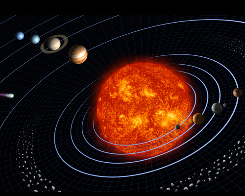
By the end of Lesson 11, you should be able to:
- Compare and contrast the interior structure and atmospheres of Mercury, Venus, Earth, and Mars;
- Qualitatively describe the process of tidal locking and relate this phenomenon to Mercury’s orbit around the Sun and the Moon’s orbit around the Earth;
- Describe the role impacts and collisions had on the evolution of the Inner Solar System planets and the Moon;
- Compare and contrast the terrestrial planets and the Jovian planets;
- Describe the processes for the formation and evolution of ring systems around giant planets;
- Compare and contrast the moons of the Jovian planets;
- Relate the appearance of the Jovian planets to atmospheric processes;
- Describe the relationship between Pluto and the Kuiper Belt;
- Explain the origin of comets and their distribution in the Solar System;
- Describe the process by which a “shooting star” appears in the night sky.
What is due for Lesson 11?
Lesson 11 will take us two weeks to complete.
Please refer to the Calendar in Canvas for specific time frames and due dates.
There are a number of required activities in this lesson. The chart below provides an overview of those activities that must be submitted for Lesson 11. For assignment details, refer to the lesson page noted.
| Requirement | Submitting your work |
|---|---|
| Lesson 11 Quiz | Your score on this quiz will count towards your overall quiz average. |
| Unit 4 Lab | During Lesson 11, you will work on, and complete, the Extrasolar Planets lab (Lab 4). |
Questions?
If you have any questions, please post them to the General Questions and Discussion forum (not email). I will check that discussion forum daily to respond. While you are there, feel free to post your own responses if you, too, are able to help out a classmate.
The Earth / Moon System
Additional reading from www.astronomynotes.com [43]
- Atmospheres [513]
- Planet Surfaces [514]
- Planet Interiors [515]
- Earth [516]
We are going to begin this lesson with a study of some of the properties of the Earth. We are going to focus on some of the physical processes that occur on Earth, and then we are going to discuss how the other inner planets differ from our observations of the Earth. We will emphasize the interior, the crust, and the atmosphere.
Atmosphere
The Earth has an atmosphere that consists of a mix of various gases (roughly 80% nitrogen and 20% oxygen, with small traces of argon, carbon dioxide, water vapor, and others) that is retained by the Earth's gravity. The Moon has no atmosphere today because its gravitational field is weaker than Earth's, and it wasn't strong enough to retain whatever primordial gases were there originally. The atmosphere helps to regulate the temperature on the Earth, keeping it within a fairly narrow range from day to night. On the Moon, the temperature can vary by 300 degrees during one Moon day — it is hotter than boiling water when the Sun is directly overhead on the Moon and is much colder than water's freezing point on the night side of the Moon.
The temperature on Earth is influenced by the Greenhouse Effect (this name comes from an analogy that isn't perfect, but is close enough for our purposes). This works as follows:
- The Earth absorbs visible light from the Sun.
- The Earth's surface heats up and radiates light in the infrared part of the spectrum.
- Water vapor and carbon dioxide (primarily) in the atmosphere absorb the infrared light from the surface, heating up the atmosphere.
- The atmosphere radiates infrared radiation at the surface of the Earth, also heating it up.
When this process is in equilibrium, the temperature of the Earth varies around a mean temperature from year to year. The discussion about global warming arises from the observation that the increase in carbon dioxide in the atmosphere (mostly due to humans burning fossil fuels) correlates with the steady increase in the mean temperature of the Earth because of an increase in the magnitude of the greenhouse effect.
Apart from the fact that we breathe the gas in the Earth's atmosphere and that the atmosphere keeps the temperature of the Earth warm enough for us to exist, the atmosphere also has played a role in shaping the Earth's surface. We do not see very many craters on the Earth, although there are a few, including "Meteor Crater," or "Barringer Crater," in Arizona.

On the Earth, the atmosphere protects us from the impacts of some objects, but the weather also erodes craters over time, making them no longer visible. Satellite images reveal the existence of some ancient craters on Earth, including Manicouagan Crater.

Try this!
Using the free application "Google Earth [519]," you can tour the Meteor Crater and Manicouagan Crater from Google Earth to get a sense of their real scale. Can you find any other craters on Earth using Google Earth? If you want to skip right to the answer, you can see the database of currently identified craters in the "Earth Impact Database [520]".
You can compare the Google Earth images of the surface of the Earth to the Google Moon [521] images of the surface of the Moon (Note: In the Google Earth application, you can now also bring up the 3D map of the Moon; instructions are available on the Google Moon website). How does the appearance of the Moon's surface differ from Earth's?
The Moon is very different. Since it lacks an atmosphere, most of the impact craters that formed on its surface are still visible today, and they will never erode away like those on Earth.
Crust and Interior
When we discuss the surface and the structure of the planets, we are going to focus on their density, because this property tells us a lot about the composition of the planet. Recall, the density is the mass of an object divided by its volume. If you consider comparing a cube of sugar to a cube of lead that is the same size, you will expect the cube of lead to feel heavier than the cube of sugar. This is because in the same volume (a cube of the same size), the lead will contain more mass than the sugar. The metric system was designed so that one cubic centimeter of water has a mass of 1 gram, so we say that the density of water is 1 gram per cubic centimeter (or equivalently, 1000 kilograms per cubic meter, which is another popular unit of measurement for density). The rocks and metals that we are familiar with are all denser than water. A typical rock has a density of about 3 g / cm3 and a typical metal (say iron) has a density of about 8 g / cm3.
Our measurements of the Earth's mass (from Kepler's Laws) and its volume (from its measured size) tell us that its average density is about 5.5g / cm3 — about half way between rock and iron. By studying data from earthquakes around the world, geologists have determined that the Earth is not uniformly made up of the same material. Instead it is differentiated into different layers. We live on the crust. Below the crust is the mantle, and below the mantle is a core. The crust is about 3 g / cm3 and the inner core is about 12 g / cm3, which suggest the crust is made up mostly of ordinary rock, and the inner core is denser than the metal lead. The mantle is a rocky layer intermediate in density between the crust and the core, and it is semi-fluid, somewhat like the consistency of bubble gum or flexible plastic. The crust of the Earth sits on top of the mantle, and because of convection (a process which occurs in fluids with a temperature difference between different layers — the warmer fluid rises, cools off, and then sinks, creating a flow) in the mantle, the plates that make up the crust are very slowly moving with respect to each other. This process of plate tectonics is the cause of earthquakes, the source of mountains and trenches under the oceans, and is one you will discuss in much more detail in the other courses in this program (e.g., EARTH 501 and EARTH 520). For the purposes of ASTRO 801, you should keep in mind though, that on Earth, plate tectonics is ongoing. We will want to consider if this is true of the other objects in the Solar System as we compare and contrast the planets and moons.
The Moon is very different. The average density is 3.3 g / cm3, but more importantly, there is less variation in the density from core to crust than the Earth. The Moon is not geologically active — there are no volcanoes or plate tectonics on the Moon. Equipment left behind by the astronauts who landed on the Moon has detected Moonquakes, but they are very mild. Interestingly, it looks like the core in the Moon is off center. The crust is about 60 km thick on the near side (facing Earth), but it is 150 km thick on the far side. In 2014, my Penn State colleagues published a new study [522] suggesting that this variation in the thickness of the Moon's crust was caused by the very hot, molten Earth heating the Earth-facing side while the far side of the Moon cooled off.
The surface of the Moon shows two very different regions. The dark regions (the Maria) are lowlands that were filled in by molten mantle material (lava) about 3.5 billion years ago. The light colored areas are highlands that are made of the original crust of the Moon. You can tell that the Maria are younger than the light colored regions because they have fewer craters. Originally, there were just as many craters in the Maria region as there are everywhere else, but when the molten rock filled in these regions and solidified, it covered many of them. Because the Moon has no atmosphere, the craters are very well preserved, giving us details on what the number of impacts was like in the early history of the Solar System. In the image below, you can see the Maria have few craters, while the other regions of the Moon are speckled with dark craters.

The far side of the Moon (the half that is never pointed towards Earth) looks very different from the side that we see; there are no Maria. This is attributed to the difference in the crust thickness. Since the far side of the Moon is about twice as thick, Lava was not able to penetrate the crust to fill in the lowlands, solidify, and create Maria.

The current leading theory for the formation of the Moon suggests that it was created in a collision between the proto-Earth and a Mars-sized object. Computer simulations of a collision like this show that the material that breaks off of the proto-Earth should wind up coalescing into a Moon-sized object in orbit around the Earth. The material that created the Moon would have come from the crust and mantle of the proto-Earth, which explains its lower density than the Earth. There is an excellent visualization of this in the video "Cosmic Collisions", which was released by NASA and the American Museum of Natural History. AMNH appears to have removed all of the public links to the video, but the History Channel has a good, similar video [527] that includes most of the details in the Cosmic Collisions video.
Tides
Additional reading from www.astronomynotes.com [43]
- Tides [528]
The Earth and the Moon directly influence each other, so it is best to think of these two objects as part of one larger system, rather than two separate, individual objects. Compared to the Earth, the Moon is relatively large. It has 1% of Earth's mass, and has 1/4 the Earth's radius. The Earth and Moon can almost be considered a binary planet system. The most notable influence that the two objects have on each other is tides.
The figure below shows the force of gravity felt by the Earth from the Moon. It is strongest just below the Moon and weakest on the side of the Earth opposite from the Moon (as indicated by the arrows). After you subtract off the mean force, you are left with the schematic diagram of the Moon's differential gravity field on the Earth in the bottom of the image. This shows how the Moon tidally deforms the Earth, creating two areas of high tide per day. This effect is most noticeable as the oceans and other bodies of water respond to the Moon's gravitational tidal force. Below the Moon, ocean water, for example, gets pulled into a high tide. One way to think of the reason for the high tide on the opposite side of the Earth from the Moon, is that the water gets "left behind", because it isn't being pulled as strongly as the center of the Earth, so there is a high tide on that side, as well. On the two sides of Earth perpendicular to the Moon, the net effect is that the water gets squeezed towards the center of the Earth, causing low tides at these two locations. As the Earth rotates once around during a 24 hour day, each location goes through high tide, low tide, high tide, and low tide.

For an animation of this effect as the Moon orbits the Earth, see NOAA's animation of the tides [531], which is part of a detailed tutorial on the tides [532].
In the animation on the NOAA site, you can see how the Sun also contributes to the tides on Earth. The tidal force on the Earth from the Sun is weaker than the tidal force on the Earth from the Moon. The way we observe the effect of the Sun is that when the Moon is in its Full or New phase, the Sun enhances the tidal effect of the Moon, leading to higher high tides. These are called spring tides. When the Moon is at 1st or 3rd Quarter (i.e., the Sun/Earth line is perpendicular to the Moon/Earth line), the Sun's tidal force cancels some of the Moon's tidal force, leading to lower than normal high tides. These are called neap tides. The images below illustrate the difference between the two.

Check it out!
You should note that even though many images in textbooks and from reputable sources like NOAA show the tidal bulge of the Earth pointing directly at the Moon, the true behavior is that the bulge is not aligned perfectly with the Moon—there is a delay.
Tides in the Earth/Moon system have led to an effect called tidal locking, and the Moon is now in a synchronous orbit (its rotation period is equal to its orbital period around the Earth). This effect is common, and occurs in many other systems. In the case of the Earth/Moon, this is how it works:
- The tidal bulge on the Earth rotates as the Earth rotates, and in general, the high tide bulge doesn't point straight at the Moon like in the image above. Instead, as illustrated in the ClassAction animation, the Moon lags behind the bulge.
- The force of gravity from the Moon pulls the deformed Earth in the direction opposite to its rotation, causing the Earth's rotation period to slow down. You might remember this by thinking that the tidal bulge is shifting in order to line up with the object causing it.
- The Moon gets deformed by the Earth, too, although since there is no water on the Moon, the effect isn't as obvious. However, the tidal bulge on the Moon has already shifted so that it points directly at the Earth. This is why the Moon always points the same face to the Earth.
- Because of Newton's third law (equal/opposite reaction), as the Earth slows down because of the Moon's pull, the Earth is pushing the Moon slowly away from the Earth. It gets farther away from us year after year.
Summary
To summarize the Earth/Moon system, we find that the two are rocky objects with different densities. Both are differentiated, with different layers of different density material in the crust, mantle, and core. The Earth's crust changes over time (plate tectonics) and the Earth's atmosphere continues to evolve, too. The Moon's crust is mostly unchanged since the event that created the Maria, and its lack of atmosphere means that the surface is unlikely ever to change. The Earth and Moon directly influence each other through tides, and the Moon has actually achieved a tidal lock to the Earth, which causes it to keep one face permanently pointed at the Earth. We will find that the other planets in the inner Solar System share some of the properties of the Earth / Moon system, but each also has some of its own peculiarities.
We should expect that the phenomena and the processes that influenced the Earth and the Moon during their evolution should have also influenced the other planets, as well. For example, tidal locking is observed in other parts of the Solar System (and other solar systems and star systems), too.
The Inner or Terrestrial Planets
Additional reading from www.astronomynotes.com [43]
- Earth-Venus-Mars [534]
- Mars [535]
Start Here!
Please review the properties of the Inner Planets at Bill Arnett's Nine 8 Planets website [536], an excellent resource.
Additionally, there is a great deal of information (with no annoying ads, like in the previous link) at NASA's Solar System Exploration page [537].
Our goal for this lesson is to come up with a list of the similarities between the planets, some trends in their properties, and an understanding of where some of the discrepancies in their properties may lie. To achieve this, we can begin with a simple bullet list that includes a summary of the properties of each of the three Terrestrial planets:

Mercury
- Surface heavily cratered—in some ways very similar to Earth's Moon.
- Very dark—only reflects a small amount of Sunlight (it has a low albedo).
- Temperature on the surface varies from 100K to almost 700K.
- In a 3:2 synchronous orbit with the Sun—three Mercury days (59 Earth days each) = two Mercury years (88 Earth days each).
- The iron core of Mercury is very large, taking up most of the interior of the planet and creating a relatively strong magnetic field for a planet of its size.
- No moon.
- Less than the size of the Earth.
- Visited by satellite Mariner 10—most of our knowledge comes from this one mission. The NASA Messenger mission [538] studied Mercury in recent years; it entered orbit around Mercury in March 2011 and studied it continuously before crashing to the planet's surface in 2015.
- Messenger somewhat surprisingly revealed that Mercury has water ice in shadow in craters at its poles!

Venus
- Thick atmosphere and "runaway greenhouse effect" causes 730K surface temperatures.
- Atmosphere consists mostly of CO2 (carbon dioxide), clouds of sulfuric acid—no water vapor or oxygen.
- Huge volcanoes.
- Clouds are highly reflective (high albedo)—Venus is one of the brightest objects in our night sky.
- Rotates very slowly (243 Earth days) and it rotates in a retrograde manner (opposite of the Earth & Sun).
- Not in a synchronous orbit—one Venus year = 225 Earth days.
- No moon.
- Almost identical in size to the Earth.
- A number of missions to Venus have been sent by the USA and USSR. In 1994, Magellan mapped the surface of Venus.

Mars
- Temperature always below the freezing point of water.
- Giant volcanoes (largest of any in the entire Solar System).
- Intense, large-scale dust storms.
- Has an atmosphere that is much thinner than Earth or Venus, mostly CO2.
- The surface is red because of the presence of iron oxide (rust).
- One Mars day is only slightly longer than an Earth day (24.6 hours).
- One Mars year is 1.88 Earth years.
- Polar caps of dry ice and water ice that change with the seasons.
- Frozen water in a permafrost layer (recently confirmed).
- About half the size of Earth.
- Two small, irregularly shaped moons—Phobos and Deimos.
- The most visited planet in our Solar System, including several recent missions, Mars Exploration Rovers Spirit and Opportunity, the Phoenix Lander, Curiosity, and MAVEN.
Interior structure
There are several peculiarities about these planets, but we can understand the likely causes of these properties when we contrast them to the Earth. First, consider the interior structure of these planets. Just like the Earth, Mercury, Venus, and Mars are differentiated. Curiously, we find that, compared to the other planets, Mercury's core is relatively large. That is, it fills up most of the interior of this planet. Because the core of Mercury is probably mostly made up of iron and nickel and it fills so much of the planet's interior, Mercury is the densest inner planet. We expect that some of the core of each of the inner planets is molten, and we expect that this liquid metallic core must generate electric currents inside the planet as the core rotates with the rest of the planet. These electric currents should create magnetic fields, making the planets behave as if they have giant bar magnets inside them. Both Mercury and the Earth have measurable magnetic fields, but, contrary to our expectations, Venus and Mars do not. For Venus, the reason may be that it rotates too slowly to create the necessary conditions to create a magnetic field. The lack of magnetic field on Mars may be caused by its lack of a molten core.
Albedo
We observe the inner planets easily because they are nearby and shine by reflecting sunlight. You can see Mercury, Venus, and Mars at different times of the year without any instruments like a telescope or binoculars—all three of these planets are visible to your naked eye. Although all of the planets reflect sunlight, different materials reflect different amounts of sunlight. For example, look at the Earth at the NASA: The Blue Marble site [541]. We see that the brightest parts of the Earth are the clouds and the ice near the North Pole. The darkest parts of the globe are the patches of deep ocean that are not covered by clouds. The amount of light reflected by a surface is called the albedo. For light colored clouds, the albedo is high, and much of the incoming sunlight gets reflected. Water and dark colored rock reflect much less light. Mercury is mostly covered by dark rock, so its albedo is very low. On the other hand, Venus is covered by a thick layer of clouds, so it reflects almost all of the Sunlight that hits it. Because of Venus' high albedo and its proximity to the Earth, it is the brightest object in the night sky after the Sun and the Moon.
Atmosphere
Observations of these planets tell us that all three have atmospheres. Mercury has a very thin atmosphere with a strange composition. Mercury is so small that gas easily escapes from its gravitational pull, so its atmosphere must be regenerated continually, perhaps by the bombardment of the surface of the planet by energetic particles from the Sun. Venus, on the other hand, has a thick, dense atmosphere. The greenhouse effect has "run away" on Venus, making the surface temperature hotter than Mercury, even though it is farther from the Sun. Mars' atmosphere is much thinner than Venus or Earth, and it consists primarily of carbon dioxide. The atmosphere of every inner planet originated when the planet was formed and has been supplemented by gas that has escaped from underneath the crust.
The laws of physics tell us that the hotter a gas is, the faster the particles inside that gas move. For Mercury and Mars, these planets are so small that they have weak gravitational fields, which means that much of the gas in their atmosphere can escape if it is warm enough (the average speed of the particles in the gas exceeds the escape velocity from the planet). For Venus and the Earth, which are more massive and have stronger gravitational fields, the lightest gases can escape, but gases like carbon dioxide and nitrogen do not.
Additionally, on the Earth, we know that plant and animal life process the gas in the atmosphere. For example, humans breathe oxygen and exhale carbon dioxide, while plants use carbon dioxide and produce oxygen. Because of these biological processes on the Earth, our atmosphere has evolved significantly from its original content. The Earth's atmosphere may have once been much like Venus' atmosphere is now, however, as plant life on the Earth arose, the process of photosynthesis contributed to the removal of carbon dioxide and the increase in oxygen content.
Rates of rotation
There is also some diversity in the rotation rates of the inner planets. We are most familiar with the Earth. It rotates in a counterclockwise direction in close to 24 hours. Mars is quite similar to the Earth. Its rotation axis is tilted by 24 degrees (Earth's axial tilt is 23.5 degrees), and its rotation period is just over 24 hours. So on Mars, the length of the day and the variations in the height of the Sun above the horizon over the course of one Mars year are similar to what we are used to on the Earth. Mercury has become tidally locked to the Sun, similar to how the Moon is locked to the Earth. However, in the case of Mercury, the planet rotates in 59 days and orbits the Sun in 88 days. What this means is that Mercury rotates completely on its axis (that is, 360 degrees) 3 times in the same amount of time it takes to orbit the Sun 2 times. This is referred to as a 3:2 resonance. In the case of the Moon, since it orbits the Earth 1 time in the same amount of time as it rotates 1 time, this is referred to as a 1:1 resonance. Although this seems a bit peculiar, Venus' rotation properties are much stranger. It takes 243 days to rotate once (and there is no tidal locking, so the Venus year has nothing to do with the Venus day), but it rotates in the opposite sense compared to Mercury, Earth, and Mars. All of these planets orbit the Sun in a counterclockwise direction, and Mercury, Earth, and Mars rotate counterclockwise around their axes. Venus rotates slowly in a clockwise manner around its axis. One theory is that a collision or collisions with Venus by other objects caused its rotation sense to reverse, but an alternative theory is that the tidal influence of the Sun and the other planets in the Solar System may also have caused this unique rotation.
Want to learn more?
Recall that Starry Night allows you to travel to the surface of each planet. If you would like to compare the rotation rates, orientation of the axis of rotation, and orbital periods for each planet, you can travel to Mercury's, Venus', or Mars' surface, set the time flow rate to 3000x (or the time step rate to say 1 Earth day), and as time goes by note the location, date, and time of sunrise and sunset, the height of the Sun above the horizon, and the length of 1 day on that planet.
You can also choose to hover over a point on the surface, and if you choose to hover over the north pole of each planet, you can watch them rotate below you. For Venus, you will have to turn up the time flow rate to a very high number in order to see it rotate at all.
Jupiter
A course on astronomy requires you to try to understand much larger numbers and much larger units of measurement than we are used to in our day to day experience. For example, we have already studied the distances to stars, the sizes of galaxies, and the age of the observable universe, all of which are very large (tens of trillions of kilometers, millions of trillions of kilometers, billions of years). Now that we are studying the Solar System, the planets are tiny relative to stars, galaxies, and the universe.
With this in mind, though, if we compare the planets to each other, Jupiter is the largest, and it is an immense planet. In our everyday experience, Earth seems large, since it has a diameter of more than 12,000 kilometers. Jupiter is about 12 times larger in radius, which means that it is about 1400 times larger in volume than the Earth (that is, about 1400 Earths could fit inside Jupiter).
If Jupiter was made of similar materials as Earth (iron core, rocky crust), then its mass would be about 1400 times larger than Earth, too. However, we find that Jupiter's mass is only 300 times larger than Earth, which tells us that its density (its mass divided by its volume) must be smaller than Earth's. Here is how you can convince yourself this is true:
If you recall our discussion of density previously, water has a density of exactly . Does this mean that Jupiter is made of water, and if so, what form is it in (water vapor, ice, liquid water)?
In fact, Jupiter is not made of water. Its composition is very similar to the Sun's. It is made up primarily of Hydrogen and Helium, with traces of other elements and molecules. Observations of Jupiter show us that what we see as its “surface” is in fact its atmosphere—the observable portion of this planet is entirely gaseous. Look at the following image from the Cassini satellite.

If you look at some of the fine details in the image, you will not see anything that looks like the continents on Earth, the craters on Mercury, or the rocky plains of Mars. Instead, it looks more like the clouds of Venus, which obscure that planet's surface. Animations, such as the Cassini movie of the Great Red Spot [543] produced from images taken by the Cassini satellite, show that the visible atmosphere is in constant motion, and even appears to have nearly circular storms that do not look all that different from hurricanes on Earth.
The atmosphere of Jupiter shows a lot of structure. It has alternating dark and light colored bands, which are not smooth, but which contain swirls and eddies. One of the reasons for the banded structure in Jupiter's appearance is that convection is occurring in the atmosphere. Convection occurs when you have a temperature difference between the layers in a liquid or gas. The common example is putting cream in a cup of coffee—since the cream is colder than the coffee, it sinks to the bottom, where it heats up. Then, when it heats up, it rises to the top, where it cools off, and then sinks again. So the process of convection creates a circular current in the fluid. This is going on in Jupiter's atmosphere, and what we observe as the different colored bands are actually different layers in the atmosphere. The light-colored areas (called zones) are the bands that are rising, while the dark-colored areas (called belts) are the layers that are sinking. As the “air” (the mix of gases that makes up Jupiter's atmosphere, which is different than air on Earth) rises, clouds form out of different materials—water, ammonium hydrosulfide, and ammonia. The whitish zones are the high layers of ammonia clouds, while the darker belts are the lower layers of ammonium hydrosulfide clouds. The exact cause of the colors remains an open question for researchers. Inside the clouds, reactions between sunlight, lightning, and different chemical compounds probably give rise to the variety of colors seen in Jupiter's atmosphere, but exactly what processes give rise to which colors has not been determined yet.
Jupiter has been visited by several missions, the most recent being Juno [544]. Juno passed very close to Jupiter, and, in particular, studied its polar regions. This mission revealed previously unknown details about Jupiter, like every NASA Solar System exploration does when it visits a world.
Just like in the atmosphere of Earth, storms develop in the atmosphere of Jupiter. Unlike the Earth's atmosphere, however, some of the very large storms achieve a level of stability that allows them to persist for hundreds of years, and perhaps even longer. The most famous storm in Jupiter's atmosphere is called the “Great Red Spot,” which is a rotating storm larger than the Earth! Here are some photos of this famous storm:
- APOD: The Great Red Spot [545]
- APOD: The Great Red Spot and the Smaller White Oval [546]
- Hubblesite: Changes in the Great Red Spot [547]
Smaller storms in Jupiter's atmosphere appear, disappear, merge, and change in relatively short time scales. However, the Great Red Spot has persisted for at least 300 years. It can be seen to change over time. The Great Red Spot has some similarities to hurricanes on Earth, with the main difference being hurricanes are clockwise rotating, low pressure storms, while the Great Red Spot is a counterclockwise rotating, high pressure storm. On Earth, when these storms hit land, they can lose energy quickly, and the storm will dissipate. Since the Great Red Spot has not dissipated, this tells us that (1) there is some source of energy continually supplying it with enough to remain stable, and/or (2) there is no solid land underneath it to cause it to lose energy rapidly.
Although astronomers have no direct way of observing Jupiter's interior, we have some evidence that suggests what it may be like. Although this planet is made up primarily of hydrogen and helium, which are found in gas form on Earth in normal conditions, the conditions in Jupiter's interior are unlike those on Earth. Given the temperature and pressure on Jupiter, we think that most of the planet is actually liquid hydrogen. What lies beneath this liquid layer is even more of a mystery. We expect that there may be a small solid core (about the size of the Earth) at the very center of Jupiter that is made up of rock, metals, and solid compounds of hydrogen.
If you recall our discussions of the night sky, we discussed how many of the planets are easily visible to the naked eye. The inner planets do not emit any of their own light. Instead, they are visible because they reflect sunlight. This is not strictly true for Jupiter. If you measure how much total light it emits, it is more than the amount of sunlight that reaches the planet. Like the persistence of the Great Red Spot, which suggests some internal mechanism is providing energy to the cloud layers, the fact that Jupiter is giving off more light than it receives also suggests there is some internal energy generation. When we discussed protostars, we saw how they generated energy through gravitational contraction before nuclear fusion began. In the case of Jupiter, it does not contain enough mass to ever achieve the internal temperature and pressure to begin nuclear fusion, but it can generate energy through gravitational contraction.
The Outer or Jovian Planets
Additional reading from www.astronomynotes.com [43]
- Rings [548]
Through even a small telescope, both Jupiter and Saturn look beautiful. Many people, myself included, feel that Saturn is by far the most beautiful of all of the planets. Much of Saturn's aesthetic appeal comes from its magnificent ring system.

The rings of Saturn orbit the planet around its equator, and, although they are very thin, they extend out almost 300,000 kilometers from the planet. The pair of images from Hubblesite shown below will help you understand exactly how thin they are—when we see them nearly edge-on, they almost disappear!

Even though they are 300,000 kilometers in radius, Saturn's rings are only about 20 meters thick. An analogy is to picture a compact disc (CD) that is the same thickness as usual, but 30 kilometers (about the size of an average town) in diameter!
The rings of Saturn were probably created by the destruction of an object that got too close to the planet. We know that Saturn's rings are made up of many small particles. Even though they look like they may be solid in all of the images that you have seen, they are not! If you look back at our discussion of tides in the last lesson, we studied how the gravitational force of the Moon deforms the Earth and vice versa. If you think about it, if a tidal force is strong enough, it might be able not only to deform an object, but also to actually break the object into pieces. There is a limit, called the Roche limit, which is a roughly spherical region that surrounds each planet (and star). Outside the Roche limit, an object will be deformed by the planet's tidal force, but will otherwise be OK. If an object gets inside the Roche limit, though, the tidal force from the planet will be stronger than the force of gravity holding the object together, so it will be destroyed. The rings of Saturn are inside of the Roche Limit for this planet, so it seems likely that they were formed by the disruption of some massive object.
From the ground, there only appear to be a few rings with a relatively wide, dark gap called the Cassini Division between the rings. However, views from spacecraft like Voyager and Cassini show that the rings are actually made up of many thin ringlets. It appears that there may be up to several hundred thousand ringlets.

Other than its ring system, however, Saturn is in many ways similar to Jupiter. It is the second most massive and second largest planet in the Solar System. Saturn rotates once on its axis very quickly, about 11 hours, which is very similar to Jupiter, which rotates in approximately 10 hours. If you look at an image of the whole disk of Saturn, you find that it appears to be not quite spherical, but it is flattened because of its fast rotation. Saturn is, again, primarily a gaseous planet with perhaps a small solid core, but its density is significantly different from Jupiter's—it is 0.7 g / cm3, which is less than water! An often repeated joke is that if you could build a bathtub big enough, Saturn would float, but it would leave a ring.
In most pictures, Saturn's atmosphere appears to have less structure than Jupiter's. This is very likely because the colder temperature of Saturn causes different chemical reactions to occur in the atmosphere. However, if you process the images to enhance the contrast, you will see that the atmosphere of Saturn does show many of the same structures that we see on Jupiter, as shown in these Hubblesite images:
Uranus and Neptune
Every planet that we have studied so far was known to ancient astronomers because they are all visible to the unaided eye. Uranus and Neptune, however, are only visible with a telescope. In many ways, these two planets seem similar, but when we study them in some detail, we will find that they have some significant differences. Both Uranus and Neptune are gaseous planets like Jupiter and Saturn, but they are much smaller. They are both about 4 times the diameter of the Earth, and they are about 15 times more massive than Earth. Although this is large, for perspective it is 20 times less massive than Jupiter.

Images of these two planets show that in natural color, Uranus and Neptune look to be a blue-green color. This is usually attributed to the presence of a mix of methane and molecular hydrogen in the atmospheres of these planets. The atmosphere of Uranus appears to be very plain. It does not show banding, storms, or any of the features seen on Jupiter or Saturn. However, the Voyager satellite did show dark spots on Neptune that appear to be storms similar to the Great Red Spot on Jupiter.

It seems very strange that Neptune should show such strong evidence of activity in its atmosphere when Uranus does not. In the case of Uranus, it is very cold—only about 58 kelvin. It also does not show any evidence of generating energy in its interior, so it is believed that the lack of internal energy generation keeps the atmosphere from creating the prominent structures seen in Jupiter and Saturn. Neptune is even more distant than Uranus, so we expect that it should be colder. The measurement that Neptune is 59 kelvin (that is, slightly warmer than Uranus) suggests that it does generate energy, emitting almost 3 times as much light as it receives from the Sun. So, it may be that it requires internal energy generation to create the strong weather patterns in the gas giants. Why, then, is Uranus the only Jovian planet which does not appear to generate energy in its interior?
Recent observations by Hubble [556] shows that Uranus' atmosphere is beginning to show new structure. Uranus, it turns out, has a very strange rotation. Most of the planets rotate so that the poles of their rotation are pretty closely aligned with the poles of their orbit. Another way to visualize this is that the equator of most planets is aligned with the plane of the planet's orbit around the Sun. However, the pole of the rotation of Uranus is almost perpendicular to its orbit. That is, the pole of Uranus' rotation is tilted by almost 90 degrees compared to that of Earth. Because of this, Uranus keeps its pole pointed towards the Sun and not its equator. So for about 1/4 of its orbit, its South Pole never sees the Sun, and for 1/4 of its orbit, its North Pole doesn't see the Sun. It takes Uranus 84 years to orbit the Sun once, and just a few years ago its South Pole started getting sunlight again. This may be why its atmosphere is beginning to increase its activity compared to when Voyager visited decades ago. Thus, it may be that Uranus' odd rotation may be responsible for its apparent difference from the other Jovian planets in terms of its internal energy generation.
There is one other peculiar feature of Uranus, but this one it shares with Neptune. The gas giant planets have magnetic fields, just like Earth. In fact, Jupiter has an incredibly intense magnetic field. Uranus and Neptune both have magnetic fields, but in each case, the center of the field is offset from the center of the planet, and the pole of the magnetic field is significantly offset from the pole of the planet's rotation. In the case of the magnetic fields on Earth and Mercury, we think that these are created by a rotating liquid metallic core. The proposed model for the magnetic fields in Uranus and Neptune is that in their case they are created in an outer layer and not in the core, which can lead to their measured offsets from the core and the rotation axis of the planet.
Rings and Jovian Moons
Additional reading from www.astronomynotes.com [43]
- Jupiter's Large Moons [557]
- Titan, Enceladus, and Triton [558]
Ring systems
Saturn is the only gas giant planet that has a prominent, easily observable ring system. However, observations have revealed that each of the Jovian planets have ring systems. Jupiter's ring is exceptionally faint. The particles in Jupiter's ring are smaller than those in Saturn's rings and do not reflect light as well.

Uranus also has rings, and the images that reveal its rings emphasize how tilted this planet is compared to Saturn. The images show that the rings appear vertical, while those in Saturn are horizontal. Like Jupiter, the particles in the rings of Uranus are smaller than those in Saturn's rings. They also do not reflect light well. In the case of Jupiter and Uranus, our physical models suggest that the particles should not be able to remain in the rings very long, thus the rings should dissolve over time. Therefore, we suspect that the ring systems of the giant planets may be relatively young—only a few hundred million years old—compared to the nearly 5 billion-year-old age of the planets themselves.

Neptune also has a ring system, but it is not as well observed as those of the other planets. It appears to also contain dust grain-sized particles, but one peculiarity is that its rings are more "clumpy" than those of the other gas giant planets.

Jupiter's moons
Each of the gas giant planets can be thought of as its own mini version of the Solar System. Each planet has a large system of moons which are in orbit around it. Jupiter has more than 60 moons, Saturn has more than 30, Uranus more than 20, and Neptune more than 10.
Exactly how many moons does each Jovian planet have?
When asked this question, I do not often quote a firm number of moons, because astronomers continue to find more. Instead, I usually simply say, for example, that Jupiter has more than 60 moons.
An example of a moon discovered recently (although it is associated with Saturn, not Jupiter) is found in a press release from the NASA Cassini mission [562]. Much more recently, some of Jupiter's "lost" moons were found again, and two new ones were discovered [563]. Jupiter is now inching closer to 70 moons.
The four biggest moons of Jupiter are famous in the field of astronomy because they were part of the revolution to a heliocentric understanding of the Solar System. If you recall back in the earliest lessons in this course, we studied that the ancient astronomers believed that the Earth was the center of the Universe and that all objects (the Sun, the planets, the stars) orbit the Earth. When Jupiter was first observed through a telescope by Galileo, he discovered four moons orbiting this planet, which was evidence that not every object orbited the Earth. This important observation was very influential in the debate over the heliocentric vs. geocentric models of the Solar System.
In modern times, we have observed these four moons in detail, because they are by far the largest of Jupiter's moons and each one has its own interesting properties. They are classified as moons because they orbit Jupiter, but these objects are so large that if they were to orbit the Sun on their own, they might be called planets. The four Galilean moons of Jupiter are called Io, Europa, Ganymede, and Callisto. Their properties are briefly described below, followed by links to images highlighting specific features of those moons.

- Io: The innermost of Jupiter's Galilean Moons is very active. Because of the constant deforming of the surface of this Moon by Jupiter's tidal force, the interior of Io is continuously heated, which leads to many active volcanoes on its surface. The moon has over 100 volcanoes that erupt frequently and constantly alter the surface of this moon. Io, therefore, has the youngest surface of any solar system object.
- APOD: Io's surface [565]
- APOD: Active volcano on Io [566]
- Europa: Each of the Galilean moons is different in appearance. Europa and Io look nothing alike. The surface of Io looks bright yellow from the sulfur and sulfur compounds emitted by its volcanoes. On the other hand, Europa looks to have a light colored, smooth surface with a network of darker stripes. The evidence from the Galileo satellite suggests that Europa's surface is mostly ice, which is sitting on top of a liquid water ocean. The dark stripes are probably caused by the ice cracking and refreezing. In fact, high definition images of Europa's surface appear similar to antarctic ice images taken from Earth-orbiting satellites. Because of the suspected presence of an ocean on Europa, scientists believe that there is a reasonable probability that life may exist on this moon, underneath the icy surface.
- Ganymede: This moon is the largest moon in the entire Solar System. It is bigger than the planet Mercury. Ganymede again has a different appearance than either Io or Europa. It has some smooth, dark regions with craters visible, and it also has some lighter regions that have deep grooves visible. Some of the surface features on Ganymede may be similar to the fractured ice features on Europa, but others appear similar to fault lines on Earth. Another unique feature of Ganymede is that this moon has its own magnetic field. Some astronomers argue that the magnetic field may be associated with a subsurface ocean on this moon, as well.
- Callisto: The surface of Callisto looks to be the most similar to our own Moon—it appears mostly dark and heavily cratered. The heavy amount of cratering tells us that the surface of this moon must be the oldest among the Galilean moons. There is a large crater with a diameter of several thousand kilometers on Callisto that was created by a major impact. It is somewhat surprising that Callisto survived this impact. Like Europa and Ganymede, recent observations from the Galileo satellite suggest that this moon may also have a subsurface ocean.
Other than the four Galilean moons, most of the rest of Jupiter's moons are small, irregularly shaped bodies that are most likely a mix of rock and ice. Jupiter is such a large planet that it has a strong gravitational pull. Thus, if a small object orbiting the Sun happens to pass too close to Jupiter, it can become captured into an orbit around Jupiter. It is very likely that many of the small moons of Jupiter are captured objects.
Want to learn more?
A comprehensive summary of the moons of Jupiter (and the other gas giants) is online at The Jupiter Satellite Page [574].
Saturn's moons
Like Jupiter, Saturn has several very large moons and then a few dozen small, irregularly shaped moons. The most famous of Saturn's moons is Titan, which has been known for several decades to have its own atmosphere. Titan, like Ganymede, is larger than the planet Mercury. For a long time, its surface was completely unknown to us. Its atmosphere is somewhat similar to smog on Earth, making it extremely difficult for telescopes to detect anything other than a uniform haze. See the image below, for example.

The chemical composition of Titan's atmosphere and its temperature and pressure have led astronomers to propose that there may be bodies of liquid methane and/or ethane the size of lakes on the surface and it may rain liquids that are similar to gasoline. Hubble Space Telescope images and images from the Cassini satellite mission to Saturn have finally allowed astronomers to penetrate the hazy atmosphere of Titan, revealing that it has surface features, including some that appear to indicate the presence of liquids. The Cassini satellite brought with it a lander that was sent through Titan's atmosphere and landed on its surface in early 2005. The images returned from the Huygens lander showed that much of the speculation about Titan's surface appears to be correct. It has features similar to rivers and lakes that appear to have contained liquid methane at some point. The material the lander landed on is similar in consistency to mud. The below false-color image from radar mapping of Titan's surface shows features that are proposed to be lakes of liquid on Titan's surface.

Want to learn more?
Cassini has completed surveying many of Saturn's moons, and, like the Galileo satellite mission to Jupiter, its results have revolutionized our understanding of Saturn's moons. We now have many impressive images of the larger moons of Saturn.
- APOD: Cassini's view of Enceladus [577] -- more recent analyses of Enceladus have discovered giant plumes of water and ice erupting from this Moon, which has led to studies suggesting that it, too, has a subsurface ocean.
- APOD: Cassini's view of Rhea [578]
- APOD: Cassini's view of Iapetus [579]
- APOD: Cassini's view of Dione [580]
- APOD: Cassini's view of Tethys [581]
Saturn does have many small, irregular moons, as well. In the Saturnian system, however, it seems like these moons play an interesting role with regards to the ring system. The gravitational pull of the moons can help keep the rings in narrow, tight orbits (any particle that strays from the ringlet will get ejected or pushed back into the ringlet by the force of gravity from a moon), or they can even clean out gaps in the rings. Here is an image of the moon Prometheus appearing to directly interact with the material in one of Saturn's rings.

The moons of Uranus and Neptune
The moons of Uranus and Neptune include several that have interesting surface features and properties like several of the larger moons of Jupiter and Saturn. No satellite mission since the Voyager 2 mission has visited these moons, though, so their properties are not as well studied yet as the Galilean satellites and Titan. Below is an image of Triton, a strange moon orbiting Neptune.

Overall, the moons of the Jovian planets are a diverse collection of objects that exhibit a wide set of properties. Many of the moons have been studied in detail by the recent Galileo and Cassini missions, but there is still much more for us to learn.
Pluto and the Kuiper Belt
Additional reading from www.astronomynotes.com [43]
We know that the Sun contains the vast majority of the mass in the Solar System. When we studied Kepler's Laws, we found that we can calculate the orbit of the planets just by figuring out how much the gravitational force of the Sun pulls on each planet. It turns out that this is mostly true. In reality, the gravitational pull of every planet does make minor perturbations on the orbits of the other planets. For example, Jupiter slightly alters the Earth's orbit (and vice versa), Saturn slightly alters Neptune's orbit (and vice versa), and so on. After the discovery of Uranus, astronomers noticed that its orbit was being perturbed by a larger amount than could be accounted for by the other planets known at that time. Thus, they predicted that another massive planet must exist beyond Uranus. Neptune was discovered based on these predictions. Even after this discovery, though, astronomers felt that perturbations in the orbits of Uranus and Neptune meant that another planet must still exist beyond Neptune.
Based on these predictions, Clyde Tombaugh carefully studied photographs of the sky and found a faint object that was moving compared to the background stars. The object discovered was not massive enough to perturb the orbit of Neptune, so its discovery appears to have been accidental! This object was named Pluto and was determined to be the ninth planet in the Solar System. However, as we have learned more and more about Pluto since its discovery, it appears to be different from our expectations in a number of ways.
Want to read more?
The story of the discovery of Pluto and the controversy over its current status is summarized very well in the book, Is Pluto a Planet? [585]
Another excellent book that discusses the discoveries of other, massive objects in the same part of the Solar System is How I Killed Pluto and Why it Had it Coming [586]. This is my personal favorite astronomy book, and I recommend it highly.
First of all, you should realize that Pluto is, by far, the most difficult of the nine historical planets to study. It is very distant and very faint, and so, prior to July 2015, no satellite had visited Pluto. The NASA New Horizons mission [587] performed a flyby of the Pluto system in mid-2015. The Hubble Space Telescope is not powerful enough to reveal much about the planet Pluto. Compare these Hubble Space Telescope images of Mars (top image) and Pluto (bottom two images) to see the difference in the quality of data on the two planets.


Now that New Horizons has provided us with much higher resolution images of Pluto and Charon, it is clear how fascinating these worlds are. The scientific work in analyzing these images is not yet done as of your time working on this course, however, many surprises have already been discussed by the New Horizons team. In particular, Pluto's surface appears to be much more active than was expected.
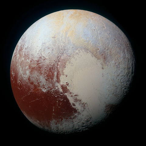
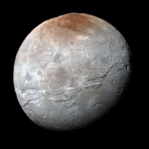
Prior to New Horizons study of Pluto, we discovered from the ground that Pluto has one large moon, called Charon (pictured above), which is roughly half the size of Pluto. Pluto is approximately 2300 kilometers in diameter and Charon is approximately 1300 kilometers in diameter. By observing the two objects orbit each other, we can also calculate their masses using Kepler's laws. We find that Pluto contains less than 1% of the mass of the Earth, and Charon is about 10% of Pluto's mass. Combining our knowledge of the mass of these two objects and their sizes, we can calculate their density, which comes out to approximately 2 g / cm3 and suggests that these objects are a mix of ices and rock.
The orbital properties of Pluto and its largest moon are also peculiar. Like Uranus, Pluto appears to have its rotational axis almost perpendicular to its orbital axis. That is, it is orbiting on its side compared to most of the planets in our Solar System. Charon's orbit around Pluto is aligned with Pluto's rotation axis, so, from our point of view on Earth, Charon appears to orbit Pluto perpendicularly to the path Pluto takes around the Sun. Perhaps the most peculiar aspect of Pluto's orbit is its inclination compared to the Earth's orbit around the Sun. If you define a plane containing the Sun and the Earth, you can measure the angle that each other planet's orbital plane makes with the Earth's orbital plane. Most of the other planets have orbital inclinations of less than 3.5 degrees from the Earth's orbital plane. Mercury is inclined by more than 7 degrees, but Pluto's orbit is inclined by almost 20 degrees. So, compared to the planets, Pluto's path takes it from a point high above the Earth's orbital plane to another point below the Earth's orbital plane. See the below image captured from Starry Night.

In recent years, there has been some controversy over the classification of Pluto as a planet. It is much smaller than the outer planets, and in fact, it is smaller than many moons, including Io, Europa, Ganymede, Callisto, Titan, and Triton. Its peculiar orbit also suggests that it may have had a different origin than the planets. Some astronomers suggest that perhaps Pluto is not a planet after all, but a different class of object. Recent discoveries of other, similar objects suggest that Pluto may be just one of a family of objects outside the orbit of Neptune.
Beyond Neptune, astronomers have discovered a large population of objects with sizes of about 100 kilometers or so up to more than 2000 kilometers [592]. These are called “Kuiper Belt Objects” or KBOs, after the astronomer Gerard Kuiper. There is some controversy about whether or not Kuiper predicted the existence of the objects that are named after him, so sometimes the class of objects are more simply referred to as trans-Neptunian objects or TNOs.
The Kuiper Belt is a region of space in the Solar System that is donut-shaped. Its inner radius is just past the orbit of Neptune at 30 AU, and it extends out to perhaps 50 AU or farther. The thickness of the Kuiper Belt is approximately 10 AU. Inside of this region perhaps up to 100,000 KBOs orbit the Sun!
Recently, several large objects have been discovered in the Kuiper Belt that has sizes similar to Pluto's moon, Charon. Some have formal, approved names, and others have informal names. The largest of these objects include: Quaoar, Haumea, Makemake, Orcus, Ixion and Varuna. There is an excellent, well-maintained image of these objects [593] to scale at Wikimedia Commons. To get a general idea of the properties of this class of objects, you can investigate further Quaoar as an example.
Want to learn more?
- The discoverer of the first KBO and many other KBOs maintains an in-depth website devoted to these objects, and it contains far more detailed information than I can include here. If you are interested, please visit The Kuiper Belt Page. [594]
- To investigate Quaoar, check out:
- The Discovery of Quaoar [595]
- Hubblesite: Quaoar [596]
- APOD: Quaoar [597]
The discovery of these objects in the Kuiper Belt with sizes comparable to Charon suggests that there are more large KBOs left to be discovered. Because these objects are small and extremely distant, they are difficult to observe. The brightness of many of them is comparable to some of the faintest stars in the Milky Way and to some of the faint galaxies in the Hubble Deep Field. Although several groups of astronomers have searched the sky for KBOs and found many of them, they expect that perhaps a few dozen more 1000 kilometer size KBOs remain undiscovered. There may even be several Pluto-sized KBOs, too. In 2016, it was suggested that there may be a planet similar to Uranus and Neptune in the Kuiper Belt based on evidence from the motion of several unusual KBOs. This object is being referred to as "Planet 9 [598]" by the researchers who proposed its presence, but it has yet to be found if it does in fact exist.
In 2003, an image taken by the team that discovered many of the other large KBOs included an object that was provisionally named 2003 UB313. Initial estimates revealed that it was perhaps larger than Pluto. For this reason, its discoverers and many in the community were expecting it to be named the tenth planet. The International Astronomical Union (the IAU) is the organization that approves the names of newly discovered objects in the Solar System. In 2006, they took on the task of defining the word planet. Instead of adopting a definition that would classify 2003 UB313 as a planet, they created a category of objects called dwarf planets. A side effect of this decision is that Pluto no longer fits the definition of a planet, but is classified as a dwarf planet too. After this decision, 2003 UB313 was given its official name of Eris, and we now know that it is more massive than Pluto, although the objects have been found to be quite closely matched in diameter.
While the new definition of a planet is firmly grounded in science, the names of classes of objects is really an issue of semantics. The point I impress when I'm teaching about the Solar System is that Pluto is still as large and as massive as it was when it was discovered. It follows the same orbit, and all in all, it is identical to the object it was before it was demoted from planet status. I think the terminology of dwarf planet is unnecessary. Instead, I prefer to point out that Pluto was the first large KBO discovered, and rather than being an oddball of a planet, it is the prototype of the class of large KBOs. I like to flip this particular question around with my undergraduate students. In classes where I have time and the resources, I ask students in groups to research and study the properties of all of the large, round objects in the Solar System. Then, I ask them as a group to answer the question, "How can we organize the large, round objects in the Solar System by their properties?". Planetary scientist and writer Emily Lakdawalla maintains an excellent image of all of the round objects in the Solar System less than 10,000 km in diameter [599], which can be used as a resource for students pursuing this investigation. If you study the properties, you do find that the terrestrial planets (Mercury, Venus, Earth, and Mars) have very similar properties and the Jovian planets (Jupiter, Saturn, Uranus, and Neptune) share properties. However, the other objects in the Solar System can be grouped in various ways, and Pluto shares properties with many other objects, but not with the planets. Often this leads to a discussion that the names we have traditionally used -- planet & moon -- are insufficient for categorizing these objects. It really does seem like we need to either call many dozens of objects planets, or only 8. There is no clean, scientific categorization of the large, round objects in the Solar System that leads to 9 planets with Pluto being the 9th.
Pluto has a larger albedo than most KBOs, making it appear brighter on Earth and easier to observe than most KBOs. However, in all other respects, Pluto is probably very similar to Eris, Quaoar, Ixion, and Varuna. So, while we now only recognize 8 planets, we have a number of new interesting objects to study in addition to Pluto. We continue to learn more about these objects. Eris is now known to have a small moon named Dysnomia, and Pluto was found to have two more moons, Nix and Hydra, in 2006, and two other new moons, Styx and Kerberos, in 2011 and 2012. [600] These were also imaged by New Horizons [601], but in far less detail than Pluto and Charon.

The story of the status of Pluto is likely to change, and I expect astronomers to continue to identify large KBOs. The story to date has been exciting, and I recommend investigating it much more deeply than we have here.
Want to learn more?
- The IAU has an informational website [603] on their role in the debate over the status of Pluto.
- Mike Brown maintains a highly detailed website [604] on the discovery of Eris and his feelings about its classification.
Comets
Additional reading from www.astronomynotes.com [43]
- Comets [605]
- Comet orbits -- Oort Cloud and Kuiper Belt [584]
- Comets -- Beginnings and Ends [606]
Among the objects that you may have seen in your lifetime or may expect to see in your lifetime besides the Sun, Moon, stars, and planets, are a class of objects called comets. Comets appear to us very differently than all of the other objects that we have seen. Instead of points of light or disks of light, these objects appear to have a long, narrow tail of diffuse light extending from a bright nucleus. One of the best recent examples of a naked eye comet was Comet Hale-Bopp.

Observations of comets have shown that the object itself is usually a quite small, irregularly shaped body. It is mostly made up of some rock and some different kinds of ices (water ice, dry ice or carbon dioxide ice, methane ice, etc.); so, many astronomers refer to comet nuclei as "dirty snowballs." Like Pluto, a comet nucleus was just imaged in much higher resolution by a recent robotic mission called "Rosetta". This image [608] of Comet 67P Churyumov-Gerasimenko shows in great detail what one of these dirty snowballs looks like underneath the bright obscuring light. As comets approach the Sun, however, they undergo significant changes. As a comet absorbs heat from the Sun, the ice and rock particles that make up the nucleus heat up, and they form a large atmosphere around the nucleus, which is called the coma. As the comet moves through space, some of the solid particles in the coma trail off behind, forming a long, curved dust tail. The charged particles in the gaseous coma get pushed away by the Solar wind along the magnetic field lines that point outward away from the Sun, and they form a separate "ion tail," or gas tail. In many pictures of comets, you can see both tails—the straight, sometimes bluish colored ion tail and the curved, white dust tail, which is seen in the following APOD image.

The nucleus of a comet is usually only a few kilometers in size, the coma can be hundreds of thousands of kilometers in size, and the tails can be about an AU (150 million kilometers!) in size. Although these objects are both large in extent and can be very bright, they are actually very fragile because they do not contain much mass (the tails of a comet are spread very thinly over a very large region of space). The tails of a comet are so thin that the Earth can pass through them with no problem whatsoever, and, as I will point out shortly, this does happen with some regularity. The nucleus of a comet is very loosely bound together, so they can break into many pieces, which may destroy the comet completely, or the comet may wind up actually colliding with the Sun, which is another method by which comets die. The most famous example of this phenomenon is Comet Shoemaker-Levy 9 [610], which impacted Jupiter after fragmenting into a number of pieces. During July of 2009, an amateur astronomer observed what appeared to be an impact spot on Jupiter very similar to the ones left behind by Shoemaker-Levy 9, and it has now been confirmed that Jupiter just suffered another, similar impact. APOD has an image of the impact scar [611] and the story.

The orbits of comets determine their fate, and they also tell us about their origin. The orbits of comets are very different from the orbits of the planets. Planetary orbits are close to circular, while cometary orbits are usually much more elongated ellipses. A comet's nucleus is only a small, dirty snowball, and when it is far from the Sun along its orbit, it will not have a coma or tail. However, if its orbit takes it close to the Sun, then the process of creating a coma and tail will begin. If the comet is big enough or comes close enough to the Earth, we can see it in reflected sunlight without the use of a telescope. The Windows to the Universe website presents an excellent simple animation of the typical orbit of a comet [613]. Starry Night can show you the orbit of any known comet, so you can use it to follow Comet Halley, Hale-Bopp, 67P, or any of the many other well-known comets.
We can only see comets when they have visible tails and comas when they are near the Sun. However, we can trace their orbits into the outer Solar System to determine their place of origin. We have found that some comets appear to originate in the Kuiper Belt, the same region inhabited by Pluto and the KBOs. However, it appears that the majority of the comets that we observe come from a more distant region of the Outer Solar System that may stretch almost as far as 50,000 AU, most of the way to the nearest star. Unlike the Kuiper Belt, which we think is a donut-shaped region aligned with the planes of the planets' orbits, this outer region that is made up of comet nuclei is likely to be a spherical region that completely surrounds the Solar System. The reason that we expect this region to be spherical is because the comets that we think come from this region enter the inner Solar System on orbits that are not always aligned with the planets' orbits, unlike those comets that come from the Kuiper Belt. This outer region of the Solar System is usually referred to as the Oort Cloud because it was proposed by the Dutch astronomer Jan Oort. There are likely to be a very large number (perhaps trillions) of comets that live in the Oort Cloud, and only rarely will one of them be pushed out of the Oort Cloud into an orbit that will bring it close enough to the Sun to be visible.
Recently, astronomers searching for objects in the Kuiper Belt found a 1000 km sized object that appears to be on an orbit that takes it out past the boundaries of the Kuiper Belt and into what may be the inner portion of the Oort Cloud! This object, called Sedna, is the first larger-than- comet-sized object known that may be part of the Oort Cloud, lending some observational evidence to the existence of this region. Although the majority of objects in the Oort Cloud are expected to be small comet nucleus-sized bodies, the discovery of Sedna does suggest that perhaps there are other large bodies in the Oort Cloud.
Want to learn more?
Cal Tech has a nice website full of information about Sedna [614] written by the team who discovered it.
Although comets are fragile objects and their tails are so thin as to be almost insignificant, the collision of Shoemaker-Levy 9 with the planet Jupiter has shown us that we should be wary about the possibility of a comet's nucleus colliding with the Earth. Telescopes around the world watched as each chunk of the comet's nucleus impacted Jupiter, releasing immense amounts of energy.

Impact sites in Jupiter's atmosphere were visible long after the impacts, as shown in the Hubble image below. Along with friends, I was able to see these dark spots through an amateur telescope with an aperture of 14 inches.

This next image, showing a crater chain on Ganymede, suggests that impacts like the Shoemaker-Levy 9 collision with Jupiter have happened before.

One important point to take away from the Shoemaker-Levy 9 impact on Jupiter is that the giant planets in the outer Solar System have a significant gravitational effect on comets. They can capture comets, redirect them, and even, as in the case of Shoemaker-Levy 9, destroy them. Jupiter has the largest influence on comets, and it appears that it is responsible for directing the orbits of comets into the inner Solar System where we can observe them. However, the other giant planets also affect comets. For example, observations by Cassini of one of Saturn's moons, Phoebe, suggests that it may be a comet from the Kuiper Belt that was captured by Saturn.

Meteors and Asteroids
Additional reading from www.astronomynotes.com [43]
- Asteroids [619]
- Meteorites [620]
If we take a complete inventory of the entire contents of the Solar System, we find that there are many small, rocky bodies ranging in size from similar to grains of sand up to the size of small moons or comets. The smallest rocky objects that are found in space are referred to as meteoroids. There are three different classifications of meteoroids, depending on how they are observed:
- Meteoroid: A chunk of rock orbiting the Sun inside the Solar System.
- Meteor: When a meteoroid encounters the Earth's atmosphere, it interacts with the gases in the atmosphere and all or most of it gets vaporized. The streak of light that we see as the rock penetrates the atmosphere is called a meteor, which many people refer to as "a shooting star."
- Meteorite: If some of the material that makes up a meteoroid survives the trip through the atmosphere and is found on Earth, we refer to the remnant as a meteorite. If you want help identifying candidate meteorites you can see the following page:
There are many meteorites that have been recovered on Earth. We find that there are several types of meteorites that can be separated based on their composition. Some meteorites are almost entirely made up of iron and nickel. These chunks of metal are very easy to find when they land on the Earth because they are so dense and are essentially chunks of metal. There are also stone and stony-iron mix meteorites that land on the Earth (these are more common), but since they appear to the untrained eye more like the naturally occurring rocks on the Earth, without extensive testing they are more difficult to identify as meteorites. During its mission, the Mars Rover Opportunity discovered an iron meteorite on Mars. It just happened to be lying on the planet's surface right near where the Rover's heat shield landed after the spacecraft jettisoned it. This is an iron meteorite, making it stand out among the other rocks the Rover has studied intensively during its trip around the surface of Mars.

Some of the meteorites that have been found on the Earth have been able to be identified as having originated on the Moon or even Mars. These are very useful meteorites because they allow us to study the surfaces of the Moon and Mars without having to send a mission to these places and return samples. A number of years ago, several NASA scientists thought they found evidence of fossilized life forms in a Martian meteorite. This result remains controversial though, so it is not widely accepted any longer among astronomers. There has been another, more recent report about potential indications of life in a different Martian meteorite, but this too is considered unlikely to be correct.

Although Moon and Mars rocks are occasionally found on Earth, the majority of the meteorites recovered on Earth appear to have been orbiting the Sun for billions of years prior to landing on the Earth. In fact, many of them, when dated, appear to be the same age as the Sun and the Earth—about 4.6 billion years old. Chondrules in meteorites (round mineral grains like the ones in the image of the Allende meteorite below) have been determined to have ages of more than 4.5 billion years, so the study of these grains allows astronomers to learn about the conditions in the early Solar System, when the planets (and these meteorites) were forming.

Because these meteorites appear to be as old as the Sun, they must have formed in the early days of the Solar System. Thus, astronomers think that their composition tells us about the conditions in the early Solar System when the planets were forming.
Want to learn more?
There are many resources out there on meteorites. In particular, there is a publication called "Meteorites and Their Properties [625]." The Arizona State University Center for Meteorite Studies also has provided a page with educator resources about meteorites [626].
During the year, there are times when there are known “meteor showers” that are visible in our night sky. These usually occur every year, and there are times when the rate of visible meteors in the sky is much higher than average (perhaps up to 1,000 meteors per hour!). Clearly, what must be happening is that the Earth must be periodically passing through an area of space with a lot of small meteoroids. Astronomers have found that, in most cases, the times of meteor showers match well with the expected times that the Earth is passing through the known debris tail from a comet that passed by in the past. Since the tails of comets contain chunks of the nucleus the size of meteoroids, these objects all create visible meteors when the Earth collides with them. Thus, we know that the Earth is passing through the tails of comets frequently, and there is no harm done.
However, this does not mean that comets and meteors cannot harm the Earth. As mentioned above, if a comet's nucleus were to collide with the Earth, this would cause an immense amount of damage. The same would be true if a large enough meteorite were to impact the Earth's surface. Recall the image of Barringer Crater [627]. Clearly, that impact must have been enormous to have excavated such a large area of Earth's crust.
The meteorite that created the Barringer crater was much larger than the average meteorite, but statistically, we expect that such impacts may occur every 10 million years or so. It has been suggested that an even larger impact that occurred about 65 million years ago was responsible for global changes that killed all of the dinosaurs. This theory has been strengthened with the discovery of the remnants of a crater [628] (called the Chicxulub crater) about 200 kilometers across that is about 65 million years old. [629]
Because large impacts on Earth have such potential for catastrophic events, astronomers have begun to systematically search for and catalogue all of the large “Near Earth Objects” (NEOs) that may impact the Earth. There have been several reports in the news of potential NEOs that may impact Earth, and even two Hollywood movies on the subject. At this time, though, no NEOs are on paths that are known to impact the Earth. However, to be safe, astronomers continue to study these objects in order to determine if we need to worry and to plan for what to do in case we do discover an NEO on a collision course with Earth.
Asteroids
The impactor that created the Chicxulub crater was not technically a meteoroid; it was too big. There is another class of object known as asteroids that are basically the same as meteoroids, just larger. Sometimes these objects are also called minor planets. There are several large asteroids—like Ceres, Pallas, and Vesta—which are about 900 km, 500 km, and 500 km in diameter, respectively. As the largest, Ceres is actually one of the handful of objects classified using the new dwarf planet designation. Most of the other known asteroids are smaller, in the range of 10 - 100 km or so.
The majority of asteroids are all found in a belt between the orbits of Mars and Jupiter. Although you have probably seen spaceships flying in “asteroid belts” in movies like Star Wars, the asteroid belt in our Solar System is not very densely packed. On average, the separation between the largest asteroids is very large (more than 1 million kilometers, or about 10,000 of their diameters), so NASA missions to the outer planets, such as Galileo and Cassini, easily passed safely through the asteroid belt.
Like comets, the planets can alter the orbits of asteroids. It looks like Mars, Jupiter, and Saturn may have captured asteroids as part of their systems of Moons. For example, the two Moons of Mars (Phobos and Deimos) are small, irregularly shaped objects that look much more like asteroids than the nearly spherical moons like Earth's Moon.

In fact, if you compare the image above of Phobos to the one below of Asteroid Ida, there are a number of similarities between these two objects.
 and it's moon, Dactyl (left)")
Formation and Evolution of the Solar System
Additional reading from www.astronomynotes.com [43]
- Solar System Formation [632]
The amount of information and detail in the past pages is significant, but in the interests of time leaves out a great amount of additional information we know about the objects in the Solar System. However, if we think specifically about the patterns in the data about the objects, a few things do stand out:
- The largest objects are confined to a narrow plane that matches well with the equator of the Sun;
- The large objects nearest to the Sun, are smaller, denser, have fewer satellites, and are more closely spaced than the ones further from the Sun;
- The largest objects in the Solar System orbit the Sun in a counterclockwise direction, and most rotate counterclockwise around their axis;
- The smaller objects in the Solar System are often irregularly shaped and found primarily in two regions; the Asteroid Belt and the Kuiper Belt;
These patterns were used to create a model for how the Solar System may have formed as part of the process of our Sun's formation as described in our discussion of star formation [633] in Lesson 5. The model we have used for years to describe the formation of the Solar System is often referred to as "Solar Nebula Theory", although some sources (e.g., www.astronomynotes.com [632]) refer to it as the condensation model. The main idea is that after the collapsing gas cloud that formed the Sun created a flattened protoplanetary disk, planets, moons, asteroids, comets, and other objects condensed out of the disk.
Because all of the objects in our Solar System likely condensed out of a rotating, flattened disk, the objects maintained the angular momentum of that disk, and therefore they orbit and rotate around the Sun in the same direction as the original disk.
As the Sun was forming, the disk was first heated up, and then it began to cool. The regions nearest to the Sun cooled more slowly than the outer part of the disk, creating distinct zones where different materials were available to form objects. Heavy elements and molecules were able to condense and solidify in all parts of the disk. Beyond an "ice line" several AU from the Sun, it was cold enough that different materials could form ices (e.g., water ice, methane ice, and others). Closest to the Sun, solid worlds were able to accrete together, while beyond the ice line, lower density objects accreted because there were less dense raw materials available.
Smaller objects formed as single objects in the disk. The largest "protoplanets" (like the one that formed Jupiter) were able to form mini-disks around themselves, and they formed planet-sized moons in the disk around themselves. Collisions were common all throughout the disk, though, and some collisions were able to form moons around the smaller planets or to reverse the rotation direction of the new, solid planets.
Not all areas of the Solar System went through this process to completion, leaving behind remnants of the planet formation process. These small, irregular bodies became the asteroids, comets, and Kuiper Belt objects we studied previously.
This was the state of our model for Solar System formation for many years. However, as we have tried to explain some of the peculiarities in our own system as well as in other planetary systems (which we will see briefly in Lab 4 and Lesson 12), we have refined Solar Nebula Theory. In particular, it appears that "migration [634]" is an important process. During the planet formation process, interactions between the planets and the disk can cause them to spiral inward towards the forming star. Gravitational interactions between the planets can also cause them to move outward. For example, there is a particular model referred to as the "Nice Model" (after the French city) that shows that Saturn was able to pull Jupiter outward. During this interaction, Neptune moved outward and swapped places with Uranus. Some of the small bodies of the Solar System were trapped into certain orbits (e.g., Trojan asteroids that lead and trail Jupiter in its orbit or Pluto, which is trapped into a 3:2 resonant orbit with Neptune), while many others were ejected from the Solar System. As Neptune moved outward, it flung many small bodies into the inner Solar System, where they impacted the planets during a period called the "Late Heavy Bombardment". There is a nice, short video segment on this from the BBC [635]. The Nice Model is not the final word on the formation and evolution of the Solar System, but we think a combination of Solar Nebula theory and migration of the planets is how our planets formed. In the intervening 4.5 billion years, the bodies in the Solar System have continued to evolve into the worlds we see today.
Additional Resources
As you might imagine, there is a wealth of resources on planets and the Solar System, including a number of excellent activity guides for use in the classroom. A sample of some is below:
- The overall home of NASA's Mars Exploration Program [636] has all the information on this planet that you are likely to want. The Mars education resource page that existed here once upon a time seems to have disappeared, but ASU still maintains a set of Mars [637]STEM lesson plans [637]
- Saturn has its own similar site at the Cassini Solstice Mission site [638]. After the end of the Cassini mission, it appears that they moved many of the Cassini Saturn education resources to JPL [639].
- You can search the directory and contact a NASA Solar System Ambassador [640] in your area to do a program at your school.
- Other NASA Solar System Missions include:
- The New Horizons Mission [641] is on its way to a distant Kuiper Belt Object after leaving Pluto, and they have resources for teachers about Pluto.
- The Lunar Reconnaissance Orbiter [642] studied the Moon, and they have resources for teachers about the Moon.
Summary
This is the longest, most detailed lesson to date. It should be obvious that this is another case where we could have made an entire course out of the material, rather than spending a single week studying the Solar System in detail. This is a topic area within astronomy that is likely to be more familiar to many students than some others, so I think it is one where you might consider some of the less familiar aspects to concentrate on in your teaching. While we did look at some of the familiar aspects of this topic, we also covered the moons as individual, interesting objects in their own right, considered Pluto as the archetype of the class of KBOs rather than a planet, and looked at how the properties of the Solar System as a whole provide insight into its origin.
Activity 1 - Lesson 11 Quiz
Directions
First, please take the Web-based Lesson 11 quiz.
- Go to Canvas.
- Click on the link to the "Lesson 11 Quiz" and complete the quiz.
Good luck!
Activity 2 - Lab 4
Directions
During this week, you should work on and complete Lab 4, which is due at the end of this Lesson.
- Under Lesson 11 in the Course Outline box (see the menu bar at left), click on "Lab 4."
- Follow the instructions to begin your comparison of the Solar System to the known extrasolar planets.
Reminder - Complete all of the lesson tasks!
You have finished the reading for Lesson 11. Double-check the list of requirements on the Lesson 11 Overview page to make sure you have completed all of the activities listed there before beginning the next lesson.
Lab 4
Background
The discovery of planets outside the solar system was a major turning point in the history of astronomy because it revealed that not all systems resemble the system we live in. In this lab, you'll look at data on some known extrasolar planets using publicly-available data to draw conclusions about the nature of extrasolar planets.
Directions
This lab exercise consists of only one "part," and all of the exercises are given below. Please record your answers to ALL of the items below in a single document.
NOTE: You will be submitting this lab as a single document that is in either Microsoft Word (.doc) or PDF (.pdf) format so I can open it.
- There are eight planets in the Solar System. Some data on these planets is provided below. For each planet, calculate its density relative to the Earth's density:
Planet Data Planet Distance from the Sun (in AU) Mass (Earth Masses) Radius (Earth Radii) Mercury 0.387 0.06 0.382 Venus 0.72 0.82 0.949 Earth 1.00 1.00 1.00 Mars 1.52 0.11 0.53 Jupiter 5.20 318 11.2 Saturn 9.54 95 9.41 Uranus 19.22 14.6 3.98 Neptune 30.06 17.2 3.81 - There are two types of planets in the solar system, terrestrial planets (like the Earth) and gas giants (like Jupiter). How do the mass, radius, and densities of these planetary types differ?
- Let's say you discover a planet that's 50 times the mass of the Earth. Even without visiting the planet, what might you presume about the planet?
- How do the distances from the Sun differ for terrestrial and Jovian planets?
- Go to the http://exoplanets.org/ [643] website. (We will discuss extrasolar planets in more detail in Lesson 12.)
- Scan the page. How many planets have been discovered to date?
- Click on the "Plots [644]" button.
- Click on the Histogram Plot button near the top right, and it will show you histograms of the properties of the candidates (for example, the numbers of objects in given ranges of mass). Select various properties to plot and observe the results. If the histogram looks odd and doesn't seem to show more than one bar, choosing the "Logarithmic bins" option should improve the plot.
- Click on the "Add Filter" button in the "Configure Histogram" area on the page. Click on the plus sign on the right side of the Filter box, and it will bring up a menu. Choose "Table Filter RV Planets" to select only those planets discovered using the radial velocity method.
- Answer the following questions:
- Are most of the planets found using this method more massive or less massive than Jupiter? Note that the unit "MJ" means "Jupiter masses".
- Do most of these planets have orbital periods that are shorter or longer than a year? (Note, you should select "logarithmic bins" for this one)
- Are most of the planets closer to or farther from their stars than the Earth is to the Sun?
- Click on the "Scatter Plot" button. Here you can look at the relationship between different planetary and stellar parameters.
- Create and inspect a plot with an x-axis of "Planet Semi-Major Axis" and a y-axis of "Planet Mass". Do you notice any patterns or clumps? If so, describe them.
- Using the data in the table above, eyeball where Jupiter, Saturn, Uranus, and Neptune would lie on your plot. Do any of the Jovian planets in our Solar System lie in any of the clumps on the plot? Describe their location.
- Write a summary that includes a short comparison between the properties of the planets in our Solar System that you studied above to the properties of the extrasolar planets you studied here.
- Save your work (that is, all of your answers and your summary) AS A SINGLE DOCUMENT in either a Microsoft Word or PDF file in the following format:
Lab4_AccessAccountID_LastName.doc (or .pdf)For example, student Elvis Aaron Presley's file would be named "Lab4 _eap1_presley.doc" - This naming convention is important, as it will help me make sure I match each submission up with the right student!
Submit your work
Please submit your work to the Lab 4 dropbox in ANGEL by the due date indicated on our ANGEL calendar.
Grading criteria
See the grading rubric [346] for specifics on how this assignment will be graded.
Lesson 12
Overview
About Lesson 12
Prior to 1992, all of our knowledge of planets in the Universe came from the study of our own Solar System. Although we only knew about the planets orbiting our Sun, astronomers believed that planets should be common and assumed that most stars were likely to have their own system of planets. Taking this assumption one step further, some astronomers also considered that if planets are common, life may also exist elsewhere in the Universe. Then, in 1992, astronomers finally discovered planets outside of our Solar System. Since then, more than 2,000 planets have been discovered (or if you count the Kepler candidates [645], we're beyond 5,000!). Many of the new planets, however, are in systems unlike our own! While our theories for planet formation have had to be adapted, it is still considered possible that life exists elsewhere in the Universe.

What will we learn in Lesson 12?
By the end of Lesson 12, you should be able to:
- describe the habitable zone of a star and the likelihood for life to appear on various objects in the Solar System and in other systems;
- describe how astronomers are searching for signals from other civilizations in the Galaxy.
What is due for Lesson 12?
Lesson 12 will take us one week to complete.
Please refer to the Calendar in Canvas for specific time frames and due dates.
There are a number of required activities in this lesson. The chart below provides an overview of those activities that must be submitted for Lesson 12. For assignment details, refer to the lesson page noted.
| REQUIREMENT | SUBMITTING YOUR WORK |
|---|---|
| Lesson 12 Quiz | Your score on this quiz will count towards your overall quiz average. |
| Discussion: Near Earth Objects | Participate in the Canvas Discussion Forum: "Near Earth Objects". |
Questions?
If you have any questions, please post them to the General Questions and Discussion forum (not email). I will check that discussion forum daily to respond. While you are there, feel free to post your own responses if you, too, are able to help out a classmate.
Life in the Solar System
Additional reading from www.astronomynotes.com [43]
- Mars: Liquid Water [646]
- Life Characteristics [647]
You can summarize this lesson with the common phrase, "Are we alone?" You may associate this question with TV shows, movies, or sci-fi novels, but it is a valid question that researchers have considered alongside topics you might consider more traditional, like, "Why does the sun shine?" There is a growing field of study that is investigating all of the scientific questions associated with the search for life in the Universe, and it is referred to as astrobiology. It is part of our everyday experience that life is prevalent on Earth. But what we do not know for certain is how prevalent life may be in the Solar System, the Milky Way, and the Universe in general.
Want to learn more?
What is astrobiology? We will be discussing many areas of astrobiology during this lesson, but if you want to start with some pre-reading before you begin, I would recommend the NASA Astrobiology website [648].
The first task to address in the study of life in the Universe is to define what we are looking for. That is, how do you know that something is living when you find it? It is surprisingly difficult to do this, and so there is no single, universally accepted definition of life. If we compare and contrast living and nonliving things on Earth, we can come up with a set of properties that appear to be common among all living things. These are:
- Living things grow and reproduce
- They evolve and adapt to their environment
- They require liquid water
- They require energy
We can make this list more detailed, but the difficulty with this type of exercise is that you can find examples of nonliving things (for example, fire is often cited) that exhibit some of the properties of life, and you can cite examples (e.g., viruses) that do not fit all of the properties you expect living things to exhibit. While this question continues to be researched, one option that can be pursued in the meantime is for scientists to look for evidence of life elsewhere that shares properties of lifeforms known on Earth. Clearly, this is an assumption (and one that may be wrong), but for the most part, scientists are looking for evidence that simple, microbial life may be present now, or may have been present in the past on other worlds in our Solar System.
The locations considered most likely to harbor life are:
- Mars
- Europa and Ganymede, two of the Galilean moons of Jupiter
- Titan, a moon of Saturn
The reason these locations are considered more likely than, say, Mercury or our Moon, is because there is evidence that each of these worlds either had some liquid on its surface in the past or has subsurface liquid (water in the case of Mars, Europa, and Ganymede, and liquid hydrocarbons in the case of Titan) or on the surface now. This property is considered by many scientists as the single most important requirement for life to exist.
On Mars, we see evidence that liquid water was likely present in the past. Below is an example where scientists believe that the light-colored deposits indicate a brief flow of liquid water that occurred sometime very recently.

The Mars Phoenix Lander saw water ice in a trench it dug as it was studying the Martian soil.

You can find a large number of images and studies of the Martian surface by landers (for example, the Spirit and Opportunity rovers, the Phoenix lander) or orbiters (Mars Global Surveyor, Mars Reconnaissance Orbiter) that suggest that Mars was once a wet world. Given this evidence, NASA has been investing a great deal of time and effort in the study of Mars in a search for life. At the Mars Exploration website, you can find a list of all of the past, present, and future missions to Mars [651].
Want to learn more?
The education and outreach group for the Phoenix Mars Mission has put together an excellent resource that compares images of Mars and images of Earth [652] that builds the case that Mars must have been wet in the past.
It was the NASA Galileo mission [653] that gave us the evidence for what may be a subsurface ocean on Europa. And the NASA Cassini mission [654] gave us the evidence for riverbeds and lakes on Titan. A major focus of NASA missions that are currently under consideration is to study these worlds in more detail to see if there is some way that we may verify the presence of life.
The Search for Planets around Other Stars
Additional reading from www.astronomynotes.com [43]
Another major area of emphasis in the study of astrobiology, aside from the search for life in our Solar System, is the search for planets around other stars. Prior to 1991, all searches for planets around other stars had been fruitless. However, in 1991, Penn State astronomer Alex Wolszczan first detected evidence for planets around a pulsar, which was surprising not only because of the discovery itself, but also because the planets, in this case, are associated not with a normal star but with a remnant of a supernova explosion. Although many astronomers consider these to be the first planets discovered outside of the Solar System, there was evidence for a planet discovered in the late 1980s [656], but it was not confirmed until significantly later.
After the pulsar planet discovery, there were no other planets discovered until 1995, when a normal star called 51 Pegasi was discovered to have a planet orbiting it, too. Now, using the technique used to discover the planet around 51 Peg and a few other techniques, astronomers have discovered more than 2,000 planets (although you will see this number vary, depending on which source you use). You can find the current number of known planets around other stars, a table of the data on these planets, and an interactive tool for plotting the properties of these planets at the Extrasolar Planet Encyclopedia [657]. You can also compare the data at that site to the data at Exoplanets.org [658]. The latter database is maintained by a different group of astronomers, including a Penn State faculty member. The search for extrasolar planets is another area where NASA is currently investing a great deal of effort. Much of their work is summarized at the NASA PlanetQuest website [659].
While hundreds of planets are known to exist around other stars in our Milky Way, the large majority of these have been detected indirectly. That is, we do not simply take an image of a star and search near the star for planets. The reasons for this are:
- At the distance of even the most nearby star, the angular separation between the star and any planets in orbit around that star is very small.
- Planets do not emit their own light, so, depending on the wavelength you are using to image the star, the brightness of any planet in reflected starlight is approximately one million to one billion times smaller than the star's brightness.
Given the difficulty of directly imaging planets around other stars, astronomers have developed several indirect means for finding these objects. You can:
- study the radial velocity of a star and search for periodic variations in that velocity (the radial velocity method),
- study the position of a star and search for periodic changes in its position (the astrometric method),
- watch for small variations in the brightness of a star caused by the planet passing in front of the star (the transit method), or
- search for changes in the brightness of a background star by the gravitational lensing effect (the gravitational microlensing method).
Read this!
- Go to the NASA PlanetQuest website [660] and read about these four techniques.
While the number of planets discovered using these techniques is large and is growing rapidly, no Earth-like planets have yet been discovered around a normal star (that is, not a pulsar). In fact, many of the planets that have been discovered are significantly more massive than Jupiter.
If you recall our discussion of brown dwarfs [661] in Lesson 5, these failed stars are very low mass compared to the Sun. On the other hand, we are also finding planets that are very massive, much more massive than Jupiter. While the course author was discussing this with his colleagues, I realized that there is an interesting question that we have not yet answered now that we have so much data on massive planets. The question is, what is the difference between a low mass brown dwarf and a high mass planet? He created a video to discuss this in some more detail, and you can watch it on YouTube [662].
While direct imaging of a planet remains a significant technological challenge, many astronomers are working on this problem, and there have been some recent successes. There have been a few reports of planetary mass companions to stars being imaged directly, like the one shown below.

As our technology improves and we are able to discern more detail about objects like the one seen in the image above, how can we determine if there is life on these planets? The option that is available to us now is to use spectroscopy to study the planetary companions to determine the composition of their atmospheres if they have any. Recall the difference between the atmospheres of Earth, Mars, and Jupiter. Earth has an atmosphere rich in oxygen and water vapor. If we determine an extrasolar planet has these atmospheric constituents, that would suggest the planet has an atmosphere conducive to life, although that would not necessarily indicate that planet must be supporting life.
The Habitable Zone
Additional reading from www.astronomynotes.com [43]
Is there any other evidence beyond the atmosphere that might indicate a planet is capable of supporting life? Additional requirements that we can place on a star that hosts a planet are:
- The star will survive long enough for its planets to develop life.
- The planets exist in a region that is the proper distance from the star for that planet (or its moons) to have water remain liquid (that is, not too cold or too hot).
Because of these two statements, most of the stars that are being searched for life-bearing planets are F, G, K, or M stars. O, B, and most A stars live such short lifetimes that we expect that their planets will not be able to develop complex life forms. For the lower mass stars with longer lifetimes, astronomers define the habitable zone (or HZ) as the region surrounding the star in which water can remain in its liquid state. In the image below, the blue band represents the location of the habitable zone. Notice, as expected, that for low-mass, cool stars the region is closer to the star, and for higher mass, hotter stars, the region is more distant from the star. In this particular illustration, the Earth appears to be precisely in the middle of the habitable zone for the Sun.

Another visualization of the habitable zone is shown below. The red region is too warm, the blue region too cool, and the green region is just right for liquid water. Because it can be described in this way, sometimes it is referred to as the "Goldilocks Zone," too.

The size of the habitable zone clearly depends on the luminosity of the star, which determines the equilibrium temperature of the planet. However, modern models for the range of the habitable zone take into account more subtle effects, such as the effect of the carbonate-silicate cycle in regulating carbon dioxide in a planet's atmosphere. Work on this particular process by Penn State scientists, including Professor James Kasting [667], has shown that the habitable zone extends farther from a star than originally assumed. In the case of the Solar System, the Earth is inside of this revised HZ near its inner edge, and Mars is just outside of the outer edge. Our colleague Ravi Kopparapu maintains an up to date visualization of the habitable zone that includes all of the known exoplanets that lie inside their parent's HZ [668].
When we studied stellar evolution, you saw the evolutionary tracks for stars in the HR diagram: stars do not maintain the same color and luminosity over their entire lifetimes. When the star begins stable hydrogen fusion on the Main Sequence, it will lie in one particular location in the HR diagram, known as the Zero Age Main Sequence, or ZAMS. As the star ages, though, it will, in general, cool off a bit and become more luminous. As its luminosity changes, the location of its habitable zone will change, too. You can define a continuously habitable zone (or CHZ) as the region in which liquid water can exist over the entire Main Sequence lifetime of a star.
One last note about the CHZ. Recall that, in our Solar System, the moons Europa and Titan are considered locations where life may exist. Both moons are far outside of the CHZ around our Sun, though. So, although the CHZ is an interesting location to survey for planets around other stars that might support life, it is not the only location in a planetary system that might support life.
The Drake Equation
Additional reading from www.astronomynotes.com [43]
Scientists expect that, if we discover life on Mars, it will most likely be simple bacterial life and not humanoid aliens like most of the martians you have seen in movies. This does not mean that scientists have completely ruled out the possibility of intelligent life in the Milky Way Galaxy, though. One of the tools that you can use to consider this topic is known as the Drake Equation, after astronomer Frank Drake who proposed it in the early 1960s. With this equation, you can estimate the number of communicating, intelligent civilizations that currently exist in the Milky Way.
The equation is:
The individual terms are:
- = number of civilizations in the Milky Way Galaxy that are capable of producing signals that we can detect on Earth
- = the rate at which stars capable of supporting life form in our Galaxy
- = the fraction of those stars that have a planet or planets
- = the average number of planets per planetary system that have an environment that can support life
- = the fraction of those planets that can support life on which life actually develops
- = the fraction of those planets with life where intelligent life develops
- = the fraction of those intelligent civilizations that develop technology for communication
- = the average lifetime of those civilizations that develop technology for communication
Several of these terms have values that we can estimate with some degree of accuracy. For example, we can estimate from our observations of star forming regions in the Galaxy. That number appears to be very close to 1 star per year. Also, from our observations of stars with protoplanetary disks and with extrasolar planets, we think that is likely 1 or close to 1, too. The rest of the values in the equation require you to either extrapolate using limited information or outright guess.
For , we can use the Solar System as a guide. The Earth is in the CHZ. Venus and Mars are either close or in the CHZ depending on the model used. Europa, Ganymede, and Titan are outside of the CHZ, but may have environments that can support life. So, in the Solar System there is definitely one, and maybe more than one, planet (or moon) capable of supporting life. What we still do not know is if our Solar System is common or rare. If it is common, you might estimate say 2 objects per Solar System for . For , you have to make an educated guess. Scientists studying the origin of life think that, given the right conditions (temperature, presence of water, etc.), life may develop on every Earth-like world, or . However, that may be too optimistic, so you might expect that 1 in 10, 1 in 100, or 1 in 1,000,000 develop life. However, if you think that Earth is alone in this regard, it might be as low as 1 in 100,000,000,000. The arguments for assigning values for and are identical. If you are optimistic, you would assign or . If you are pessimistic, you would assign or in 100,000,000,000, or anywhere in between.
The final term, L, is the lifetime of an intelligent, communicating civilization. How do you estimate this value? If you consider Earth, we have only had the technology to communicate using light (e.g., radio or TV) for about 100 years. To estimate L, though, you have to decide how long our civilization will retain this capability. Will civilization end because of war, disease, or some other catastrophe in a few generations? If not, will our civilization last as long as the Sun remains on the Main Sequence? Your estimate may be anywhere from 1,000 years to 5,000,000,000 years. If you fill in values of 1 for all of the parameters for R* through , then the equation simplifies to N = L. So, in the optimistic case, your estimate for N will be equal to your estimate for the lifetime of a typical intelligent, communicating civilization.
Try this!
At PBS, they have a Drake equation calculator [670] where you can put in values for these numbers to determine how many civilizations may be found in the Milky Way.
- Fill in values for a pessimistic case and determine N.
- Fill in values for your best guesses and determine N.
Given the extent of the Milky Way, if the number N is small, the expected distance between Earth and any communicating civilization will be large. If N is large, the average separation between Earth and any communicating civilization may be small.
The Search for Extraterrestrial Intelligence (SETI)
Additional reading from www.astronomynotes.com [43]
If intelligent, communicating civilizations exist in the Milky Way, how can we learn that they are there? While there are many reports of UFOs in the popular media, to date there has been no credible evidence that any alien civilization has ever visited the Earth. Since the distances to the nearest stars are a few light years or more, and since our current technology only allows us to build ships that achieve velocities that still require years to reach Pluto, the stars are unreachable to us. Even assuming that other civilizations might be capable of building ships that can fly much faster, a round trip to a star 20 light years away is at the very least 40 years, and likely much longer than that. Since physical travel between Earth and any nearby stars is improbable because of the lengths of time involved, if we are to find other civilizations in the Milky Way, we expect it will be by communication using light (that is, radio waves or optical light) rather than direct visits.
Light travels faster than any other means of communication, so a sufficiently advanced civilization may try to directly communicate with other civilizations using light. Beyond direct, purposeful communication, though, our planet is actually broadcasting signals out into space every day in the form of our radio and TV broadcasts. That is, when we broadcast radio signals around the world for you to listen to in your car, those same signals also travel through space, and so any civilization with a sophisticated enough detector can receive, say, the "I Love Lucy" show from decades ago. By the same logic, if we try, we should be able to detect signals sent directly to us from a distant civilization, or if they also use transmitters to transmit radio or TV type signals, we could detect those signals, too. However, the signal from a radio transmitter dilutes as it moves farther and farther from Earth, so the radio telescopes a distant civilization must have to detect TV or radio signals from Earth would have to dwarf our most powerful radio telescopes on Earth.
If you return to the lesson on the electromagnetic spectrum and review, there are a few considerations that we or another civilization might want to take into account when deciding how to communicate from planet to planet:
- Cost: Radio photons carry less energy than say gamma-rays, so it is cheaper to generate radio signals than gamma-ray signals. So, we expect that radio waves are the most efficient way to communicate over large distances.
- Background: The Milky Way contains many objects that give off light from radio through gamma rays, and so we want to choose a wavelength of light that will not be swamped by the Milky Way or absorbed as it travels through the interstellar medium.
Since we cannot know ahead of time anything about other civilizations that may be listening for signals from us or who are trying to communicate with us, the best that we can do is take educated guesses at how we might communicate. Scientists who have been pursuing Search for Extraterrestrial Intelligence or SETI research have been, since the 1960s, using radio telescopes to search for signals from other civilizations. These searches have concentrated on a region in the radio part of the spectrum known as the water hole. In a part of the radio spectrum where the emission from the Galaxy and Earth's atmosphere is at a minimum, there is a wavelength associated with emission from Hydrogen (H) and another with emission from hydroxyl (OH). Since H+OH produces water, this part of the spectrum is referred to as the water hole. The assumption is that since this is a part of the spectrum that many astronomers already study and because the background is very low, it is a logical place for a distant civilization to try to communicate with us. Many of the SETI experiments that have been conducted over the years have tuned their radio telescopes to this part of the spectrum.
The next logical question is, if astronomers have been searching the water hole for a signal from another civilization, has one ever been received? The answer is maybe! In one of the earliest SETI experiments, the "Big Ear" radio telescope detected a signal that is now known as the "Wow!" Signal. The Wow Signal has the appearance of a real SETI signal, but it was never able to be independently verified:

The translation of the numbers on the chart is that each represents the intensity of the signal above the background. The group that reads "6EQUJ5" corresponds to a strong signal that peaks at 30 times the intensity of the background. This is precisely the type of signal that SETI researchers expect to come from an alien civilization broadcasting a radio signal to Earth. Researchers did rule out that this was a terrestrial signal, and no known source of interference was ever discovered that can account for the strength of this signal. To be absolutely certain that this is a true SETI contact, though, researchers want verification by observing a repeat of the signal coming from the same part of the sky. Although a number of searches for a repeat signal were undertaken, none was ever successful.
There have been many different radio SETI searches using the Arecibo radio telescope, the National Radio Astronomy 140 foot radio telescope, the Big Ear telescope, and others. However, researchers have also proposed that optical light may be another option for communication. One thing that SETI researchers take into account is how likely it is that an intelligent civilization would be able to generate a powerful signal and would use their resources to do so—after all, would you be willing to put your tax dollars into a device to beam a signal to a planet in case there is life there? If it's cheap or free, you might be persuaded, but if it is expensive, fewer people are likely to see the benefits of such an experiment. So, part of the argument presented by SETI researchers is that, while you can assume that an advanced civilization may be better at generating high power light beams (optical or radio) than we are, they will still want to send signals out to other planets using as few resources (that is, energy) as possible. So, another possibility besides beaming radio signals in the water hole region of the spectrum is that they could shine a pulse of laser light in our direction. These pulses can be very bright, but if they are sent in short bursts, they don't use much energy. So "optical SETI" searches are being undertaken to look for short bursts of light from nearby stars.
Want to learn more?
The SETI Institute [673] maintains a repository of resources related to the search for extraterrestrial intelligence. In particular, they have an excellent history of past SETI projects [674]. Both the SETI Institute and I recommend watching the movie "Contact" [675], based on Carl Sagan's book. Contact gives a fairly accurate depiction of SETI research.
More recently, astronomers, including several at Penn State, have been conducting other searches using different techniques that may reveal intelligent civilizations. One idea concerns "Dyson spheres", that is giant, artificial structures that a civilization might build around a star in order to capture most of that star's energy to power their civilization. These types of artificial structures should give off waste heat, and therefore, they might be detectable in the infrared. A highly detailed overview of a search for this type of waste heat is posted as a blog by Penn State Professor Jason Wright [676]. Prof. Wright has also been involved with the study of a very odd star discovered in Kepler Data that is known as "Tabby's Star". In this case, it has been suggested that the highly unusual lightcurve for this star may be explained not by a planet transiting in front of the star, but an artificial alien "megastructure" that may be similar to a Dyson sphere transiting in front of the star. There is an excellent article in the Atlantic that will give you an overview of our current state of understanding of this star system [677], and Prof. Wright gave a public lecture on the discovery [678]. It will be very interesting to see what eventual explanation we uncover for this unusual star.
Astronomical Hazards to Life
Since we have considered the possibilities for worlds to support life in the Milky Way Galaxy, we should also consider the likelihood that astronomical phenomena might be responsible for ending life either on Earth or elsewhere. There are several astronomical events that may play a role in shortening the lifetime of a life-bearing planet or moon.
The first hazard we should consider is a catastrophic impact, like the one that is likely to have killed off the dinosaurs on Earth. You have already seen, for example, the impact of the comet Shoemaker-Levy 9 on Jupiter, which released large amounts of energy. We also see in several different objects in the Solar System evidence for larger scale impacts. For example, on Mars, there is the Hellas Planitia impact basin shown below.

The object that left this crater, which is more than 1,000 miles in diameter, was likely an asteroid. The force of the impact threw debris several thousand miles and left a blanket of debris approximately a mile thick over a large part of Mars' southern hemisphere.
The moon of Saturn called Mimas is significantly smaller than Mars, but also bears the mark of a major past impact, as shown below.

The impact that created this crater likely almost destroyed this moon. Given the visible evidence of massive impacts on planets and moons in the Solar System, you may ask what the probability is for an impact of this size in our future. There has been a major impact on the Earth in recorded history. Fortunately, it occurred in a relatively uninhabited region of Siberia, and it is referred to as the "Tunguska Event." Below is an image showing some of the devastation.

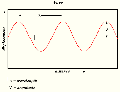
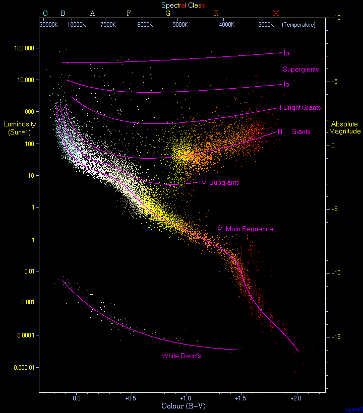
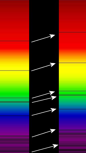
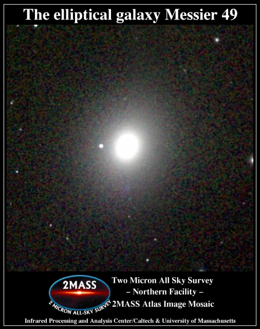
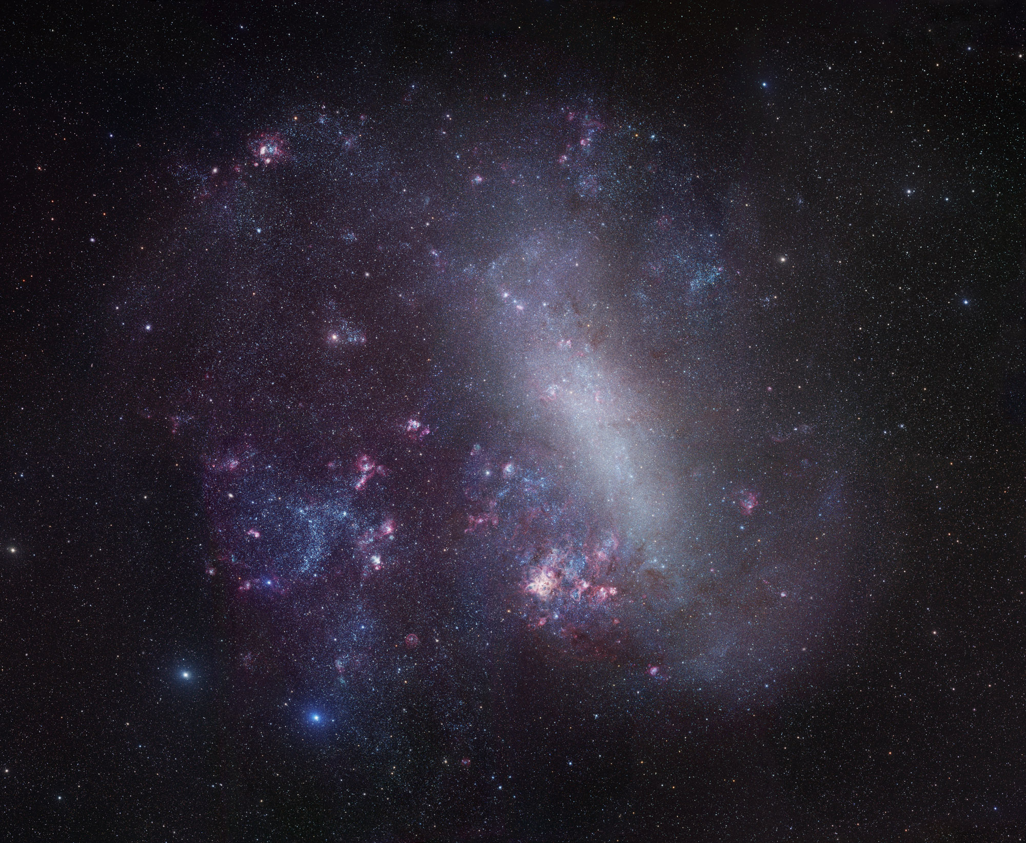
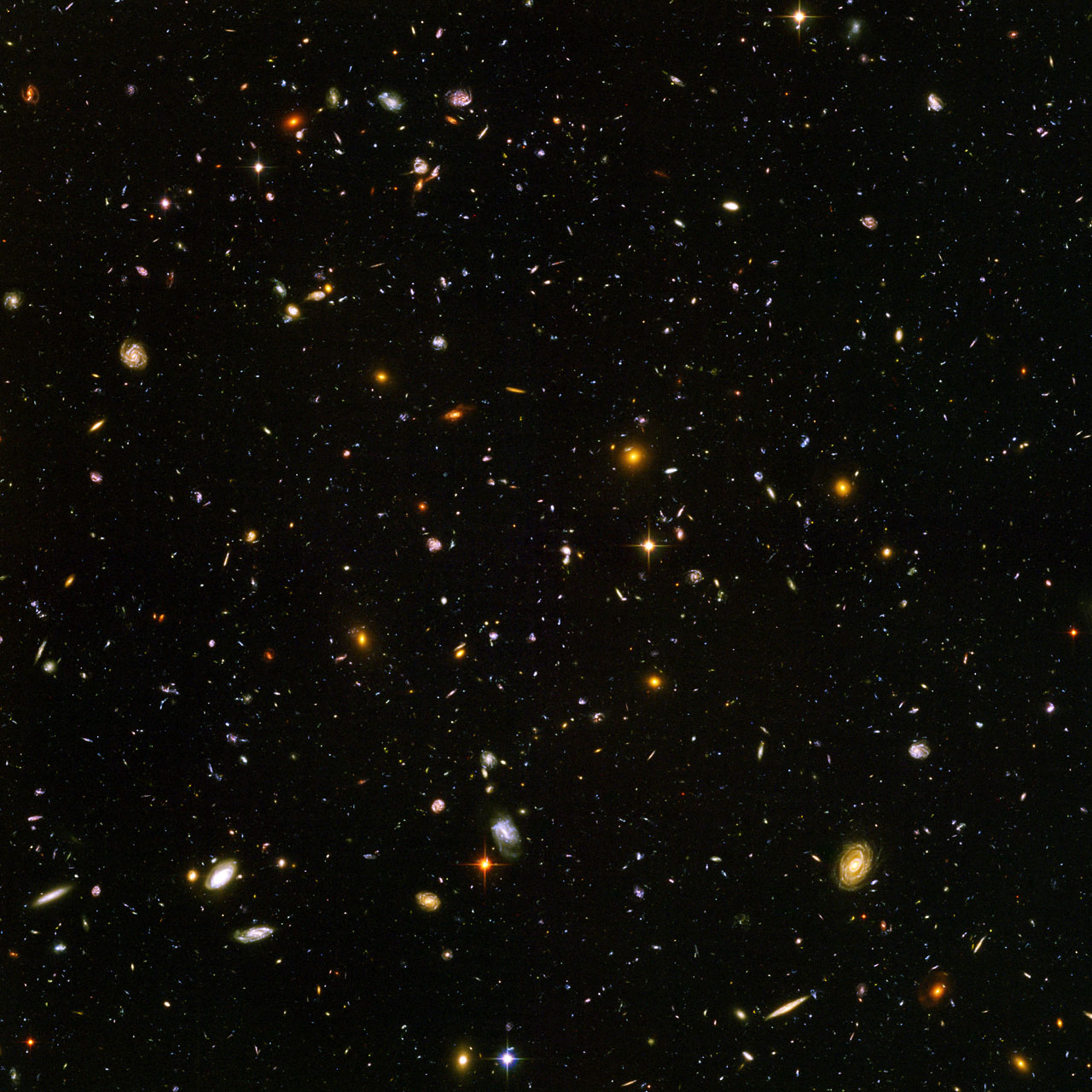
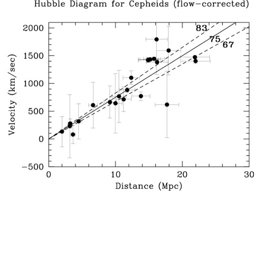
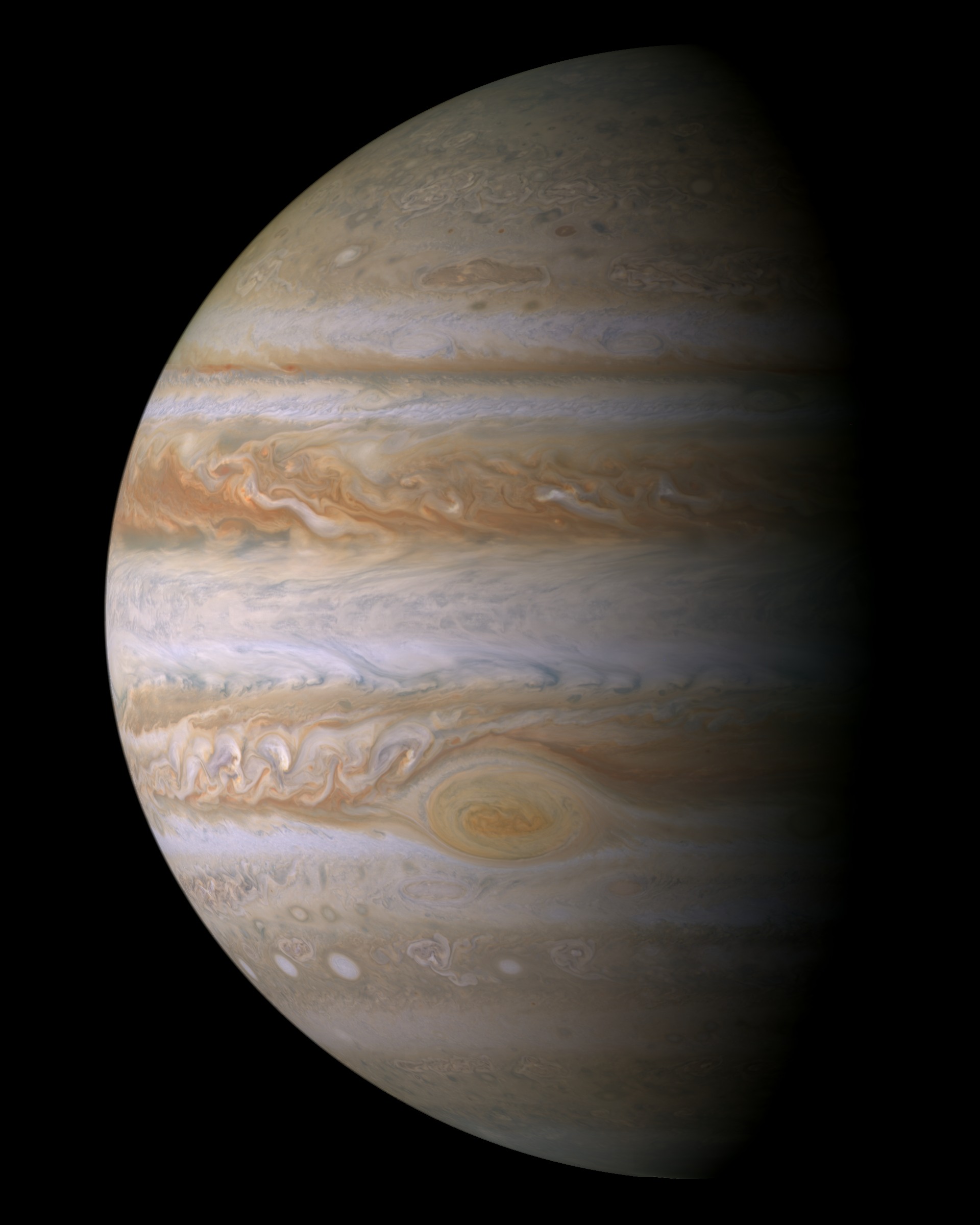
.png)
The exact origin of the Tunguska event is still unknown, although the evidence suggests that a meteor or comet exploded in the atmosphere before reaching Earth. There is no unambiguous crater left; however, trees for dozens of miles around the site were flattened by the explosion, which is estimated to have released energy equivalent to 15 or so megatons of TNT. Events of this size are expected statistically to occur on Earth approximately once a century. Larger impacts like the one that killed the dinosaurs are expected to occur about once every 50 million years. The largest impact on Earth since the Tunguska event was the Chelyabinsk meteor [683], which is estimated to have released energy equivalent to 500 kilotons of TNT in the atmosphere. To try to get some advanced warning of a potential impact, several efforts are underway to observe and catalog all of the Near Earth Objects (NEOs), that is, meteors and asteroids large enough to cause significant damage to Earth.
Want to learn more?
NASA has been charged by Congress to survey for NEOs and develop plans for diverting them from impacting the Earth. Information about the NASA program is available at the "Near Earth Object Program [684]" website. In particular, if you have heard about the potential for a collision between Earth and Apophis in 2029 or 2036, there is a comprehensive discussion [685]of this object there.
There is also a program called "SpaceWatch [686]" that is independently surveying for NEOs.
NASA has received some criticism for their work preparing for the diversion of any potentially hazardous asteroids. An organization called the "B612 Foundation [687]" is working on this independently.
The potential impact between Earth and a massive asteroid is one way in which our planet is in jeopardy from an astronomical phenomenon; but, unfortunately, it is not the only one. One of the other possibilities that we have to consider is the collision of the Earth with a molecular cloud of gas. The Earth's interaction with such a cloud is likely to destroy our atmosphere. The Earth may also lie in the path of the jet of emission from a gamma-ray burst, which will bombard the Earth with enough high energy radiation that there would again be catastrophic effects on the atmosphere. The rates of these events are also able to be estimated, and both appear to be 1 in 1 billion year type events.
Additional Resources
Below are some resources related to extrasolar planets and life in the Universe:
- There is an astrobiology curriculum [688] for middle and high school students published by TERC.
- The SETI Institute also has created an astrobiology curriculum called "Life in the Universe [689]"
- NASA Educator Resource Guides:
- NASA Kepler Mission planet finding activities [691]
- PBS has a Timothy Ferris movie called "Life Beyond Earth," and their website includes teacher resources [692].
- At Crash Course Astronomy [512], Phil Plait has episodes on Exoplanets (#27) and Life (#46)
Summary
What do you think? Are we alone? This is a fundamental question that everyone considers at some point. Now, we can say that we do know that other planets are prevalent in the Milky Way Galaxy and, given that result, perhaps it is likely that life is, too.
Activity 1 - Lesson 12 Quiz
Directions
First, please take the Web-based Lesson 12 quiz.
- Go to Canvas.
- Click on the link to the "Lesson 12 Quiz" and complete the quiz.
Good luck!
Activity 2 - Discussion
Directions
For this activity, I want you to reflect on what we've covered in this lesson and to discuss the threat related to Near Earth Objects. Since this is a discussion activity, you will need to enter the discussion forum more than once in order to read and respond to others' postings.
Submitting your work
- Enter the "NEOs" discussion forum in Canvas.
- Respond to the questions I have posted about NEOs.
- Read postings by other ASTRO 801 students.
- Respond to at least one other posting by asking for clarification, asking a follow-up question, expanding on what has already been said, etc.
Grading criteria
You will be graded on the quality of your participation. See the grading rubric [46] for specifics on how this assignment will be graded.
Reminder - Complete all of the lesson tasks!
You have finished the reading for Lesson 12. Double-check the list of requirements on the Lesson 12 Overview page to make sure you have completed all of the activities listed there before beginning the next lesson.
Capstone Project
Overview
My philosophy for the course and the project
This course is a true survey of astronomy. Although topics have been covered in some depth, in order to cover all of them, you have been referred to a host of additional resources that you may have investigated already or can follow up with after the course ends. You presented to each other additional resources that you find useful to help explain some of the concepts we covered in the course, too. In some cases, you were asked to discuss specifically how you teach some of the topics you studied in ASTRO 801.
This course was constructed by piecing together what I consider to be excellent resources available from NASA, other universities, Starry Night, and a few that I and my colleagues have created. I fully expect all of you to take what you find useful and incorporate those into your teaching.
I am not an expert in pedagogy at the K-12 level, but I have read some of the research and conducted my own on teaching and learning of astronomy. I have studied the PA state standards, the National Science Education Standards, and most recently the Framework for K-12 Science Education [693] and the Next Generation Science Standards. In particular, the NSES emphasizes the need for science teaching to increasingly rely on inquiry-based techniques, and the NGSS talks describe the integration of science practices and science content in the K-12 classroom. I have adopted many of these in my teaching, and when I teach face- to-face professional development workshops for teachers, I model inquiry-based activities and find these to be the most successful at transferring knowledge.
Given the emphasis on these types of pedagogies in most science methods courses at universities and in the education literature, I am going to focus our capstone activity on inquiry-based activities.
Capstone Project Overview
For this project, you will choose to develop one of the following:
- An inquiry-based classroom activity
- A laboratory exercise
- A detailed learning object (unless you are an experienced programmer, you will not submit a working learning object, but a storyboard for one)
Examples of each are provided on the next page.
The overall project will be broken up into three parts, presented on the next few pages.
- Part 1: Topic, Audience, & Project Type
- Part 2: Learning Objectives & Detailed Project Description
- Part 3: Final Project Report
Part 1: Topic, Audience, & Project Type
At the end of this project, you should have a written report that provides enough detail for you and your classmates to teach the content area that you have chosen. To begin to focus your project, I would like you to concentrate on these three areas:
- Topic
- Audience
- Project Type
Select a topic
Part of your grade will depend on how relevant your topic is to the content you have studied in this course. I would like you to choose a topic area that fits broadly into planets, stars, galaxies, and the Universe. You can choose a topic that we studied in depth, one that we covered briefly and you would like to study further, or one that we skipped, but still falls into the broad categories we studied.
Examples include:
- Stellar evolution: The proposed activity presents the stellar evolution of a Sun-like star in an innovative manner that is superior in some ways to the way we looked at it in this course.
- Black holes: The proposed activity presents the relativistic effects one would experience when encountering a black hole in more depth than it is presented in a previous lesson.
- The nature of blue stragglers: The proposed activity presents the stellar evolution of the type of stars known as blue stragglers, which are similar to, but different from any we studied in our lessons.
An example of a topic that I would consider not relevant to the course for this project is something related directly to human spaceflight in Earth orbit. For example, if you propose to focus your project on the growth of vegetables in the International Space Station to feed the astronauts, I would recommend you choose differently. However, if you want to talk about the nature of orbits and celestial mechanics by an investigation of how rockets get humans to the Moon and back, that is much more relevant and a good option for our project. If you are unsure if I would consider your topic relevant, please contact me for early feedback prior to submitting your work for Part 1.
Identify the audience
You should also focus your project to the audience. You are welcome to choose the audience you would like to work with, for example, you might choose:
- One class of 6th-grade students: If you teach 6th graders, you should certainly create a project that will work for you to teach your students!
- High school physics classes: You can create a project that is appropriate for students in high school physics classes, which may be a mix of ages of students, depending on the school.
- Informal education: Perhaps you work with out of school groups, such as scout troops, 4-H clubs, or robotics clubs. You can choose to design a project for these mixed age clubs that have different requirements and expectations than a formal classroom.
Choose a project type
In the overview, I specified that you could choose to create one of the following project types:
- An inquiry-based activity
- A laboratory exercise, or
- A learning object.
Clearly, these are not well-defined, non-overlapping categories, but again, for example, I consider the following:
- Inquiry-based activity: Kinesthetic Astronomy [694] teaches the 3D Sun / Earth orbital relationship by having students act out the Earth's orbit kinesthetically.
- Laboratory exercise: The SDSS HR Diagram lab [695] we completed has students create HR diagrams using real astronomical data.
- Learning object: The ClassAction Phases of the Moon module [75] is a set of learning objects that teachers can use to supplement classroom instruction on the phases of the Moon.
Activity
Directions
NOTE: You will be submitting your work as a single document that is in either Microsoft Word (.doc) or PDF (.pdf) format so I can open it. Try to keep your write-up for Part 1 to a page or a bit more than a page.
- Write a single statement that summarizes the topic your project will address (e.g., "My capstone project will follow the stellar evolution of a blue straggler star").
- Write a concise description (a paragraph or two) that presents the scientific content you need to cover to address the topic completely.
- Describe the audience you will be targeting and write a concise description of how you will focus your project to address the needs of that particular audience.
- In your write-up, tell me which option you are choosing, and provide a preliminary description of the outlines of your idea.
- Save your work AS A SINGLE DOCUMENT in either a Microsoft Word or PDF file in the following format:
CapstonePart1_AccessAccountID_LastName.doc (or .pdf).
For example, student Elvis Aaron Presley's file would be named "CapstonePart1_eap1_presley.doc" - This naming convention is important, as it will help me make sure I match each submission with the right student!
Submit your work
Please submit your work to the Capstone Project - Part 1 dropbox in Canvas by the due date indicated in our course calendar.
Grading criteria
You will not receive a separate grade for Part 1, as you will receive one grade on the overall project. However, I will be providing feedback on Part 1, so you will simply receive a check that I received your Part 1 submission by the deadline, which is typically mid-week during our work on Lesson 9.
Part 2: Learning Outcomes and a Detailed Project Description
Now that you have a topic, audience, and a project type chosen for your capstone project, you can refine your lesson by defining the specific learning outcomes that you want your audience to take away from your activity. Once you have your outcomes defined, the details of your project should be chosen so that audience members who perform the activity, do the lab, or use the learning object achieve those outcomes.
Defining learning outcomes
You have leeway within your chosen topic to define exactly what you want students to take away after completing the activity or lab or after using the learning object you are planning to describe. As you know from your education background, learning outcomes are statements that specify what learners will know or be able to do as a result of a learning activity. They are typically expressed as knowledge, skills, or attitudes.
In Part 1, I used a Kinesthetic Astronomy activity as an example. Let's also use it as an example for defining learning outcomes. If you download the lesson, a number of outcomes are stated, including:
- Demonstrate why we see different constellations in the night sky at different times of the year.
- Reason correctly in addressing the question of whether people in the US tonight will see the same stars that people in China saw last night (assuming everyone is observing from the same latitude).
Your learning outcomes should be stated as succinctly as the examples taken from that lesson. Furthermore, they should be measurable. A learning outcome that says, for example, that a student will "understand why we see different constellations in the night sky at different times of the year" doesn't indicate how one would know if that were achieved. It is too vague. The verb "demonstrate" does a better job of indicating how that outcome would be measured. (See more examples of action verbs for learning outcomes. [696])
Detailed project description
You should provide a project description that includes enough detail that someone else could replicate the activity, lab, or use of the learning object. Please use any template you are comfortable with or create your own document from scratch, but your description should include the following categories of information:
- A brief description of the background astronomy content that explains, in detail, what the students will actually do and how that addresses your science content area.
- A list of any materials they will need and instructions for using those materials to complete the activity, lab, or learning object.
- A description of what the students will deliver at the end of the activity, lab, or learning object (e.g., a lab report, a paper, etc.).
- A rubric that you will use to evaluate their work.
If you have chosen to create a learning object for your project, you should present a storyboard for that learning object to address #1 above. If you do not intend the students to directly interact with it (e.g., you will present it as an in-class demo), you should still describe what the students will do during the lesson that incorporates that learning object as an answer to #2 - 4 in the list above.
Activity
Directions
NOTE: You will be submitting your work as a single document that is in either Microsoft Word (.doc) or PDF (.pdf) format so I can open it. Try to keep your write-up for Part 2 to a reasonable length. I will not provide a strict page count, but think you should keep it succinct and only use the number of pages you find necessary to answer the questions above completely.
- Write several concise statements that summarize your learning outcomes.
- Write, using the template or format of your choosing, a detailed project description that addresses the four required parts listed above [description, materials & instructions, student deliverable(s), and your rubric].
- Save your work AS A SINGLE DOCUMENT in either a Microsoft Word or PDF file in the following format:
CapstonePart2_AccessAccountID_LastName.doc (or .pdf).
For example, student Elvis Aaron Presley's file would be named "CapstonePart2_eap1_presley.doc" - This naming convention is important, as it will help me make sure I match each submission with the right student!
Submit your work
Please submit your work to the Capstone Project - Part 2 dropbox in Canvas by the due date indicated on our course calendar.
Grading criteria
You will not receive a separate grade for Part 2, as you will receive one grade on the overall project. However, I will be providing feedback on Part 2, so you will simply receive a check that I received your Part 2 submission by the deadline, which is typically 3 weeks after Part 1 is due.
Part 3: Final Report
For this final part of the capstone project, I would like you to produce one last document that incorporates your previous two parts but also summarizes your overall vision for your new lesson. Your final report should include the following:
- Part 1—the topic, audience, and project type.
- Part 2—the detailed project description.
- Part 3—A detailed final summary of the project as a whole, which should include why it is appropriate for the audience you chose and your implementation plan (i.e., how you expect you or others might implement it).
The topics you should address in discussing the appropriateness for your audience might include:
- Does it address state or national standards for the grade level you chose?
- Is the project type appropriate for out of class time if you chose to create an activity for a club?
- Will the project fit naturally into the typical curriculum for a grade level?
During your discussion of your implementation plan, you should elaborate on your description from Part 2. For example, you might:
- Provide a scenario that describes how you would interact with your students as they undertake the project.
- Compare and contrast your project with a similar lesson you teach currently.
Your summary does not need to be long, but it does need to be complete and address both aspects described above. The final report should be a single, complete project that provides the reader all of the information and instruction necessary for the implementation of your project at their institution.
Activity
Directions
Note: You will be submitting your work as a single document that is in either Microsoft Word (.doc) or PDF (.pdf) format so I can open it. There is no minimum page limit, but I expect it should take at least one page to address the requirements for the summary.
- Copy and paste Part 1 and Part 2 into your final report.
- Edit those parts as necessary so that they flow into your final summary.
- Write the final summary as its own section.
- Save your work AS A SINGLE DOCUMENT in either a Microsoft Word or PDF file in the following format:
CapstonePart3_AccessAccountID_LastName.doc (or .pdf).
For example, student Elvis Aaron Presley's file would be named "CapstonePart3_eap1_presley.doc" - This naming convention is important, as it will help me make sure I match each submission with the right student!
Submit your work
Please submit your work to the Capstone Project - Part 3 dropbox in Canvas by the due date indicated on our course calendar, which is usually mid-week during finals week, three weeks after Part 2 is due.
Grading criteria
See the grading rubric [383] for specifics on how this assignment will be graded.
Additional Resources
Below are some resources related to the Capstone Project:
- The National Science Education Standards [697] include examples of the types of inquiry-based lessons that you may wish to describe in your project.
- Most of the resources that you have seen throughout the course are examples of the types of activities, labs, and learning objects that you can use for inspiration for your projects. However, let me list a few that I consider to be the best and that you can look at as exemplars:
- All of the Hubblesite "Amazing Space" online explorations [698]
- The Chandra Educational Materials classroom-ready activities [699]
- The Gettysburg CLEA laboratories [700]
- The ClassAction Modules [75]
- The Colorado PhET simulations [701]
- There are no online versions you can read, but I also recommend the GEMS guides "The Real Reasons for Seasons [702]" and "Invisible Universe [703]."
Tell us about it!
Have another website or printed piece on this topic that you have found useful? Share it in our Comment space below!
Links
[1] https://www.e-education.psu.edu/astro801/l1.html
[2] http://www.flickr.com/photos/vidiot/16725237/
[3] http://www.astronomynotes.com/nakedeye/chindex.htm
[4] http://www.astronomynotes.com/
[5] http://www.astronomynotes.com/nakedeye/s4.htm
[6] http://www.astronomynotes.com:
[7] http://www.astronomynotes.com/nakedeye/s5.htm
[8] http://www.astronomynotes.com/nakedeye/s6.htm
[9] http://antwrp.gsfc.nasa.gov/apod/ap030307.html
[10] http://www.astronomynotes.com/nakedeye/s7.htm
[11] http://commons.wikimedia.org/
[12] http://www.astronomynotes.com/nakedeye/s10.htm
[13] https://www.pbs.org/video/crash-course-astronomy-3/
[14] http://www.astronomynotes.com/nakedeye/s13.htm
[15] https://nam01.safelinks.protection.outlook.com/?url=https%3A%2F%2Fstock.adobe.com%2Fcontributor%2F204389456%2Fpandawild%3Fload_type%3Dauthor%26prev_url%3Ddetail&data=02%7C01%7Ceab14%40psu.edu%7C9e15cbe6cb414ff0256608d72d51cfe1%7C7cf48d453ddb4389a9c1c115526eb52e%7C0%7C0%7C637027701707904284&sdata=3OykUN57474%2Fe64w9Yu6OJ7WMARCLMIjFv1t6ZFAZyM%3D&reserved=0
[16] http://aa.usno.navy.mil/faq/docs/moon_phases.php
[17] https://astro.unl.edu/naap/lps/lunarPage2.html
[18] https://eclipse2017.nasa.gov/
[19] http://www.teachersdomain.org/resource/ess05.sci.ess.eiu.eclipse/
[20] http://apod.gsfc.nasa.gov/apod/ap031121.html
[21] http://apod.gsfc.nasa.gov/apod/ap010118.html
[22] http://apod.gsfc.nasa.gov/apod/ap030522.html
[23] http://apod.gsfc.nasa.gov/apod/ap990830.html
[24] http://apod.gsfc.nasa.gov/apod/ap021209.html
[25] http://apod.gsfc.nasa.gov/apod/ap021206.html
[26] https://apod.nasa.gov/apod/ap170825.html
[27] https://eclipse.gsfc.nasa.gov/SEgoogle/SEgoogle2001/SE2024Apr08Tgoogle.html
[28] http://apod.gsfc.nasa.gov/apod/ap970903.html
[29] https://apod.nasa.gov/apod/ap030605.html
[30] http://apod.nasa.gov/apod/astropix.html
[31] http://apod.nasa.gov/apod/ap030307.html
[32] http://apod.nasa.gov/apod/ap040829.html
[33] http://apod.nasa.gov/apod/ap031121.html
[34] http://apod.nasa.gov/apod/ap990830.html
[35] http://apod.nasa.gov/apod/ap080807.html
[36] http://hubblesite.org/
[37] http://www.spacescience.org/education/extra/kinesthetic_astronomy/index.html#dl
[38] http://www.lhs.berkeley.edu/starclock/skywheel.html
[39] http://www.stellarium.org/
[40] http://www.mreclipse.com/Special/SEprimer.html
[41] http://www.mreclipse.com/Special/LEprimer.html
[42] https://www.amep.com/index.php?route=product/product&product_id=923
[43] http://www.astronomynotes.com
[44] http://www.teachastronomy.com
[45] https://www.pearson.com/us/higher-education/program/Prather-Lecture-Tutorials-for-Introductory-Astronomy-3rd-Edition/PGM275203.html
[46] https://www.e-education.psu.edu/astro801/node/2077
[47] http://www.astronomynotes.com/nakedeye/s15.htm
[48] http://solar-center.stanford.edu/AO/sunrise.html
[49] https://www.e-education.psu.edu/astro801/sites/www.e-education.psu.edu.astro801/files/snf/Mars_prograde_2008.snf
[50] https://www.e-education.psu.edu/astro801/sites/www.e-education.psu.edu.astro801/files/snf/Mars_retrograde_2003.snf
[51] http://apod.gsfc.nasa.gov/apod/ap031216.html
[52] http://apod.gsfc.nasa.gov/apod/ap011220.html
[53] http://www.astronomynotes.com/scimethd/chindex.htm
[54] http://www.astronomynotes.com/scimethd/s2.htm
[55] http://www.astronomynotes.com/scimethd/s6.htm
[56] http://en.wikipedia.org/wiki/Occam%27s_razor
[57] http://www.windows.ucar.edu/tour/link=/the_universe/uts/eratosthenes_calc_earth_size.html
[58] http://www.astronomynotes.com/history/s3.htm
[59] http://www.astronomynotes.com/history/s4.htm#A3.3
[60] https://www.youtube.com/channel/UCw5d1S08MW2fqCdiJyfE8yw
[61] http://www.astronomynotes.com/history/s7.htm#A5
[62] http://en.wikipedia.org/wiki/File:Kepler-first-law.svg
[63] http://mathworld.wolfram.com/Ellipse.html
[64] http://en.wikipedia.org/wiki/Ellipse
[65] http://en.wikipedia.org/wiki/File:Drawing_an_ellipse_via_two_tacks_a_loop_and_a_pen.jpg
[66] http://en.wikipedia.org/wiki/File:Elps-slr.svg
[67] https://www.windows2universe.org/physical_science/physics/mechanics/orbit/eccentricity.html
[68] https://www.windows2universe.org/physical_science/physics/mechanics/orbit/ellipse.html
[69] http://phys23p.sl.psu.edu/phys_anim/astro/kepler_2.avi
[70] http://www.astronomynotes.com/gravappl/s2.htm
[71] http://www.astronomynotes.com/gravappl/s3.htm
[72] http://galileoandeinstein.physics.virginia.edu/more_stuff/flashlets/NewtMtn/home.html
[73] http://phet.colorado.edu/
[74] http://galileo.rice.edu/index.html
[75] http://astro.unl.edu/classaction/
[76] http://www.teachersdomain.org/resource/phy03.sci.ess.eiu.galMoon/
[77] http://www.teachersdomain.org/resource/phy03.sci.phys.mfw.zweightlessness/
[78] http://www.teachersdomain.org/resource/phy03.sci.phys.mfw.freefall/
[79] http://phet.colorado.edu
[80] http://essp.psu.edu/sites/default/files/tes_esspissue.pdf
[81] http://space.jpl.nasa.gov/
[82] https://cms.psu.edu/AngelUploads/QuestionData/cc6eeb06-6648-4638-bc76-b0deac9705d1/squigit_ruler.gif#%7BD7F8668A-4BA2-4B98-8781-E5C3CAF8532A%7D
[83] https://www.cluteinstitute.com/ojs/index.php/JAESE/article/view/9974
[84] http://www.astronomynotes.com/light/s2.htm
[85] http://www.astronomynotes.com/light/s3.htm
[86] http://en.wikipedia.org/wiki/File:2006-01-14_Surface_waves.jpg
[87] http://upload.wikimedia.org/wikipedia/commons/e/e9/Wave.png
[88] http://hubblesite.org
[89] http://amazing-space.stsci.edu/resources/explorations/light/
[90] https://www.americanscientist.org/article/herschel-and-the-puzzle-of-infrared
[91] https://www.youtube.com/watch?v=4M5vooCpai0
[92] https://public.nrao.edu/radio-astronomy/what-are-radio-waves/
[93] https://science.nasa.gov/ems/02_anatomy
[94] http://people.rit.edu/andpph/exhibit-spectrum.html
[95] http://www.noao.edu/image_gallery/images/d5/sunsqy.jpg
[96] http://imgsrc.hubblesite.org/hu/db/1997/35/images/e/formats/large_web.jpg
[97] http://voyages.sdss.org/preflight/light/spectra/
[98] http://mo-www.harvard.edu/Java/MiniSpectroscopy.html
[99] https://science.nasa.gov/ems
[100] https://science.nasa.gov/ems/05_radiowaves
[101] https://science.nasa.gov/ems/06_microwaves
[102] https://science.nasa.gov/ems/07_infraredwaves
[103] https://science.nasa.gov/ems/09_visiblelight
[104] https://science.nasa.gov/ems/10_ultravioletwaves
[105] https://science.nasa.gov/ems/11_xrays
[106] https://science.nasa.gov/ems/12_gammarays
[107] http://ccnmtl.columbia.edu/projects/helfand/
[108] https://www.youtube.com/watch?v=2--0q0XlQJ0
[109] https://www.e-education.psu.edu/astro801/sites/www.e-education.psu.edu.astro801/files/image/Lesson%203/Infrated_%20Astro801.docx
[110] http://www.spitzer.caltech.edu/images/2158-sig08-005-Hands-in-a-Bag-black-and-white-Visible-vs-Infrared-Light
[111] https://www.eso.org/public/images/atm_opacity/
[112] http://www.astronomynotes.com/light/s4.htm
[113] http://en.wikipedia.org/wiki/File:Wiens_law.svg
[114] https://phet.colorado.edu/en/simulation/blackbody-spectrum
[115] http://www.astronomynotes.com/light/s5.htm
[116] http://education.jlab.org/qa/atom_model.html
[117] http://phet.colorado.edu/simulations/sims.php?sim=Models_of_the_Hydrogen_Atom
[118] http://www.jce.divched.org/Journal/Issues/2006/May/abs761.html
[119] http://www.astronomynotes.com/telescop/s2.htm
[120] http://www.astronomynotes.com/telescop/s6.htm
[121] http://amazing-space.stsci.edu/resources/explorations/groundup/
[122] http://amazing-space.stsci.edu/resources/explorations/groundup/lesson/basics/index.php
[123] http://amazing-space.stsci.edu/resources/explorations/groundup/lesson/basics/g6/
[124] http://amazing-space.stsci.edu/resources/explorations/groundup/lesson/basics/g7/
[125] http://amazing-space.stsci.edu/resources/explorations/groundup/lesson/basics/g9a/
[126] http://amazing-space.stsci.edu/resources/explorations/groundup/lesson/basics/g4c/
[127] http://amazing-space.stsci.edu/resources/explorations/groundup/lesson/basics/g15/
[128] http://amazing-space.stsci.edu/resources/explorations/groundup/lesson/basics/g10areflector/
[129] http://amazing-space.stsci.edu/resources/explorations/groundup/lesson/basics/g28a/
[130] http://microscopy.berkeley.edu/courses/tlm/optics/spherical.html
[131] http://skyandtelescope.com/howto/scopes/article_241_2.asp
[132] https://history.aip.org/history/exhibits/cosmology/tools/tools-rebirth.htm
[133] http://www.astronomynotes.com/telescop/s10.htm
[134] http://www.astronomynotes.com/telescop/s11.htm
[135] http://www.astronomynotes.com/telescop/s12.htm
[136] http://spiff.rit.edu/classes/phys445/lectures/atmos/HIP4849.Film3.mov
[137] https://www.youtube.com/watch?v=sGf6wSQhz80
[138] http://phet.colorado.edu/simulations/sims.php?sim=Blackbody_Spectrum
[139] http://cas.sdss.org/dr7/en/proj/basic/color/physlet/blackbody.asp
[140] http://faraday.physics.utoronto.ca/PVB/Harrison/BohrModel/Flash/BohrModel.html
[141] http://chandra.harvard.edu/edu/chandra101.html
[142] http://coolcosmos.ipac.caltech.edu/cosmic_classroom/ir_tutorial/hist_index.html
[143] http://www.nrao.edu/index.php/learn/radioastronomy/radiotelescopes
[144] http://www.assumption.edu/users/bniece/Spectra/Contents.html
[145] http://www.pbs.org/seeinginthedark/
[146] http://www.pbs.org/seeinginthedark/for-teachers/
[147] http://www.slooh.com/home.php
[148] http://mo-www.harvard.edu/MicroObservatory/
[149] http://galileoscope.org/
[150] http://www.astronomynotes.com/starprop/s5.htm
[151] http://www.astronomynotes.com/starprop/s12.htm
[152] http://imgsrc.hubblesite.org/hu/db/2000/33/images/b/formats/full_jpg.jpg
[153] http://astron.berkeley.edu/%7Ebait/calstar/bear1.html
[154] http://hubble.stsci.edu/gallery/behind_the_pictures/meaning_of_color/
[155] http://hubble.stsci.edu/gallery/behind_the_pictures/meaning_of_color/filters.php
[156] http://www.wellesley.edu/Astronomy/Annie/
[157] http://www.noao.edu/
[158] http://www.astronomynotes.com/starprop/s2.htm#A1.1
[159] http://www.astronomy.ohio-state.edu/~pogge/Ast162/Movies/parallax.gif
[160] http://sci.esa.int/gaia/
[161] http://astronomy.as.virginia.edu/public-outreach/observatory-public-night-program
[162] http://www.astronomynotes.com/starprop/s3.htm
[163] http://commons.wikimedia.org/wiki/File:Inverse_square_law.svg
[164] http://www.astronomynotes.com/starprop/s4.htm
[165] http://curious.astro.cornell.edu/the-universe/82-the-universe/stars-and-star-clusters/measuring-the-stars/387-what-is-apparent-magnitude-intermediate
[166] https://www.windows2universe.org/the_universe/Stars/magnitude_scale.html
[167] http://www.astronomynotes.com/starprop/s13.htm
[168] http://www.phys-astro.sonoma.edu/BruceMedalists/Hertzsprung/index.html
[169] http://www.phys-astro.sonoma.edu/BruceMedalists/Russell/index.html
[170] http://upload.wikimedia.org/wikipedia/commons/6/6b/HRDiagram.png
[171] http://apod.gsfc.nasa.gov/apod/ap010223.html
[172] http://sci.esa.int/education/35774-stellar-radiation-stellar-types/?fbodylongid=1703
[173] http://stars.astro.illinois.edu/sow/hrd.html
[174] http://www.astronomynotes.com/light/s10.htm#A5
[175] http://www.astronomynotes.com/starprop/s8.htm
[176] http://astro.uchicago.edu/yerkes/outreach/activities/Explorations/BarnardsStar/barnards_star.mov
[177] http://en.wikipedia.org/wiki/File:Barnard2005.gif
[178] http://en.wikipedia.org/wiki/File:Doppler_effect.svg
[179] http://www.explorelearning.com/index.cfm?method=cResource.dspDetail&ResourceID=18
[180] http://www.lon-capa.org/~mmp/applist/doppler/d.htm
[181] http://www.astrocappella.com/background/doppler_background.shtml
[182] http://www.astrocappella.com/songs/doppler.mp3
[183] http://www.astrocappella.com/doppler.shtml
[184] http://upload.wikimedia.org/wikipedia/commons/1/14/Redshift.png
[185] http://www.acs.psu.edu/drussell/Demos/doppler/doppler.html
[186] https://pumas.gsfc.nasa.gov/examples/index.php?id=96
[187] http://stars.astro.illinois.edu/sow/sowlist.html
[188] http://cas.sdss.org/dr6/en/proj/basic/color/
[189] http://cas.sdss.org/dr6/en/proj/advanced/color/
[190] http://cas.sdss.org/dr6/en/proj/basic/spectraltypes/
[191] http://cas.sdss.org/dr6/en/proj/advanced/spectraltypes/
[192] http://www.astronomynotes.com/evolutn/s3.htm#A1.2.1
[193] http://www.astronomynotes.com/ismnotes/s3.htm#A1.2.1
[194] http://apod.gsfc.nasa.gov/apod/ap020530.html
[195] http://apod.gsfc.nasa.gov/apod/ap001229.html
[196] http://apod.gsfc.nasa.gov/apod/ap030202.html
[197] http://apod.gsfc.nasa.gov/apod/ap070425.html
[198] http://apod.gsfc.nasa.gov/apod/ap990301.html
[199] https://hubblesite.org/contents/news-releases/2007/news-2007-34.html?keyword=bok%20globule
[200] https://hubblesite.org/contents/news-releases/2015/news-2015-01.html?keyword=eagle%20nebula
[201] http://apod.gsfc.nasa.gov/apod/ap081009.html
[202] http://apod.gsfc.nasa.gov/apod/ap080918.html
[203] http://apod.gsfc.nasa.gov/apod/ap990509.html
[204] http://apod.gsfc.nasa.gov/apod/image/0109/barnard68_vlt_big.jpg
[205] http://www.eso.org/public/outreach/press-rel/pr-1999/phot-29a-99-normal.jpg
[206] http://hubblesite.org/newscenter/archive/releases/1995/44/image/a/format/web_print/
[207] http://www.pbs.org/wgbh/nova/origins/hubble.html
[208] http://www.astronomynotes.com/evolutn/s3.htm
[209] http://www.astronomynotes.com/evolutn/s4.htm
[210] http://apod.gsfc.nasa.gov/apod/ap080719.html
[211] http://phet.colorado.edu/simulations/sims.php?sim=Gas_Properties
[212] https://www.youtube.com/watch?v=tmNXKqeUtJM
[213] http://hubblesite.org/gallery/album/entire_collection/pr2001013b/
[214] http://imgsrc.hubblesite.org/hu/db/1995/24/images/a/formats/web_print.jpg
[215] http://www.astronomynotes.com/starsun/s3.htm
[216] http://www.astronomynotes.com/evolutn/s5.htm#A1.2.6
[217] http://www.astronomynotes.com/evolutn/s7.htm
[218] http://www.astronomynotes.com/starsun/s4.htm
[219] http://apod.gsfc.nasa.gov/apod/ap071213.html
[220] http://commons.wikimedia.org/wiki/File:FusionintheSun.svg
[221] http://www.bnl.gov/bnlweb/history/Nobel/Nobel_02.asp
[222] http://www.bnl.gov/bnlweb/raydavis/Default.htm
[223] http://www.astronomynotes.com/evolutn/s2.htm#A1.1
[224] http://www.astronomynotes.com/starsun/s8.htm#A5.6
[225] http://hubblesite.org/newscenter/archive/releases/1995/48/image/a/
[226] http://hubblesite.org/newscenter/archive/releases/2006/31/full/
[227] http://www.science.psu.edu/news-and-events/2006-news/Luhman9-2006-2.htm/
[228] http://science.psu.edu/news-and-events/2013-news/Luhman3-2013
[229] http://www.astronomynotes.com/starprop/s10.htm
[230] http://www.astronomynotes.com/starprop/s11.htm
[231] http://antwrp.gsfc.nasa.gov/apod/ap001006.html
[232] http://www.astronomy.ohio-state.edu/~pogge/Ast162/Movies/specbin.html
[233] http://www.astronomy.ohio-state.edu/~pogge/Ast162/Movies/eclbin.html
[234] http://imgsrc.hubblesite.org/hu/gallery/db/video/starslife/formats/starslife_640x480.mov
[235] https://www.nasa.gov/content/hubble-traveling-exhibit-stars
[236] http://chandra.harvard.edu/edu/formal/stellar_ev/
[237] http://articles.adsabs.harvard.edu/cgi-bin/nph-iarticle_query?bibcode=1914PA.....22..275R&db_key=AST&page_ind=10&data_type=GIF&type=SCREEN_VIEW&classic=YES&high=4995bd2e6f17161
[238] http://iopscience.iop.org/article/10.1086/301326/fulltext/fg1.h.jpg
[239] http://cas.sdss.org/dr7/en/proj/advanced/hr/
[240] http://www.astronomynotes.com/evolutn/s5.htm
[241] http://upload.wikimedia.org/wikipedia/commons/7/7c/Sun_red_giant.svg
[242] http://hubblesite.org/newscenter/archive/releases/1996/04/image/a/format/web_print/
[243] http://www.astronomynotes.com/evolutn/s5.htm#A1.2.7
[244] http://www.astronomynotes.com/evolutn/s10.htm
[245] ftp://sohoftp.nascom.nasa.gov/pub/oldwww/explore/DynSun.html
[246] http://www.astronomynotes.com/evolutn/s6.htm
[247] http://www.astronomynotes.com/evolutn/s6.htm#A1.2.9
[248] http://chandra.harvard.edu/about/chandra.html
[249] http://www.cfa.harvard.edu/news/archive/pr0407.html
[250] http://hubblesite.org/newscenter/archive/releases/star%20cluster/2002/10/image/a/
[251] http://hubblesite.org/newscenter/archive/releases/1999/01/image/a/format/large_web/
[252] http://pearljam.com/music/albums/997/studio/18623/binaural
[253] https://hubblesite.org/contents/news-releases/2004/news-2004-27.html
[254] https://hubblesite.org/contents/news-releases/2004/news-2004-11.html
[255] https://hubblesite.org/contents/news-releases/2004/news-2004-32.html
[256] https://hubblesite.org/contents/news-releases/2011/news-2011-38.html
[257] https://hubblesite.org/contents/media/images/2000/07/940-Image.html
[258] https://hubblesite.org/contents/media/images/2000/28/990-Image.html
[259] https://hubblesite.org/video/64/news/34-planetary-nebulas
[260] http://hubblesite.org/newscenter/archive/releases/2001/05/video/b/
[261] http://www.aao.gov.au/images.html/captions/aat048.html
[262] http://hubblesite.org/newscenter/newsdesk/archive/releases/1995/49/image/a
[263] https://hubblesite.org/contents/media/images/1999/04/756-Image.html
[264] http://chandra.harvard.edu/resources/animations/hd_anim.html
[265] http://www.astronomynotes.com/evolutn/s11.htm#A2.3
[266] http://map.gsfc.nasa.gov/mission/observatory_l2.html
[267] http://www.jwst.nasa.gov/orbit.html
[268] http://www.haydenplanetarium.org/tyson/read/2002/04/01/the-five-points-of-lagrange
[269] http://en.wikipedia.org/wiki/File:RochePotential.jpg
[270] http://chandra.harvard.edu/resources/animations/mira.mov
[271] https://www.youtube.com/watch?v=xAjq7VGnf4s
[272] http://demonstrations.wolfram.com/ContactBinaryStarEnvelopes/
[273] http://hubblesite.org/newscenter/archive/releases/star/multiple%20star%20systems/1995/23/image/a/
[274] http://hubblesite.org/newscenter/archive/releases/1997/29/
[275] http://antwrp.gsfc.nasa.gov/apod/ap990524.html
[276] http://www.skyandtelescope.com/astronomy-news/observing-news/supernova-in-m82-passes-its-peak/
[277] http://www.astronomynotes.com/evolutn/s12.htm
[278] http://hubblesite.org/newscenter/archive/releases/1997/32/image/a/format/web_print/
[279] https://chandra.si.edu/photo/2013/vela/animations.html
[280] http://www.jb.man.ac.uk/~pulsar/Education/Sounds/sounds.html
[281] http://www.bigear.org/vol1no1/burnell.htm
[282] https://vimeo.com/37312387
[283] http://antwrp.gsfc.nasa.gov/apod/ap050721.html
[284] http://www.nasa.gov/centers/goddard/mpg/97799main_Millisec%20Pulsar%20Shot%201.mpg
[285] https://www.nobelprize.org/prizes/physics/1993/press-release/
[286] http://www.nasa.gov/centers/goddard/news/topstory/2003/0702pulsarspeed.html
[287] http://lisa.nasa.gov/index.html
[288] http://cgwp.gravity.psu.edu/outreach/
[289] http://www.astronomynotes.com/evolutn/s13.htm
[290] http://www.astro.psu.edu/users/niel/astro130/astro130.html
[291] http://blogs.discovermagazine.com/badastronomy/2008/10/30/ten-things-you-dont-know-about-black-holes/
[292] http://www.astronomynotes.com/relativity/s3.htm
[293] http://antwrp.gsfc.nasa.gov/htmltest/rjn_bht.html
[294] https://www.youtube.com/watch?v=h1iJXOUMJpg
[295] http://www.phy.mtu.edu/bht/bh_pub_faq.html
[296] http://cosmology.berkeley.edu/Education/BHfaq.html
[297] http://www.spacetelescope.org/images/html/cygx1_illustration_orig.html
[298] http://hubble.stsci.edu/explore_astronomy/black_holes/home.html
[299] http://hubblesite.org/hubble_discoveries/hstexhibit/stars/
[300] http://chandra.harvard.edu/edu/formal/stellar_ev/poster_horiz_med2.jpg
[301] http://chandra.harvard.edu/edu/request.html
[302] http://imagine.gsfc.nasa.gov/teachers/lifecycles/stars.html
[303] http://imagine.gsfc.nasa.gov/teachers/blackholes/blackholes.html
[304] http://imagine.gsfc.nasa.gov/teachers/elements/elements.html
[305] http://imagine.gsfc.nasa.gov/teachers/index.html
[306] http://xmm.sonoma.edu/edu/supernova/
[307] http://fermi.sonoma.edu/teachers/blackholes/index.php
[308] http://hubblesite.org/newscenter/archive/releases/2004/20/image/a/
[309] http://apod.gsfc.nasa.gov/apod/ap071122.html
[310] http://apod.gsfc.nasa.gov/apod/ap060109.html
[311] http://apod.gsfc.nasa.gov/apod/ap050103.html
[312] https://www.subaru.com.au/about/the-pleiades-constellation%20
[313] http://antwrp.gsfc.nasa.gov/apod/ap010909.html
[314] http://www.noao.edu/image_gallery/html/im0379.html
[315] http://www.noao.edu/image_gallery/html/im0423.html
[316] http://www.noao.edu/image_gallery/html/im0552.html
[317] http://hubblesite.org/newscenter/archive/releases/2001/22/image/e
[318] http://www.noao.edu/image_gallery/html/im0838.html
[319] http://www.noao.edu/image_gallery/html/im0551.html
[320] http://www.noao.edu/image_gallery/html/im0836.html
[321] http://messier.seds.org/
[322] http://spider.seds.org/ngc/ngc.html
[323] http://www.ipac.caltech.edu/2mass/
[324] http://www.sdss.org/
[325] http://www.ipac.caltech.edu/2mass/releases/allsky/doc/sec1_8a.html
[326] https://www.atnf.csiro.au/outreach//education/senior/astrophysics/stellarevolution_mainsequence.html
[327] http://www.astro.ulb.ac.be/~siess/pmwiki/pmwiki.php/WWWTools/Isochrones
[328] http://en.wikipedia.org/wiki/File:Isochrone_ZAMS_Z2pct.png
[329] http://www.cfa.harvard.edu/news/archive/pr0424.html
[330] https://www.e-education.psu.edu/astro801/sites/www.e-education.psu.edu.astro801/files/snf/MilkyWay_MessierObjects.snf
[331] http://www.noao.edu/image_gallery/images/d2/02215.jpg
[332] http://www.sns.ias.edu/~starlab/animations/
[333] http://www.astronomynotes.com/evolutn/s9.htm
[334] http://outreach.atnf.csiro.au/education/senior/astrophysics/stellarevolution_clusters.html
[335] http://csep10.phys.utk.edu/astr162/index.html
[336] http://www.astronomynotes.com/ismnotes/s5.htm
[337] http://commons.wikimedia.org/wiki/File:HR-diag-instability-strip.svg
[338] http://www.pbs.org/wgbh/aso/databank/entries/baleav.html
[339] http://apod.nasa.gov/apod/ap981027.html
[340] http://www.astrosociety.org/education/astronomy-resource-guides/women-in-astronomy-an-introductory-resource-guide/
[341] http://history.amazingspace.org/resources/organizers/starclusters.php
[342] http://www.aavso.org/
[343] https://youtu.be/an4rgJ3O21A
[344] http://cas.sdss.org/dr7/en/proj/advanced/hr/neareststars.asp
[345] http://cas.sdss.org/dr7/en/proj/advanced/hr/mast.asp
[346] https://www.e-education.psu.edu/astro801/node/2079
[347] http://www.nps.gov/deva/naturescience/lightscape.htm
[348] http://apod.gsfc.nasa.gov/apod/ap070508.html
[349] http://apod.gsfc.nasa.gov/apod/ap090219.html
[350] http://apod.gsfc.nasa.gov/apod/ap090127.html
[351] http://apod.gsfc.nasa.gov/apod/ap010627.html
[352] http://www.ipac.caltech.edu/2mass/gallery/showcase/galcen/Galactic_Cntr_full.jpg
[353] http://www.ipac.caltech.edu/2mass/gallery/showcase/galcen/index.html
[354] http://en.wikipedia.org/wiki/File:Aitoff-projection.jpg
[355] http://apod.gsfc.nasa.gov/apod/ap980523.html
[356] http://apod.gsfc.nasa.gov/apod/ap990426.html
[357] http://apod.gsfc.nasa.gov/apod/ap010202.html
[358] http://apod.gsfc.nasa.gov/apod/ap011020.html
[359] http://www.ipac.caltech.edu/2mass/gallery/showcase/allsky/index.html
[360] http://www.astronomynotes.com/ismnotes/s2.htm#A1.1.1
[361] http://articles.adsabs.harvard.edu/full/1922ApJ....55..302K
[362] http://hubblesite.org/newscenter/archive/releases/2002/01/image/a/
[363] http://www.astronomynotes.com/ismnotes/s6.htm
[364] http://www.haydenplanetarium.org/universe
[365] http://www.astronomynotes.com/ismnotes/s4.htm
[366] http://www.astronomynotes.com/ismnotes/s9.htm
[367] http://www.spitzer.caltech.edu/images/1925-ssc2008-10b-A-Roadmap-to-the-Milky-Way-Annotated-
[368] http://mwmw.gsfc.nasa.gov/mmw_edu.html
[369] http:=
[370] http://mwmw.gsfc.nasa.gov/mmw_MW.html
[371] http://mwmw.gsfc.nasa.gov/mmw_maps.html
[372] http://www.astronomynotes.com/ismnotes/s9.htm#A2.7
[373] http://www.nrl.navy.mil/media/news-releases/1998/wide-field-radio-imaging-of-the-galactic-center
[374] http://apod.gsfc.nasa.gov/apod/ap020803.html
[375] http://chandra.harvard.edu/press/01_releases/press_020101.html
[376] http://images.nrao.edu/Galactic_Sources/Galactic_Center/407
[377] http://www.astro.ucla.edu/~ghezgroup/gc/animations.html
[378] http://www.astronomynotes.com/ismnotes/s7.htm
[379] http://en.wikipedia.org/wiki/Galaxy_rotation_curve
[380] http://chandra.harvard.edu/xray_astro/navigation.html
[381] http://chandra.harvard.edu/resources/illustrations/milkyWay.html
[382] http://chandra.harvard.edu/photo/2003/0203long/animations.html
[383] https://www.e-education.psu.edu/astro801/node/2078
[384] http://www.astronomynotes.com/galaxy/s2.htm
[385] http://articles.adsabs.harvard.edu/cgi-bin/nph-iarticle_query?bibcode=1910ApJ....32...26R&db_key=AST&page_ind=10&plate_select=NO&data_type=GIF&type=SCREEN_GIF&classic=YES&high=49beb5749119894
[386] http://antwrp.gsfc.nasa.gov/diamond_jubilee/debate20.html
[387] http://apod.gsfc.nasa.gov/apod/ap960406.html
[388] http://www.aip.org/history/cosmology/index.htm
[389] http://www.aip.org/history/exhibits/cosmology/ideas/island.htm
[390] https://www.aip.org/history/exhibits/cosmology/ideas/larger-image-pages/pic-island-notebook.htm
[391] https://www.aip.org/history/exhibits/cosmology/ideas/larger-image-pages/pic-island-m31.htm
[392] http://antwrp.gsfc.nasa.gov/diamond_jubilee/1996/sandage_hubble.html
[393] https://thecosmos4.com/
[394] http://www.astronomynotes.com/galaxy/s3.htm
[395] http://www.astronomynotes.com/galaxy/s4.htm
[396] http://www.astronomynotes.com/galaxy/s5.htm
[397] http://hubblesite.org/newscenter/archive/releases/1999/34/image/o/format/large_web/
[398] http://www.spitzer.caltech.edu/uploaded_files/images/0008/1211/sig07-025_Med.jpg
[399] http://www.spitzer.caltech.edu/images/2095-sig07-025-Lifestyles-of-the-Galaxies-Next-Door
[400] http://www.spitzer.caltech.edu/uploaded_files/images/0008/1186/sig07-025.tif
[401] https://hubblesite.org/video/881/tours
[402] https://hubblesite.org/video/887/tours
[403] https://hubblesite.org/video/886/tours
[404] http://www.noao.edu/image_gallery/images/d4/m81y.jpg
[405] http://apod.gsfc.nasa.gov/apod/ap020710.html
[406] http://www.eso.org/public/images/eso9921a/
[407] https://www.noao.edu/image_gallery/images/d6/m95_2.jpg
[408] http://apod.gsfc.nasa.gov/apod/image/0304/ngc1365_vlt_big.jpg
[409] https://www.noao.edu/image_gallery/images/d6/m61.jpg
[410] https://www.noao.edu/image_gallery/images/d6/m87i.jpg
[411] http://www.ipac.caltech.edu/2mass/gallery/m49atlas.jpg
[412] http://www.noao.edu/image_gallery/images/d6/m59.jpg
[413] http://www.noao.edu/image_gallery/images/d4/m82a.jpg
[414] http://apod.gsfc.nasa.gov/apod/image/0812/LMCmosaicM_gendler.jpg
[415] https://www.noao.edu/image_gallery/galaxies.html
[416] http://hubblesite.org/gallery/album/galaxy/pr2003028a/
[417] http://www.noao.edu/outreach/aop/observers/n4565.html
[418] http://commons.wikimedia.org/wiki/File:Football_on_ground.jpg
[419] http://apod.gsfc.nasa.gov/apod/ap080913.html
[420] http://apod.gsfc.nasa.gov/apod/ap080124.html
[421] http://apod.gsfc.nasa.gov/apod/ap080909.html
[422] http://www.astronomynotes.com/galaxy/s12.htm
[423] http://www.astronomynotes.com/galaxy/s13.htm
[424] http://www.astronomynotes.com/galaxy/s14.htm
[425] http://hubblesite.org/newscenter/archive/releases/1996/01/text/
[426] http://cas.sdss.org/dr7/en/tools/explore/obj.asp?id=587722982271090881
[427] http://cas.sdss.org/dr7/en/tools/explore/obj.asp?id=588015507682230507
[428] http://cas.sdss.org/dr7/en/tools/explore/obj.asp?id=587731513690095801
[429] http://hubblesite.org/newscenter/archive/releases/1998/28/image/a/
[430] http://images.nrao.edu/132
[431] http://images.nrao.edu/56
[432] http://images.nrao.edu/110
[433] http://apod.gsfc.nasa.gov/apod/ap060704.html
[434] http://skyserver.sdss.org/dr7/en/tools/explore/obj.asp?id=587725074457821263
[435] http://skyserver.sdss.org/dr7/en/tools/explore/obj.asp?id=587725074995019808
[436] http://cas.sdss.org/astro/en/tools/getimg/plate.asp
[437] http://apod.gsfc.nasa.gov/apod/ap031128.html
[438] http://www.npr.org/sections/thetwo-way/2016/02/23/467826553/solving-the-mystery-of-the-disappearing-quasar
[439] http://www.astronomynotes.com/galaxy/s9.htm
[440] http://apod.gsfc.nasa.gov/apod/ap060806.html
[441] http://antwrp.gsfc.nasa.gov/apod/ap050213.html
[442] http://antwrp.gsfc.nasa.gov/apod/ap010126.html
[443] http://www.astronomynotes.com/galaxy/s10.htm#A2.9.1
[444] http://hubblesite.org/gallery/album/entire/pr1997034a/
[445] http://hubblesite.org/newscenter/archive/releases/2002/11/video/a/
[446] http://hubblesite.org/newscenter/archive/releases/2008/16/video/d/
[447] http://hubblesite.org/news_release/news/1997-34
[448] http://hubblesite.org/video/122/news_release/1997-34
[449] https://hubblesite.org/contents/media/videos/2002/11/883-Video.html
[450] http://burro.astr.cwru.edu/models/models.html
[451] https://www.youtube.com/watch?v=QcDtJ_-jdMw
[452] http://www.astro.virginia.edu/~mfs4n/sgr/
[453] http://hubblesite.org/newscenter/archive/releases/2002/11/image/a/
[454] http://apod.gsfc.nasa.gov/apod/ap080207.html
[455] http://apod.gsfc.nasa.gov/apod/ap080619.html
[456] http://apod.gsfc.nasa.gov/apod/ap980831.html
[457] https://hubblesite.org/contents/news-releases/1997/news-1997-02.html
[458] http://www.astronomynotes.com/galaxy/s10.htm
[459] http://www.sdss.org/signature.html
[460] http://hubblesite.org/newscenter/archive/releases/2004/07/
[461] http://hubblesite.org/newscenter/archive/releases/2004/07/image/i/
[462] http://www.astronomynotes.com/galaxy/s16.htm
[463] http://fermi.sonoma.edu/teachers/agn.php
[464] http://www.galex.caltech.edu/education/teachers.html
[465] http://www.galaxyzoo.org/
[466] http://voyages.sdss.org/
[467] http://voyages.sdss.org/galaxy-shapes/
[468] https://youtu.be/I82ADyJC7wE
[469] https://youtu.be/_O2sg-PGhEg
[470] http://www.spacetelescope.org/static/archives/images/screen/heic0406a.jpg
[471] http://www.aip.de/groups/galaxies/sw/udf/swudfV1.0.html
[472] http://en.wikipedia.org/wiki/File:Biogradska_suma.jpg
[473] https://commons.wikimedia.org/wiki/Category:Olbers%27_paradox#/media/File:Olber%27s_Paradox_-_All_Points.gif
[474] http://hubblesite.org/gallery/album/the_universe/pr2006012b/large_web/
[475] http://en.wikipedia.org/wiki/Olbers_paradox
[476] http://www.astronomynotes.com/cosmolgy/s2.htm#A1.3
[477] http://www.pnas.org/content/15/3/168
[478] http://adsabs.harvard.edu/abstract_service.html
[479] http://hubblesite.org/newscenter/archive/releases/1999/19/text/
[480] http://nedwww.ipac.caltech.edu/level5/Sept01/Freedman/Figures/figure1.jpg
[481] http://www.astronomynotes.com/cosmolgy/s3.htm#A1.5
[482] http://map.gsfc.nasa.gov/universe/bb_tests_exp.html
[483] http://www.astronomynotes.com/cosmolgy/s3.htm
[484] http://www.astronomynotes.com/galaxy/s9.htm#A2.8
[485] http://hubblesite.org/newscenter/archive/releases/2008/24/image/e/format/large_web/
[486] http://apod.gsfc.nasa.gov/apod/ap041025.html
[487] http://www.astronomy.ohio-state.edu/~dhw/SDSS08/ofigs.html
[488] http://apod.nasa.gov/apod/ap010904.html
[489] http://www.pnas.org/content/96/9/4756/F1.large.jpg
[490] http://www.astronomynotes.com/cosmolgy/s9.htm
[491] http://map.gsfc.nasa.gov/universe/bb_concepts.html
[492] http://www.astronomynotes.com/cosmolgy/s5.htm
[493] https://aas.org/files/resources/An_Ancient_Universe.pdf
[494] http://map.gsfc.nasa.gov/universe/bb_tests_cmb.html
[495] http://lambda.gsfc.nasa.gov/product/cobe/cobe_image_table.cfm
[496] http://map.gsfc.nasa.gov/media/ContentMedia/990004b.jpg
[497] http://map.gsfc.nasa.gov/media/080997/index.html
[498] http://www.pbs.org/wgbh/aso/databank/entries/dp65co.html
[499] https://www.bell-labs.com/about/history-bell-labs/stories-changed-world/Cosmic-Microwave-Background-Discovery/
[500] http://www.nasa.gov/vision/universe/starsgalaxies/nobel_prize_mather.html
[501] http://www.lbl.gov/Publications/Nobel/
[502] http://www.astronomynotes.com/cosmolgy/s10.htm#A2.4
[503] http://www.astronomynotes.com/cosmolgy/s12.htm#A3.2
[504] http://hubblesite.org/newscenter/archive/releases/2008/08/image/b/
[505] http://www.cfa.harvard.edu/supernova//home.html
[506] http://map.gsfc.nasa.gov/media/080998/index.html
[507] http://map.gsfc.nasa.gov/universe/
[508] http://www.astronomynotes.com/cosmolgy/chindex.htm
[509] http://www.astro.psu.edu/users/niel/psiwa-2006-cosmology/psiwa.html
[510] http://map.gsfc.nasa.gov/resources/edactivity2.html
[511] https://www.astro.princeton.edu/~dns/teachersguide/teachersguide.html
[512] https://www.youtube.com/playlist?list=PL8dPuuaLjXtPAJr1ysd5yGIyiSFuh0mIL
[513] http://www.astronomynotes.com/solarsys/s3.htm
[514] http://www.astronomynotes.com/solarsys/s8b.htm#A7
[515] http://www.astronomynotes.com/solarsys/s8.htm
[516] http://www.astronomynotes.com/solarsys/s11.htm
[517] https://www.sciencebase.gov/catalog/item/51dda464e4b0f72b4471e1f5
[518] http://apod.gsfc.nasa.gov/apod/ap050101.html
[519] http://earth.google.com/
[520] http://www.passc.net/EarthImpactDatabase/
[521] http://www.google.com/moon/
[522] http://news.psu.edu/story/317841/2014/06/09/research/55-year-old-dark-side-moon-mystery-solved
[523] http://photojournal.jpl.nasa.gov/catalog/PIA00302
[524] http://lunar.gsfc.nasa.gov/gallery-historical.html
[525] http://en.wikipedia.org/wiki/File:Full_Moon_Luc_Viatour.jpg
[526] http://apod.gsfc.nasa.gov/apod/ap981008.html
[527] http://www.history.com/shows/the-universe/videos/creation-of-the-moon
[528] http://www.astronomynotes.com/gravappl/s10.htm
[529] http://en.wikipedia.org/wiki/File:The_Earth_seen_from_Apollo_17.jpg
[530] http://en.wikipedia.org/wiki/File:Field_tidal.png
[531] http://oceanservice.noaa.gov/education/kits/tides/media/supp_tide06a.html
[532] http://oceanservice.noaa.gov/education/kits/tides/welcome.html
[533] http://en.wikipedia.org/wiki/Tides
[534] http://www.astronomynotes.com/solarsys/s9.htm
[535] http://www.astronomynotes.com/solarsys/s10.htm
[536] http://www.nineplanets.org/
[537] http://solarsystem.nasa.gov/planets/
[538] http://messenger.jhuapl.edu/
[539] http://www2.jpl.nasa.gov/magellan/
[540] http://hubblesite.org/gallery/album/solar_system/pr2003022a/large_web/
[541] http://eoimages.gsfc.nasa.gov/ve/2429/globe_west_540.jpg
[542] http://apod.gsfc.nasa.gov/apod/image/0311/jupiterp_cassini_full.jpg
[543] http://antwrp.gsfc.nasa.gov/apod/ap001123.html
[544] https://www.nasa.gov/mission_pages/juno/main/index.html
[545] http://antwrp.gsfc.nasa.gov/apod/ap960827.html
[546] http://antwrp.gsfc.nasa.gov/apod/ap020205.html
[547] http://heritage.stsci.edu/1999/29/index.html
[548] http://www.astronomynotes.com/solarsys/s16.htm
[549] http://apod.gsfc.nasa.gov/apod/ap041225.html
[550] http://hubblesite.org/newscenter/newsdesk/archive/releases/1996/16/image/a
[551] http://antwrp.gsfc.nasa.gov/apod/ap040723.html
[552] https://hubblesite.org/contents/media/images/1990/11/11-Image.html?news=true
[553] https://hubblesite.org/contents/media/images/2003/23/1392-Image.html
[554] http://hubblesite.org/newscenter/newsdesk/archive/releases/2004/05/
[555] http://antwrp.gsfc.nasa.gov/apod/ap010821.html
[556] https://hubblesite.org/image/1451/category/86-uranus
[557] http://www.astronomynotes.com/solarsys/s14.htm
[558] http://www.astronomynotes.com/solarsys/s15.htm
[559] http://apod.gsfc.nasa.gov/apod/ap971121.html
[560] http://apod.gsfc.nasa.gov/apod/ap971126.html
[561] http://photojournal.jpl.nasa.gov/catalog/?IDNumber=PIA01493
[562] http://www.nasa.gov/mission_pages/cassini/media/cassini-20090303.html
[563] http://www.astronomy.com/news/2017/06/jupiters-new-moons
[564] http://apod.gsfc.nasa.gov/apod/ap001118.html
[565] http://apod.gsfc.nasa.gov/apod/ap040502.html
[566] http://apod.gsfc.nasa.gov/apod/ap000606.html
[567] http://apod.gsfc.nasa.gov/apod/ap030919.html
[568] http://apod.gsfc.nasa.gov/apod/ap021101.html
[569] http://apod.gsfc.nasa.gov/apod/ap001020.html
[570] http://apod.gsfc.nasa.gov/apod/ap000620.html
[571] http://apod.gsfc.nasa.gov/apod/ap001218.html
[572] http://apod.gsfc.nasa.gov/apod/ap020120.html
[573] http://apod.gsfc.nasa.gov/apod/ap980512.html
[574] https://sites.google.com/carnegiescience.edu/sheppard/moons
[575] http://apod.gsfc.nasa.gov/apod/ap990207.html
[576] http://apod.gsfc.nasa.gov/apod/ap070207.html
[577] http://apod.gsfc.nasa.gov/apod/ap050224.html
[578] http://apod.gsfc.nasa.gov/apod/ap050215.html
[579] http://apod.gsfc.nasa.gov/apod/ap050201.html
[580] http://apod.gsfc.nasa.gov/apod/ap041201.html
[581] http://apod.gsfc.nasa.gov/apod/ap041129.html
[582] http://apod.gsfc.nasa.gov/apod/ap041217.html
[583] http://apod.gsfc.nasa.gov/apod/ap991010.html
[584] http://www.astronomynotes.com/solfluf/s8.htm
[585] http://press.princeton.edu/titles/8247.html
[586] http://www.gps.caltech.edu/~mbrown/howikilled.html
[587] http://www.nasa.gov/mission_pages/newhorizons/main/index.html
[588] http://hubblesite.org/newscenter/archive/releases/2003/2003/22/image/
[589] http://hubblesite.org/newscenter/newsdesk/archive/releases/1994/17/image/a
[590] http://hubblesite.org/newscenter/newsdesk/archive/releases/1996/09/image/a
[591] http://www.nasa.gov/mission_pages/newhorizons/images/index.html
[592] http://web.gps.caltech.edu/~mbrown/dps.html
[593] https://commons.wikimedia.org/wiki/File:10_Largest_Trans-Neptunian_objects_(TNOS).png
[594] http://www2.ess.ucla.edu/~jewitt/kb.html
[595] http://www.chadtrujillo.com/quaoar/
[596] https://hubblesite.org/contents/media/images/2002/17/1226-Image.html
[597] http://antwrp.gsfc.nasa.gov/apod/ap021009.html
[598] https://www.caltech.edu/news/caltech-researchers-find-evidence-real-ninth-planet-49523
[599] http://www.planetary.org/multimedia/space-images/charts/every-round-object-under-10k-2015.html
[600] http://apod.nasa.gov/apod/ap130708.html
[601] http://apod.nasa.gov/apod/ap151026.html
[602] http://hubblesite.org/gallery/album/pr2006029b
[603] http://www.iau.org/public/pluto/
[604] http://www.gps.caltech.edu/~mbrown/planetlila/
[605] http://www.astronomynotes.com/solfluf/s7.htm
[606] http://www.astronomynotes.com/solfluf/s9.htm
[607] http://antwrp.gsfc.nasa.gov/apod/ap001227.html
[608] http://apod.nasa.gov/apod/ap160202.html
[609] http://antwrp.gsfc.nasa.gov/apod/ap040512.html
[610] http://apod.gsfc.nasa.gov/apod/ap040724.html
[611] http://apod.nasa.gov/apod/ap090723.html
[612] http://hubblesite.org/newscenter/archive/releases/1994/21/image/b/
[613] http://www.windows2universe.org/comets/comet_model_interactive.html
[614] http://www.gps.caltech.edu/~mbrown/sedna/
[615] http://hubblesite.org/newscenter/newsdesk/archive/releases/1994/30/
[616] http://hubblesite.org/newscenter/newsdesk/archive/releases/1994/34/
[617] http://antwrp.gsfc.nasa.gov/apod/ap011215.html
[618] http://apod.gsfc.nasa.gov/apod/ap040630.html
[619] http://www.astronomynotes.com/solfluf/s2.htm
[620] http://www.astronomynotes.com/solfluf/s3.htm
[621] http://meteorite.unm.edu/meteorites/meteorite-museum/how-id-meteorite/
[622] http://apod.gsfc.nasa.gov/apod/ap050121.html
[623] http://apod.gsfc.nasa.gov/apod/ap970816.html
[624] http://en.wikipedia.org/wiki/File:Allende_meteorite.jpg
[625] http://www.lpi.usra.edu/science/kring/epo_web/meteorites/intro.html
[626] http://meteorites.asu.edu/outreach
[627] http://apod.gsfc.nasa.gov/apod/ap990711.html
[628] http://apod.gsfc.nasa.gov/apod/ap000226.html
[629] http://antwrp.gsfc.nasa.gov/apod/ap000226.html
[630] http://mars.jpl.nasa.gov/mro/
[631] http://antwrp.gsfc.nasa.gov/apod/ap040619.html
[632] http://www.astronomynotes.com/solfluf/s11.htm
[633] https://www.e-education.psu.edu/astro801/content/l5_p3.html
[634] https://youtu.be/BiIh_r-KTGM
[635] https://www.bbc.co.uk/programmes/p006x4v3
[636] http://mars.jpl.nasa.gov/
[637] http://marsed.asu.edu/stem-lesson-plans
[638] http://saturn.jpl.nasa.gov/index.cfm
[639] https://www.jpl.nasa.gov/edu/teach/tag/search/Cassini+Mission
[640] http://solarsystem.nasa.gov/ssa/home.cfm
[641] https://www.nasa.gov/mission_pages/newhorizons/main/index.html
[642] http://lunar.gsfc.nasa.gov/teacherresources.html
[643] http://exoplanets.org/
[644] http://exoplanets.org/plots
[645] http://apod.nasa.gov/apod/ap110329.html
[646] http://www.astronomynotes.com/solarsys/s10.htm#A2.2.1
[647] http://www.astronomynotes.com/lifezone/s3.htm
[648] http://astrobiology.nasa.gov/
[649] http://mpfwww.jpl.nasa.gov/mgs/newsroom/20061206b.html
[650] http://phoenix.lpl.arizona.edu/index.php
[651] http://mars.jpl.nasa.gov/programmissions/missions/
[652] http://phoenix.lpl.arizona.edu/exhibit.php
[653] https://solarsystem.nasa.gov/missions/galileo/overview/
[654] https://www.nasa.gov/feature/the-mysterious-lakes-on-saturns-moon-titan
[655] http://www.astronomynotes.com/solfluf/s12.htm
[656] https://exoplanets.nasa.gov/news/204/will-the-real-first-exoplanet-please-stand-up/
[657] http://exoplanet.eu/
[658] http://exoplanets.org
[659] http://planetquest.jpl.nasa.gov/index.cfm
[660] https://exoplanets.nasa.gov/5-ways-to-find-a-planet/
[661] https://www.e-education.psu.edu/astro801/content/l5_p6.html
[662] https://www.youtube.com/watch?v=ibCdL3MZCXQ&feature=youtu.be
[663] http://www.gemini.edu/sunstarplanet
[664] http://www.astronomynotes.com/lifezone/s2.htm
[665] https://en.wikipedia.org/wiki/Circumstellar_habitable_zone
[666] http://kepler.nasa.gov/multimedia/artwork/diagrams/?ImageID=29
[667] http://www.geosc.psu.edu/~kasting/PersonalPage/ResInt2.htm
[668] http://www3.geosc.psu.edu/~ruk15/planets/Seff_HZ_09032015.jpg
[669] http://www.astronomynotes.com/lifezone/s5.htm
[670] http://www.pbs.org/lifebeyondearth/listening/drake.html
[671] http://www.astronomynotes.com/lifezone/s6.htm
[672] http://www.bigear.org/6equj5.htm
[673] https://www.seti.org/
[674] https://www.seti.org/seti-research
[675] http://www.seti.org/seti-institute/project/details/sci-fi-movies
[676] http://sites.psu.edu/astrowright/the-g-hat-search-for-kardashev-civilizations/
[677] http://www.theatlantic.com/science/archive/2015/10/the-most-interesting-star-in-our-galaxy/410023/
[678] https://www.youtube.com/watch?v=_lqXc2ungX0
[679] http://mola.gsfc.nasa.gov/
[680] http://en.wikipedia.org/wiki/File:Hellas_basin_topo.jpg
[681] http://saturn.jpl.nasa.gov/science/moons/mimas/
[682] http://en.wikipedia.org/wiki/File:Tunguska_event_fallen_trees.jpg
[683] http://www.slate.com/blogs/bad_astronomy/2014/02/14/chelyabinsk_asteroid_impact_one_year_later.html
[684] http://neo.jpl.nasa.gov/index.html
[685] http://neo.jpl.nasa.gov/apophis/
[686] http://spacewatch.lpl.arizona.edu/
[687] http://b612foundation.org/
[688] https://www.terc.edu/terc_products/astrobiology-an-integrated-science-approach/
[689] https://www.seti.org/life-universe-litu-curriculum-files
[690] http://nai.nasa.gov/media/medialibrary/2013/10/Astrobiology-Educator-Guide-2007.pdf
[691] http://kepler.nasa.gov/education/
[692] http://www.pbs.org/lifebeyondearth/index.html
[693] http://www.nap.edu/catalog/13165/a-framework-for-k-12-science-education-practices-crosscutting-concepts
[694] http://www.spacescience.org/education/extra/kinesthetic_astronomy/index.html
[695] http://cas.sdss.org/dr5/en/proj/teachers/advanced/hr/
[696] https://www.e-education.psu.edu/astro801/sites/www.e-education.psu.edu.astro801/files/Blooms_ActionVerbs.pdf
[697] http://www.nap.edu/openbook.php?record_id=4962
[698] http://amazing-space.stsci.edu/resources/explorations/
[699] http://chandra.harvard.edu/edu/formal/index.html
[700] http://www3.gettysburg.edu/~marschal/clea/CLEAhome.html
[701] http://phet.colorado.edu/index.php
[702] http://www.lawrencehallofscience.org/gems/GEMSSeasons.html
[703] http://www.lawrencehallofscience.org/gems/gemsInvUniv.html