Lessons
This is the course outline.
Unit 1: Fresh Water: Scarcity or Surfeit?
Unit 1: Fresh Water: Scarcity or Surfeit?
Overview
Water is often called the “Elixir of Life.” We refer to Earth as the “Blue Planet” because of its abundance of liquid water; indeed, NASA’s search for life on other planets starts with the search for water. While its importance for sustaining life is perhaps common knowledge, the extent to which we depend on water in every aspect of our everyday lives and activities is less obvious. In this course, we will explore these facets of water’s impact on human society. We begin with an overview and discussion of the underpinnings of water use, occurrence, and movement. We then explore the many and profound consequences of human manipulation of water; the ability to reroute, store and transport water is one of the very things that has allowed human civilizations to thrive, yet has also led directly to a complex and broad-ranging relationship with this most essential of substances. Water pervades almost every aspect of our existence, including food production; the manufacture of goods and development of new technologies; transportation and energy generation; human health via its use for sanitation, the conveyance of waste, and control on the distribution of water-borne diseases; and the sustenance of ecosystems on which we often depend but do not realize. Not only is water needed for you to be here and to produce your breakfast this morning, but the computer you are using to read this course’s modules, the electricity needed to turn on your computer, the steel and fuel needed to transport you to/from school all required even more water!
Through its importance in these areas, it is perhaps unsurprising that water allocation and policy lie at the heart of economic and political tensions between communities, states, and nations. As populations in many water-stressed areas continue to grow, and in the face of climate changes that affect where and when water may be available in the future, these challenges continue to mount.
We begin this course by providing an outline of water resources on a global basis—where resources are abundant or limited and why. We first ask questions regarding the "value" of water and consider whether having access to fresh (uncontaminated) water for drinking and other household uses is a fundamental right as opposed to water being a commodity subject to profit-taking. In other words, is water a resource that is subject to privatizations and price fluctuations, or should water be provided by benevolent governments at a reasonable cost? In addition, we are concerned with projected population growth, its regional distribution, and resulting demands for water in the future. This helps us appreciate the two-way relationship between water and human society: how water availability and quality affect economic opportunities and human well-being, and how human activity affects water resources.
A major consideration is why some regions have a surplus of water and others have less than necessary to support local populations in various activities. In order to understand this, we need to examine the operation of Earth's climate system in some detail: the roles of global wind systems, proximity to an ocean, and topographic features (especially mountain belts) in determining patterns of rainfall, a first-order control on water availability. This involves discussion of the global "hydrologic cycle" that reflects the cycling of water from the ocean to atmosphere to land and its ultimate return to the sea. We also outline some of the important properties of water that determine its behavior in the climate system, flowing water, and sustaining life.
Modules
Unit Goals
Upon completion of Unit 1 students will be able to:
- Describe the two-way relationship between water resources and human society
- Explain the distribution and dynamics of water at the surface and in the subsurface of the Earth
- Interpret graphical representations of scientific data
- Identify strategies and best practices to decrease water stress and increase water quality
- Communicate scientific information in terms that can be understood by the general public
- Predict how the availability of and demand for water resources is expected to change over the next 50 years
Unit Objectives
In order to reach these goals, the instructors have established the following learning objectives for student learning. In working through the modules within Unit 1 students will be able to:
- List the primary reasons that most population centers developed near major rivers or other surface water bodies.
- Provide examples of consumptive and non-consumptive, and direct and indirect water uses.
- Compare the amounts used by the various end-users of water, both in the U.S. and globally.
- Identify regions of critical water stress at present and those anticipated 20 and 40 years into the future.
- Identify possible solutions to anticipated water shortages.
- Discuss issues surrounding the debate about public access to (clean) freshwater.
- Identify the unique physical properties of water that contribute to its fundamental role in driving Earth Systems.
- Quantitatively compare fluxes of water in the hydrologic cycle.
- Assess the relationship between precipitation, topography, and location in the U.S. and globally.
Module 1: Freshwater Resources - A Global Perspective
Module 1: Freshwater Resources - A Global Perspective
While only just beginning this course, you likely already appreciate that water is a precious commodity. For example, a human can survive at least three weeks without food, but can go only about three days without drinking water (or water-based liquid) before dehydration becomes a medical emergency (see the U.S. National Library of Medicines article, Water in Diet [3]. Nonetheless, in the U.S., we commonly take access to quality drinking water for granted, not to mention the availability of water for all other important activities including the production of food and energy. And, this water presently comes to most people in the U.S. at a very low cost—just cents per gallon. We are, of course, privileged relative to other regions of the world, some of which do not have sufficient fresh water resources and where people may not even have access to safe drinking water supplies.
In this module, we will examine the distribution of freshwater resources, the major uses of water, and present and anticipated future demand for water, globally, as the human population increases. We will explore the question as to whether water has a value greater than presently appreciated and whether it will always be readily available to us. For example, you may already know that the western U.S. is experiencing a severe shortage of water as the result of prolonged drought in that region. Is this an anomaly, or might we expect longer-term shortages there and elsewhere in the U.S. and globally as the result of climate change?
Goals and Objectives
Goals and Objectives
Goals
- Describe the two-way relationship between water resources and human society
- Explain the distribution and dynamics of water at the surface and in the subsurface of the Earth
- Communicate scientific information in terms that can be understood by the general public
- Interpret graphical representations of scientific data
- Identify strategies and best practices to decrease water stress and increase water quality
- Predict how availability of and demand for water resources is expected to change over the next 50 years
Learning Objectives
In completing this module, you will:
- Analyze the relationship between land use and access to fresh water
- Calculate the population that can be supported by a finite water source
- Evaluate possible solutions to anticipated water shortages
- Evaluate whether access to clean water is a basic human right, or if it should be treated as a commodity
- Distinguish between direct and indirect water use
- Record and analyze your own personal water usage
- Compare your own personal water use habits with those of your peers and others worldwide
The Value of Water
The Value of Water
Does water have value?
Water is essential to life – both as a basic human need for survival and as an “ingredient” in almost everything we do, from food production to manufacturing to power generation. As we will explore in more detail in Module 2 next week, precipitation and evaporation – and thus water availability – are unevenly distributed around the globe (Figure 1). This also varies seasonally. Figure 1 shows the average global distribution of precipitation for January; to see an animation over the course of the year, check this out:

There are obviously some areas of the world that are wetter than others, and these patterns are persistent throughout the year (i.e. the deserts of the American southwest, Northern Africa, and Western Australia are perennially dry; whereas equatorial central America, Africa, and Indonesia are wet). This uneven distribution of water resources lies at the root of many topics we’ll cover in this course, because it is a primary driver of human activity, ranging from population dynamics to types and locations of particular industries, to power generation, to politics. For example, take a look at the maps in Figures 1 and 2. Are there areas of the world that are persistently wetter or drier than others?


Activate Your Learning
1. List 3 areas/regions that are persistently dry based on the animated map shown above.
2. List 3 areas/regions that are persistently wet.
3. Inspect the freshwater availability map shown in Figure 2. Provide 2 examples of areas of water scarcity that “map” to areas where precipitation is low.
4. Identify 2 areas that are characterized by low precipitation, but apparently are not faced with severe water scarcity. Provide a hypothesis as to why you think this is the case.
As we’ll see in Module 2, water is transported around the Earth by the hydrologic cycle, in which solar energy drives evaporation of water from the oceans and land surface. This water condenses in the atmosphere to form clouds and eventually to fall as precipitation. Much of that precipitation flows as surface water in rivers and streams. Some of it also infiltrates or percolates into the soil and rock, and becomes groundwater. Surface water constitutes the primary source of water for human activity – it is relatively clean, easy to obtain and move, and constantly replenished (barring prolonged dry periods; as we will discuss in Modules 4 and 8-9). Groundwater constitutes another important source of water for human activity. Although the total volume of groundwater held in fractures and pore spaces in the subsurface is large, it is replenished and flows under natural conditions far more slowly than surface water. Additional energy is required to extract groundwater, because it must be pumped from the subsurface, in some cases hundreds of feet or more. For these reasons, groundwater is generally a secondary source of water, in cases where surface water is not readily available or cannot fully meet demand.
Food for Thought
List at least 2 problems or issues (these can be political, economic, health-related, etc…) that might arise from the unequal geographic distribution of water resources.
Global Freshwater Resources
Global Freshwater Resources
Water use and treatment
Once taken for human use, water generally follows a path described in Figure 3 below. After undergoing treatment and distribution, it is used. In the broadest sense, water is constantly being re-used. Water that is taken from rivers or streams for domestic, industrial, or agricultural use was most likely also used by communities or farms up-stream, and subsequently treated and discharged. Over even longer timescales, the water in streams, lakes, and groundwater is the same water that has ever been on Earth – and those same molecules have undoubtedly cycled through many plants and animals before we were even around!
Depending on the nature of water use, it may be re-captured after treatment (“recycled water”) for re-use. As we will see later in the semester, this re-use of water resources is one strategy to cope with water scarcity. The recycled water, depending on its quality, can be used for irrigation (i.e. for parks or golf courses), or for domestic supply. Once the water leaves the “use” loop, it is treated and discharged, typically into surface water bodies. In some cases, the treated water may be used to recharge aquifers instead, either through induced recharge systems or at a smaller scale via passive filtration through soils – for example in leachfields. The discharged water, after mixing with water in the river, stream (or aquifer), becomes a water source for downstream or down-gradient users.

Activate Your Learning
1. Do you know the source of domestic or municipal water in your hometown? If yes, what and where is it? If no, does it surprise you to realize that you don't know where your drinking water comes from?
2. Do you suppose that any of that water is used and then treated by others before being taken for your use?
3. Take a look at figure 3 above. Had you thought about your water as a substance that has a “life cycle” and is constantly being used, treated, released, and re-used? If not, does the idea make you uncomfortable?
Water and Population Centers
Water and Population Centers
Some cities are sited in areas where water is available - or was at the time they were settled - including Las Vegas, Los Angeles, Chicago, St. Louis, and Pittsburgh (Figure 4). In some cases, and as we will discuss in detail in later modules in the course, rapid development and growing demand can outpace the original and limited water source for a city or region, leading to a vicious cycle of water acquisition, growth enabled by water availability, and subsequent water stress.


Many of America’s major manufacturing centers (i.e. the rust belt) are located in areas where major rivers and canals provided a means for transport of raw materials and goods, power generation, water supply for processing and cooling, and conveyance of waste. At small scale, harnessing hydropower was accomplished by mills; at larger scales in modern dams, it is through hydroelectric power generation. Major rivers also provide the water supply for irrigation-based agriculture in some areas, where precipitation is not sufficient or consistent enough to support crops.

Indeed, for these reasons, rivers in many parts of the world are considered the “lifeblood” of society (Figure 6). For example, the Nile River valley in Egypt comprises ~5% of the land area, yet is home to nearly the entire population of 78 million, with a population density among the highest in the world (more than 1000 people per square km). Despite the obvious connection between water availability and human needs, the story of water resource distribution and population growth is not that simple! In some cases, major engineering projects in which millions of acre-feet of water are moved across states or continents have allowed cities and irrigated agricultural regions to flourish in water-scarce parts of the world. In others, major dams or new water sources (i.e. deep groundwater, reclaimed water, or desalination) have provided a means for cities to prosper in unlikely places. For example, take another look at Figure 4 above. The concentration of nighttime lights provides a reasonable proxy for population density. In many parts of the U.S., they follow the water: along the St. Lawrence, girdling the Great Lakes, and along the Mississippi River. Yet other major population centers have sprung up in perennially dry regions, mainly in the deserts of the southwest: Los Angeles, Las Vegas, Tucson, and Albuquerque.
Learning Checkpoints
1. Inspect Figures 4 and 5 and compare the two maps. Note 3 major cities that are near large water sources (rivers or lakes). View Figures 4 and 5above.
2. List 3 cities or regions of high population density that are not near major water sources, and/or lie in areas of low precipitation.
3. Do you know anyone who lives in one of these dry areas, or have you thought about moving there?
Water Quality and Human Health
Water Quality and Human Health
The distribution of water-rich and water-poor regions is of course not the whole story – access to clean water isn’t just about the amount of water that falls as precipitation. It’s also about the infrastructure needed to obtain, treat, transport, and deliver potable water. And that’s just the water supply. Disposal and sanitation of dirty water are equally important and require a means of transporting waste away from the distributed sources, collecting it and treating it, and discharging it safely. Ideally, both supply and waste conveyance systems should also be monitored for performance and for their impacts on water quality.
In some areas, water is plentiful, but access to clean water is not (Figures 7-8). The converse is also true, mainly in developed nations where water projects, desalination, or dams provide a water supply to regions that receive little precipitation. There is also a clear distinction between access to clean water in rural and urban areas (Figure 7), wherein access in rural areas, even in developed nations, lags behind that in urban areas.

| Year | Status | Water Supply | Improved Sanitation |
|---|---|---|---|
| 1990 | World | 95% | 79% |
| 1990 | Developing | 92% | 61% |
| 2004 | World | 96% | 80% |
| 2004 | Developing | 91% | 70% |
| Year | Status | Water Supply | Improved Sanitation |
|---|---|---|---|
| 1990 | World | 63% | 26% |
| 1990 | Developing | 61% | 19% |
| 2004 | World | 72% | 39% |
| 2004 | Developing | 70% | 35% |
Learning Checkpoint
1. What is the primary trend shown in Figure 7 above, with respect to urban vs. rural areas?
2. Is there a major difference in access to clean water supply and sanitation when comparing developed and developing nations?
3. Which is the bigger difference – urban vs. rural, or developed vs. developing nations?
4. Do you find your answer to question #3 surprising – or is it what you had expected?
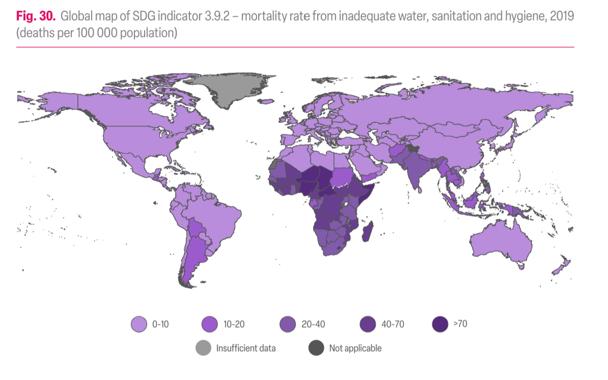
Access to clean water differs between rural and urban areas, and between developed and developing nations. In general, in rural areas, even in developed nations, access to water and sanitation lags behind that in urban areas. Globally, the areas with the poorest access to clean drinking water are in equatorial and sub-Saharan Africa, and parts of South America and southeast Asia (Figure 8).
One might imagine that access to clean water and sanitation would be strongly correlated with water-related illnesses and death. For example, compare the maps in Figures 8 and 9.

Learning Checkpoint
1. Compare the maps in Figures 8 and 9. Is there a correlation between access to improved water and water-related illness? Note two areas where there is a correlation, either positive or negative. See Figures 8 and 9 above.
2. Based on Figure 8 and the distribution of water availability, do you think that these problems are related to water scarcity, or more related to water treatment and infrastructure?
Water Usage: What and Where?
Water Usage: What and Where?
How much water do we use, and for what? Water “permeates” almost every aspect of our lives (no pun intended!). Some uses of water are obvious – for example, municipal and domestic supply used for drinking, cleaning, flushing and watering. Others are less obvious, such as water used for irrigation to grow produce, grains, or feed. The water needed to raise livestock is one step further removed, since the water “used” to produce the product includes the water that must go into growing feed. Yet other uses of water are even less visible, for example for refining fuels, cooling for thermo-electric power generation, and the manufacturing of almost everything in our day-to-day lives.;
Because the types and scales of water use vary widely – from domestic wells that pump at a few gallons per minute, to allocations of major rivers in billions of gallons, the units of measurement used for water management also span an enormous range (see Units).
Water Use
Water Use
How much and for what purposes?
Globally, there is a widely varied usage of water, as a result of differing total populations and population densities, geography and climate (i.e. water availability), cultures, economies, lifestyles, and water use and reuse efficiency. This can be described both in terms of total water abstraction from surface water and groundwater sources and as per capita water withdrawal. It can also be divided to consider the end uses (for example, as percentages of the total use), or to consider the source of the water. Each of these facets of water use illuminates different aspects of the “water story”.
In many industrialized nations, the dominant water uses are for industry (including thermoelectric power generation, manufacturing, etc…) and agriculture (Figures 10-11). In contrast, domestic and municipal water use generally constitutes less than 15-30% of the total. In developing nations, this is somewhat different – total water use is smaller, less is used for industry, and the proportion used for domestic water supply is larger.
In the U.S., the average per capita use of domestic or municipal water (i.e. the most direct uses – those that would be measured by the water meter at your home) is about 215 m3 per person per year, equivalent to 156 gallons per day (as of 2002). For comparison, the total abstraction of water from surface and groundwater sources in the U.S. is about 1700 m3/person/yr, or 1230 gallons per day. The difference in these numbers represents the large proportion of water that goes to so-called “indirect” uses: food production, manufacturing, power generation, and mining, among others.
In contrast, in sub-Saharan Africa, total water use is less than 200 m3 per person per year (less than 12% of water use in the U.S.). Total abstractions in Western Europe are about 600 m3 per person per year, about 850 m3 per person per year in the Middle East; and 1150 m3 per person per year in Australia. Among those nations with the highest water use, agriculture accounts for anywhere from <40% of use (U.S.), to 67-81% (India and China), to as much as 96% (Pakistan). Industrial use (including power generation) ranges from over 80% of total water use to less 1%. In the U.S. water use for power generation is near 50%; in China, it constitutes 25% and in India about 5%. Germany, Russia, Canada, France, and much of Western Europe use around 60% of withdrawn water for power generation. Municipal and domestic water use typically constitutes about 10-20% of the total and varies little among the worlds most populous countries (Figure 9). You can explore these patterns on your own via a useful interactive plotting engine at Gapminder. [11]
It is important to note that because many products are imported or exported across state and national borders, the total abstractions of water in a given place do not necessarily map to the distribution of water “consumption” there. Consider tomatoes that are transported from California to Massachusetts. The water withdrawal from rivers and aquifers needed to grow the tomatoes would appear on California’s “water tab”, but the eventual use of that water would be elsewhere. The same goes for agricultural and industrial products exported internationally. This flow of indirectly used water, embedded in products, is termed virtual water, and is defined as the amount of water used in generation of the product, or alternatively, the amount of water that would be needed to generate the product at the site where it is ultimately used. It is “virtual” because the water use is indirect; it is required to make or grow the item but is not actually physically contained in the item or transported with it.
Consumptive vs. Non-consumptive Use
Another important aspect of water use is the degree to which the water is available for recycling and/or reuse (Figure 12; cf. Figure 2). For some water uses, including industrial or domestic applications, the wastewater is captured, treated, and may be reused. These are termed nonconsumptive uses. For example, water used in homes is, for the most part, recaptured for treatment and discharged to surface water or groundwater systems – or for recycling of supply. In this sense, the water is not removed from the system (i.e. not “consumed”). In other applications, the water is effectively removed from the Earth’s surface environment and is not available to be re-captured. These are consumptive uses. Examples include water used for agriculture, which is mostly transpired by plants or evaporated and thus transferred to the atmosphere, or thermoelectric power generation, in which much of the water also evaporates (think of the steam you may have seen rising from power plants – this is consumptive water use, in action!).
Learning Checkpoint
1. Describe the difference between consumptive and non-consumptive water use. Provide an example of each.
ANSWER: Consumptive use means that the water cannot be recovered, usually because it is lost to evaporation or transpiration, or to deep aquifers. Examples include irrigation, lawn watering, and some fraction of the water used for fracking or cooling in thermoelectric power generation. Non-consumptive use implies that the water may be recovered and treated for reuse either by the same users or by downstream users. Examples include many industrial uses and domestic use.

Click here for a text description

| Usage | Percentage |
|---|---|
| Public supply | 11 |
| Domestic | 1 |
| Irrigation | 31 |
| Livestock | Less than 1 |
| Aquaculture | 2 |
| Industrial | 4 |
| Mining | 1 |
| Thermoelectric power | 49 |

Click here for a text description

Click here to expand for a text description of Figure 13
Learning Checkpoint
1. Based on Figures 10-13, what are the two largest uses of water in the U.S.?
ANSWER: Irrigation (agriculture) and thermoelectric power generation.
2. Have the dominant uses of water in the US changed much in the past 50 years? If so, how?
ANSWER: Yes, they have. Prior to around 1965, irrigation was the largest use of water in the US. From then to the present, thermo-electric power generation has overtaken it, although the amount of water used for both applications has grown.
3. Note three regions or countries where the dominant water use is for agriculture (look at Figure 12). Note three where it is for industry. Is this what you would have expected?
ANSWER: Agriculture: mainly in equatorial regions of Africa, Asia, Indonesia, and S. America (dark green in the top panel of Figure 12). Industry: mainly in N. America, Europe, and Russia (pink and red areas in the center panel).
4. How much water do you think you use per day for household or domestic activities (e.g., washing dishes, laundry, showering, cooking, drinking)?
ANSWER: Most people underestimate their use and guess 20-50 gallons per day.
Supply and Use on Multiple Scales: Units of Water
Supply and Use on Multiple Scales: Units of Water
Units of measurement: volumes, fluxes, and concentrations
The uses of water for human activity vary immensely, and as a result, water resource management covers a wide range of temporal and spatial scales. In some cases, the timescales are short and volumes relatively small (i.e. domestic pumping of several gallons per minute, over timescales of minutes or hours). At the other extreme, water allocations for states or municipalities are often considered in the context of average annual flows in the billions of gallons. Because so many different scales of measurement are used to describe water flux or discharge (volumes of water) and flow rates (the velocity of flow), it is important to have some facility with the various units of measurement and get a sense for their relative magnitudes.
As one example, the total fluxes of water through river systems – commonly used to define allocations of water for states or nations - are measured and reported in acre-feet. This is a unit of water volume equal to the amount of water that covers an area of one acre, one foot deep. One acre-foot is equivalent to 325,851 gallons (see summary of unit conversions from the U.S. Geological Survey [14]), and is often considered as the amount of water needed for a family of four for about one year.
As we’ll discuss in Module 3, over shorter timescales, river discharges are reported in units of cubic feet per second (cfs), cubic meters per second (m3/s), or gallons per minute (gpm). As one example, on average, Spring Creek carries about 50 cfs at Houserville, PA; this increases downstream to about 90-100 cfs at Axemann as the creek is fed by springs and small tributaries. Short-lived peak discharge may exceed 500 cfs after storm events. For comparison, the flow of the Mississippi River at St. Louis, MO is typically about 400,000-600,000 cfs; in major floods the discharge is over 1,000,000 cfs. The flow rates of rivers and groundwater, as we will see in Modules 3-4 and 6, are reported as a velocity - units of length per time. These measures represent the velocity of the water itself, or of an object (stick, boat, person, etc…) carried by the river or stream.
Yet other key quantities in hydrology are reported in units of an equivalent depth (or length) per time. For example, rainfall rates are described in units of inches, cm, or mm per hour (for individual storm events) or per year (i.e. annual average precipitation). Evaporation rates are reported in the same way – but of course, represent water transport in the opposite direction (up!). The total volume of water these represent depends on the area over which they occur.
The Geographic Distribution of Water Uses
The Geographic Distribution of Water Uses
A deeper look: the geographic distribution of water uses
It is also instructive to look in more detail at the distribution of different water uses. For example, in the U.S., industry is concentrated East of the Mississippi, mainly in the “steel belt” (also known as the “rust belt”) and in Texas and Louisiana (primarily related to oil and gas extraction) – and thus water use for industry is as well (Figure 14). It’s worth considering whether this pattern is ultimately rooted in the timing of settlement and westward expansion in the U.S., availability of fuel (i.e. coal), or availability of water sources and rivers as a means of transportation for goods and raw materials. The pattern of water withdrawal for agriculture in the US is even more dramatic (Figure 15). Large agricultural water withdrawals from surface water and groundwater are dominantly West of the Mississippi. This is evident from a state-by-state map view and shown even more clearly when plotted simply from West to East (Figure 15, bottom panel).
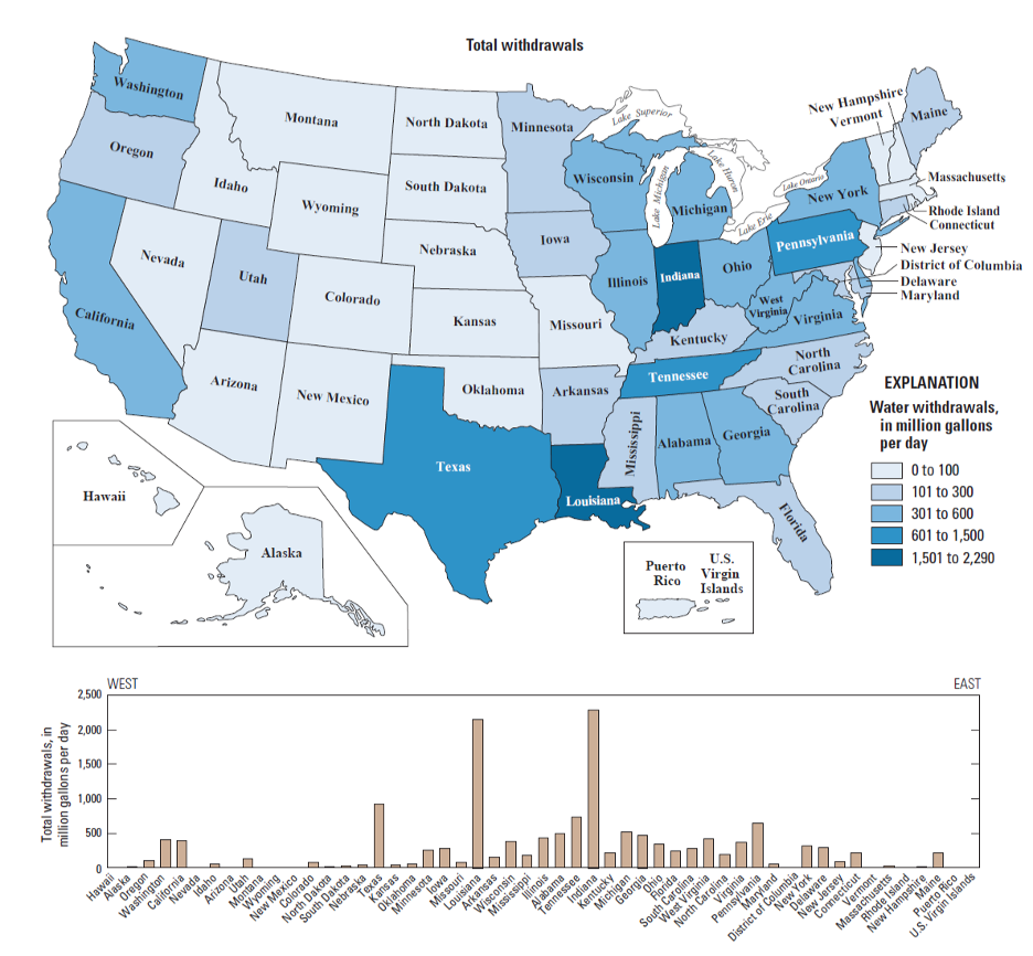
| State | Water Withdraws million gal/day |
|---|---|
| Hawaii | 100 |
| Alaska | 100 |
| Oregon | 250 |
| Washington | 500 |
| California | 200 |
| Nevada | 100 |
| Idaho | 100 |
| Arizona | 100 |
| Utah | 250 |
| Montana | 100 |
| Wyoming | 100 |
| New Mexico | 100 |
| Colorado | 200 |
| North Dakota | 100 |
| South Dakota | 100 |
| Nebraska | 100 |
| Texas | 2200 |
| Kansas | 100 |
| Oklahoma | 100 |
| Minnesota | 200 |
| Iowa | 300 |
| Missouri | 100 |
| Louisiana | 3200 |
| Arkansas | 250 |
| Wisconsin | 500 |
| Mississippi | 300 |
| Illinois | 400 |
| Alabama | 500 |
| Tennessee | 800 |
| Indiana | 2400 |
| Kentucky | 250 |
| Michigan | 700 |
| Georgia | 600 |
| Ohio | 650 |
| Florida | 250 |
| South Carolina | 300 |
| West Virginia | 1100 |
| North Carolina | 300 |
| Virginia | 500 |
| Pennsylvania | 900 |
| Maryland | 250 |
| D.C. | 100 |
| New York | 300 |
| Delaware | 100 |
| New Jersey | 100 |
| Connecticut | 200 |
| Vermont | 100 |
| Massachusetts | 200 |
| Rhode Island | 100 |
| New Hampshire | 100 |
| Maine | 250 |
| Puerto Rico/US Virgin Islands | 100 |
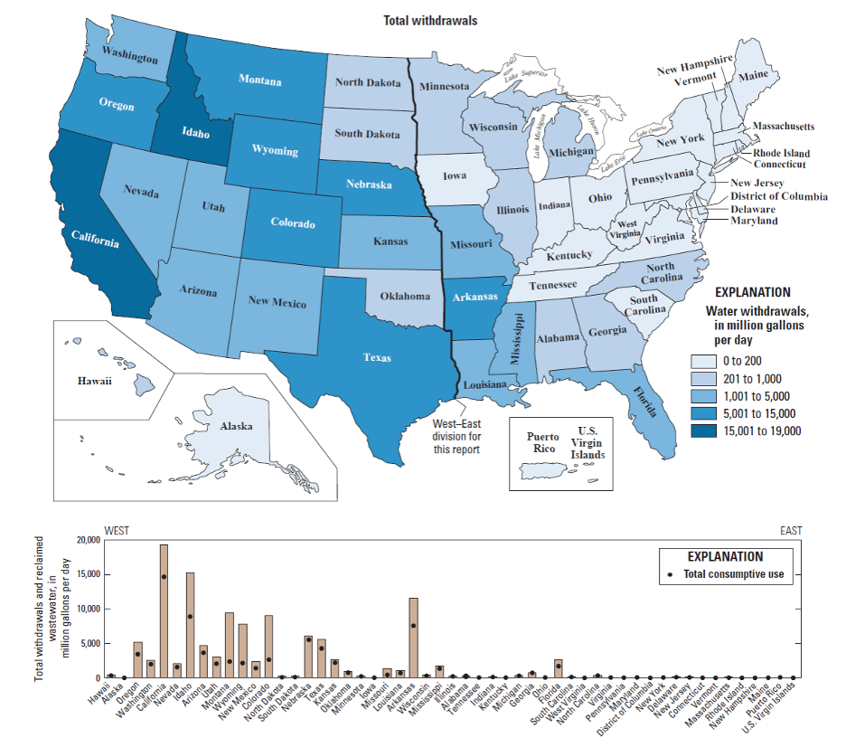
| State | Water Withdraws million gal/day |
|---|---|
| Hawaii | 200 |
| Alaska | 200 |
| Oregon | 6000 |
| Washington | 3000 |
| California | 24000 |
| Nevada | 1500 |
| Idaho | 16000 |
| Arizona | 5000 |
| Utah | 4000 |
| Montana | 10000 |
| Wyoming | 4000 |
| New Mexico | 2000 |
| Colorado | 13000 |
| North Dakota | 200 |
| South Dakota | 200 |
| Nebraska | 9000 |
| Texas | 8500 |
| Kansas | 2000 |
| Oklahoma | 500 |
| Minnesota | 300 |
| Iowa | 200 |
| Missouri | 1500 |
| Louisiana | 900 |
| Arkansas | 9000 |
| Wisconsin | 300 |
| Mississippi | 2000 |
| Illinois | 500 |
| Alabama | 200 |
| Tennessee | 200 |
| Indiana | 200 |
| Kentucky | 200 |
| Michigan | 300 |
| Georgia | 750 |
| Ohio | 200 |
| Florida | 3500 |
| South Carolina | 200 |
| West Virginia | 200 |
| North Carolina | 200 |
| Virginia | 200 |
| Pennsylvania | 200 |
| Maryland | 200 |
| D.C. | 200 |
| New York | 200 |
| Delaware | 200 |
| New Jersey | 200 |
| Connecticut | 200 |
| Vermont | 200 |
| Massachusetts | 200 |
| Rhode Island | 200 |
| New Hampshire | 200 |
| Maine | 200 |
| Puerto Rico/US Virgin Islands | 200 |
The source of the water we use also provides clues about where water may be most readily available, and/or where typical rainfall and snowmelt cannot meet demand. Inspect the maps below (Figure 16). Surface water withdrawals are spread more or less uniformly across the U.S., and reflect overall water use reasonably closely. This is influenced in large part by total population, energy production, and industrial and agricultural activity (i.e. CA, TX, NY, and FL are the most populous states). However, groundwater withdrawals (obtained by pumping at wells) are a good indication that surface water flows alone are not sufficient to meet demand.
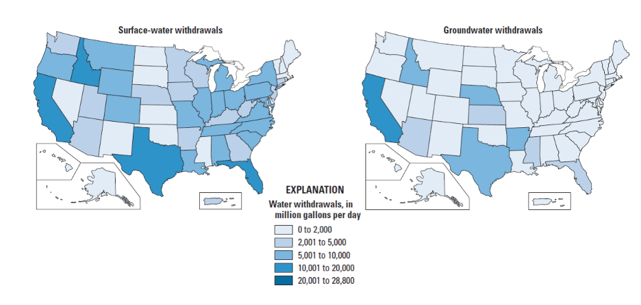
| Amount (million gals./day) | States (random order) |
|---|---|
| 1500-3200 | CA |
| 600-1500 | ID, TX, CO, IL, MI, OH, NY, NC, VA, TN, |
| 300-600 | OR, MO, WI, IN, PA, NJ, DE, SC, AL, LA, AK |
| 300 | All others |
| Amount (million gals./day) | States (random order) |
|---|---|
| 1500-3200 | n/a |
| 600-1500 | CA |
| 300-600 | TX, NE, AK |
| <300 | All others |
Demand for Water
Demand for Water
As shown in the Freshwater Resources section, water demand varies by culture and country, while water availability is dependent on climate and geography (see also Module 2). Some areas of the world are already experiencing freshwater shortages and/or their water supplies are unsanitary as the result of improper treatment of waste and inadequate infrastructure to transport and store potable water. The combined specters of climate change and rapid population growth create uncertainty in planning future water supplies.
Future Demand for Water
Future Demand for Water
What will the future bring?
What will the future bring? Good question, right? How can we gauge what water demand and availability will be in the future, particularly with projected large increases in population and potential climate change superimposed? Not to alarm you, but to inform you, we will go through the exercise of making such projections, both for the U.S. and, on a more limited basis, for the world. What do we need to know for making such estimates? First, let's jot down some ideas. Then we will continue the process below.
Food for Thought
1. What do you think we would need to know in order to predict future demand for water? Take a minute to jot down what you think one would need to take the first crack at this.
ANSWER: Answers will vary. Clearly, we will need to know something about population growth and climate.
First, here is an expert opinion as to how the future will go…
In Human Population and the Environmental Crisis Ben Zuckerman and David Jefferson write: “At a low population density, a society may be able to derive its water from rivers, natural lakes, or from the sustainable use of groundwater. As the population grows, so does the volume of water needed (we will assume demand is proportional to population size). Moreover, levels of waste discharge into the environment will grow as the population rises. Thus, the available unmanaged supplies deteriorate at the same time that demand on them is increasing…A destructive synergy is at work: population size affects the water resource in a manner that is not one of simple proportionality.”
What was it Yogi Berra (N.Y. Yankees catcher and later Manager) infamously said…"It's tough to make predictions, especially about the future." Well, that is a truism, but let's see what projections are being made regarding future population growth, because, clearly, that's one of the inputs we need to determine potential future water use globally.The present global population (as of 2024) is approximately 8.05 billion people. Interestingly, the top three countries, in terms of population, are China, India, and, yes, the United States, in that order (Figure 17). But, by 2050 the global population is estimated to be 9.7 billion people by the United Nations—a staggering 20% increase in the next, say, 26 years! So, at the minimum, if we assume that water use will increase linearly on a per person basis, we would expect that this rate of growth will require 20% more fresh water by 2050. Is that a problem? Do we have excess capacity to supply this water?
Population Growth vs. Water Needs
Population Growth vs. Water Needs
Do we have excess capacity to supply this water? That is an important question, but you have probably already determined that the real issue is where the population growth occurs and what water resources are available there. The major growth is projected to occur in developing countries (Figure 17). African nations are likely regions for greater than average growth. Interestingly, much of Africa is estimated to have significant groundwater resources (BGS, 2013) that could be developed if necessary. In fact, Nigeria is projected to surpass the population of the U.S. by 2050 (Figures 17-19). One must examine the population density and rate of projected growth vs. water needs. In addition, climate change impacts must be considered.


1950- total population 2.5 bn
- China- .5 billion
- India
- United States
- Russia
- Japan
- Indonesia
- Germany
- Brazil
- Britain
- Italy
2013- total population 7.2 bn
- China-4 bn
- India
- United States
- Indonesia
- Brazil
- Pakistan
- Nigeria
- Bangladesh
- Russia
- Japan
2050 forecast- total population 9.6 bn
- India-7 bn
- China
- Nigeria
- United States
- Indonesia
- Pakistan
- Brazil
- Bangladesh
- Ethiopia
- Philippines

Learning Checkpoint
1. What is the relationship between Total Fertility and Per Capita Income shown in Figure 19 above?
ANSWER: Fertility is inversely related to income worldwide. There are several drivers of this relationship, including infant mortality, need for agrarian labor, etc.
2. Why might this be an important consideration when considering future demand for water?
ANSWER: The greatest growth is likely to occur in areas with the least access to infrastructure for accessing, treating, and distributing fresh water.
Increased Impacts of Climate Change on Demand
Increased Impacts of Climate Change on Demand
We would probably be better off examining the impacts of climate change on water availability that would increase "water stress," then compare these stresses with those caused by increasing demand, either by population growth in a given region (personal or agricultural demands) or increased water usage resulting from new demands (e.g., energy production) (Figure 20). A number of studies have predicted water supply vs. water demand relationships resulting from climate change. A study by MIT (Massachusetts Institute of Technology) researchers (Schlosser et al., 2014) compared the potential impacts of climate change, on the basis of projected greenhouse gas emission increases in a complex Earth-system model, on water stress in 282 assessment regions (large or multiple watersheds) globally, holding demand constant, to the potential impacts of population growth in the same regions.


| Country | Increase/Decrease | Percent |
|---|---|---|
| US | Increase | 28 |
| Mexico | Increase | 32 |
| Brazil | Increase | 18 |
| Germany | Decrease | 13 |
| Nigeria | Increase | 176 |
| Kenya | Increase | 138 |
| India | Increase | 34 |
| China | Increase | 2 |
| Japan | Decrease | 15 |
| Russia | Decrease | 16 |
They found that, in most regions, projected population growth with increased demand to 2050 was the greater stressor. These researchers use a Water Stress Index (WSI) defined as WSI = TWR/RUN+INF (TWR is total water required for a given watershed region, i.e. all consumptive uses, RUN is available runoff within the watershed, and INF is inflow to the watershed from adjacent regions. The cutoffs used for interpreting water stress are: WSI<0.3 is slightly exploited, 0.3≤WSI<0.6 moderately exploited, 0.6≤WSI<1 heavily exploited, 1≤WSI<2 overly exploited, and WSI≥2 extremely exploited as originally set out by Smakhtin et al. (2005).
It appears that a substantial proportion of Africa, all of the middle East, India, and central Asia will see increased water stress in the next few decades, largely due to projected population increases. Even the southwestern U.S. is projected to experience expansion and intensification of water stress, but, in this case, mostly as the result of climate change and longer-term drought. Interestingly, the major central U.S. groundwater source, the Ogallala Aquifer, does not appear to be a candidate for significant stress except at its southern end in Texas. However, other studies (see Module 7) suggest that depletion of this aquifer will be more severe.
Possible Solutions for Meeting Water Demand in Stressed Regions
Possible Solutions for Meeting Water Demand in Stressed Regions
There are a number of possible methods to enhance supplies of fresh water, each of which has an economic, political, and/or environmental impact.
Learning Checkpoint
1. Provide three examples of potential ways to increase fresh water supplies.
ANSWER: Answers may vary. There are a number of potential strategies, including 1) Build large dams to increase water storage; 2) Bank water in groundwater storage; 3) Encourage transfers from other consumptive uses and/or conservation; 4) Increase recycling and reuse of wastewater; 5) Desalination of seawater or shallow saline groundwater.
Some of these strategies have been alluded to previously (e.g., encouraging transfers from agricultural use to drinking water supplies). Water storage behind dams is an old strategy and problematic in a number of ways (see Module 6), including high costs, environmental impacts, and political issues that arise when major rivers flow through multiple countries. Nonetheless, there is still major proposed and ongoing dam building in China and other countries.
Groundwater banking is a newer strategy that requires replenishment of aquifers with treated wastewater and/or with runoff available during times of excess. Costs are associated with treating, impounding, and injecting the water (see Module 7). This will mainly benefit regions with significant groundwater resources.
Recycling and reuse are gaining support with successful projects in the U.S. and elsewhere. Penn State University recycles and reinjects nearly 98% of its treated wastewater and has done so since the 1960s. Orange County, CA, has another successful system (see Module 8). Such systems must overcome consumer opposition, however, because of the perception that consumers will be drinking, well, toilet water! Nonetheless, the water quality in such systems is as good or better than that in municipalities that draw water from rivers downstream from other municipalities that discharge treated wastewater into the same river. Another form of reuse is to employ "gray" water (only partially treated) for irrigation of golf courses in arid to semiarid, water-stressed regions. Las Vegas, NV, has implemented such a system, coupled with the removal of water-hungry turf, for which the economics work and conservation is encouraged.
Desalination may be a last resort because of the costs of energy required to remove salts from seawater or water pumped from saline aquifers in non-coastal regions. However, in water-poor but hydrocarbon-rich middle-Eastern countries the economics may support the desalination of seawater. Alternative energy sources (e.g., solar) or emerging processes such as chemical reverse osmosis may be economical in the future as they become more efficient and less costly. And, of course, if water is deemed to have significant value in the future, the high costs may be more acceptable.
Finally, there are still proposals to import or export water from regions replete with fresh water resources (e.g. Alaska) to severely water-stressed regions (e.g. India). However, the costs of transporting such a commodity across the oceans would appear to exceed the value of that water at its terminus.
All of these strategies will be explored in later modules in more detail.
Pricing Water
Pricing Water

Does water have value? If so, how do we set a price for it? And, if we agree that individual access to fresh water is a basic human right or expectation globally (is this generally agreed?), how do we treat water as a commodity? Do we really pay what water is worth?
Pricing Varies
Pricing Varies
You are likely all too familiar with bottled water—that convenient liter-sized plastic bottle containing some sort of water, commonly tap water, or filtered spring water, sometimes treated…it appears that, in the U.S., we pay for the convenience of "grab-and-go." For that convenience, we typically pay about $4/gallon, more than we presently pay for a gallon of gasoline! In most municipalities; however, the cost of water delivered in pipes to taps in homes costs far less ($0.003-0.006/gallon). survey by CircleofBlue.org for 2019 water pricing in 30 cities across the U.S. found an average increase of 3.2% in monthly bills for a family of four using an average of 100 gals/day each (12,000 gals/mo or 45.4 m3/mo) from 2018 to 2019, costing an average of $72.93 a month.
Monthly rates for some representative municipalities are shown in the table below, based on data in the CircleofBlue.org 2014 survey and information from water authority websites for some municipalities not covered in that survey (Pittsburgh, PA and State College, PA).Note the large range in rates that do not seem to make sense geographically. For example, arid Phoenix, AZ has the lowest rate, with Las Vegas, NV not far behind, whereas high precipitation, seemingly water-rich regions such as Seattle, WA and Atlanta, GA top the rate list. Note that Los Angeles, CA, Phoenix, AZ, and Las Vegas, NV all depend on Colorado River water, although Los Angeles also draws on northern California sources and all require significant transport infrastructure. So, in part, this disparity in rates results from the costs of maintaining infrastructure and the numbers of households served, as well as the local abundance of water.
| Municipality (city, state) | Monthly rate (12,000 gals) | Percentage change (2014-2013) |
|---|---|---|
| Phoenix, AZ | $38.75 | 0 |
| Chicago, IL | $39.72 | +14.9 |
| Las Vegas, NV | $42.27 | +2.8 |
| State College, PA | $47.40 | 0 |
| New York, NY | $57.28 | +5.6 |
| Philadelphia, PA | $65.88 | +5.0 |
| Los Angeles, CA | $75.98 | +14.5 |
| Atlanta, GA | $91.92 | 0 |
| Seattle, WA | $98.77 | +9.3 |
| Pittsburgh, PA | $100.81 | ? |
Chicago, IL, for example, has nearby Lake Michigan as a source and a large number of users and its rates are relatively low. Little State College, PA has a significant, sustainable groundwater resource (see Module 6), even though the user base is relatively small. Many municipalities have higher rates because they are financing necessary improvements in infrastructure, which can be quite costly.
Municipalities have adopted different methods for scaling water prices. Some, such as Philadelphia and Detroit, provide cost reductions for larger users (decreasing block), some, including New York, have uniform pricing, whereas others, such as Las Vegas and Atlanta, have implemented tiered pricing (block increases) that encourage conservation while trying to maintain the user base. The objective of all municipalities is to sustain income and provide for future infrastructure requirements.
Internationally, pricing varies even more than in the U.S. Figure 22 illustrates average water prices (Kariuki and Schwartz, 2005) and the impact of non-public water suppliers on the cost to the consumer. Where public utilities are not available, the cost to the consumer can be a factor of 10 higher. In part, this occurs because of increases in cost to the water supplier to purchase water from a public or private supplier because of the large volumes purchased with prevailing block pricing increases. Figure 23 shows the step increases for several African and Indian cities. Recall that the average family of four in the U.S. would use about 45 m3/month, but average usage is probably much lower in many developing nations with lower standards of living. Step increases in block pricing appear to be a fair method of pricing to allow low cost for low-volume users and encouraging conservation by imposing higher costs for larger-volume users.


The Water and Energy Nexus
The Water and Energy Nexus
Considerations of water pricing are complicated because of the multitude of factors that must be taken into account. These include availability and dependability of water supply locally, state of the distribution infrastructure, and the distribution and size of the user base. Dependability is related to climate impacts, such as prolonged droughts that deplete water reserves. A recent study (Watergy Nexus: The Complex Relationship and Looming Crisis Between Our Thirst For Water and Our Hunger for Energy [18]) highlights an additional factor—the amount and cost of energy to acquire, transport, and treat water. This study argues that the cost of energy (usually electricity, but including fuel if the water is trucked in) must be considered in pricing water. The study uses data for 2013, a year of severe drought in much of the western and central U.S. to show how water prices should be adjusted to guarantee supply and cover costs of acquisition. Although the U.S. Geological Survey indicates that the average energy required to provide 1000 gallons (1 kgal) of water is 1.9kWh of electricity, water-stressed regions such as northern California (3.5 kWh/kgal) and highly stressed southern California (11.1 kWh/kgal) require far more (Figure 24). However, the study suggests that municipalities are not taking this factor into consideration in providing a durable and resilient water supply. During times of water stress, municipalities may have trouble meeting costs, and begin to examine other strategies, such as privatization. Of course, when water availability becomes restricted, costs can go up as in California with severe drought conditions (e.g., see the news article In dry California, water fetching record prices [19] about California water pricing: ).

Learning Checkpoint
1. What factors drive water pricing?
ANSWER: Factors that must be considered include: the availability and dependability of water supply locally, state of the distribution infrastructure and potential costs needed to improve or maintain it, cost of delivery – including energy, distribution, and size of the user base, and demand.
Privatization
Privatization
Cash-strapped municipalities with failing water systems might be tempted to contract with private companies to manage their water and sewer systems. Economic drivers, such as the collapse that occurred in 2008, affect users ability to pay for public water systems. In the U.S., about 20% of water supplies are privatized at present. In evaluating this option, one must keep in mind that corporations are for-profit entities, and will need to recoup the full costs of providing water while adding a margin for profit to benefit the corporation and/or their stockholders. Public utilities can be held responsible for controlling costs and providing clean water supplies, whereas it is more difficult for the public to do so for private companies.
There are a number of examples where privatization has apparently failed consumers. Pushed by the costs of renovating their failing water supply infrastructure, Atlanta, GA, for example, handed over control of their water system to United Water, which took over in 1999, with a 20-year contract. Atlanta had long-deferred most maintenance because their revenue was insufficient to cover the full cost of providing service, and because of rapid population growth and their aging system, expansion and improvement were required. Their sewage system was more of a problem than the water supply system, and they were being sued under the U.S. Clean Water Act for that problem as well.
But, in 2003, the city of Atlanta withdrew from the agreement because a number of issues with United Water (see What Can We Learn From Atlanta's Water Privatization [21] for the full story), which included costs, viewed as excessive, and poor performance in maintenance, meter installation, and bill collection.
The situation in Detroit has been much in the news of late (for example – see this MSNBC article, Detroit residents and national allies protest water shutoffs [22]). As a result of the economic downturn, the Detroit Water and Sewer Department has recently gone on a campaign to force users to pay their outstanding water bills with the threat of cutoffs. In addition, the city of Detroit is pursuing the possibility of privatizing its water and sewer systems. Although clearly having its own perspective and position, an interesting argument against water privatization in Detroit [23] is found on The Blue Planet Project website. One common argument against privatization is the rapid increase in the costs of water to consumers. Of course, in many cases, this may occur because the public purveyor was not charging for the full cost of providing the water in the first place.
Michigan lawmakers propose that water bills are capped at 3% of households income and $2 added to bills that can afford to make up for lost income. Claiming that shutting off water is a human rights violation. Read more here. [24]
A 2022 Cornell Chronical story explains that private ownership had the largest impact on annual water bills, which averaged $144 higher in privately owned systems than in public sector systems. Low-income households served by private operators spent 4.4% of their income on water service, about 1.5 percentage points more than in communities with public ownership.
Module 2: Climatology of Water
Module 2: Climatology of Water
Overview
In this module, we will investigate the underlying causes of variations in precipitation on Earth, with a specific focus on large-scale climate belts and the role of mountain ranges in affecting the distribution of rainfall (and snow). The goals of the module are to develop a quantitative understanding of the physical processes that control the distribution of precipitation, and which ultimately govern regions where water is abundant and where it is scarce, both across the U.S. and globally. As part of this, you’ll develop facility with the concepts of relative humidity, saturation, water vapor content in the air, and how these vary with changes in temperature - all of which play a key role in determining when and where precipitation falls.
Goals and Learning Objectives
Goals and Learning Objectives
Goals
- Explain the distribution and dynamics of water at the surface and in the subsurface of the Earth
- Interpret graphical representations of scientific data
Learning Objectives
In completing this module, you will:
- Identify the unique physical properties of water that contribute to its fundamental role in driving Earth Systems
- Identify U.S. and global precipitation patterns by reading precipitation maps
- Quantitatively compare fluxes of water in the hydrologic cycle
- Calculate relative humidity, and use it to quantitatively explain Earth's first-order patterns of precipitation
- Assess the relationship between precipitation, topography, and location on the globe
Unique Properties of Water
Unique Properties of Water
Water has some unusual properties that most of us do not really appreciate or understand. These properties are crucial to life and they originate from the structure of the water molecule itself. This sidebar will provide an overview of water's properties that will be useful in understanding the behavior of water in Earth's environment.
The Configuration of the Water Molecule
The Configuration of the Water Molecule
A molecule of water is composed of two atoms of hydrogen and one atom of oxygen. The one and only electron ring around the nucleus of each hydrogen atom has only one electron. The negative charge of the electron is balanced by the positive charge of one proton in the hydrogen nucleus. The electron ring of hydrogen would actually prefer to possess two electrons to create a stable configuration. Oxygen, on the other hand, has two electron rings with an inner ring having 2 electrons, which is cool because that is a stable configuration. The outer ring, on the other hand, has 6 electrons but it would like to have 2 more because, in the second electron ring, 8 electrons is the stable configuration. To balance the negative charge of 8 (2+6) electrons, the oxygen nucleus has 8 protons. Hydrogen and oxygen would like to have stable electron configurations but do not as individual atoms. They can get out of this predicament if they agree to share electrons (a sort of an energy "treaty"). So, oxygen shares one of its outer electrons with each of two hydrogen atoms, and each of the two hydrogen atoms shares it's one and only electron with oxygen. This is called a covalent bond. Each hydrogen atom thinks it has two electrons, and the oxygen atom thinks that it has 8 outer electrons. Everybody's happy, no?
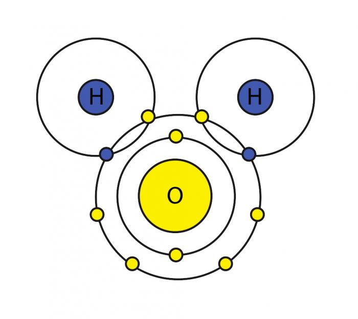
However, the two hydrogen atoms are both on the same side of the oxygen atom so that the positively charged nuclei of the hydrogen atoms are left exposed, so to speak, leaving that end of the water molecule with a weak positive charge. Meanwhile, on the other side of the molecule, the excess electrons of the oxygen atom, give that end of the molecule a weak negative change. For this reason, a water molecule is called a "dipolar" molecule. Water is an example of a polar solvent (one of the best), capable of dissolving most other compounds because of the water molecule's unequal distribution of charge. In solution, the weak positively charged side of one water molecule will be attracted to the weak negatively charged side of another water molecule and the two molecules will be held together by what is called a weak hydrogen bond. At the temperature range of seawater, the weak hydrogen bonds are constantly being broken and re-formed. This gives water some structure but allows the molecules to slide over each other easily, making it a liquid.
The Structure of Water: Properties
The Structure of Water: Properties
Studies have shown that clustering of water molecules occurs in solutions because of so-called hydrogen bonds (weak interaction), which are about 10% of the covalent water bond strength. This is not inconsiderable and energy is required to break the bonds, or is yielded by the formation of hydrogen bonds. Such bonds are not permanent and there is constant breaking and reforming of bonds, which are estimated to last a few trillionths of a second. Nonetheless, a high proportion of water molecules are bonded at any instant in a solution. But this structure leads to the other important properties of water.
We will consider, for the purposes of this course, only six of these important properties:
- Heat capacity
- Latent heat (of fusion and evaporation)
- Thermal expansion and density
- Surface Tension
- Freezing and Boiling Points
- Solvent properties
As mentioned above, these properties have importance to physical and biological processes on Earth. Effectively, large amounts of water buffer Earth surface environmental changes, meaning that changes in Earth-surface temperature, for example, are relatively minor. Thus, the high heat capacity of water promotes continuity of life on Earth because water cools/ warms slowly relative to land, aiding in heat retention and transport, minimizing extremes in temperature, and helping to maintain uniform body temperatures in organisms. However, there are other effects of water properties as well. Its low viscosity allows rapid flow to equalize pressure differences. Its high surface tension allows wind energy transmission to sea surface promoting downward mixing of oxygen in large water bodies such as the ocean. In addition, this high surface tension helps individual cells in organisms hold their shape and controls drop behavior (have you seen "An Ant's Life"?). Also, the high latent heat of evaporation is very important in heat/water transfer within the atmosphere and is a significant component of transfer of heat from low latitudes, where solar energy influx is more intense to high latitudes that experience solar energy deficits.
Video: Water - Liquid Awesome: Crash Course Biology #2 (11:16)
Take a few minutes to learn why water is the most fascinating and important substance in the universe.
Ah, hello there, here at crash course HQ we like to start out each day with a nice healthy dose of water in all its three forms it is the only substance on all of our planet Earth that occurs naturally in solid liquid and gas forms and to celebrate this magical bond between two hydrogen atoms and one oxygen atom here today we are going to be celebrating the wonderful life-sustaining properties of water but we're going to do it slightly more clothed. Much better.
We left off here at the biology crash course we're talking about life and the rather important fact that all life as we know it is dependent upon there being water around I'm just an astronomers are always looking out into the universe trying to figure out whether there is life elsewhere because you know that is kind of the most important question that we have right now I was getting really excited when they find water someplace particularly liquid water, and this is one reason why I and so many other people geeked out so hard last December when on Mars a seven-year-old rover Opportunity found a 20 inch long vein of gypsum that was almost certainly deposited by like long-term liquid water on the surface of Mars and this was probably billions of years ago. And so it's going to be hard to tell whether or not the water that was there resulted in some life, but maybe we can figure that out and that would be really exciting. But why do we think that water is necessary for life? Why does water on other planets get us so friggin excited?
So let's start out by investigating some of the amazing properties of water. In order to do that we're gonna have to start out with this the world's most popular molecule or at least the world's most memorized molecule, we all know about it good old h2o. Two hydrogens one oxygen the hydrogen's each sharing an electron with oxygen in what we call a covalent bond. So as you can see you have drawn my water molecule in a particular way and this is actually the way that it appears it is v-shaped because this big ol oxygen atom is a little bit more greedy for electrons. It has a slight negative charge whereas this area here with the hydrogen atoms has a slight positive charge thanks to this polarity all water molecules are attracted to one another so much so that they actually stick together and these are called hydrogen bonds and we talked about the last time essentially what happens is that the positive pole around those hydrogen atoms bonds to the negative pole around the oxygen atoms of a different water molecule and so it's a weak bond but look they're bonding seriously I cannot overstate the importance of this hydrogen bond so when your teacher asks you what's important about water start out with hydrogen bonds and you should put it in all gaps and maybe some sparkles around it one of the cool properties that results from these hydrogen bonds is a high cohesion for water which results in high surface tension cohesion is the attraction between - like things like attraction between one molecule of water and another molecule of water water has the highest cohesion of any nonmetallic liquid and you can see this if you put some water on some wax paper or some Teflon or something where the water beads up like that some some leaves of plants do it really well. It's quite cool since water adheres weakly to the wax paper or to the plant but strongly to itself the water molecules are holding those droplets together in a configuration that creates the least amount of surface area it's this high surface tension that allows some bugs and even I think one lizard and also one Jesus to be able to walk on what a Cui's of force of water does its limits.
Of course, there are other substances that water quite likes to stick to. Take glass for example, this is called adhesion and the water is spreading out here instead of beating up because the adhesive forces between the water and the glass are stronger than the cohesive forces of the individual water molecules in the bead of water adhesion is attraction between two different substances so in this case the water molecules and glass molecules these properties lead to one of my favorite things about water is the fact that it can defy gravity. That really cool thing that just happened is called capillary action and explaining it can be easily done with what we now know about cohesion and adhesion thanks to adhesion the water molecules are attracted to the molecules in the straw but as the water molecules adhere to the straw other molecules are drawn in by cohesion following those fellow water molecules thank you cohesion the surface tension created here causes the water to climb up the straw and it will continue to climb until eventually gravity pulling down on the weight of the water and the straw overpowers the surface tension. The fact that water is a polar molecule also makes it really good at dissolving things.
It's a good solvent, scratch that water isn't a good solvent, it's an amazing solvent! There are more substances that can be dissolved in water than in any other liquid on earth and yes that includes the strongest acid that we have ever created these substances that dissolve in water is sugar or salt being ones that we're familiar with are called hydrophilic and they are hydrophilic because they are polar and their polarity is stronger than the cohesive forces of the wall, so when you get one of these polar substances in water it's strong enough that it breaks all the little cohesive forces. All those little hydrogen bonds and instead of hydrogen bonding to each other the water will hydrogen bond around these polar substances table salt is ionic and right now it's being separated into ions as the poles of our water molecules interact with it but what happens when there is a molecule that cannot break the cohesive forces of water it can't penetrate and come into it basically what happens when that substance can't overcome the strong cohesive forces of water and can't get inside of the water? That's what we get what we call hydrophobic substance or if something that is fearful of water.
These molecules lacked charged poles they are nonpolar and are not dissolving in water because essentially they're being pushed out of the water by water's cohesive forces water we may call it the universal solvent but that does not mean that it dissolves everything there have been a lot of eccentric scientists throughout history but all this talk about water got me thinking about perhaps the most eccentric of the eccentrics a man named Henry Cavendish he communicated with his female servants only via notes and added a staircase to the back of his house to avoid contact with his housekeeper. Some believe he may have suffered from a form of autism but just about everyone will admit that he was a scientific genius. He's best remembered as the first person to recognize hydrogen gas as a distinct substance and to determine the composition of water in the 1700s most people thought that water itself was an element but Cavendish observed that hydrogen which he called inflammable air reacted with oxygen known then by the awesome name defroster gated air to form water. Cavendish didn't totally understand what he'd discovered here in part because he didn't believe in chemical compounds he explained his experiments with hydrogen in terms of a fire like element called phlogiston nevertheless his experiments were groundbreaking like his work and determining the specific gravity basically the comparative density of hydrogen and other gases with reference to common air it's especially impressive when you consider the crude instruments he was working with this for example is what he made his hydrogen gas with he went on not only to establish an accurate composition of the atmosphere but also discovered the density of the earth not bad for a guy who was so painfully shy that the only existing portrait of him was sketched without his knowledge so for all of his decades of experiments only published about 20 papers in the years after his death researchers figured out that Cavendish had actually pre discovered Richter's law Ohm's law Coulomb's law several other laws that's a lot of freakin laws and if he had gotten credit for them all we would have had to deal with like Cavendish's eight flaw and Cavendish's fourth law. So I for one am glad that he didn't actually get credit.
We're gonna do some pretty amazing science right now you guys are not going to believe this okay you ready, it floats. Yeah I know you're not surprised by this but you should be because everything else when it's solid is much more dense than when it's liquid just like gases are much less dense than liquids are but that simple characteristic of water that it's solid form floats is one of the reasons why life on this planet as we know it is possible and why is it that solid water is less dense than liquid water while everything else is the exact opposite of that. Well you can thank your hydrogen bonds once again so at around 32 degrees Fahrenheit or zero degrees Celsius if you're a scientist or from a part of the world where things make sense water molecules start to solidify and the hydrogen bonds in those water molecules form crystalline structures that space molecules apart more evenly in turn making frozen water less dense than its liquid form so in almost every circumstance of floating water ice is a really good thing if I swear denser than water it would freeze and then sink and then freezing than sinking than freezing than sink so just trust me on this one you don't want to live on a world where I sinks not only would it totally wreak havoc on aquatic ecosystems which are basically how life formed on the earth in the first place it would also you know all the ice and the North Pole would sink and then all of the water everywhere else would rise and we wouldn't have any land that would be annoying.
There's one more amazing property of water that I'm forgetting so why is it so hot in here. Oh heat capacity yes water has a very high heat capacity and probably that means nothing to you but basically it means that water is really good at holding on to heat which is why we like to put hot water bottles in our bed and with them when we're lonely but aside from artificially warming your bed it's also very important that it's hard to heat up and cool down the oceans significantly they become giant heat sinks that regulate the temperature and the climate of our planet which is why for example it's so much nicer in Los Angeles where the ocean is constantly keeping the temperatures the same then it is and say Nebraska on a smaller scale we can see waters high heat capacity really easily and visually by putting a pot with no water in it on a stove and seeing how badly that goes but then you put a little bit of water in it and it takes forever to frickin boil oh and if you haven't already noticed this or when water evaporates from your skin it cools you down now that's the principle behind sweating which is an extremely effective though somewhat embarrassing part of life but this is an example of another incredibly cool thing about water when my body gets hot and it sweats that heat excites some of the water molecules on my skin to the point where they break those hydrogen bonds and they evaporate away and when they escape they take that heat energy with them leaving me cooler lovely well this wasn't exercise though I don't know why sweating so much it could be the spray bottle that I keep spraying myself with her maybe it's just because this is such a high-stress enterprise trying to teach you people things I think I need some water but while I'm drinking ah there's review for all of the things that we talked about today if you there are a couple things that you're not quite sure about just go back and watch them it's not going to take a lot of your time and you're going to be smarter. I promise you're going to do so well on that test you either don't or do have coming up okay bye
Heat Capacity
Heat Capacity
Water does not give up or take up heat very easily. Therefore, it is said to have a high heat capacity. In Colorado, it is common to have a difference of 20˚ C between day and night temperatures. At the same time, the temperature of a lake would hardly change at all. This property originates because energy is absorbed by water as molecules are broken apart or is released by molecules of water associating as clusters.
Video: Heat Capacity of Water (01:13)
Take a few minutes to watch the video below to help you understand heat capacity.
The video begins by showing two candles and two balloons. One balloon (the yellow one) is partially filled with water. Both candles are lit and the ballons are moved so they are directly on top of the flame. The balloon without water bursts. This happens because the water absorbs the heat from the flame. The balloon is then picked up to reveal that the bottom of the balloon is burnt.
Latent Heat and Freezing and Boiling Points
Latent Heat and Freezing and Boiling Points
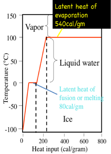
A calorie is the amount of heat it takes to raise the temperature of 1 gram (0.001 liters) of pure water 1 degree C at sea level. It takes 100 calories to heat 1 g. water from 0˚, the freezing point of water, to 100˚ C, the boiling point. However, 540 calories of energy are required to convert that 1 g of water at 100˚ C to 1 g of water vapor at 100˚ C. This is called the latent heat of vaporization. On the other hand, you would have to remove 80 calories from 1 g of pure water at the freezing point, 0˚ C, to convert it to 1 g of ice at 0˚ C. This is called the latent heat of fusion.
Interestingly, the latent heat and freezing and boiling points are controlled by the way water molecules interact with one another. Because molecules acquire more energy as they warm, the association of water molecules as clusters begins to break up as heat is added. In other words, the energy is absorbed by the fluid and molecules begin to dissociate from one another. Considerable energy is required to break up the water molecule clusters, thus there is relatively little temperature change of the fluid for a given amount of heating (this is the heat capacity measure), and, even at the boiling point, it takes far more energy to liberate water molecules as a vapor (parting them from one another). On the other hand, when energy is removed from water during cooling the molecules of water begin to coalesce into clusters and this process adds energy to the mix, thus offsetting the cooling somewhat.
Click here for a text description
Thermal Expansion and Density
Thermal Expansion and Density
When water is a liquid, the water molecules are packed relatively close together but can slide past each other and move around freely (as stated earlier, that makes it a liquid). Pure water has a density of 1.000 g/cm3 at 4˚ C. As the temperature increases or decreases from 4˚ C, the density of water decreases. In fact, if you measure the temperature of the deep water in large, temperate-latitude (e.g., the latitude of PA and NY) lakes that freeze over in the winter (such as the Great Lakes), you will find that the temperature is 4˚ C; that is because fresh water is at its maximum density at that temperature, and as surface waters cool off in the Fall and early Winter, the lakes overturn and fill up with 4˚ C water.

However, as dissolved solids are added to pure water to increase the salinity, the density increases. The density of average seawater with a salinity of 35 o/oo (35 g/kg) and at 4˚ C is 1.028 g/cm3 as compared to 1.000g/cm3 for pure water. As you add salts to seawater, you also change some other properties. Incidentally, increasing salinity increases the boiling point and decreases the freezing point. Normal seawater freezes at -2˚ C, 2˚ C colder than pure water. Increasing salinity also lowers the temperature of maximum density. This effect also helps explain why you are supposed to add salt to ice when making ice cream or to add salt to water when cooking spaghetti (although, in this case, the effect on boiling point is minor and the added salt is mainly for flavor).
When water freezes, however, bonds are formed that lock the molecules in place in a regular (hexagonal) pattern. For nearly every known chemical compound, the molecules are held closer together (bonded) in the solid state (e.g., in mineral form or ice) than in the liquid state. Water, however, is unique in that it bonds in such a way that the molecules are held farther apart in the solid form (ice) than in the liquid. Water expands when it freezes making it less dense than the water from which it freezes. In fact, its volume is a little over 9% greater (or density ca. 9% lower) than in the liquid state. For this reason, ice floats on the water (like an ice cube in a glass of water). This latter property is very important for organisms in the oceans and/or freshwater lakes. For example, fish in a pond survive the winter because ice forms on top of a pond (it floats) and effectively insulates (does not conduct heat from the pond to the atmosphere as efficiently) the rest of the pond below, preventing it from freezing from top to bottom (or bottom to top).
If water did not expand when freezing, then it would be denser than liquid water when it froze; therefore it would sink and fill lakes or the ocean from bottom to top. Once the oceans filled with ice, life there would not be possible. We are all aware that expansion of liquid water to ice exerts a tremendous force. Have you or a family member (you wouldn't admit to this would you?) ever left a full container of water with a tight-fitting lid (or even a can of soda?) in the freezer? In other words, 10 cups of water put into the freezer is going to turn into 11 cups of ice when it freezes (oops). The force of crystallization of ice is capable of bursting water pipes and causes expansions of cracks in rocks, thus accelerating the erosion of mountains!
A rough sketch of water molecules in ice crystal form is below.

Surface Tension
Surface Tension
Next to mercury, water has the highest surface tension of all commonly occurring liquids. Surface tension is a manifestation of the presence of the hydrogen bond. Those molecules of water that are at the surface are strongly attracted to the molecules of water below them by their hydrogen bonds. If the diameter of the container is decreased to a very fine bore, the combination of cohesion, which holds the water molecules together, and the adhesive attraction between the water molecules and the glass container will pull the column of water to great heights. This phenomenon is known as capillarity. This is a key property that allows trees to stand high, for example, because surface tension stiffens stems and trunks. Plants "wilt" because they are unable to acquire sufficient water to maintain the required surface tension. And, of course, water droplets (rain) and fog condensing as droplets on surfaces are a function of water's surface tension. Without this property, water would be a slimy coating and cells would not have shape. Surface tension decreases with temperature and salinity.
Video: Amusing Surface Tension Experiment (02:39)
Please take a few minutes to watch this amusing video to learn more about the surface tension of water.
Inside your clicky pen is a science experiment waiting to spring forth. Fill a cup with water. Place the spring from your clicky pen ever so gently into the water it floats. Why? Because the middle of the spring is lighter than water? No Diana, you buffoon, metal is not lighter than water and as much as this spring resembles the Titanic one of them is doing a better job of staying afloat. But wait now I will activate the evil goo of death okay? Now before I bring travesty and devastation to this display of tensile forces I will explain it because it's cool enough to destroy the water holds up the spring because the h2o molecules on the surface of the water are bonded together quite tight. These surface molecules have fewer neighbors than the rest of the molecules and the one could say they're exposed like parts of Janet Jackson I never wanted to see. Therefore they use all their bonding power to hold on tight to their neighbors below and on all sides so consequently. They're pulled down which creates a pressure on the surface, pulling it toward the rest of the water in the cup stay with me don't leave my page yet this pressure creates a cushion or net that the spring can rest on comfortably and now for the destruction of it all and don't even attempt to stop me because in my hands is soap the soap that will break the hydrogen bonds and the molecules on the surface of the water because my silk molecules will attach to the h2o and steal them away from their girlfriends and childrens and wives. I just said childrens. Well, there you have it.
The Universal Solvent
The Universal Solvent
This is, of course, another key property of water because more substances dissolve in water than any other common liquid. This is because the polar water molecule enhances "Dissolving Power." Dissolution involves breaking "salts" into component "ions." For example, NaCl (common salt) breaks down into the ions Na+ and Cl- because of the attraction for ions (atoms or groups of atoms with a charge) to water molecules is high.

Cations, such as Na (Sodium) have a net positive charge, whereas anions (such as Cl, Chloride) have a net negative charge. There are many individual elements and compounds that form ions. Thus, water can hold considerable concentrations of various chemical species depending on their particular properties. Note how the water molecules surround the individual ions, keeping them isolated from other ions in solution. This occurs until the capacity of water to isolate the ions is exceeded, at which point the solution is "saturated" with those ions and cannot dissolve more (salt will begin to precipitate—form a solid).
Learning Checkpoint
Water Distribution on Earth
Water Distribution on Earth
Where is water distributed on Earth?
Earth is often called the “Blue Planet”, because of its abundance of liquid water. As we’ve already covered in Module #1, this water is distributed in the oceans, ice caps and glaciers, surface water (streams, lakes, and rivers), groundwater, soil moisture, the atmosphere, and in biomass. However, these reservoirs of Earth’s water are not static; water is constantly fluxing between them. We see this transport of water every day, for example in the form of flowing rivers, rain and snow, and groundwater springs.
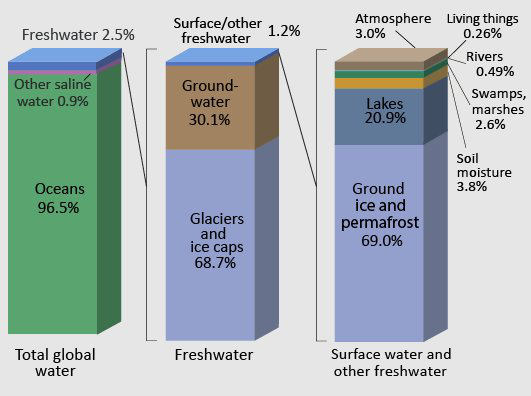
| Type | Percentage |
|---|---|
| Oceans | 96.5 |
| Other saline water | 0.9 |
| Freshwater | 2.5 |
| Type | Percentage |
|---|---|
| Glaciers and ice caps | 68.7 |
| Groundwater | 30.1 |
| Surface/other freshwater | 1.2 |
| Type | Percentage |
|---|---|
| Ground ice and permafrost | 69 |
| Lakes | 20.9 |
| Soil moisture | 3.8 |
| Atmosphere | 3 |
| Swamps, marshes | 2.6 |
| Rivers | 0.49 |
| Living things | 0.26 |
Systems Thinking and the Hydrologic Cycle
Systems Thinking and the Hydrologic Cycle
Throughout this course, we will be dealing with complex systems and “Systems Thinking”. What is Systems Thinking, you may ask? According to Peter Senge, author of The Fifth Discipline Fieldbook, “Systems thinking is a way of thinking about, and a language for describing and understanding, the forces and interrelationships that shape the behavior of systems”. Some systems are very complex, but all systems can be simplified to help understand the relationships between systems components. Systems can be "modeled" to help investigate their dynamics. We do not expect you to become system modelers, per se, but simple models can begin to help you understand how changes in one parameter might influence changes in another. Let's consider a simple system in which we have a bathtub, fed by a faucet, and drained at its lower level. We could diagram this simple system as follows…

In this system there is a reservoir (the bathtub), an input (the faucet), and an output (the drain). The relationships in this system are simple and, hopefully, intuitive. If you want to run water into the tub for a long time to keep it quite warm, but not have it run over, what are your choices? You could keep the drain closed and run a very slow trickle of warm water into the tub from the faucet, letting it fill gradually, or, you could fill the tub quickly to some level, then open the drain to allow water to leave the tub at the same rate as it is being added to prevent further rise in the water level. Cold water is more dense than warm, so perhaps cooler water would drain preferentially and this would keep the tub water warmer overall. You could also evaluate the time it would take to fill the tub, or drain it, knowing the tub volume (gallons), the maximum input rate through the faucet (gallons/minute), and the maximum drain rate (gallons/minute).
Learning Checkpoint
Let's try a couple of simple model calculations to get you thinking about systems dynamics. First, we should establish some volumes and rates for this simple system. The tub (reservoir) will hold 30 gallons of water. The input and output values are outlined below:
1) If the faucet (input) will supply 3 gallons of water per minute, and the drain is closed (no output), how long will it take to fill the tub to the brim with water if the tub is empty to begin with?
ANSWER: The tub will fill in 10 minutes (30 gallon capacity divided by 3 gallons per minute input).
2) If the faucet supplies 3 gallons per minute, the tub is empty to begin with, but the drain allows 3 gallons per minute to leave the tub, how long will it take the tub to fill?
ANSWER: The tub will never fill because it starts empty and input = output!
3) If the faucet supplies 3 gallons per minute, the tub is empty to begin with, and the drain allows 1 gallon per minute to escape, how long will it take to fill the tub?
ANSWER: The tub will fill in 15 minutes (30 gallons capacity divided by (3 gallon/minute input minus 1 gallon per minute output).
Hydrologic Cycle
Hydrologic Cycle
The movement of water between these reservoirs, primarily driven by solar energy influx at the Earth’s surface, is known as the hydrologic cycle.

| Component | Fluxes in 103 km3/ year |
|---|---|
| Evaporation | 436.5 |
| Precipitation | 391 |
| Groundwater Runout | 45.5 |
| Evapo-transpiration | 65.5 |
The hydrologic cycle is a conceptual model that describes the fluxes of water between the oceans, surface water bodies (lakes, rivers, and streams), groundwater in subsurface aquifers, the atmosphere, and the biosphere. One important aspect of the cycle is that no water is gained or lost: water moves between reservoirs but the total mass remains the same. Another way to say this is that the water that currently exists on Earth is the same water that has been here since the time the Earth formed. (Technically, there are small fluxes of water from the Earth’s interior to the surface and atmosphere through volcanism and venting, and small influxes of water from comets and debris, but these are negligible in comparison to the mass of water in the primary reservoirs shown above.)
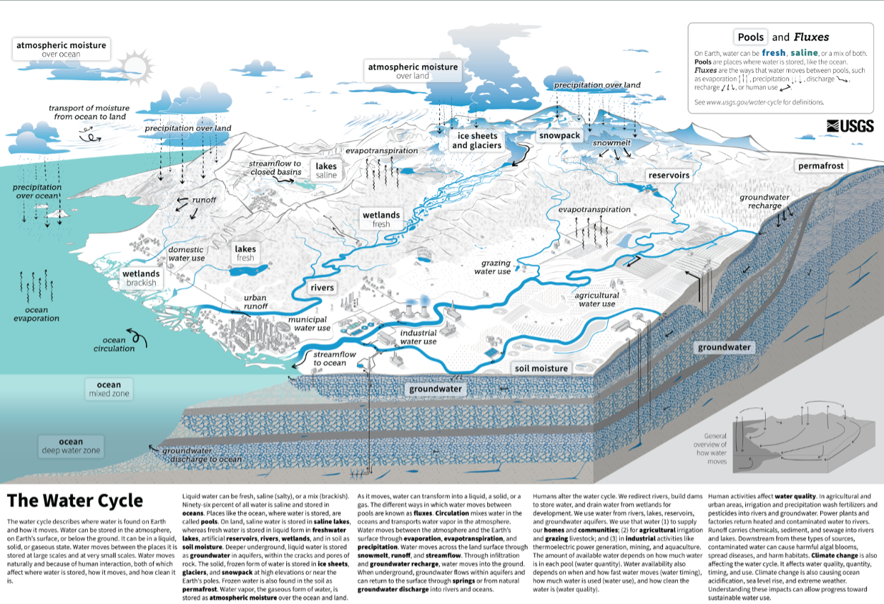
Activate Your Learning
1. There are five processes that control the movement of water between reservoirs in the hydrologic cycle. Looking at Figure 6 above, what do you think they are? Name as many as you can.
ANSWER: The processes include evapo-transpiration, precipitation, runoff, infiltration, and groundwater outflow. Read on for further description.
The movement of water between reservoirs, or the “limbs” of the hydrologic cycle includes five primary processes:
- Evapo-transpiration: the movement of water from oceans or land to the atmosphere, through the combined processes of evaporation and transpiration. Evaporation and transpiration both involve a change in state, from liquid to vapor, which requires an input of energy. Evaporation is simply the change from liquid to vapor as a result of molecular motion, and is affected by temperature and ambient humidity. Transpiration is the movement of water to the atmosphere by plant respiration. In most terrestrial basins, transpiration is the dominant process by which water moves from the Earth’s surface to the atmosphere, whereas over lakes and the oceans, evaporation dominates.
- Precipitation: the movement of water from the atmosphere to the land surface or oceans, in the form of rain, snow, sleet, ice pellets, etc... Precipitation involves a change in state from vapor to liquid, known as condensation. This change in state releases heat energy. After precipitation falls on the land surface, it may flow into surface water bodies (lakes or streams), or percolate through soils and rock into the groundwater system.
- Runoff: the movement of water from the land surface to the oceans in streams or rivers.
- Infiltration: the percolation of water from the land surface or from surface water bodies through soils and into the subsurface. Water that infiltrates becomes part of the groundwater system, and is also known as groundwater recharge.
- Groundwater outflow, also known as subsea outflow: the seepage of water from the groundwater system directly into the oceans. The flux of groundwater outflow is the least constrained component of the hydrologic cycle, and is often estimated by balancing the other fluxes in the cycle.
Because the changes in state that accompany evaporation and precipitation also take in and release energy, the movement of water through the hydrologic cycle is paralleled by redistribution of heat and energy.
Uneven Distribution
Uneven Distribution
Why is water distributed unevenly across the Earth’s surface?
As you probably know, things are far more interesting than a hypothetical case of evenly distributed precipitation! Both precipitation and evaporation vary widely over the Earth’s surface. This unequal distribution of water on the planet drives a diversity in climate and ecosystems (or biomes); water availability for human life, industry, and agriculture; and is fundamentally and intimately tied to the history of politics, economics, food production, population dynamics, and conflict – both in the U.S. and globally.
The abundance of water in some areas and scarcity in others follows systematic and predictable patterns. As part of this module, we’ll explore the physical processes that shape the overall distribution of precipitation - and thus water resources.


Learning Checkpoint
Note: The questions below are not graded. They may show up as summative evaluation questions on mid-term or final exams.
1) Look at Figure 7 above. What is the annual mean precipitation in Southern Nevada?
- 32 in/yr
- greater than 80 in/yr
- 0 in/yr
- 4-8 in/yr
ANSWER: d. 4-8 in/yr
2) Look at Figure 7 above. What is the annual mean precipitation in Coastal Washington State?
- a. 32 in/yr
- greater than 80 in/yr
- 0 in/yr
- 4-8 in/yr
ANSWER: b. greater than 80 in/yr
3) Why do you think Nevada and Eastern Oregon are deserts?
- a. They are far North of the equator.
- They are far from the ocean.
- They are in the rain shadow of mountains.
- They are subject to large annual temperature fluctuations.
- They are at high elevation.
ANSWER: c. They are in the rain shadow of mountains.
4) Look at Figure 8. What do you think is the global pattern of precipitation?
- a. It rains most South of the equator.
- There is East-West "banding" of climate/precipitation.
- There is North-South "banding" of climate/precipitation.
- There is snow in the Southern Hemisphere year-round.
ANSWER: b. There is East-West "banding" of climate/precipitation.
Note the contrasting patterns in the two images in Figure 8 above, based on global satellite coverage. Vegetation in the southern hemisphere, which has relatively more ocean area (and less land area) than the northern hemisphere, changes little seasonally, whereas vegetation distribution in the northern hemisphere undergoes large changes. Why is that? There are probably two impacts on vegetation distribution—precipitation and temperature. Examine the figure below that illustrates the available moisture seasonally (summer vs. winter) and compare to the distribution of vegetation for the same seasons. Think about the role of temperature, precipitation, and soil moisture (water availability to plants), as well as the availability of sunlight for photosynthesis. Yes, there is a more complex relationship between plant growth and other factors, but the hydrologic cycle plays a major role.


Relative Humidity
Relative Humidity
The explanation for spatial variations in precipitation centers on the concept of relative humidity. The relative humidity is the water vapor pressure (numerator) divided by the equilibrium vapor pressure (denomator) times 100%. The equilibrium vapor pressure occurs when there is an equal (thus the word equilibrium) flow of water molecules arriving and leaving the condensed phase (the liquid or ice). Thus there is no net condensation or evaporation (Alistair Fraser, PSU).
Now, if the water vapor pressure is greater than the equilibrium value (numerator is greater), there is a net condensation (and a cloud could form, say). And that is not because the air cannot hold the water, but merely because there is a greater flow into the condensed phase than out of it.
Relative humidity describes the amount of water vapor actually in the air (numerator), relative to the maximum amount of water the air can possibly hold for a given temperature (denominator). It is expressed as a percentage:
If the relative humidity (RH) is 100%, this means that condensation would occur. On a typical hot muggy summer day, RH might be around 60-80%. In a desert, RH is commonly around 15-25%.

One important consequence is that when air masses change in temperature, the relative humidity can change, even if the actual amount of water vapor in the air does not (the numerator in our equation, which is defined by the saturation curve, stays the same, but the denominator changes with temperature). Figures 11-13 below show an example of this process. As the air cools, the relative humidity increases. If the air mass were cooled enough to become saturated (hit the solid black curved line), condensation would occur. This temperature is called the dew point.
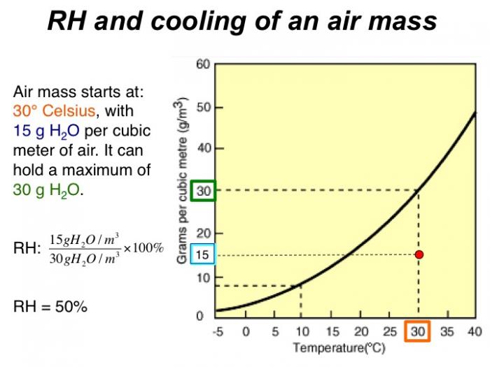
Air mass starts at 30 degrees Celsius, with 15 g H2O per cubic meter of air. It can hold a maximum of 30 g H2O. RH = 50%

With cooling, air still contains 15 grams H2O per cubic meter of air. But it can now only hold a maximum of 22 grams H2O. RH = 68%

With cooling, air still contains 15 grams H2O per cubic meter of air, equal to the maximum it can hold. This temp. is called the dewpoint. RH = 100%!
In the same way, changes in relative humidity occur when warm moist air is forced to rise or, conversely, when cool dry air descends. For example, when an air mass moves over mountains, it cools as it rises, and when it reaches the dewpoint, water will condense. This forms clouds, and if the air mass cools enough, the condensation becomes rapid enough to form precipitation.
The Orographic Effect
The Orographic Effect
To take the concept of relative humidity outdoors, let's consider why it rains in some areas and we have deserts in others. There are two primary reasons for this. Both are related to the transport, rise, and fall of air masses that lead to temperature changes, and ultimately in the amount of water vapor that the air can hold. These are the orographic effect, and atmospheric convection.
In both cases, cooling and warming of air masses occurs because they are forced upward or downward in the atmosphere. The decrease in air temperature with elevation is known as the atmospheric (or adiabatic) lapse rate, as shown below, and is related to decreasing air density and pressure with increasing altitude (as air rises, it expands due to decreased pressure, leading to lower temperature). A typical average lapse rate is around 7° C per km of altitude change. If an air mass begins rising and has not reached the dewpoint temperature, it follows a dry adiabatic lapse rate, with the rate of cooling due nearly entirely to decreasing pressure, as shown in Figure 14. Once the airmass temperature reaches the dewpoint during continued rise, water droplets begin to condense (forming clouds) and the airmass follows a moist adiabatic lapse rate (Figure 14), for which the rate of cooling with elevation decreases because of the addition of some offsetting heat to the airmass from the process of condensation (termed latent heat).

The orographic effect occurs when air masses are forced to flow over high topography. As air rises over mountains, it cools and water vapor condenses. As a result, it is common for rain to be concentrated on the windward side of mountains, and for rainfall to increase with elevation in the direction of storm tracks. With continued cooling past the dewpoint, the amount of water vapor in the air cannot exceed saturation, so water is lost from the air via condensation and precipitation.
On the leeward side of mountain ranges, the opposite occurs: the air descends and warms. As it does so, it is capable of holding more water vapor (recall the saturation line in the relative humidity plot above). However, there is no source of additional water, so the descending air mass increases in temperature but the amount of water vapor remains constant. Because the air has lost much of its original water content, as it descends and warms its relative humidity decreases. These areas are called rain shadows and are commonly deserts. You’ve probably noticed this same process in action when you heat your house or apartment in the winter – warming the cold air leads to dry conditions – one of the reasons people often put water pots or kettles on their wood stoves.
Orographic Effect In Action
The animation below shows an airmass trajectory superimposed on a Google Earth image of western North America. The point of this animation is to provide an explanation of the orographic effect and the changes in temperature and water content of an airmass passing over several mountain ranges. The animation shows the "rain shadow" effect that results in desert regions behind large mountain ranges. An inset graph at bottom right illustrates combinations of temperature (x-axis) and moisture content (y-axis) in grams per cubic meter of the air mass as it passes over various topographic features on the land surface.

Atmospheric Convection: Hadley Cells
Atmospheric Convection: Hadley Cells
There is a second, larger-scale effect that also plays a key role in the global distribution of precipitation and evaporation. Fundamentally, these patterns are also explained by the rise and fall, and cooling and warming of air masses – as is the case with the orographic effect – but in this case, their movement is a result of atmospheric convection rather than transport over topographic features.
As you have seen, there are regular climate and precipitation bands on the Earth – latitudes where most of the Earth’s tropical and temperature rainforests, deserts, polar deserts (also known as tundra) tend to occur. This global pattern – along with prevailing global wind patterns and storm tracks, are driven by atmospheric convection.
It all starts with solar radiation. Because of the Earth’s curvature, the tropics (between 23.5° N and S latitude) receive a larger flux of solar radiation per unit area on average than higher latitudes. Because the Earth’s axis is tilted, during Northern hemisphere summer, the peak influx of solar radiation occurs at 23.5° N latitude. During the Southern hemisphere summer, the maximum occurs at 23.5° S. (Incidentally, these latitudes define the tropics of Cancer and Capricorn.) Annually, the highest flux of solar energy per unit area occurs at the equator, as shown below.
As a result, the air around the equator becomes warmest. It holds quite a bit of water, too – based on the fact that, as you’ve seen above, warm air has a higher capacity to carry moisture.
Video Review: Global Atmospheric Circulation (2:24)
Take a few minutes to review the video below to help you understand Global Circulation a little better.
In this animation, we're going to look at global wind patterns and talk about the reasons why the air circulates the way it does and also patterns of rising and sinking air and how that relates to precipitation. The engine that drives it all, I guess you could say, is the intense heating by the Sun that occurs only in the equator areas where the sun is shining is at a very high angle of incidence and this hot air near the equator being less dense Rises upward. It rises up, going to move toward the poles and then it gradually sinks at about 30 degrees north and south latitude. So we create these big spinning circles of air that we call the Hadley cells near the equator where the air is rising it loses its ability to hold moisture and you get a band of high rainfall and low pressure because there's air leaving the equator where the air sinks. In these, it belts at around 30 degrees north and south you get high pressure sinking air which creates areas of clear skies and desert climates now as this air circulates and tries to flow back toward the equator along the surface of the earth or as some of it heads toward the North Pole or toward the South Pole. The Coriolis effect, the spin of the earth, causes it to bend and turn and it's going to create the too big wind belts that prevail on our earth two out of three the trade winds north-northeast trade winds and southeast trade winds and then the prevailing westerlies. Now these winds curve the way they do because of the Coriolis effect the winds curve to the right of their path north of the equator, they curve to the left of their past south of the equator, and they end up flowing to the from east to west or from west to east. Now the other big factor is what's happening at the poles. At the poles the air is cold and the cold air wants to sink and as that cold polar air sinks it heads toward the equator and it bumps into this air heading toward the pole here and toward the South Pole here and it creates an area of rising air and again rising air produces high precipitation belts at about 60 degrees north and about 60 degrees south latitude. At the polls themselves, the precipitation is quite modest because the air is sinking and that creates low precipitation.
Energy Balance
Energy Balance

On average regions near the equator receive light at 90°. high latitudes receive light at low angles. Light energy is more concentrate near the equator. In other words, there is a greater flux per unit area (W/m2)


The differential heat input from solar radiation input and loss by infrared radiation is a critical part of maintaining equability (relatively low gradients in temperature from low to high latitudes) on the Earth. The energy balance figures indicate that above about 40 degrees North and South (e.g., the latitude of New York City) of the equator the loss of heat by radiation (infrared), on average, exceeds the input of heat from the sun (visible). What does that imply for our climate? One might think that this should result in permanent snow or ice above this latitude. Right? Indeed, during the last glacial epoch, about 21 thousand years ago, thick continental ice sheets extended to nearly 40 degrees North in North America (just north of I-80). But normally, because of the heat gradient created by the imbalance between solar input and infrared radiation, the atmosphere (and ocean) is set in motion to redistribute heat from low to high latitudes. Otherwise, the tropics would be excessively hot and the high latitudes excessively cold—at all times. Next, we will see how this circulation works.
Global Wind
Global Wind
As this warm air rises due to its lower density, it cools. Once it cools past the dewpoint, condensation occurs and clouds form. With continued rise and cooling, the air cannot hold the moisture and precipitation falls.
In response to that rising air, surface air must flow in to fill the vacated space. The rising air results in a low-pressure center. This is why when you hear about low pressure in the forecast, is typically associated with rising air masses and therefore with crummy weather. The air rushing in toward the equator defines the trade winds. These winds converge on the equator but blow to the West because of Earth’s rotation. This rotational effect is known as the Coriolis effect. We won’t get into that in detail here, but if you are interested, check out the video below.
Video: The Coriolis Effect (02:43)
[thundering]
NARRATOR: Picture a circle. Here's its center, here's point A, and here's point B. Point A is twice the distance from the center of the circle than point B. Oh, yeah, and it spins from its center. In two seconds, both points do one full revolution. But to go all the way around, point A has to go this far, while point B only has to go this far. And we all know if something travels a greater distance in a shorter amount of time, it must be going faster. So, point A must be moving faster than point B.
Okay, now swap out this flat circle for the Earth, and the same thing is true. All points closer to the center, say like someone in Greenland, will be spinning slower when compared to points spinning further away from it, say like people in Brazil, closer to the equator. So, if we look at it all flattened out, we can picture something like this. Arrows at the equator travel faster than arrows at the 45 degree line, like we just observed. Now, imagine you're a cloud that formed here on the equator. You'll have the same velocity as the Earth. But then a gust of wind sweeps you to the north, where the Earth isn't spinning as fast.
Due to inertia, your speed remains the same. You don't get any faster, but everything around you is literally traveling slower, so you, relative to the ground, move ahead of everything else. If you're a cloud that forms at the 45 degree line, you'll also have the same speed as everything around you. But if you drift down to the equator, you'll be moving slower than the ground underneath you, so you'll fall behind. And the same thing for the Southern hemisphere. Moving towards the equator always results in falling behind, while moving away results in pushing ahead.
Okay, now imagine a low-pressure cell. That means all the air around it will get sucked into the center. But the air coming from the equator will be traveling faster, so it will deflect to the right, while the air coming from the poles will be moving slower, so they'll fall behind and deflect to the left. What this results in is a circular air current spinning counterclockwise. And that's exactly what hurricanes are, low pressure cells spinning because of the Coriolis effect. Moving this example down to the Southern hemisphere, things are reversed. A low pressure cell will still suck in the surrounding air, but now the air coming from above will be moving faster, again deflecting to the right, while the air coming from below is moving slower, again falling behind by moving to the left.
This results in a clockwise spin, which is why storms spin, which is why storms in the Southern hemisphere spin this way. And that's about it. It's a short video, and that's the point. I hope you got what you came for. And the Coriolis effect doesn't really influence toilets. They're just really too small. And the direction of the spin more depends on the placement of jets inside the toilet. But that's it. That's the Coriolis effect. If you like this short and to-the-point video, give this video a like. And if you want to see more videos like it, why not subscribe? I'll be back next week with another video. So until then, thanks for watching.
These flows drive convection cells, with dimensions that are controlled by the viscosity and density of air, and by the thickness of the atmosphere. The air that rose from the equator flows North and South at the top of the cell and eventually descends at around 30° N or S latitude. As the cool, now dry air descends, it warms. Sound familiar?
Just as occurs when air descends on the leeward side of mountain ranges and causes rain shadows, the amount of water that the descending and warming air could hold increases. But there is no additional moisture to be found, so the actual amount of water vapor in the air mass remains more-or-less fixed. These descending limbs of the Hadley cells form high-pressure centers and would be regions where persistent dry conditions should prevail – leading to the Earth’s desert belts that include the Gobi, Sahara, Arabian, and the Australian Outback (not just a steakhouse!).
The equatorial convection cells are known as Hadley Cells. There are two more in each hemisphere, also driven by the uneven distribution of incoming solar radiation density; these are Farrell and Polar cells. Check out the diagram of this process below.

Global Wind Explained
Global Wind Explained
The illustration below portrays the global wind belts, three in each hemisphere. Note that the U.S. lies primarily in the Westerly Wind Belt with prevailing winds from the west. Each of these wind belts represents a "cell" that circulates air through the atmosphere from the surface to high altitudes and back again. The cells on either side of the Equator are called Hadley cells and give rise to the Trade Winds at Earth's surface. How do we explain this pattern of global winds and how does it influence precipitation?
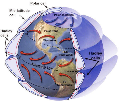
We'll start at Earth's equator, where solar radiation is the highest year around. Air near the equator is warmed and rises because it is less dense (mass/unit volume) than the air around it as shown in Figure 21 below.
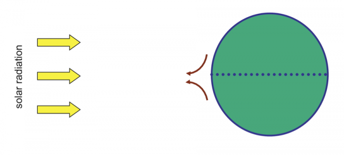
The rising air creates a circulation cell, called a Hadley Cell, in which the air rises and cools at high altitudes moves outward (towards the poles) and, eventually, descends back to the surface. The continual heating and rise of air at the equator create low pressure there, which causes air to move (wind) towards the equator to take the place of the air that rises. On the other hand, sinking air creates high pressure at the surface where it descends. A gradient of pressure (high to low) is formed that causes air to flow away from the high and towards the low pressure at the surface.


The Earth would have two large Hadley cells if it did not rotate. But, because it does rotate, the rotation of the Earth leads to the Coriolis effect. You should view the short video on this so-called "effect" or "force." (The Coriolis Effect [30]). Without going into detail as to why rotation creates this apparent force, the Coriolis effect causes winds (and all moving objects) to be deflected:
- to the right in the Northern Hemisphere
- to the left in the Southern Hemisphere
The Coriolis effect causes winds to deflect as they travel within circulation cells and results in the two large hypothetical Hadley cells breaking into six smaller cells, which looks something like the diagram below (and the first figure in this series).

Ok, so, we now have some idea about the origin of global wind systems that result from pressure gradients at Earth's surface. How does this produce precipitation, and where? Precipitation occurs where moisture-laden air rises, either by heating at the equator or by running up and over a more dense air mass. As the rising air cools its capacity to hold water decreases (relative humidity increases) and, at some point, saturation with respect to water vapor is reached. Then, condensation--clouds and rain!

The diagrams above and below portray just the Hadley cell circulation, that is driven by heating in the equatorial region. On the surface, wind moves away from high pressure (High) and toward low pressure (Low). Convergence occurs near the equator (winds blow in towards one another) and Divergence occurs under the descending air that forms high-pressure belts. The final figure (Figure 26) shows all six cells diagrammatically, along with the pressure variations at the surface of the Earth and zones of typical wet and dry belts. Note particularly the dry belts near 30 degrees North and South.


| Latitude | Barometric Pressure | Precipitation | Surface winds |
|---|---|---|---|
| 90° | High | Dry | Divergent |
| 60° | Low | Wet | Convergent |
| 30° | High | Dry | Divergent |
| 0° | Low | Wet | Convergent |
Unit 2: Physical Hydrology
Unit 2: Physical Hydrology
Overview
This section of the course outlines the distribution of water on land and its organization into watersheds and major river systems. Rivers are one of the major concentrated sources of fresh water that can be extracted for human use for agriculture, industry, and drinking water, prior to flowing into the oceans. Another potential source of fresh water is so-called "groundwater," which consists of water held in subsurface rock units with varying potential for storage and yield. This helps us explain the distribution and dynamics of water at the surface and in the subsurface of the Earth. At times the water distribution through river systems is either subject to a deficit of water (drought) or surfeit (flood), subject to variations in climate or to unusual meteorological events. Humans attempt to control these variations by constructing dams to regulate river flow and store water for use, particularly in dry regions. However, dams, although providing water and power, have consequences for the environment.
This section provides a more detailed overview of water transport and availability and highlights issues with water storage in reservoirs and in the subsurface. In subsequent modules, we learn how water availability influences civilizations, both past and present.
Modules
- Module 3: Rivers and Watersheds [31]
- Module 4: Flood and Drought [32]
- Module 5: Dam It All! [33]
- Module 6: Groundwater Hydrology [34]
Unit Goals
Upon completion of Unit 2 students will be able to:
- Describe the two-way relationship between water resources and human society.
- Explain the distribution and dynamics of water at the surface and in the subsurface of the Earth.
- Synthesize data and information from multiple reliable sources.
- Interpret graphical representations of scientific data.
- Identify strategies and best practices to decrease water stress and increase water quality
- Thoughtfully evaluate information and policy statements regarding water resources
- Communicate scientific information in terms that can be understood by the general public
Unit Objectives
In order to reach these goals, the instructors have established the following learning objectives for student learning. In working through the modules within unit 1 students will be able to:
- Explain the processes by which precipitation accumulates, moves through, and is transported out of a watershed.
- Describe the physical components of a river channel and floodplain.
- Define the different types of sediment transported in rivers and explain to a first-order the physical processes governing sediment transport.
- Explain the various techniques by which humans attempt to restore hydrologic, geomorphic and ecological functions of rivers and watersheds.
- Explain the role of ‘extreme events’ in the water cycle and distribution of water on Earth’s surface.
- Explain a few basic techniques for organizing and analyzing hydrologic data, including time series plots and histograms.
- Articulate the difference between a forecast and a prediction and provide examples of each.
- Define the term flood, describe the factors that influence the magnitude of a flood, and explain the implications of floods for society and ecosystems.
- Compute the probability that a flood or drought of a given Recurrence Interval might occur (e.g., the 100 year flood).
- List the different types of droughts and be able to explain the basic implications of each for society and ecosystems.
- Define the terms stationarity and non-stationarity and explain the implications for flood predictions.
- Explain the reasons why dams are built, and how these differ in different locations
- Weigh the advantages and drawbacks of large dams
- Consider the causes of conflict and controversy across national borders associated with large dam projects
- Explain the issues caused by sediment trapping behind dams
- Debate the justification for building and rationale for removing dams
- Identify an artesian well and predict where artesian wells will be found
- Distinguish between porosity and permeability
- Associate hydraulic properties with given rock types
- Interpret relative permeability from a well productivity diagram
Module 3: Rivers and Watersheds
Module 3: Rivers and Watersheds
Overview
In this module, we will investigate the processes by which precipitation accumulates in, moves through, and is transported out of a landscape. We will especially focus on flow of water in streams and rivers, including how these important features form and change over time. The goals of the module are to develop an understanding of the water cycle at the watershed scale, as well as to explore the variety of rivers that exist on Earth’s surface, develop an understanding of how those rivers change over time and learn how to measure the amount of water transported by a stream or river. As part of this, you’ll come to understand how water is conveyed to a river, and become familiar with terms such as flow duration, sediment transport, channel and floodplain morphology, and stream and watershed restoration.
Goals and Objectives
Goals and Objectives
Goals
- Explain the distribution and dynamics of water at the surface and in the subsurface of the Earth
- Synthesize data and information from multiple reliable sources
- Interpret graphical representations of scientific data
Learning Objectives
In completing this module, you will:
- Identify and describe the processes by which precipitation accumulates, moves through, and is transported out of a watershed
- Describe the physical differences between terrestrial and stream systems
- Qualitatively evaluate stream gage data
- Visually identify various common channel morphologies in Google Earth
- Describe physical characteristics of a river channel, including stream order, number of channels, and sinuosity
- Analyze how topography influences water movement over land
Water Moves Through the Landscape
Water Moves Through the Landscape
The most obvious way water moves through a landscape is via stream and river channels. There is no formal definition to distinguish between brooks, creeks, streams, and rivers, but generally speaking, the former terms refer to smaller waterways and the latter refer to larger waterways. The terms stream and river are often used interchangeably. There are over 3.5 million miles (5.6 million kilometers) of streams and rivers in the US. If all the streams and rivers throughout the US were lined up one after the next, they would extend the distance from Earth to the moon and back...seven times! That is an incredible length of streams to be monitored, protected, regulated, and (occasionally) repaired by federal, state and local agencies, as well as industry and non-profit organizations and individuals. In addition, streams sculpt much of the surface of the Earth, forming a multitude of beautiful patterns and awe-inspiring features, as shown in Figure 1.

Channel Networks and Watersheds
Channel Networks and Watersheds
Streams naturally assemble themselves into surprisingly well-organized (quasi-fractal) networks. Figure 2 shows a typical channel network where many small streams converge to make progressively larger streams. The smallest streams in the network, which have no other streams flowing into them, are referred to as first order streams. When two first order streams meet, a second order stream is formed. When two second order streams meet, they form a third order stream, and so on. According to this conventional stream ordering system, first developed by Horton (1945) and refined by Strahler (1957), when a smaller order stream (e.g., first order) meets a larger order stream (e.g., second order), the resulting stream retains the order of the larger stream (in this case, second order).
Each stream has a watershed, also known as a ‘river basin’ or ‘catchment’ because it is the land that ‘catches’ precipitation and funnels it towards the stream. The watersheds of two first order streams are outlined with grey dashed lines in Figure 2. The watershed of a second order stream is outlined in black dashed lines and encompasses the two first order watersheds. The solid black outline in Figure 2 shows the watershed boundary for the fourth order watershed, which encompasses all other watersheds nested within it. The right side of Figure 2 shows the Mississippi River watershed highlighted in green, with the Missouri River watershed nested within it, highlighted in orange. By the time the Mississippi River reaches New Orleans, it is a tenth order stream (though only a few of its largest tributaries are shown in Figure 2), and drains more than one-third of the contiguous US.
The concept of connectivity between rivers and their watersheds will come up again towards the end of this module in the context of restoration. If a particular stretch of stream is impaired for one function or another (e.g., fish habitat has been degraded), in some cases it makes sense to ‘fix’ that specific stretch of river, while in other cases the impairment is simply a symptom of problems higher up in the watershed, so the ‘fix’ may need to be applied at that location in the watershed before human intervention or natural processes can begin to repair the impaired stream. Such is the way that watersheds and streams are connected.

Watersheds are Complex Systems
Watersheds are Complex Systems
When you look around, you see that the world is full of systems…assemblages or combinations of things that form a functional unit. Some systems are human-made, others are made by nature. Some systems are simple, meaning the way they work is straightforward and the outputs from the system are easily predictable. Other systems are complex, meaning they often have many parts that interact, often in non-linear ways, making the outputs from those systems more difficult to predict.
For example, a coffee maker is a pretty simple system. You put in 8 cups of water and two cups of coffee grounds and (assuming you put them in the right places), you turn the machine on and get ~8 cups of coffee. If you change the amounts of either of the inputs, it is pretty easy to predict the impacts on the coffee you brew.
Watersheds are not such a simple system. They are incredibly complex. One example can be seen in how the relationship between rainfall and runoff changes throughout the year. In a simple system, you would expect a constant relationship between incoming rainfall and outgoing flow. For example, a 1-inch rain event should translate to a stormflow hydrograph that might last 2 days and peak at 1000 cfs. But this isn’t what we see. Figure 3 shows streamflow (blue line, values on the left axis) and precipitation (orange bars, values on the right axis) from March through September 2008 for the Maple River near Rapidan, Minnesota. Precipitation is relatively evenly distributed throughout the year. As you can see, in April and May, rainfall events that are 0.5 to 1 inch result in relatively high flows (1000 to 1500 cfs). However, in July, August, and September, similar rainfall events hardly elicit any flow response whatsoever! Why do we see such non-linear behavior?

Activate Your Learning
The Maple River example above is a relatively extreme example of changes in rainfall-runoff relationships because soils are relatively wet (and therefore can’t absorb much of the incoming rainfall) in the spring and there is very little vegetation to intercept or evapotranspire water (the watershed is covered in row crops that don’t grow much before mid-June). In contrast, the row crops are in full effect by mid-summer and early fall and therefore they dry out the soil, intercept some incoming rainfall and evapotranspire most of the rest of the incoming rainfall…so it never gets to the channel! But similar phenomena can be seen in other watersheds. Find precipitation and streamflow data for a watershed of interest to you (from the USGS website, NRCS SNOTEL website, or NWS website). Plot them as shown in Figure 3. How well does flow correlate with precipitation? Are there seasonal differences? Differences from year to year?
ANSWER - NEED ANSWER OR TALKING POINTS.
Watersheds comprise many interacting parts. Figure 4 (top panel) is one way to represent various ‘parts’ that might be considered to comprise the watershed. While this is clearly a very simple view of this complex system, it is useful to take a “crude look at the whole”, a term coined by Nobel Prize-winning Physicist Murray Gell-Mann, as a starting point. When one component of the system is systematically changed, it may have direct as well as indirect impacts that propagate through the system. For example, changes in precipitation, snowmelt regime, or water storage may change streamflow. This altered streamflow has direct effects on river channel morphology, sediment transport, riparian vegetation, water quality, nutrient processing, and biodiversity, as indicated by the yellow arrows in the middle panel of Figure 4. But there are other interactions within the system, feedbacks that are indicated by purple arrows in the bottom panel of Figure 4. So to predict impacts of the changes in flow on aquatic biodiversity you would have to take into account not only the direct effects (yellow arrow between flow and aquatic biodiversity, but also the indirect effects associated with changes in channel morphology. This concept is also relevant in the context of watershed ‘restoration’. If a particular stretch of stream is impaired for one function or another (e.g., fish habitat has been degraded), in some cases it makes sense to ‘fix’ that specific stretch of river, while in other cases the impairment is simply a symptom of problems higher up in the watershed, so the ‘fix’ may need to be applied at that distant location in the watershed before human intervention or natural processes can begin to repair the impaired stretch of stream.
These notions of complex feedbacks and cascading effects greatly complicate the process of predicting what impacts human activities or natural disturbances within a watershed might have downstream. We’ll come back to this theme of system dynamics and complexity throughout the course.


Streams
Streams
Streams are the most obvious way that water is moved through a watershed because we see them all over. But there are many other means by which water moves, as discussed in module 2. Figure 5 illustrates the various stocks (places were water is stored, even if only temporarily) and fluxes (mechanisms by which water moves) of water that may exist within any given watershed. For example, one raindrop might fall onto vegetation (called interception) and subsequently be evaporated back up into the atmosphere. Another raindrop might fall onto the soil surface and then runoff the surface into the stream channel or it might infiltrate down into the soil. Once in the soil, the water might further percolate down into the groundwater, where the soil or rock is saturated with water. Alternatively, once in the soil, the water might travel downhill within the soil and runoff into the stream or it might be taken up by vegetation and transpired back into the atmosphere. Estimating and predicting which, and to what extent, water travels through these pathways is an active field of hydrologic research and is also vitally important for environmental management and policymaking, as certain pathways may be more or less prone to filtering or polluting water along its journey to the place where you might want to use it for drinking, irrigating, fishing, swimming or the myriad other purposes for which we need water.

River Flow Changes Over Time
River Flow Changes Over Time
The amount of water moving down a river at a given time and place is referred to as its discharge, or flow, and is measured as a volume of water per unit time, typically cubic feet per second or cubic meters per second. The discharge at any given point in a river can be calculated as the product of the width (in ft or m) times the average depth (in ft or m) times average velocity (in ft/s or m/s).
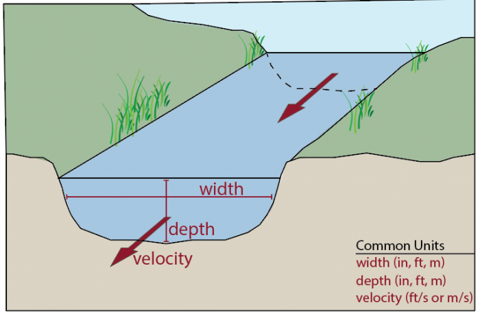
The vast majority of rivers are known to exhibit considerable variability in flow over time because inputs from the watershed, in the form of rain events, snowmelt, groundwater seepage, etc., vary over time. Some rivers respond quickly to rainfall runoff or snowmelt, while others respond more slowly depending on the size of the watershed, steepness of the hillslopes, the ability of the soils to (at least temporarily) absorb and retain water, and the amount of storage in lakes and wetlands.
Video: How to Measure a River (8:35)
Good morning. I'm Barry, I'm Ben. We're the Geography Men.
Ben: Now today I'm going to be showing you how to measure the discharge of a river. Now for this what you're going to need is a tape measure, a meter stick, a flowmeter, a couple of stakes to help you out, and a recording sheet to record your data.
So the first thing you're going to want to measure is the width of the river. Now as I said before, for this you're going to need a tape measure, preferably let's say a 30-meter tape measure. Now from the left-hand bank, you want to have your 0-end of your tape measure. The easiest way to do this is to tie it to something or to use a stake in the ground. Now here I'm going to tie it to this root just to help me out. Now you want to stretch the tape measure across the river, making sure that it is tight across the surface of the water. You do not want to allow it to go slack, otherwise, that tape is going to get carried off by the river and you are going to get a false measurement of the width of your river.
Now that you have your tape set across your river, you want to record where the river begins, where the water meets the bank. Record on the other edge, on the other bank, where the water meets the bank, and then work out that distance from one bank to the other.
With this river here, our left-hand bank starts at 1 meter 60 and our right-hand bank ends at 5 meter 60, giving us a width of our river of 4 meters. Now the next thing we need to do with that width is we need to divide it by 11, in order to work out the intervals at which we need to work out the depths of our river. The reason we divide it by 11 is because we're going to take a measurement at each of the banks. This will give us 10 intervals across our river to take our depth.
Now for our depth, we're going to want to use a meter stick. Now with the meter stick, there's some very simple things that you need to remember. Number one, make sure the zero end of the stick is at the bottom of the river. You don't want to have it upside down and be getting readings of 80 or 90 centimeters. You want to turn the meter stick parallel to the flow of the water, so as that meter stick does not block that flow of the water giving you two false values on either side. Starting at the bank, place that meter stick into the water until it reaches the bed of the river. Now you want to take a reading and you want to convert that reading straight into meters, as you want the same units for each of your measurements. So here we have 25 centimeters, so we have naught .25 meters. Find your next interval on the tape and do exactly the same again. We have naught .21. Naught .24. And you would then follow that across the river until you reach the right-hand bank.
Now the final measurement you want to take at your site, to work out the discharge of the river, is a flow reading. You want to work out how fast that water is rushing past your feet. Now for this, the flow meter is the best option. However, if you do not have a flow meter, you can use a float and a tape measure and work out how fast that float flows down 10 meters of your stream. You can then convert that into a speed. With the flow meter, the propeller on the end spins as the water rushes past it and you get a reading in meters per second. As we take three readings across our river, you want to do it a quarter of the way across, a half of the way across, and three-quarters of the way across channel, making sure that you or anyone else in the group are with you, are not stood directly in front or behind the flow. You want to place the flow meter into the river 1/3 of the way down and record the flow in meters per second from the electronic box, every 10 seconds for one minute you. So here our first reading is naught .94 meters per second. Now we leave it another 10 seconds. Our next is naught .78. And you would then repeat this every 10 seconds for one minute, giving you six readings for the left-hand bank, one-quarter of the way across the river. You then repeat this at the halfway mark. So you're halfway across your river again, you want to place that flow meter a third of the way down into the channel. And again, every ten seconds for one minute record how fast that water is flowing in meters per second. You then repeat that on the right hand back three-quarters of the way across the river.
Now that you've got your measurements done, the next step is to work out some calculations. The first calculation you're going to need to work out is your cross-sectional area. For your cross-sectional area, you need to times your width by your mean depth. For our calculations, we got a width of 4 meters and our average depth worked out at 0.2 meters. Now this gives us a cross-sectional area of naught .8 meters square. Now with our cross-sectional area we can now use our velocities and work out a mean velocity from our six at the left bank, our six in the middle, and our six at the right bank, and used both of those calculations to work out the discharge of our river in meters cubed per second or cumecs. Now we know that our cross-sectional area is 0.8. And we've worked out that our average velocity, our mean velocity, is one meter per second. This quite simply gives us a discharge of 0.8 cumecs or meters cubed per second.
Hydrograph
Hydrograph
A hydrograph is a graph of discharge over time. The time period shown could be short, for example, the flow resulting from an individual rain storm, or it could be long, for example, a continuous record of flow over many decades. While numerous federal and state agencies, corporations, and individuals monitor discharge in streams throughout the country, the US Geological Survey is the chief entity charged with monitoring streamflow, maintaining over 9,000 stream gages, most of which record water discharge in 15 minute intervals and many of which also include water quality data. Visit the USGS Water Resource webpage (water.usgs.gov) and peruse the wealth of information compiled to assess water resources. Exercises utilizing these data are included below in module 3 as well as module 4.
The Figure 4 shows example hydrographs from the Logan River, near Logan, Utah for two different water years (2006 and 2012). The water year begins October 1 and ends September 30. Hydrologists often prefer to conduct analyses based on the water year rather than the calendar year to facilitate comparison of incoming precipitation and outgoing streamflow, and specifically to ensure that snow delivered in October, November, or December is accounted for in the same time period that it is likely to melt, which may be in spring or summer of the following calendar year.
The Logan River hydrograph shows a long (about 5 month) prominent peak in discharge, primarily driven by snowmelt, with many other smaller peaks superimposed (from accelerated snowmelt during warm periods or rain events). The hydrograph of the Logan River over a 50 year time period (Figure 6) shows the prominent peak from snowmelt each year, but provides little information about the smaller scale variability that is visible on the annual timescale. Note the non-linear y-axis of the plots. Such axes can be useful for visualizing detail in both high and low flow conditions, whereas the detail in low flows would not be visible on (typical) linear axes. The apparent shift in low flows circa 1970 on the Logan River was caused by removal of a water diversion upstream from the gauge. Note that there is a considerable amount of ‘noise’ (i.e., variability) in streamflow over the past 50 years. This variability is not random, but rather has some ‘structure’ to it, some of which is visibly obvious (annual peaks) and other portions that can only be quantified using advanced analytical or statistical techniques, which are beyond the scope of this course, but currently represent a vibrant facet of hydrologic research.


Examples of Logan River Hydrographs 2022-2023
River Flow Regimes
River Flow Regimes
The temporal patterns of high and low flows are referred to collectively as a river’s flow regime. The flow regime plays a key role in regulating geomorphic processes that shape river channels and floodplains, ecological processes that govern the life history of aquatic organisms, and is a major determinant of the biodiversity found in river ecosystems. There are five components that characterize the flow regime:
- Magnitude: the total amount of flow at any given time
- Frequency: how often flow exceeds or is below a given magnitude
- Duration: how long flow exceeds or is below a given magnitude
- Predictability: regularity of occurrence of different flow events
- Rate of change or flashiness: how quickly flow changes from one magnitude to another
River in regions with similar climate, geology, and topography tend to have similar flow regimes. For example, rivers draining high mountains, such as the Logan River, tend to have relatively infrequent, high magnitude, long duration, and predictable flood events that have a slow rate of change (Figure 6 on the previous page). Rivers in many tropical climates have similar flow regime characteristics as mountain rivers, due to predictable rainy and dry seasons. In contrast, rivers in arid regions are often characterized by high magnitude, short duration floods of low predictability and high flashiness (e.g., Figure 11 on the next page).
Within regions of similar climate, local factors such as soil type, soil depth, vegetation cover, and watershed size influence the natural flow regime. For example, watersheds with deep, permeable soils will be able to absorb more precipitation than watersheds with thin, impermeable soils, and will thus tend to have less flashy floods of lower magnitude and longer duration. Large rivers tend to be less flashy than small streams, which respond more quickly to individual precipitation events. Thus, natural flow regimes can be somewhat variable between nearby watersheds. Also, although general patterns in flow regime can be determined from watershed characteristics, yearly variation in precipitation patterns means that many years of flow monitoring will be required to fully characterize the flow regime of individual rivers.
Temporary vs. Perennial Streams
Temporary vs. Perennial Streams
Most large rivers are perennial, meaning they maintain flow throughout the year. However, many headwater streams or streams in arid regions sometimes run dry. A stream is considered temporary if surface flow ceases during dry periods. Temporary streams are often classified further as intermittent and ephemeral. An intermittent stream becomes seasonally dry when the groundwater table drops below the elevation of the streambed during dry periods. A spatially intermittent stream may maintain flow over some sections or surface water in deep pools even during dry periods due to locally elevated water tables or perched aquifers. An ephemeral stream only flows in direct response to precipitation such as thunderstorms. Thus, the flow variability of an intermittent stream is much more predictable than in an ephemeral stream.

In many parts of the world, such as the desert southwest, temporary streams may comprise a majority of the river network, >80% in some areas. However, even in wet regions, temporary streams at the head of river networks can account for >50% of the total stream network. Thus, river networks can be considered dynamic systems, with total miles of surface flow expanding and contracting in response to precipitation events.

Why would we still call a channel that goes dry for much of the year a stream? In other words, how can we distinguish between a temporary stream and an upland terrestrial ecosystem? In short, a stream has characteristic hydrological, geomorphological, and ecological processes. However, as with many topics in environmental science, the distinction between stream channels and uplands and between perennial streams and temporary streams is often fuzzy and scale-dependent. Individual stream channels may hold water for decades and then become dry during exceptional droughts that occur infrequently (once every 50-100 years). Similarly, small gullies on hillsides may flow only a few days of the year and may transport sediment but not be resident to aquatic life. Are such systems part of the river network?
What is a Stream?
What is a Stream?

A channel is generally classified as a stream based on the occurrence of several processes including Hydrological Processes, Geomorphological Processes, and Ecological Processes.
Hydrological Process
Hydrological Process
Definition
A proper stream generally consists of concentrated, channelized flow, even if it only carries water for a few days of the year. In contrast, an upland system may have surface water flow, but the flow is more akin to sheet flow and typically not concentrated into channels.


Geomorphological
Geomorphological
Definition
A stream channel is an area of rapid conveyance of sediment and dissolved constituents during periods of flow. However, not all sediment can be transported during all flows, and this provides a mechanism and particular pattern of sediment sorting that is a hallmark of stream channels not found in terrestrial systems.


Ecological Processes
Ecological Processes
Definition
A stream channel supports populations of aquatic organisms such as fish and insects. In contrast, upland systems do not provide even temporary habitat for aquatic organisms. Even when stream channels go dry on the surface, fish and other organisms can survive in isolated pools of water or in isolated areas of flow such as springs and perched aquifers.

Many organisms can survive in the bed of a stream channel even if the surface is dry, due to hyporheic flow, which is water that flows in the sediments of a stream channel beneath the surface.

Even if aquatic organisms do not persist in stream channels year-round, temporary flooding can provide productive systems and isolation from predators, favorable for reproduction and development of young organisms, which can then migrate to perennial rivers as the stream dries.


Flow Duration Curve
Flow Duration Curve
While it can be very informative to study hydrographs and the other flow metrics described above, often an important question often asked about rivers is ‘what percentage of time does flow exceed (or not exceed) a given value (e.g., 100 cfs)?’ It might be important to answer that question to determine the percentage of time when the flow is too low to support a particular fish species. Or it may be important to know what percentage of time the river exceeds a certain value known to cause flood damage. The proportion of time any given flow is exceeded can be determined by generating a flow duration curve. Figure 22 shows the flow duration curve for the hydrograph of Logan River for four different years. You can immediately see that the mid and lower flows (exceeded about 40% (or 0.4) of the year) are relatively similar in each year, but the larger flows exhibit quite a bit of variability. In 2007 the highest flow of the year was only a bit over 400 cfs, while it was over 1500 cfs in 2006. The flow that was exceeded 20% of the time (0.2 on the x-axis) was approximately 450 cfs in 2005, but only 200 cfs in 2007.

Note that this plot provides detailed information on different parts of the flow duration curve depending on whether you use linear or log scales for the x or y axes (see example from the Stilliguamish River, Washington below in Figures 22-25).


Flow duration curves can be made for a given river over two different time periods to illustrate if/how the range of flows has changed over time. For example, Figure 27 shows flow duration curves for the Le Sueur River in southern Minnesota for two different time periods (1950-1970 in blue, 1990-2010 in red). Note that in these plots the fraction of year exceeded is labeled as ‘exceedance probability’. These two terms are interchangeable, both being computed as:
Where Ep is the exceedance probability or the fraction of the year that a given flow is exceeded, R is the rank, and n is the total number of values (365 if you are using daily-averaged flow values for a non-leap year). High flows (toward the left side of each plot) and low flows (toward the right side of each plot) appear not to have changed in the Elk and Whetstone rivers. In the Blue Earth River, low flows (exceeded more than 85% of the time) have not changed much, but mid-range and high flows all appear to have increased. In the Le Sueur River, the full range of flows appears to have increased. Note that the y-axis is plotted on a log scale, so even the modest difference between the two curves represents a significant increase in high flows (e.g., those that are only exceeded 5-10% of the time). The Root River, in southeastern Minnesota, has experienced significant increases in high and low flows within the past two decades, see example above.

Learning Checkpoint
1. What percentage of an average river network is made up of temporary streams:
(a) 0%
(b) .25%
(c) 10%
(d) 50%
ANSWER: d. 50%
2. What percentage of an average river network is made up of temporary streams:
(a) 0%
(b) 25%
(c) 10%
(d) >50%
ANSWER: d. >50%
3. Based on Figure 22, how many days of the year was flow of the Logan River above 400 cfs in 2006?
(a) 37
(b) 91
(c) 256
(d) 329
ANSWER: b. 91
4. In Figure 22, what fraction of the year did flow of the Logan River exceed 400 cfs in 2007? Click to see Figure 21. [39]
(a) 0.01
(b) 0.1
(c) 0.9
(d) 0.99
ANSWER: a. 0.01
5. Given your answer to the previous question, how many days of the year was flow of the Logan River above 400 cfs in 2007?
(a) 4
(b) 37
(c) 329
(d) 361
ANSWER: a. 4
6. According to Figure 27, how much did the median (i.e., 50% exceedance) flow change in the Le Sueur River between the two time periods represented. Click to see Figure 27 [40]
(a) by a factor of 0.5
(b) by a factor of 2
(c) by a factor of 3.5
(d) by a factor of 10
ANSWER: c. by a factor of 3.5
Rivers Come in Many Shapes and Sizes
Rivers Come in Many Shapes and Sizes
If you take a tour through any given landscape, via car or virtually through Google Earth, you are very likely to see a variety of different river types. At first glance, they may not appear so different (just a bunch of long tracks of flowing water), but if you look closer you will see that each river is, in a sense, unique, with some having a single channel while others may flow in multiple, interweaving channels. You’ll see that each river has a different pattern of sinuosity (i.e., the frequency and amplitude of ‘wiggles’), and each has their own variations of width and depth, differences in the material composing the channel bed and banks, and differences in the vegetation lining the channel. Figure 29 shows a few examples of different channel types.
The shape and size of a river depend on a multitude of factors that vary over time and space. A comprehensive discussion of these factors and the interactions between them is beyond the scope of this course, but it is useful to discuss how rivers are self-formed dynamic systems. To a large extent, water ‘designs’ the channels through which it flows and, in the process, acts as the primary factor sculpting the features that comprise a landscape. Understanding how river channels form and change over time is a very active research topic in the fields of hydrology and geomorphology. Recent breakthroughs in numerical modeling (including computational fluid dynamics models that can resolve the complex structures of turbulence and fluid flow as well as morphodynamic models that can simulate interactions between flow, sediment and vegetation) and increasing availability of high resolution topography data (aerial light detection and ranging (lidar) data, terrestrial lidar, and high resolution surveying and 3-D photography techniques) have greatly enhanced our ability to study the form and dynamics of river channels in great detail, over vast areas. In the broadest sense, river channel form is controlled by a) the amount of water (especially the size of ‘common’ floods that occur once every few years, as discussed below), b) the underlying geology (the type of rock and variability within the rock structure), c) the amount and type of sediment supplied to the channel (coarse material such as sand and gravel as well as fine material such as silt and clay), and d) the type of riparian vegetation along the channel.

Video: Why do Rivers Curve? (2:47)
Compared to the white water streams that tumble down mountainsides, the meandering rivers of the plains may seem tame and lazy. But mountain streams are corralled by the steep-walled valleys they carve. Their courses are literally set in stone. Out on the open plains, those stony walls give way to soft soil, allowing rivers to shift their banks and set their own ever-changing courses to the sea, courses that almost never run straight, at least not for long. Because all it takes to turn a straight stretch of river into a bendy one is a little disturbance and a lot of time. And in nature, there's plenty of both.
Say for example then a muskrat burrows herself a den in one bank of a stream. Her tunnels make for a cozy home but they also weaken the bank, which eventually begins to crumble and slump into the stream. Water rushes into the newly formed hollow, sweeping away loose dirt and making the hollow even hollower, which lets the water rush a little faster and sweep away a little more dirt, and so on, and so on. As more of the streams flow is diverted into the deepening hole on one bank, and away from the other side of the channel, the flow there weakens and slows. And since slow-moving water can't carry the sand-sized particles that fast-moving water can, the dirt drops to the bottom and builds up to make the water there even shallower and slower, and then keeps accumulating until it becomes new land on the inside bank. Meanwhile, the fast-moving water near the outside bank sweeps out of the curve with enough momentum to carry it across the channel and slam it into the other side, where it starts to carve another curve, and then another, and then another, and then another. The wider the stream the longer it takes the slingshotting current to reach the other side and the greater the downstream distance to the next curve. In fact, measurements of meandering streams all over the world reveal a strikingly regular pattern. The length of one S-shaped meander tends to be about six times the width of the channel. So little tiny meandering streams tend to look just like miniature versions of their bigger relatives.
As long as nothing gets in the way of our rivers meandering its curves will continue to grow curvier and curvier until they loop around and bumble into themselves. When that happens, the rivers channel follows the straighter path downhill, leaving behind a crescent-shaped remnant called an oxbow lake, or a billabong, or un lago en herradura, or bras mort. We have lots of names for these lakes, since they can occur pretty much anywhere liquid flows or used to. Which brings up an interesting question, what do the Martians call them?
This Minute Earth video is brought to you by you if you want to because we've started a new crowdfunding campaign on the website patreon.com to help remove banner ads and support Minute Earth going forward. And we'd be honored if you considered helping us out by going to patreon.com/minuteearth.
Number of Channels and Sinuosity
Number of Channels and Sinuosity
While the variety of river types is best thought of as a continuum, rather than a bunch of discrete boxes, it is often useful in science to create a taxonomy to classify items for the purpose of description and communication. Figure 30 illustrates some of the most common characteristics by which rivers can be classified (see Brierley and Fryirs, 2005 or Montgomery and Buffington, 1997 for detailed discussions of channel classification). At the most basic level it is useful to classify rivers according to the number of channels they contain, from single-threaded to braided (with more than three interweaving channels that are frequently reorganized) to anastomosing (which typically have somewhat stable, vegetated islands between channel threads), to discontinuous streams that have un-channelized reaches). Wandering rivers are those that alternate between single-threaded and slightly braided reaches. Another useful metric, particularly for single-threaded channels is sinuosity, which is calculated as the length along the river divided by the straight-line distance along the river valley. Rivers can have sinuosity ranging from one up to three (i.e., the river length is three times longer than the valley). Bends in rivers are called meanders. Meanders can exhibit a variety of forms with some in nature being remarkably regular (see the Fall River in Rocky Mountain National Park in Google Earth) and others being irregular or tortuous (frequently folding back on itself).

Stream Power
Stream Power
While there is currently no generalizable equation or universal law describing what a river channel should look like, a vast array of field data and modeling has culminated in some useful generalities. Stream power, defined as the product of water density (about 1000 kg/m3), gravitational acceleration (9.8 m/s2), discharge (m3/s), and channel slope (m/m), is one useful predictor of channel form and dynamics because it quantifies the amount of ‘work’ that can be done by a stream, such as moving sediment on the bed or in the banks of the river (i.e., erosion or sediment transport). For example, braided rivers tend to have more stream power than single threaded meandering rivers because their channel slope tends to be higher as they often flow closer to mountains (on steeper topography).
Sizes of a River Channel
Sizes of a River Channel
River channels are self-formed. Typically they are only partially filled, the water level is well below the tops of the banks. Sometimes, they are overfilled and water spills out onto the floodplain. These simple observations lead to the fundamental question, ‘what sets the size of a river channel?’ igure 31 conceptually illustrates the rationale supporting the empirical finding that an ‘effective discharge’, which occurs frequently enough and has sufficient power to do work, ultimately dictates the size of the channel. Specifically, the brown curve illustrates that the frequency distribution of discharge in a river is typically right (positively) skewed, meaning that relatively low discharges are quite common and increasingly higher discharges occur with diminishing frequency. There is some discharge below which sediment does not move on the river bed because there is insufficient power to move the sand or gravel, as indicated by the light orange line starting at some moderate discharge and increasing in a non-linear manner at progressively higher discharge. Multiplying the brown and light orange lines together yields the darker orange line, which has a peak at some relatively high discharge value. This ‘effective discharge’ tends to occur when the river is approximately full up to its naturally formed banks. Even very large floods, which greatly exceed the capacity of the channel, do not necessarily add a proportionate amount of power to the channel because much of the additional water (and therefore the energy to transport sediment) is dissipated on the adjacent floodplain.
As changes in climate alter precipitation patterns or as land and water management modulates the proportion of precipitation that becomes streamflow, the frequency curve in Figure 31 may change and thus change the effective discharge as well as the geometry of the channel. In this way, rivers are dynamic features in the landscape, growing bigger when more water is flowing through the landscape and smaller during extended drier periods.
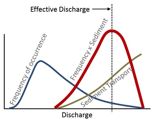
Module 4: Flood and Drought
Module 4: Flood and Drought
In this module, we will discuss the causes, implications and ways to characterize and predict what are often referred to as ‘extreme events’ in hydrology: floods and droughts. Such events play important roles in natural ecosystems and are a major concern for society, with significant impacts on the economy, ecosystem health and services, as well as human health. To gain a broader perspective, we will discuss floods and droughts within the more general topic of hydrologic variability. We will look beyond simple metrics like average annual rainfall to instead think about the full distribution of ‘events’ that characterize the hydrology of an area. The goals of this module are to expose you to the basic concepts of floods and droughts, develop an understanding of how we characterize ‘normal’ and ‘extreme’ hydrologic events, and gain some perspective on the consequences of floods and droughts for society and ecosystems. As part of this, you will become familiar with terms such as stationary versus non-stationary conditions, return period (a.k.a., recurrence interval), exceedance probability, and probability density function.
Goals and Objectives
Goals and Objectives
Goals
- Describe the two-way relationship between water resources and human society
- Explain the distribution and dynamics of water at the surface and in the subsurface of the Earth
- Synthesize data and information from multiple reliable sources
- Communicate scientific information in terms that can be understood by the general public
- Interpret graphical representations of scientific data
Learning Objectives
In completing this module, you will:
- Distinguish between a forecast and a prediction and provide examples of each
- Interpret flood frequency patterns from a histogram
- Interpret flood risk at various locations using flood risk maps
- Explain the hazards of living in a floodplain and the utility of floodways
- Assess flood risk and flood history in your own hometown
- Articulate the concept of a 2, 10 and 100-year flood
Making Sense of Hydrologic Variability
Making Sense of Hydrologic Variability
Video: Advanced Hydrologic Prediction Service (1:37)
This short video introduces the NWS Advanced Hydrologic Prediction Service that provides alerts for droughts and floods in the United States.
Montra Lockwood - Forecaster, National Weather Service, Lake Charles, LA: Floods are one of nature's deadliest natural disasters. Timely and accurate forecasting of floods is vital to the protection of life and property. The Advanced Hydrologic Prediction Service, also known as AHPS, was created for this purpose.
AHPS is a national weather service program designed to provide improved river and flood forecasting. This service provides a suite of text and graphical products that are available online to assist the public, community officials, and emergency managers, in making better life and cost-saving decisions about evacuations and protection of property before flooding occurs. AHPS provides detailed and accurate answers to such questions as, How high will the river rise? When will the river crest? Where will it flood? How long will the flood last? How certain is the forecast? and What are the impacts of the flood? Additional enhancements to the AHPS pages include multi-sensor precipitation information and flood inundation maps for specific locations. To view AHPS information, please visit the AHPS website at water.weather.gov/AHPS. And for more information on flooding and what you can do to protect yourself and your property, visit the National Weather Service's Flood Safety page at nws.noaa.gov/floodsafety.
Precipitation and streamflow are both incredibly variable aspects of the environment, often changing dramatically over short time scales and small spatial scales. If you look up the precipitation record for a location of interest (data freely available from the National Weather Service, Natural Resource Conservation Service, and many other outlets), you would see that events seem to happen ‘randomly’, often without an obvious pattern in the frequency, magnitude or duration. Take, for example, the precipitation record for Kingston, New York from October 1, 2010, through September 30, 2013 (Figure 1). There is an immense amount of variability from day to day. So what can we really say about precipitation from these data? July and August of 2011 appear to be a very wet time period, with many events clustered and one event reaching over 12 cm (nearly 5 inches)! Do you think that caused a flood? Precipitation was very sparse from mid-December 2011 to mid-February 2012. Do you think that was a drought?
It is essentially impossible to answer the questions posed above about July 2011 being a flood or winter 2011-2012 being a drought from the precipitation data alone because precipitation is not the only factor that causes floods and droughts. Processes of water use and transport occurring in a landscape also matter. For example, an increased impervious surface associated with urbanization is known to dramatically increase runoff, resulting in much higher peak discharge (bigger floods) for any given amount of rainfall. In contrast, a large rain event occurring on dry soil will have a relatively small effect on streamflow compared with the same rainfall event occurring on very wet or saturated soils, because more of the rain would be absorbed by the dry soil. Landscape processes also influence droughts. While a prolonged lack of precipitation can initiate a drought, the severity of the drought is strongly influenced by the water demand, by vegetation and/or humans, throughout the landscape. Landscape processes can amplify or dampen precipitation variability. This greatly complicates the job of forecasting floods and droughts. Hydrologists must account for numerous factors that vary in time and/or space.
Though it is difficult, hydrologists can make remarkably accurate and timely predictions of floods and droughts. For example, the National Weather Service (NWS) uses large amounts of real-time data from precipitation gauges, radar systems, river discharge gages, and satellite imagery. The NWS maintains a network of 13 river forecast centers and 50 hydrologic service areas that provide real-time flood warnings throughout the US, which can greatly reduce loss of life and property damages.

| Date | Daily Precipitation (cm) |
|---|---|
| October 1, 2010 | 3 |
| April 1, 2011 | 2.25 |
| October 1, 2011 | 5 |
| April 1, 2012 | 1.5 |
| October 1, 2012 | 3.75 |
| April 1, 2013 | 7.5 |
Forecasting and Predictions
Forecasting and Predictions
Meteorologists have made excellent progress in the past few decades to improve our abilities to forecast when rain events might occur over the next week or so, which facilitates the short-term forecasting of floods and droughts discussed in the paragraph above. However, complex atmospheric dynamics prevent forecasts beyond more than a few weeks in advance. Nevertheless, we must have some basis for making decisions about development, infrastructure and agriculture (e.g., How big should we build a culvert under a road? What size retention basin is needed next to a new housing development? Which agricultural fields will require artificial drainage and which will require irrigation?).
For these longer-term predictions we can use statistics to determine how likely it is that a given location will experience, for example, more than 10 cm of rain in a day, or less than 5 cm of rain during a given month. Many million- and billion-dollar decisions about development and infrastructure are based on such predictions.
To make these predictions, hydrologists synthesize historical data and use a statistics-based approach to determine the likelihood that a given event might occur. While Figure 1 highlights the ‘messiness’ of precipitation events over time, reorganization of the data provides useful information. Figure 2 shows a histogram of the precipitation data presented in Figure 1. A histogram is a plot showing the number of events that fall within chosen data groups or “bins” (shown on the x axis). From these data you can quickly determine that Kingston, NY experiences no rain about 2 out of every 3 days (731 out of the total 1096 days in this record). Only 10 days in the record had rainfall that exceeded 6 cm, so from these data alone you would expect such large rainfall events to happen 10 days out of 1096, or about 1% of the time. On 210 days during this time period the amount of rainfall was between the minimum measurable (typically 0.025 cm or 0.01 inch) and 1 cm (0.4 inches).
Hydrologists tend to use the term ‘forecast’ when referring to a future projection for which we have a lot of information (and therefore relatively high certainty of when an event might occur and what magnitude it might be). In contrast, hydrologists use the term ‘prediction’ for future projections for which less information is available, and therefore uncertainty is greater.

| Daily Precipitation (cm) | Number of events |
|---|---|
| 0 | 731 |
| 0-1 | 210 |
| 1-2 | 70 |
| 2-3 | 43 |
| 3-4 | 14 |
| 4-5 | 8 |
| 5-6 | 10 |
| 6-7 | 2 |
| 7-8 | 3 |
| 8-9 | 2 |
| 9-10 | 1 |
| 10-11 | 1 |
| 11-12 | 0 |
| >12 | 1 |
Learning Checkpoint
The National Weather Service maintains a Precipitation Frequency Data Server (PFDS) website [41] that allows you to look up the frequency of precipitation events of different duration and magnitude for most locations in the US. The PFDS website will open in a new window. Peruse the website and answer the following questions:
Zoom in on Logan, Utah and place the red crosshair directly over Logan. Below the map a table will appear showing the amount of precipitation associated with a range of time periods (durations shown in left column, ranging from 5 minutes to 60 days) and the average frequency with which such an event might happen (the recurrence interval, listed in years).
1. What is the amount of precipitation that you would expect to get in Logan, Utah on an annual basis, within a 24 hour time period?
(a) 0.1 inches
(b) 0.7 inches
(c) 1.2 inches
(d) 2.4 inches
ANSWER: (c) 1.2 inches
2. What is the amount of precipitation that you would expect to get in Logan, Utah on an annual basis, within a 60 minute time period with a frequency of once every 10 years?
(a) 0.1 inches
(b) 0.7 inches
(c) 1.2 inches
(d) 2.4 inches
ANSWER: (b) 0.7 inches
Zoom in on Chickamauga, Georgia and answer the following questions.
(a) 0.1 inches
(b) 1.3 inches
(c) 2.1 inches
(d) 3.3 inches
ANSWER: (d) 3.3 inches
4. What is the amount of precipitation that you would expect to get in Chickamauga on an annual basis, within a 60 minute time period with a frequency of once every 10 years?
(a) 0.1 inches
(b) 1.3 inches
(c) 2.1 inches
(d) 3.3 inches
ANSWER: (c) 2.1 inches
Predicting Frequency and Magnitude
Predicting Frequency and Magnitude
We can do similar calculations to estimate the frequency and magnitude of floods. For example, Figure 3 shows the annual maximum series of flows for the Lehigh River at Bethlehem, PA from 1910 to 2013. The annual maximum series is simply the highest flow value recorded for each year (typically for the water year, October 1 – September 30 as discussed in module 3). The largest flow on record (92,000 cfs) occurred in 1942 (on May 23, to be exact). Note that these are daily flow values which average flow over the course of the entire day, so the actual peak that occurred on May 23 was probably slightly higher. Interestingly, the year that had the smallest peak discharge on record was April 6, 1941 (only 8210 cfs, less than 10% of the whopper flood that came through the following year). But note that we are still talking about the highest flow for that particular year, which is still considerably higher than the average annual flow which is about 1,300 cfs. How can we use this information to predict what might happen in the future to support decisions about development, flood risk, or factors that may influence biota in the river or floodplain (e.g., factors limiting the return of certain fish)?
Similar to the precipitation example above, it helps to reorganize the data. The histogram shown in Figure 4 illustrates the frequency of events in 19 different “bins”. For example, the Lehigh River at Bethlehem, PA has never experienced an annual peak flow less than 5,000 cfs, so there is no orange bar in that bin. But it has experienced 4 peak flows that fall between 5,000 and 10,000 cfs. It has experienced a total of 55 peak flows that fall within the range of 10,000 to 25,000 cfs. These are the most common peak flows for the Lehigh River. And you can see the two outliers at the high end (92,000 cfs in 1942 and 91,300 cfs in 1955).
Typically, hydrologists will approximate the distribution of events that you see in Figure 4 as a probability density function, represented by the smooth, dashed-grey curve superimposed on the plot. This allows them to integrate under the curve above a value of interest to determine the probability that a flood of that magnitude (or larger) will occur. For example, integrating to find the area under the grey dashed curve above 60,000 cfs in Figure 4 would tell you the probability in any given year (in the future) that a flood of that magnitude (or larger) will occur. From that information, you can build your bridge to the appropriate size, or set your flood insurance rates accordingly, etc. Calculating probabilities associated with floods of a given magnitude is discussed in greater detail in the exercise associated with this module.
The same general principles apply to studying droughts. However, as we discuss below, droughts are more difficult to define and quantify because they build up over time and vary immensely over any given area. Nevertheless, similar plots of drought frequency, severity and duration can be developed for droughts, similar to Figure 4, to make sense of all the messy variability we observe in water deficiencies. With this brief introduction hopefully you can appreciate the great challenges in predicting the occurrence and severity of floods and droughts, and you can begin to see the implications for socio-economic systems and ecosystems.


Normal Versus Extreme Hydrologic Events
Normal Versus Extreme Hydrologic Events
The immense variability observed in precipitation and streamflow leads one to wonder what constitutes an ‘extreme’ event. For example, most rivers tend to flood (i.e., water completely fills the channel and spills out onto adjacent floodplain) every one to five years. River discharge during such events is often on the order of 10 times the mean annual flow and often 100 to 1000 times greater than the lowest flows. In that context, perhaps they are extreme. However, considering them within the context of all the floods that occur over a century, we refer to floods that occur every one to five years as ‘common floods’ (e.g., all the events below ~ 25,000 cfs for the Lehigh River in Figure 4 shown earlier). So, labeling an event as ‘extreme’ requires some timescale context. Similarly, what we consider ‘extreme’ varies from place to place. For example, a rainfall event that delivers 5 cm of precipitation is quite rare in Utah but is nearly a daily occurrence in parts of Hawaii.
While there is no formal, universal definition for what hydrologists consider to be ‘extreme’ events, there are numerous ways we can assess precipitation and streamflow events within the appropriate context (timescale and location) to determine how they compare with ‘normal’ conditions.
Notice that the distribution of flood events in Figure 4 (on a previous page) has a strong right (also called positive) skew, meaning a long tail to the right of the graph. This positive skew is common in flood frequency data. It is tempting to label the two events that exceed 90,000 cfs as extreme events, but for many rivers there is no clear cut-off. Instead, hydrologists commonly determine the rarity of an event by calculating the frequency with which the event has occurred in the past. They use that frequency as an estimate of the probability that it will occur in the future, as discussed in the example of the Lehigh River. This is useful way to make predictions, but note that climate change prevents us from using the past to predict the future. If the entire event distribution shifts due to climate change, the event probabilities also change. We will address this issue towards the end of the module.
In any case, terms like ‘extreme’ may be useful for news headlines and catchy titles for scientific presentations, but nature doesn’t easily fit into boxes like ‘extreme’ and ‘normal’. Instead, hydrologists tend to use more well-defined terminology to characterize hydrologic events according to their frequency, duration, and magnitude as well as the spatial extent. Events that occur infrequently (i.e., events of low probability) are the ones to watch out for!
Floods
Floods
Video: Floods 101 | National Geographic (3:27)
This brief video from National Geographic describes the basics of flooding.
Narrator: Over the past hundred years, no other natural disaster in the US has caused more death and destruction than floods. They can happen any place, any day, any time. And they will likely only get worse. As people cluster around coastal regions and flood plains, our growing population will confront the awesome power of water. For thousands of years, farmers have depended on seasonal floods. The waters irrigated their crops and fertilized their lands. Today, excess water is channeled into reservoirs and power hydroelectric dams. But when water levels rise suddenly, far more than the ground can absorb, a flood occurs. Flash floods are a perfect example. Sudden storms unleash a torrential downpour. The runoff moves with surprising force. At a depth of two feet, the water can push aside a car. In fact, half of all deaths from flash floods involve vehicles. But floods occur in many other ways. Heavy rains and thawing snow fall can overwhelm rivers. Storm surge is caused by hurricanes and tsunamis inundate the coastline. Landslides and mudflows can displace large volumes of water. Dams break, levees fail.
In the Great Mississippi Flood of 1993, several of these factors came into play. Over 10,000 square miles of the midwestern United States were overwhelmed with rain. In a cruel twist, the earthen dams known as levees. along the Upper Mississippi River, forced the water to flow downstream faster and stronger. Communities further downriver were hit with the full brunt of the Mississippi. Two-thirds of all the levees were breached. Though towns rallied to protect their lives and livelihoods, the damage was still immense. Over ten billion dollars in damages, 56,000 homes flooded or destroyed, and some 50 people were killed.
At the start of this century, another powerful flood wreaked havoc, this one coming from the sea. The storm surges of Hurricane Katrina submerged 80% of the city of New Orleans. Over 1,800 people died in the floods. The damage has been estimated at over eighty billion dollars. In some ways, the New Orleans disaster was unique. Much of the city lies below sea level and despite years of warning, the city was woefully unprepared to handle a breach of the levees which kept it dry. But we are still vulnerable. Sea levels may rise, coastlines could erode, rain patterns might change, snowpacks could melt, and then the waters would rush in.
Floods are rare events in which a body of water temporarily covers land that is normally dry. Following from module 3, we will mostly restrict our discussion to floods in rivers, but it is important to note that floods also occur around lakes, wetlands, and the sea coast. Indeed, coastal storm surge is among the most dangerous natural disasters expected to result from global warming and sea level rise. River floods occur naturally and in many cases are beneficial for ecosystem functioning because they allow the river to exchange water, sediment, and nutrients with the floodplain and cause scour and deposition that provides habitat for a wide range of aquatic and riparian organisms. However, floods often threaten human infrastructure and livelihoods and can cause severe economic damages.
River floods are typically caused by excessive rainfall and/or sudden melting of snow and ice. Most rivers overflow their banks with small floods about once every two years. Such are the floods that tend to determine the width and depth of a river channel, as discussed in module 3. Moderate floods might occur once every five to ten years and very large floods might only occur once in fifty or a hundred years. The average time period over which a flood of a particular magnitude occurs is called that flood’s recurrence interval, or return period. For example, the very large flood that only occurs, on average, once in a hundred years has a 100-year recurrence interval and is therefore called the 100-year flood. Relating this notion of recurrence interval to the section on probability, above, the recurrence interval is simply the reciprocal of the probability associated with an event (i.e., T = 1/p, where T is the recurrence interval and p is the probability that such an event will occur (or be exceeded), as computed by integrating under the dashed line shown in Figure 4, above the event magnitude of interest). The probability of a 100-year event occurring in any given year is 0.01, or 1%.
We should pay careful attention to our terms here. Note that we are talking about the average time period expected between events. Just because a 100-year event happened last year, there is nothing that says it cannot happen again this year. In fact, the probability of two 100 year floods occurring in back-to-back years is 0.01 times 0.01, or 0.0001. This suggests that, if everything stays the same, the 100-year event should happen in back-to-back years about once every 10,000 years. Of course, over 10,000 year time periods most things don’t stay the same. We’ll discuss this issue, termed non-stationarity, towards the end of the module.
Flash floods are typically caused by heavy rains falling on soils that are already wet or frozen (and therefore have limited capacity to absorb more water), or on land that is covered by snow (in which case the frozen soil has limited capacity to absorb water and the situation is compounded by the fact that melting snow adds to the runoff). Flash floods allow very little time for people downstream to be warned and are therefore especially dangerous. For example, in April 2024, Rio Grand du Sol, Brazil experienced over 30 inches of rainfall over two weeks leading to 150 deaths, 500,000 people displaced from their homes, and over $10 billion in damages.

Expansion of urban areas can increase the frequency, magnitude, and flashiness of floods. Impervious surfaces (roads, parking lots, and buildings) route precipitation directly to stream channels and prevent draining of water slowly through soils to groundwater (Figure 5). The term flashiness refers to the rate at which the water levels rise and fall with faster rising and falling water levels considered flashier.

Hydrologic Versus Hydro-Geomorphic Perspectives
Hydrologic Versus Hydro-Geomorphic Perspectives
Scientists tend to think about floods in two different (but related) ways, one being strictly hydrologic and the other requiring an evaluation of the floodplain topography and how different flow regimes might impact the channel and surrounding areas. In module 3, we explored how hydrologic analyses (analyzing the patterns such as the frequency, duration, and magnitude of flood events) could be used to characterize the river flow regime (e.g., how often does the river exceed 800,000 cfs?). However, a hydrologic analysis does not provide information about the extent or duration of flooding across the landscape (e.g., which parts of the natural floodplain or streets will be flooded?). To predict how much of the floodplain might be inundated by a given flow, we need to consider the channel and floodplain topography (a hydro-geomorphic analysis). For example, a river system with low channel banks and a broad, flat floodplain will experience more frequent flooding of greater extent than a river system with tall banks and a narrow floodplain, given the same flow regime.
Because the size of a river channel can change over time, the relationship between the hydrologic flood frequency and hydro-geomorphic mapping of the area inundated may also change, as discussed in the later module section on hydrologic non-stationarity. For example, the Minnesota River (a major tributary of the Mississippi River) has widened by nearly 50% in the past 3-4 decades. Therefore a flood that may have inundated a significant amount of floodplain 50 years ago may now be entirely conveyed within the channel itself. Thinking back to the example of the Lehigh River in Figures 4 and 5 it is very likely that the 1941 flood (the lowest on record) did not fill the channel and inundate the floodplain. 1943 and 1944 had moderately high peak flows, but may also not have gotten out of the channel because the massive 1942 flood would have widened and deepened the channel. Over the following years, the channel would likely have narrowed again, in response to relatively smaller floods. Flood frequency analysis discussed below and in the exercise associated with this module, is strictly a hydrologic analysis. A hydro-geomorphic analysis is needed to estimate the risk of flood damage. Both types of analyses may be important for engineering plans and ecological studies. High-resolution topography data (elevation data with a vertical precision of about 15 cm and horizontal resolution of about 1 m, also known as ‘lidar’ for Light Detection and Ranging) is revolutionizing the way we make flood inundation predictions. Lidar data contains very detailed information about the ground surface, as well as vegetation on the floodplain, which exerts a strong influence on the velocity and depth of the water. Many states are revising their flood risk maps using this new high-resolution data.
Societal and Economic Implications of Floods
Societal and Economic Implications of Floods
Floods are consistently ranked among the most costly natural disasters around the world, with many billions of dollars in damages reported annually. For example, the Centre for Research on the Epidemiology of Disasters International Disaster Database [43] (EM-DAT) reports that floods accounted for four of the ten most deadly natural disasters in 2013, with confirmed global fatalities exceeding 5000 people (EM-DAT, (2023)). The same 2023 report documents $20.4 billion in damages directly related to river floods.
| Event | Country | Number of Deaths |
|---|---|---|
| Earthquake | Turkey | 50,783 |
| Storm Daniel | Libya | 12,352 |
| Earthquake | Syrian Arab Rep | 5,900 |
| Flood | Congo | 2,970 |
| Earthquake | Morocco | 2,948 |
| Earthquake | Afghanistan | 2,445 |
| Flood | India | 1,529 |
| Tropical Storm | Malawi | 1209 |
| Flood | Nigeria | 275 |
| Flood | Yemen | 248 |
| Total | 80,681 |
During late spring and summer of 1993 heavy rains all throughout the Midwestern US resulted in flooding along the upper Mississippi and Missouri river systems. The floods were the most costly in US history, causing about $15 billion in damages and forcing about 75,000 people from their homes. Heavy rains from Tropical Storm Irene in August 2011 caused approximately $10 billion in damages throughout the Caribbean and eastern United States (including flooding Kingston, NY during the wet period indicated in Figure 1). Notably, the numbers of fatalities associated with these extreme events were relatively low (~50 deaths each) due to remarkably accurate flood forecasting, highly effective emergency response systems and regulations that limit development in flood-prone areas.

Rivers that cannot transport their sediment load (sand and gravel) are particularly susceptible to flooding because sediment settles out in the river bed, causing the river channel to become shallower relative to its banks, thus increasing the chances of flooding. The Yellow River in China is one example of such a river. While the Yellow River has played a pivotal role in the Chinese economy for thousands of years, sedimentation has repeatedly caused the river channel bed and banks to actually build up higher than the surrounding floodplain. This is an especially dangerous situation that can cause the river to catastrophically flood, breach its banks, abandon its channel altogether, and ultimately form a new channel elsewhere within the floodplain, a process known as an avulsion. The Yellow River has caused many devastating floods, including a flood in 1332-1333 that killed an estimated 7 million people. Another Yellow River flood in September of 1887 inundated an estimated 130,000 km2 (50,000 square miles, an area approximately the size of Alabama!) and killed an estimated million people. Yet another flood in 1931 is estimated to have killed 1-4 million. Such catastrophic disasters have earned the Yellow River its nickname, ‘China’s Sorrow.’
Humans have made extraordinary efforts to reduce flood damages. In some cases, these efforts involve limiting development in flood-prone areas. In other cases, these efforts involve building structures meant to control the floodwaters. Flood control structures include dams and retention basins that store water and/or building levees, dikes, and floodwalls that attempt to keep floodwaters confined. Some of the most extensive flood control systems in the world include the floodway diversions on the Red River, which runs between Minnesota and the Dakotas and crosses the US-Canada border into Manitoba.
While we typically think of floods as dangerous and costly natural hazards, they can also provide benefits to society. For example, floods naturally deliver fresh, nutrient-rich sediments to their floodplains, which have historically benefited farmers in many places throughout the world. Yearly floods of the Nile River allowed the early Egyptian people to grow crops, which helped them thrive as a civilization for thousands of years. However, the severity of the floods was unpredictable and floods that were too large caused significant damage. Therefore, in the mid-1900s the Egyptians constructed a flood-control dam on the Nile River. The dam eliminated both the risks and benefits of annual flooding and therefore agricultural practices have had to adapt by using irrigation and petroleum-based fertilizers to replace the water and nutrients that are no longer delivered to the floodplain by the river.
Flood control is not always feasible, given the unpredictable nature of these events as well as geographic or economic constraints. Nor is flood control necessarily desirable in many situations, given the potential environmental benefits for the river and floodplain discussed at the beginning of this section and discussed in greater detail towards the end of this section. In such cases, efforts can be made to reduce economic losses from floods. For example, in many places regulations limit the construction of permanent buildings on floodplains. Emergency response programs, such as the National Weather Service and Federal Emergency Management Agency (FEMA) help flood victims by improving methods to warn and evacuate people from flood-prone areas and to provide relief aid. In an alternative approach, communities in Tonle Sap, Cambodia have constructed their houses on floats and stilts to deal with the annual flooding of 8-9 m (26-30 ft) from the Mekong River.

In many places, flood insurance can be purchased to help cover costs associated with residential and commercial flood damages. However, the private insurance industry is somewhat limited because the number of potential claimants far exceeds the number of people who wish to ensure their property against flooding. As a result, the US Congress created the National Flood Insurance Program in 1968. The program is an effort to provide flood insurance to protect homeowners, renters, and business owners as well as an effort to encourage communities to adopt flood risk management policies established by FEMA.
Droughts
Droughts
Video: California's Extreme Drought, Explained (3:33)
This short video from the New York Times describes the economic and environmental impacts of the severe drought that occurred in California in 2014.
Narrator: Right now 100% of California faces severe drought. This is the San Luis Reservoir near Fresno.
Jennifer Morgan, Tour Guide: You're looking at the largest off-stream reservoir in the United States and it should be twice as full at this date and time. Normally you can see the water line where it's eroded on the hills and along the dam. And usually, we fill up every year except when there's a drought and this is the third year of a major drought.
Narrator: Here's what the reservoir looks like when it's full. Currently, it's only at half capacity. So far this year, California's had only 20% of its normal rainfall and the state's snowpack, another crucial water source, is only 18 percent. Here's a satellite picture of the state from January 2013. And this is from January of this year.
Greg Gustafson, Resident, Lake of the Woods, CA: How can you flush your toilets? How can you take a shower? How can you brush your teeth in the morning?
Narrator: The results of this historic drought are already being felt nationwide.
Bill Diedrich, Farmer, Fresno, CA: A grower like myself, fourth-generation, who has so much emotion and so much of his passion tied up in dirt and production and making things grow, this is a heartbreaker.
Narrator: California produces 90% of the nation's tomatoes, 95% of its broccoli, and 99% of its almonds. That's what Bill Dietrich farms here in Fresno County. For the first time ever, the state has stopped providing water to farmers in some areas.
Bill Diedrich: Our water allocation in this area is zero. Apparently, these trees haven't received any water at all this year.
Narrator: California's agricultural output could fall by three and a half billion dollars this year. Costs across the nation are already up, attributed at least partly to the drought, with more increases expected down the line as crop yields come in this fall. The price for a single avocado could jump by 28 percent. The lack of water also means fire. California officials are bracing for a summer that could be the worst ever. A million acres could potentially burn, with costs that could surpass a billion dollars.
President Obama: Weather-related disasters, like droughts, wildfires, storms, floods, are potentially going to be costlier and they're going to be harsher.
Narrator: So how will California escape this cycle of drought? Governor Jerry Brown has called on Californians to lessen water usage by 20%.
Governor Jerry Brown, CA: And I'm calling for a collaborative effort to restrain our water use.
Narrator: But so far there's only been a five percent reduction. There are also much-needed infrastructure improvements. Converting seawater is one highly costly option. There's also the need to expand California's reservoir system, like the San Luis, for more backup during the dry spells.
Jennifer Morgan: It's going to be tough for everyone because of the drought.
Narrator: But for now drought may be the new norm across California.
California Resident: Instead of just using the dishwasher and wasting the water, might as well do it by hand and fill up the bucket and use it for the plants.
The Wall Street Journal reported that California saw record breaking rains in 2023 and 2024 after a decade of severe drought. In just 2014, 2015, and 2022, California had nearly $7 billion in lost revenue and 40,000 lost jobs in the agriculture sector due to severe drought.
How do you know when you’re in a drought?
Identifying an area as ‘in drought’ is different from identifying it as ‘arid’. While the two may seem related, the subtle difference is important. Aridity is defined as the “degree to which a climate lacks effective, life-promoting moisture” (Glossary of Meteorology, American Meteorological Society). Drought, on the other hand, is ‘a prolonged period of abnormally dry conditions.’ Thus, aridity is a quasi-permanent condition (persistent over human timescales), while drought is a temporary condition (which may persist for weeks, years, or in some cases, decades). The Sahara Desert is an arid environment. The Hoh rainforest in western Washington State is a very humid place that occasionally experiences drought.


Droughts tend to be somewhat elusive phenomena, with severity gradually increasing over many days, weeks, months, or even years. The spatial extent of drought is also quite difficult to delineate, due to the spatial variability in precipitation. Therefore, they are much harder to define, monitor, and identify (relative to floods) within the ‘noisy’ background of natural wet and dry cycles. Yet the impacts of drought can be significant on many facets of the economy and environment. All types of drought originate from a deficiency of precipitation from an unusual weather pattern. If the weather pattern persists for a few to several weeks, it is said to be a short-term drought. However, if precipitation remains well below average for several months to years, the drought is considered to be a long-term drought.


Related to the difficulty in defining drought, economic damages related to drought are also difficult to define. But only considering economic damages that can be directly related to drought, it is clear that they too can be costly natural disasters. In 2023, EM-DAT claims 247 deaths worldwide that were directly attributed to drought (1157 is global annual average from 2003-2022), but a total of nearly \$22 million people were significantly affected by drought in 2023 (average is over \$57 million per year from 2003-2022). Damages related directly to drought in 2023 were estimated in excess of \$22 billion (average of nearly \$9 billion per year from 2003-2022). However, these numbers do not include related effects of wildfire and indirect effects of decreased food production, water quality, etc.
| Phenomenona and direction of trend | Likelihood that trend occurred in late 20th century (typically post 1960) | Likelihood of a human contribution to observed trendb | Likelihood of future trends based on projections for 21st century using SRES scenarios |
|---|---|---|---|
| Warmer and fewer cold days and nights over most land areas | Very likelyc | Likelyd | Virtually certaind |
| Warmer and more frequent hot days and nights over most land areas | Very likelye | Likely (nights)d | Virtually certaind |
| Warm spells/heat waves. Frequency increases over most land areas | Likely | More likely than notf | Very likely |
| Heavy precipitation events. Frequency (or portion of total rainfall from heavy falls) increases over most areas | Likely | More likely then notf | Very likely |
| Area affected by drought increases | Likely in many regions since 1970s | More likely than not | Likely |
| Intense tropical cyclone activity increases | Likely in some regions since 1970 | More likely than notf | Likely |
| Increased incidence of extreme high sea level (excludes tsunamisg | Likely | More likely than notf,h | Likelyi |
Table notes:
a See table 3.7 for further details regarding definitions.
b See table TS.4, Box TS.5 and table 9.4.
c Decreased frequency of cold days and nights (coldest 10%).
d Warming of the most extreme days and nights of each year.
e Increased frequency of hot days and nights (hottest 10%).
f Magnitude of anthropogenic contributions not assessed. Attribution for these phenomena based on expert judgment rather than formal attribution studies.
g Extreme high sea level depends on average sea level and on regional weather systems. It is defined here as the highest 1% of hourly values of observed sea level at a station for a given reference period.
h Changes in observed extreme high sea level closely follow the changes in average sea level. {5.5} It is very likely that anthropogenic activity contributed to a rise in average sea level. {9.5}
i In all scenarios, the projected global average sea level at 2100 is higher than in the reference period. {10.6} The effect of changes in regional weather systems on sea level extremes has not been assessed.
There are four different kinds of drought.
- Meteorological drought refers to a deficit in precipitation that is unusually extreme and prolonged. By definition, meteorological drought must be identified relative to the typical precipitation regime of an area and could be defined as some point out on the long-tail of the distribution of, for example, a plot (histogram or probability density function) similar to Figure 4 [45], except with the x-axis indicating the number of consecutive dry days.
- Agricultural drought refers to a deficit in soil moisture that affects plant growth and productivity. While this term is most often used to refer to effects on agricultural crops, all plants can be affected by soil moisture drought. Paleoclimatologists (scientists who study past climate) examine the thickness of tree rings in woody plants to estimate the timing, duration, and severity of past droughts because water-stressed trees form relatively narrow rings in drought conditions.
- Hydrological drought refers to conditions in which stream discharge and/or lake, wetland and water-table elevations decline to unusually low levels.
- Socio-economic or operational drought refers to conditions when water supply is significantly below demand such that water/reservoir management must be altered. Typically, when meteorological drought occurs, the effects cascade sequentially to the other three types of drought. Likewise, when the meteorological drought ends, the effects cascade in the same sequence, first restoring soil moisture, then restoring other hydrological ‘stocks’ within the system, and hopefully restoring the balance between water supply and demand at key water management infrastructure (i.e., reservoirs).
Activate Your Learning
Go to the US Drought Monitor webpage [46] and answer the following questions:
1. Is the place where you live currently in a drought?
2. Looking back through historical maps, when was the last time your home town was in a drought?
ANSWER: The answer to this question will be different for everyone. Write your answers down and be prepared to talk about it with the class if it comes up.
Measuring the Severity of Drought
Measuring the Severity of Drought
Many different indices have been developed over the past several decades to indicate the occurrence and severity of drought. The simplest index relates precipitation amounts during a specific period of time to the historical average during that same time period. For example, precipitation for the month of June 2014 was 15% below the historical average for Wenatchee, Washington. While this statement conveys some useful information, it is not possible to determine whether or not that 15% deficit qualifies for any of the definitions of drought. The number of days with no precipitation is another simple index, but again must be considered in the context of historical data or water demand, and there is no standard definition for what number of days without precipitation would necessarily qualify under any of the four types of drought. Also, if an area receives a very small amount of precipitation (< 0.1 cm) during an otherwise unusually dry time period, a strict interpretation of this index would ‘reset the clock’, but in reality, the severity of the water deficit remains essentially unchanged. Complex phenomena, such as drought, require somewhat complex metrics to be measured in a meaningful way.
The Standardized Precipitation Index (SPI) is a slightly more complex measure of precipitation deficit that compares measured precipitation to the median historical precipitation over multiple timescales, ranging from one month to 24 months. As dry or wet conditions become more severe, SPI becomes more negative or positive, respectively. Several different indices of varying complexity have been developed to assess drought based on both water supply and demand using multiple environmental criteria. The most common index used to define and monitor drought is the Palmer Drought Severity Index (PDSI), which attempts to measure the duration and intensity of long-term, spatially extensive drought, based on precipitation, temperature, and available water content data. PDSI ranges from values exceeding 4.0, which are considered extremely wet, to values below -4.0, which are considered extreme drought (see Figure 12). Weekly maps of PDSI for the entire US (current and historical) can be viewed on the web page maintained by the National Weather Service Climate Prediction Center [47].
Related indices are the Palmer Z Index, which attempts to measure short-term drought on a monthly timescale, the Palmer Crop Moisture Index, which attempts to measure short-term drought and quantify impacts on agricultural productivity, the Palmer Hydrological Drought Index, which attempts to estimate the long-term effects of drought on reservoir levels and groundwater levels. An immense compilation of current and historical drought information for the entire US is freely available on the US Drought Monitor web page [46], maintained by the University of Nebraska National Drought Mitigation Center.
Increasingly, government and industry groups are using ‘cloud seeding’ techniques to induce precipitation and reduce the severity of a drought. One of the potentially limiting steps in the formation of precipitation is the presence of tiny particles (nuclei) on which water can condense and coalesce to form raindrops or ice crystals large enough to begin falling through the air. Cloud seeding is the practice of injecting nucleating agents, such as silver iodide (AgI), into clouds in an attempt to form precipitation. The effectiveness of these approaches is questionable, but under the right conditions, cloud seeding may increase the probability of rain and therefore it is practiced in some semi-arid regions, including the western US. However, questions remain regarding environmental and human health impacts as well as concerns regarding ‘stealing’ atmospheric moisture from would-be recipients downwind.
Learning Checkpoint
1. What was the Palmer Drought Severity Index for the week ending on June 8, 2024, for the following locations (see Figure 12 above):
St. Louis, Missouri
ANSWER: 0
San Antonio, Texas
ANSWER: -2 to -2.9
Boston, Massachusetts
ANSWER: 4
2. Which of these three locations were likely experiencing socio-economic drought during this time, forcing them to actually change water use/management practices, at least temporarily?
San Antonio, Texas
Boston, Massachusetts
Miami, Florida
ANSWER: San Antonio, Texas
Floods and Droughts Impact Ecosystems
Floods and Droughts Impact Ecosystems
How do floods and droughts impact ecosystems?
Variation in river flow (i.e., the river flow regime – see Module 3) exerts a strong influence on river and riparian ecosystem function. In particular, floods and droughts control the creation and maintenance of river and floodplain habitats and the sustainability of the high biodiversity observed along river systems. The temporal pattern of floods interacts with channel and floodplain topography to create a highly heterogeneous landscape of depressions, oxbows, gravel bars, and terraces (Figure 13). The hydro-geomorphic diversity means that the inundation frequency varies strongly over short distances on river floodplains, and creates habitats for a diverse suite of organisms adapted to a wide range of flooding frequencies.

Both riparian and aquatic organisms have adapted to take advantage of flood-drought cycles in river ecosystems. For example, many fish species time spawning runs to coincide with predictable floods, because this allows large adult fish to access small streams that provide optimal habitat for egg development and growth and survival of young fish. In the Amazon River, many fish species can almost be considered forest-dwelling fish, because they feed directly on leaves, fruits, seeds, and insects that fall into the river when it floods surrounding forests during the annual rainy season. Trees of these seasonally flooded forests have in turn developed fruits and seeds that mature during the flooding season and that can survive fish digestive systems in order to take advantage of the seed dispersal ability of mobile fish species. In the western U.S., cottonwood trees time the release of seeds to coincide with the recession of flood peaks in order to access fresh sediment deposits with elevated water tables that provide ideal habitats for germination.
It may be less obvious that droughts could be beneficial for aquatic and riparian biota, but when coupled with periodic flooding, droughts play an important role in the survival of many river organisms. During droughts, resources such as organic material and nutrients can accumulate on floodplain surfaces, and when a flood does occur there is a pulse of greater resource availability than would occur under regular flooding, and this period of high resource availability can ensure the quick growth and survival of organisms, including young fish. In addition, periodic drying of rivers and floodplain wetlands eliminates competitors and predators for organisms that can quickly colonize areas when water returns. Such areas of refuge from predators are critical for the persistence of many aquatic organisms and would not exist without periods of drought.
The importance of floods and droughts to the integrity of river-floodplain ecosystems is apparent when alterations to the natural flow regime occur. Riverine organisms are often closely adapted to the local magnitude, frequency, duration, and predictability of extreme events, such that alteration of any one component can threaten species persistence. For example, recruitment of cottonwood trees along many dammed rivers in the western U.S. has essentially ceased, because the dams prevent flooding and creation of germination sites during the spring when cottonwood trees release their seeds. Excessive drought is also highly detrimental to river systems. One of the most famous examples of drought impacts is seen in the Colorado River delta in Mexico, which was once a highly productive floodplain forest and swamp, but due to prolonged drought conditions in the river basin and water infrastructure development, is now a dry desert.
Hydrologic Variability Versus the Human Need for Water Resource Reliability
Hydrologic Variability Versus the Human Need for Water Resource Reliability
Floods and droughts are natural phenomena throughout the world and natural systems have adapted to this variability over time. But human demands for water resources are not so adaptable to variable hydrologic patterns. What if you could only turn on the tap during and immediately after rainfall events? Hydroelectric dams also require a constant supply of water to respond to electricity demands on timescales of minutes and hours. Farmers in drier areas require a reliable supply of water to keep crops watered and soils from drying out. In response to societal needs for a reliable and sufficient supply of water, we have developed an extensive infrastructure to even-out variability in natural flow regimes and therefore reduce uncertainty associated with both floods and droughts.
In particular, dams and reservoirs have been constructed around the world to store water during times of flood and provide water during times of drought – as discussed in detail in the next module (Module 5) (Figure 14). Over half of the world’s large river systems (those holding 60% of the world river discharge) are impacted by dams. In fact, the construction of dams and associated filling of reservoirs slows the rotation of the Earth (though only adding ~0.1 microseconds to the length of a day)! However, as we will see in Module 5, the construction of dams and evening out of hydrologic patterns has profound impacts on geomorphic and ecological processes in river systems, and the manipulation of discharge leads to reduced variability in flow regime (e.g., Figures 15 and 16), among many other effects.


Non-Stationary Hydrology
Non-Stationary Hydrology
When ‘normal’ changes: non-stationary hydrology
As we have discussed at length above, floods and droughts can have significant impacts on society and the environment. However, as also discussed above, we can characterize the frequency, duration and magnitude of these rare or extreme events and both human and natural systems have mechanisms to deal with them. For example, we can estimate the magnitude of a 100-year flood and build a bridge sufficiently large to pass the flood with minimal risk of damage to the bridge or changes in water depth (i.e., from water backing up behind the bridge and therefore flooding additional land upstream). Similarly, we can compute the width of a floodplain that would be inundated from that 100-year flood and choose to not build within that flood corridor, or choose to require those who do build within the flood corridor to purchase flood insurance to cover costs of potential damages.
Similarly, as we discussed in module 3, river channels naturally adapt their width and depth to accommodate common floods. Thus, society and the environment naturally develop some amount of resiliency to historical climate extremes. However, all of the prediction methods we have discussed so far in this module rely on the assumption that the future will look statistically similar to the past (i.e., the distribution of events will not change and occurrence of events in the future will be consistent with the probabilities computed from the histograms or probability density functions such as those shown in Figures 3 and 4). This assumption is known as the Stationarity Assumption in hydrology. Specifically, stationarity implies that while there is considerable variability in precipitation and streamflow, that variability is bouncing around a relatively constant average value and has a relatively constant spread, as shown in the hypothetical plot of peak streamflow over time in the left panel of Figure 17. From left to right, the mean (µ) and standard deviation (s, i.e., the spread of the data around the mean) don't change. However, as climate changes, the magnitudes, durations, and frequencies of floods and droughts may occur that are outside the historical range of observations, resulting in a change in the average magnitude of floods (Figure 17, middle panel) or a change in the variability of floods (Figure 17, right panel). In either of these situations, the statistics from the left side of the graph don't provide a good basis for making predictions about the right side of the graph (or predicting what will happen in the future!). Understanding and accounting for such non-stationary patterns in precipitation and streamflow are among the greatest challenges in hydrology today because we need to make accurate future predictions for many decisions about flood and drought risk, infrastructure design (roads, bridges, culverts, ditches, parking lots, detention basins, sewers, etc.!) and water availability. So this is a hot topic in the field and many new techniques are emerging!
Non-stationarity will be common in the future as regional climates systematically change. According to the Intergovernmental Panel on Climate Change, climatic warming will increase the risk of both floods and droughts (Table SPM2 in IPCC, 2007; see also IPCC, 2014 and IPCC 2023). The multitude of factors that combine to ultimately cause floods and droughts are exceptionally difficult to predict over the next few decades. Nevertheless, there is a high level of agreement among the competing IPCC climate simulation models regarding the general trends of several metrics. For example, precipitation intensity increases are expected in most places and especially at mid- and high-latitudes where mean precipitation also increases. Summer droughts are also expected to increase over low and mid-latitude continental interiors. Snowpack is expected to decline overall as more precipitation will fall as rain rather than snow, especially in areas with temperatures near 0°C in fall and spring. Relatedly, snowmelt is projected to occur earlier. The combination of less snowpack and earlier snowmelt increases risk of summer to fall drought in snowmelt dependent regions, such as the western US. Some regions outside the US are highly dependent on meltwater from glaciers for water supply. Accelerated melting due to climatic warming increases the risk of flooding downstream in the near-term. In the long-term, glaciers in many of these areas will shrink and ultimately cease to exist, posing a serious threat to the downstream water supply. This poses a serious risk to the hundreds of millions of people in China and India who depend on glacial meltwater from the Hindu Kush-Himalayas. In closing, there is a good reason to expect floods and droughts to become more severe in the coming decades, increasing the urgency for improved predictions, mitigation efforts, and adaptation strategies.
Module 5: Dam it All!
Module 5: Dam it All!
Introduction
In the preceding modules, we’ve discussed the uneven distribution of precipitation and water resources on Earth’s surface (Modules 1-2), and the dynamics of rivers and streams as the primary conduits for the return of water that falls over the continents to the oceans (Modules 3-4). One fundamental challenge to populations is that precipitation does not fall where we need it when we need it. This is amplified by the fact that many population centers are located in areas that are perennially dry, including those in the US Southwest.
How do we store water delivered by rivers to provide reliable and secure supply when we need it, where we need it, and tame the flow in abnormally wet conditions to mitigate flooding? The main solution is to dam rivers and fill the reservoirs behind them. This stores large volumes of water that ensure a stable supply, the reservoirs act as “capacitors” in the hydrologic system to absorb excess flow and thus prevent flooding downstream, and the dams simultaneously produce electric power as water is released in a steady, controlled discharge from the reservoir. However, dams and their reservoirs also profoundly impact the natural river system and can cause irreversible changes to the environment and to populations both near the dam and far up- and down-stream. In Module 5, we will explore the benefits and consequences of construction and removal of large dams, both in the US and globally, including a discussion of case studies along the Yangtze and Nile rivers.
Goals and Objectives
Goals and Objectives
Goals
- Describe the two-way relationship between water resources and human society
- Explain the distribution and dynamics of water at the surface and in the subsurface of the Earth
- Synthesize data and information from multiple reliable sources
- Identify strategies and best practices to decrease water stress and increase water quality
- Thoughtfully evaluate information and policy statements regarding the current and future predicted state of water resources
- Communicate scientific information in terms that can be understood by the general public
Learning Objectives
In completing this module, you will:
- Weigh the advantages and drawbacks of large dams, including economic, environmental, and cultural impacts
- Explain the reasons why dams are built, and the rationale for removing them
- Assess whether government agencies should be responsible for regulating new dam construction
- Debate whether a dam is the most appropriate solution to water needs and flood control in a particular location
Introduction to Dams
Introduction to Dams
Think about your impressions of dams and the reservoirs behind them that you have seen. Large concrete dams have grandeur, and the huge lakes that they contain are often sited in attractive canyon or valley settings and provide picnic, swimming, and boating facilities. If you had grown up in the arid southwestern U.S., you might have thought of these as oases—providing relief from summer heat and dryness; had you grown up in the eastern U.S., you may have appreciated the dam-impounded reservoirs as camping and fishing spots. It is likely that, when you were young, you did not appreciate the real purposes of these structures or the controversies that surrounded some of them as they were proposed and built.
Dams most importantly provide: 1) dependable water supplies in areas experiencing significant annual fluctuations in precipitation and runoff or lacking other water sources such as groundwater; 2) a flood control buffer for times of excessive precipitation and runoff; 3) hydraulic head for generating hydroelectric power; and 4) recreational opportunities including boating, fishing, and swimming. During the colonial settlement and expansion in eastern North America, dams provided direct hydropower primarily for mills. Later, during the settlement of the semiarid to arid west, small dams provided water storage for irrigation and watering livestock. These two contrasting uses of dams, one in a relatively water-rich region, and the other in arid lands led to different water laws, which have been outlined in Module 1. An estimated 75,000 dams (over 25 feet) have been constructed in the U.S. alone (Graf, 1999), providing water storage of about 4 acre-feet (5000 m3) per year per person. Please go to this video of U.S. dam building since the early 1800s to see the pace and geographic location of dam building.
Video: US dams (00:20) This video is not narrated.
If the video does not play, watch it on the CSDMS website [49].
Figure 1 illustrates the increase in water storage from 1900 to the present on a global basis. This compilation shows clearly the impact of the U.S. dam building era, beginning in the 1950s as well as the decrease in the rate of water storage beginning in the 1980s with reduced rates of dam construction and the onset of dam removal projects. With an estimated 22,000 large dams China's push to build more dams is creating controversy.
Reading
Please take some time to read about it China’s Great Dam Boom: A Major Assault on Its Rivers [50].

Activate Your Learning
1. Why are large dams constructed? List four reasons.
ANSWER: Flood prevention, water supply, power, recreation.
2. From inspection of Figure 1, during what time period was dam construction happening most rapidly?
ANSWER: Where the slope of the graph is steepest, reservoir capacity was increasing most rapidly; this is between around 1955-1990.
3. Globally, dam construction has tapered off since around 1990-1995. Can you think of any reasons why this would be the case?
ANSWER: There are probably several reasons. For the most part, the best and largest dam sites have already been developed. In addition, environmental impacts and concerns have become increasingly visible and led to more opposition and stricter regulation.
Dams are, at times, perceived as being environmentally benign, particularly because the generation of hydroelectric power involves no direct greenhouse gas emissions. But there are impacts of dams that are deleterious to the environment and human health. For example, one of the major impacts of having constructed large dams on active, high gradient river systems carrying large volumes of water and sediment is the buildup of sediment behind the dam(s) and the decrease in sediment supply to coastal regions. Many modern deltaic coasts, including the Mississippi Delta region and the Colorado River Delta in North America, have been receding rapidly as the result of a series of dams emplaced on the Missouri River and the Colorado River, respectively. There are also impacts of ponded waters on human health, particularly in tropical regions where diseases and parasites are harbored by the biota in warm, slowly circulated waters. In addition, dams commonly impede the upstream migration of anadromous fishes to spawn, including shad and herring on the east coast of the U.S. and steelhead and salmon in the west, thus limiting natural populations and reaches of these fishes. Controversy surrounds many older dams that impede fish migration. Dams also alter environmental conditions, including changing water temperatures, oxygen concentrations, and nutrient loads that can substantially alter the ecology of river systems, as can be seen in the case of the Colorado River below Glen Canyon Dam (see below).
Yet, dams do serve human needs and there is a rich history of dam building in the U.S. that has now diminished (Figure 1). Although dams are now rarely constructed in the U.S., other countries have continued to build dams to control floods and provide hydroelectric power. In the U.S. many hydroelectric dams require upgrades and recertification because of newer regulations. Such aging dams, many privately owned, face economic pressures in conforming to modern requirements that include studies of environmental impacts, possible additions of fish ladders that will allow fish to bypass dams, etc. These impacts are weighed against benefits (water storage, hydroelectric power generation) in recertification. Increasingly, dam owners assess costs and find it much less costly to remove a dam than to refit it to conform to requirements. A number of large dams have now been removed or are proposed for removal. Even though dam removal can be beneficial, there are also possible significant environmental issues to be confronted, including the amount and composition of sediment ponded behind the dam.
Ponding the Waters: Impacts of Dams
Ponding the Waters: Impacts of Dams
As we’ve covered in the first part of this module, the need for dams is largely driven by the uneven distribution of precipitation, resulting from river discharge, and thus water supply – in both time and space. Dams control river flows and provide capacitance in the river channel to satisfy demands for continuous water supply (i.e. for irrigation and domestic use, for flood control, and power generation). However, such large-scale alteration of the natural river has wide-ranging impacts both upstream and downstream, where the ecology, geology, hydrology, and human populations have evolved in tandem with undisturbed patterns of variable river discharge. Here we’ll briefly cover some of these impacts, and highlight using examples from well-known case studies including the Three Gorges and Aswan High Dams.
Nutrient Supply to Floodplains
Nutrient Supply to Floodplains
Flooding is a natural process that replenishes soil and nutrients to floodplains. Of course, floodplains are ideal sites for agriculture – they are flat, water is accessible, and – at least prior to modification of the system by levees or dams – the soils are among the most fertile on Earth due to recurring flooding that deposits nutrient-rich fine-grained sediments. Historically, these are the sites of major agricultural and population centers, including the “Fertile Crescent” along the Tigris-Euphrates floodplain (now largely barren due to long-term effects of irrigation-based agriculture and flood prevention), and the Nile Floodplain (see The Nile River and Aswan Dam below). Likewise, most major modern agricultural production is localized to floodplains - including the Central Valley of California, the Susquehanna River Valley, the upper Tigris-Euphrates basin, the Nile Valley, and the floodplains of the Mississippi and Missouri Rivers.
Prevention of flooding through the combination of dams (which control river discharge) and levees (which artificially channelize flow and shunt it downstream so that it cannot spill onto the floodplain) is a strategy to limit the loss of crops and property, and allow development in otherwise flood-prone areas. This approach, while generally effective in limiting short-term losses, affects soil fertility, groundwater systems, and the health of downstream waterways in the longer-term. For example, flood prevention eliminates a major source of recharge to aquifers in valley-fill sediments that lie below the floodplain. Recurring floods also serve to flush salts that accumulate naturally in soils due to evaporation and transpiration (i.e. water is transported to the atmosphere by these processes, but even small amounts of dissolved salts remain in the soil). Reduction or elimination of this flushing can lead to soil salinization, with negative effects on soil fertility.
Perhaps most notably, by eliminating or limiting the replenishment of nutrients to the floodplain, imported fertilizer is required to grow crops. Excess fertilizer application, in turn, leads to runoff enriched in Nitrogen and Phosphates that affects aquatic species and can cause eutrophication of lakes and estuaries downstream. This is a longstanding problem that leads to algal blooms at river mouths, consumption of Oxygen by organic matter (dead algae), and ultimately to “dead zones” in these regions that affect fisheries (Figure 2).

Learning Checkpoint
1. Why are floodplains historically ideal for agriculture? List three reasons.
ANSWER: Nutrient supply, soil replenishment, water supply, typically flat. Could also note that rivers provide transport pathway for produced goods.
2. What is the main negative effect of eliminating the replenishment of nutrients to floodplains on ecosystems and river health downstream?
ANSWER: It leads to the addition of fertilizers and nutrients to the land, which in turn runs off to the river and ultimately the ocean. This leads to algal blooms that extract dissolved oxygen from the water, and cause hypoxic, or “dead” zones that impact fisheries and ecosystem health.
The Nile River and Aswan Dam
The Nile River and Aswan Dam
Large rivers are difficult to control. The Nile River, so important to Egypt's populace, is no exception. But since the late 1960s, the Nile River has been under the control of humans because of the construction of the Aswan High Dam. Part of the rationale for this dam was to manage the natural cycles of flood and drought to produce dependable water supplies for farming and other uses. The consequences of cyclic climate variations on a decadal scale were buffered by the large storage capacity of the Nile Valley behind the High Dam, which is nearly six trillion cubic feet (157 km3) of water! This is about four times the amount of water stored behind Hoover Dam (USA, Lake Mead) and Three Gorges Dam (China) (Chao et al., 2008). In addition, the Aswan High Dam initially produced a significant amount of electrical power (about 50%, now less than 15% of Egypt's needs) that allowed electrification of "rural" Egypt.
Figure 3 shows the narrow Nile River Valley slicing northward through the Egyptian desert. The narrow green band of the Nile River Valley represents farmland irrigated by waters of the Nile River. Prior to the completion of Aswan High Dam, the Nile River would flood its valley annually during the rainy season in its higher altitude headwaters (Ethiopia, Sudan, Kenya, Uganda), bringing nutrient-rich silt to fields and renewing fertility. In addition, a substantial volume of sediment was carried down the Nile River Channel to its large delta, building out the delta into the Mediterranean Sea, providing additional fertile land for farming. This no longer happens because the Aswan High Dam effectively (an unintended consequence) traps sediment carried from the highlands behind it. Now, the delta region, which subsides naturally as the result of compaction of sediment (newly deposited sediments have water contents of 70% or more that are reduced by compaction by overburden), is diminishing in size because rates of coastal erosion exceed supply of sediment. Currently, almost 1/3 of the Nile Delta’s land area sits within a meter of sea level. Subsidence rates vary across the delta, but in some areas, the land surface is sinking as fast as 1 cm/yr. Control of the Nile’s flow has also lead to water quality problems. Because once-regular floods no longer flush salts, sewage, fertilizers, and waste from the delta, surface waters are polluted and those living near the Mediterranean coast increasingly rely on groundwater to meet demand for drinking water and domestic use. Extraction of groundwater, coupled with land subsidence, has led to saltwater intrusion in the aquifer as far as 30 km inland.
There have been other unintended consequences of the Aswan High Dam including the spread of disease (Schistosomiasis), a decrease in water quality and increase in algal blooms resulting from fertilization of farm fields and irrigation runoff, flooding of historical sites, and displacement of people from the regions flooded by the reservoir.
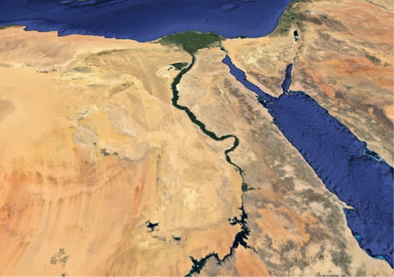
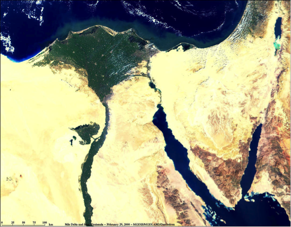
Sediment Trapping
Sediment Trapping
Because large reservoirs behind major dams are areas where water flow velocity is slowed (also often called “slackwater”), sediments are deposited where rivers enter the water body (Figure 5). Sedimentation in reservoirs behind dams has several consequences. Sediment deposition reduces reservoir water storage capacity and therefore limits the useful lifetime of the dam for flood control, water supply, and hydropower generation. Recent detailed studies of storage capacity and sedimentation rates for reservoirs in the U.S. suggest that average annual storage losses range from less than 0.5% to more than 2% (see supplemental reading: Graf et al., 2010; “Sedimentation and sustainability of western American Reservoirs, Water Resources Research”). The highest rates of storage loss are occurring in the American West, and the lowest in the Northeast.
For example, almost 20 million tons of sediment are deposited annually in reservoirs along the Mississippi River (UNESCO, 2011). China’s Three Gorges Dam alone (one of several along the Yangtze River) traps 34 million tons of sediment per year, or 31% of the river’s sediment load (Hu et al., 2009). Globally, the amount of sediment trapped in dams is estimated to be 73 km3 (Syvitsky & Kettner, 2011) and storage loss to trapped sediment has reached 16% of initial storage capacity with an expected 26% loss by 2050 (Perera et al., 2023).This sediment accumulation slowly reduces reservoir capacity behind dams and is one factor that limits their useful life expectancy. Recent studies of sediment accumulation suggest that the life expectancy of Lake Powell is ~300-700 yr, and that of the Three Gorges Reservoir in China is ~150 yr.


The concomitant reduction in sediment delivery to downstream areas also has several consequences (Figures 5-6). Ultimately the decreased sediment supply to the river mouth translates to net erosion of beaches and loss of land in coastal regions, as natural coastal erosion by currents and subsidence caused by compaction of delta sediments is not offset by delivery of sediment. For example, prior to construction of the Aswan High Dam began in 1960, the annual sediment flux to the Nile Delta was ~100 million tons. This sediment supply was enough to offset erosion and natural subsidence.
Consequences of Concomitant Reduction
Consequences of Concomitant Reduction
The concomitant reduction in sediment delivery to downstream areas also has several consequences (Figures 7-9). Ultimately the decreased sediment supply to the river mouth translates to net erosion of beaches and loss of land in coastal regions, as natural coastal erosion by currents and subsidence caused by compaction of delta sediments is not offset by delivery of sediment. For example, prior to construction of the Aswan High Dam began in 1960, the annual sediment flux to the Nile Delta was ~100 million tons. This sediment supply was enough to offset erosion and natural subsidence.

Without continued sediment delivery, subsidence and coastal erosion lead to significant losses of land area (Three Gorges: A “Mega-Dam” and its Impacts), much of which is prized for agriculture or development. Currently, parts of the Nile Delta are subsiding at up to 1 cm/yr. This phenomenon is common to most of the world’s major river systems, including the Mississippi, Colorado, Yangtze, and Indus Rivers (Figure 7). For example, much of New Orleans is subsiding at over a half-centimeter per year, with some areas sinking more than 2.5 cm/yr (Figure 9). The combination of subsidence, coastal erosion, and sea-level rise has led to land loss from the Mississippi Delta of almost 1100 acres per year since the mid-1970s.
The same processes also place these areas at especially high risk for flooding in major storm events. Much of the inundation of the Gulf Coast caused by Hurricane Katrina in 2005 occurred in areas that lie below sea level due to subsidence. The effects of subsidence are compounded by the loss of barrier islands as their sediment supply is not replenished. Further, extraction of groundwater from the subsurface – and in some cases oil and gas - exacerbates land subsidence, and can also lead to saltwater intrusion in coastal aquifers.


Consequences of Release of Water
Consequences of Release of Water
Release of water from the downstream side of reservoirs at dams affects the ecology of the river downstream because there is little or no entrained sediment to replenish alluvial deposits along the river, and, in fact, the now sediment-starved river is more likely to erode existing bars, beaches, and riverbeds. In many cases, the clear water released from dams can erode fine-grained sediments (silts and clays) from river banks and bars, leaving behind the coarser sand and gravel deposits that would require higher flow velocities to mobilize (as we covered in Module 3…remember?). Increased scouring can also lead to destabilization and landsliding along the river banks.
Erosion of sandbars and beaches poses a threat to native fish species that depend on sheltered waters for spawning or their fry. For example, the population of the humpback chub, a fish species native to the Colorado River system, has decreased by an estimated 75% since 1982. The chub was uniquely adapted to thrive in the sediment-laden, low-visibility and naturally turbulent waters of the Colorado River. Since the construction of Glen Canyon Dam, the clear, colder, and more stable flow has favored non-native predatory species like brown and rainbow trout.
Deposition and storage of sediments behind dams also lead to the buildup of organic material and nutrients adsorbed to sediment grains or trapped in pore spaces that will be released if the dam is decommissioned. As discussed in the next part of this module (“Bringing Down the Dams”), if or when dams are decommissioned, many years’ worth of sediment, nutrients, and carbon must be managed. Release of the stored sediment can lead to:
- inundation of the river system with suspended sediment that increases water turbidity
- introduction of nutrients to the river mouth that can lead to eutrophication and dead zones
- the potential release of toxins, including metals and volatile organic compounds adsorbed to fine sediment, to downstream areas

Recent controlled water releases have been conducted to explore the possibility of delta and downstream habitat renewal. In 1996, a seven-day-long experimental release of 1290 m3/s (that’s about 20 million gallons per minute) from Glen Canyon Dam was conducted to evaluate the prospects for the restoration of stream habitat through the rebuilding of sandbars and beaches. The experiment yielded mixed results – most notably that sand was initially deposited on bars and beaches, but only during the first couple of days of the release. There was not enough sediment load in the released water to sustain deposition, partly because the experiment was not synchronized with the natural seasonal sediment flux from upstream tributaries; as a result, existing bars were eroded and remobilized in the late stages of the controlled flood. In March 2014, a “pulse flow” of 105,000 acre-feet (about 1% of the River’s annual discharge) lasting until mid-May was released from Morelos Dam to bring water to the Colorado River Delta through a joint US-Mexico initiative. You can listen to a brief news story about the experiment: Well, I'll be Un-Dammed: Colorado River (Briefly) Reached The Sea [54]. The pulse flow was designed to mimic natural spring floods that disperse seeds, nourish the delta, and provide habitat for waterfowl. These experiments suggest that partial restoration may be possible, but will likely require a better understanding of the dynamics of stream habitats and sediment delivery and transport processes.
Other Impacts
Other Impacts
In this section, we will consider other impacts of dams.
Pollution
Pollution
In addition to the increased nutrient concentrations from agricultural return flow downstream of dams, the reduction in flow velocity in slackwater behind dams leads to reduced flushing of pollutants that enter the river. In areas subject to high rates of municipal or industrial wastewater discharge, or to agricultural runoff, this can lead to significant impairment of water quality in the reservoir itself, and in upstream tributaries (for example, see Three Gorges: A “Mega-Dam” and its Impacts). High nutrient fluxes can also lead to eutrophication of the reservoir. Additionally, the increased surface area of reservoirs leads to large evaporative losses and subsequent increases in water salinity, especially in arid and semi-arid climates.
Fish Spawning and Migration
Fish Spawning and Migration
As noted previously, dams have wide-ranging effects on downstream habitat through changes they cause to water turbidity and sedimentation and erosion patterns. These changes threaten certain species that have evolved to thrive in the natural system – like the humpback chub – through a combination of decreased or degraded breeding habitat and increased predation by non-native species. Additionally, because water released from dams through intakes flows from the deep part of the reservoir, it is commonly colder than the natural river flow – and its temperature is less variable than in the river’s natural state. For example, prior to construction of the Glen Canyon Dam, water temperature in the Colorado River varied from ~0 to 27° C over the course of the year; water discharged from the dam now averages ~8°C and varies little seasonally. The changes in water temperature and its variability impact some fish species, which rely on temperature cues to trigger key lifecycle events. The lower oxygen levels in waters released from storage behind dams also impact fish downstream.
Finally, dams present physical barriers to catadromous and anadromous fish species (those that spawn in saltwater and live in freshwater, and vice-versa, respectively). These fish migrate either upriver from the ocean (anadromous), or downriver to the ocean (catadromous) to spawn. After hatching, the young fish migrate in the opposite direction. Of these, perhaps the best known is the salmon, which migrates up-river to spawn, commonly over hundreds or thousands of km – for example, although greatly reduced due to major dams along the Columbia and Snake Rivers, Chinook salmon runs commonly extend from the Pacific Ocean all the way to Idaho! Structures designed to allow fish to navigate dams, such as fish ladders, are one solution, but they still present a barrier that reduces the likelihood of safe passage, and thus fish numbers.
Diseases – A Tropical Malady
Diseases – A Tropical Malady
The large reservoirs impounded by dams provide breeding grounds for some water-borne diseases and parasites, especially in tropical climates. Among the most prevalent of these is schistosomiasis, a disease caused by parasitic worms. The parasite is spread by freshwater snails, and has come to be known as the “disease of hydroelectric dams”. It infects an estimated 200 million people per year (with 200,000 fatalities), primarily in Asia, Africa, and South America. Through the expansion of habitat for the disease vector by large slackwater reservoirs, the incidence of this and other diseases is greatly increased. For example, in the Yangtze River Basin, the incidence of schistosomiasis is near 5%, versus less than 1% in less or undeveloped areas.
Dams and major irrigation projects also provide expanded breeding habitat for insects (mosquitos) that serve as vectors of Dengue fever, malaria, and West Nile virus, among others. The World Health Organization (WHO) estimates that malaria cases in villages near the Bargi reservoir in India increased more than twofold following the dam’s construction, and up to four-fold in villages closest to the dam itself. Likewise, malaria incidence increased by seven times in proximal Ethiopian villages following the construction of small dams on the Tigray River. A similar increased incidence of West Nile virus has been documented as a result of increased mosquito breeding area in many parts of the world, including the Midwestern U.S., California, and Oregon.
Earthquakes and Structural Failures
Earthquakes and Structural Failures
Impoundment of water behind major dams changes the distribution of stress in the Earth’s crust, and in combination with downward percolation of impounded water, can trigger seismicity. For the most part, this phenomenon is restricted to increased numbers of small (magnitude <3.5) earthquakes triggered by the increased load of millions of m3 of water, associated warping – or flexure – of the crust, and diffusion of water pressure from the reservoir along fractures and fault lines (Figure 10). Although hotly debated, reservoir-induced seismicity has even been invoked as a possible mechanism for the devastating 2008 magnitude 7.9 Wenchuan earthquake that killed an estimated 80,000 people (see one news article discussing this issue here [55]). The reservoir impounded behind the 156 m-tall Zipingpu Dam lies above the Beichuan- Yinxiu fault, which extends to the Northeast to the earthquake hypocenter, located ~50 km away.
Although remote, there is also a potential risk of dam failure to life and property downstream. In some cases, the causes of such failures are not known with much certainty. For example, the collapse of the St. Francis Dam Northeast of Los Angeles in 1928 resulted in the catastrophic release of over 12 billion gallons of water. The flood wave, which was over 140 feet high, killed an estimated 600 people and scoured the valley below, transporting fragments of the dam as large as 10,000 tons for almost a mile downstream. In other cases, upstream flooding or inadequate ability to release water and relieve pressure on the dam are the culprit, as in the famous collapse of the South Fork dam and resulting 1889 Johnstown PA flood that killed over 2000 people and triggered changes to liability laws in the U.S. In 1986, a similar disaster at the Glen Canyon Dam was narrowly avoided.

Politics and Control of Flow Across Borders
Politics and Control of Flow Across Borders
Rivers are not restricted by state and national borders, whereas dams are rarely constructed or managed by collaboration between governments. As a result, alteration, interruption, and control of river discharge by dams naturally leads to political and legal conflict. In the case of the Colorado River, which we will cover in more detail in Module 8 (Cities in Peril), the allocation of water between states within the drainage basin is governed by the 1922 Colorado River Compact. Allocation of water between the U.S. and Mexico is governed by an international treaty established in 1944 and revised in 2012. Even though well established, the water allocation of the Colorado, and its fairness are widely debated. The compact is also the focus of lawsuits over water rights for Native American reservations, which were not explicitly included in the original agreement. Court battles have also arisen over other river flows in recent years (for example in Florida and Georgia, and along the San Joaquin and Sacramento Rivers) pitting access for communities or farmers against minimum limits on flow required to support endangered species.
Globally, other rivers and dams are the source of equal – or more – controversy. As one example, at the 1992 opening ceremonies for the Atatürk Dam on the Euphrates River in Turkey, the president of Turkey is reported to have said, "Neither Syria nor Iraq can lay claim to Turkey’s rivers any more than Ankara could claim their oil. This is a matter of sovereignty. We have a right to do anything we like. The water resources are Turkey’s, the oil resources are theirs. We don’t say we share their oil resources, and they can’t say they share our water resources." The conflict over waters of the Tigris-Euphrates continues (you can listen to a story about this dispute here [56]). Dams and control of river flows in the headwaters of the river system, and subsequent impacts on water access to supply populations with drinking water, to grow food, and support industry in the downstream nations of Iraq and Syria, are at the heart of the dispute. Similar tensions are now arising along the Mekong River between China (upstream) and downstream neighboring countries of Myanmar, Thailand, Laos, Cambodia, and Vietnam that rely on the river. Voice of America reported as of 2023, 11 dams along the Mekong in China are used as a primary water resource in the dry season and during droughts. This exasperates dry conditions downstream causing food insecurity to nearly 60 million people
Three Gorges: A “Mega-Dam” and Its Impacts
Three Gorges: A “Mega-Dam” and Its Impacts
The Yangtze River is the longest river in Asia and is the world’s 3rd longest (only the Nile and Amazon are longer). It flows for ~6300 km from its headwaters on the Tibetan Plateau to its delta at Shanghai, where it discharges to the East China Sea. The Yangtze watershed encompasses approximately 1/5 of China’s land area. The river serves the water demand of millions of people and the delta alone supports almost 20% of China’s GDP. However, the Yangtze is also notorious for its frequent and devastating floods. Floods in the twentieth century alone led to the loss of an estimated 300,000 lives, including 145,000 drowning deaths in a 1931 flood, and 30,000 deaths in 1954 from flooding and diseases that followed. In addition to loss of life, these floods inundated hundreds of thousands of acres of productive farmland and caused billions of dollars of damage.
To protect over 15 million people in Shanghai and the lower Yangtze floodplains, and control flooding of almost 15,000 square km of land, construction of the Three Gorges Dam began in 1994. The dam, constructed at a cost of between ~$28-60 billion dollars (exact cost is not known because the project has been funded by a combination of government subsidy and private investment), is nearly 200 m high, spans more than 2 km across the river, and was engineered to withstand a magnitude 6.0 earthquake (Figure 11). The long, narrow Three Gorges Reservoir extends ~600 km upstream and has a capacity of almost 40 billion m3 of water (equivalent to about 32 million acre-feet) (Figure 12). At the time of construction, the dam was the largest hydroelectric power plant on Earth, with a generating capacity of over 20,000 megawatts - more than 20 times that of Hoover Dam, equivalent to 18 nuclear power plants, and enough to supply almost 10% of China’s power demand. According to the Chinese government, if this amount of electricity were generated using coal-fired power plants instead, 100 million tons of additional carbon dioxide would be released into the atmosphere. The dam also increases the navigability of the Yangtze, allowing large freighters to transport goods far into China’s interior.
Despite the obvious benefits of the dam for the economy and generation of renewable energy, the Three Gorges Dam has been mired in controversy since its inception. Concerns about the dam include an array of environmental impacts, the forced relocation of over a million residents, initiation of large landslides and earthquakes by the rising reservoir, and flooding of important historic and cultural sites in the gorge upstream of the dam. The chief environmental issues center on impacts to river ecology and already threatened species increased chances for waterborne diseases, and water quality degradation associated with the slowed flow of the river in the backwaters of the dam, in tributaries, and in downstream regions. Indeed, in the wake of pollution concerns, during construction, an additional $4.8 billion was budgeted for new treatment plants and garbage disposal sites along the river’s upstream reaches.
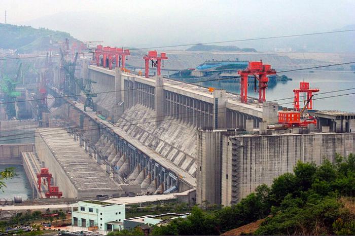

Bringing Down the Dams
There are clear cases for which the decision to remove a dam is virtually unquestioned except perhaps for its historical significance, said dam having outlived its usefulness. However, most proposals for dam removal are controversial because such decisions must evaluate benefits of retaining the dam against benefits of removing it. Certainly, these are complex decisions because of the conflict between ethical, economic, and legal aspects.
Enhancement of Populations of Anadromous Fishes
Enhancement of Populations of Anadromous Fishes
Dam removal has become increasingly popular, particularly as regards enhancement of populations of anadromous fishes--salmon and steelhead in the western U.S. and shad, herring and other species in the eastern U.S. Figure 13 illustrates the dams that have been removed in the lower 48 states (Figure 14 expands the eastern U.S.) from 1912 to 2023 on the basis of data tabulated by American Rivers [57]. These dams have been removed largely to improve the ecological conditions of river systems and to allow migratory fish to pass unimpeded for spawning in the upper reaches of rivers. Dam removal is commonly cited as a way of increasing stocks of imperiled fishes (Chesapeake Quarterly: Those Dammed Old Rivers [58]), allowing them to spawn in rivers that have been inaccessible to fish migration for as much as a century. Others argue that dam removal from coastal rivers is only part of the solution for fisheries improvements. Although numbers of anadromous fish may increase, the size of individual fish may not as long as fishing pressure remains the same (Oregon State University: Department of Fisheries and Wildlife [59]). This has been argued in the case of Elwha Dam removal in the Olympic National Park watershed (Crosscut: Elwha dams: Will bringing down NW dams really help salmon? [60]). In some cases, the benefits will accrue to native Americans who formerly depended on fishing for their nutrition and livelihood.
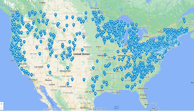
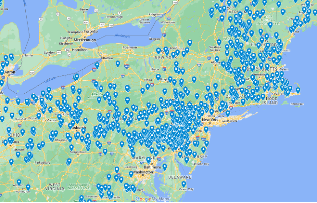
Esthetic Improvements
Esthetic Improvements
Arguments have also presented for esthetic improvements as the result of dam removal. An example of this approach is the argument for the removal of Hetch Hetchy (O'Shaughnessy) Dam on the Tuolomne River in the Sierra Nevada Mts. of California (Restore Hetch Hetchy [63]). This dam and its reservoir flooded a canyon much like Yosemite just to its south beginning in 1923, even though Hetch Hetchy was included in Yosemite National Park in 1890 by President W.H. Harrison. President Wilson, in 1913, signed the Raker Act that allowed San Francisco to dam the valley. Proponents of this dam removal argue for ecological improvements as well as access to once-spectacular scenery eliminated as the result of the water project. Hetch Hetchy provides some 20 percent of hydroelectric power generation to San Francisco as well as significant water supplies. Nonetheless, proponents of the dam removal argue that impacts on water or electrical power availability would be minor (Hetch Hetchy Today [64]).
Issues Accompanying Dam Removal
Issues Accompanying Dam Removal
One of the issues accompanying dam removal is the potential impact of the large volume of sediment that accumulated behind some dams over time. This so-called "legacy sediment" is commonly very fine-grained and contains stored nutrients and organic matter, among other possible pollutants. When dams are destroyed, efforts must be made to avoid a large flux of this sediment downstream as the newly released river cuts down to its natural base level. This requires careful engineering and significant funding. Merritts and Walter (2010) have suggested that most rivers and streams in eastern Pennsylvania and Maryland run through floodplains and levees of legacy sediment, not natural river valleys, created by the plethora of small dams built to impound water for hydropower in the past. And, even now, some large dams serve as a buffer against sediment transport that would create broad mudflats and high turbidity in coastal bays such as the Chesapeake Bay. Conowingo Dam in Maryland is one such structure that has reached its sediment capacity. During high flow events, sediments carrying nitrogen, phosphorus, and other pollutants enter the Chesapeake Bay. As of 2021, Maryland is working to implement a multi-million dollar strategy to reduce pollutants from entering the reservoir and reduce their flow downstream. For an example of the engineering and costs of removing a dam, check out the San Clemente Dam Removal & Carmel River Reroute Project [65] in central California.
Many dam removal projects are proposed, but await funding from federal sources—Congress must appropriate funds. Projects on the Snake River and the Klamath River in the west remain controversial, but at least in the case of the Klamath, the removal of four large dams has begun and it’s estimates that this will have lasting benefits on the river, community, and salmon populations. Figure 9 illustrates the consequences of waiting for funding of dam removal using the Olmstead Dam example.

In 1988, Congress authorized spending 775 million dollars for a 7-year project to build Olmsted Locks and Dam. But the cost has more than quadrupled to 3.1 billion dollars, and 25 years later, the project is barely half done.
| Year | Funds in millions |
|---|---|
| 1991 | 5 |
| 1993 | 60 |
| 1995 | 35 |
| 1997 | 70 |
| 1999 | 55 |
| 2001 | 60 |
| 2003 | 70 |
| 2005 | 75 |
| 2007 | 115 |
| 2009 | 115 + 5 in stimulus funds |
| 2011 | 140 |
| 2013 | 145 |
| 2014 | 163 |
The Future of Dams: Developing Nations
The Future of Dams: Developing Nations
As may be evident from a re-examination of Figure 1 above, the era of major dam building is winding down, at least in the U.S. This is primarily because the best sites for large dams are now already being used; and because the impacts are more widely understood and, as a result, proposed dam construction projects face major challenges from environmental groups. Construction of large dams (defined as those higher than four stories) in North America and Europe peaked in the 1970’s - and the average age of the worlds large dams is 35 years. Nonetheless, in parts of the world, mainly in developing nations in Africa, Asia, and South America, there is substantial untapped potential for hydroelectric power.
During the 1900s, in the so-called “golden age” of dam building, one large dam was commissioned somewhere on Earth every day (World Commission on Dams, 2000). On the one hand, dams are effective and powerful tools for water distribution and management, power generation, and flood control - and thus indirectly facilitate economic development, food production, and industrialization. Indeed, major dams are often viewed as symbols of modernization and progress - although a work of fiction, you may recall this quote from the movie “O Brother Where Art Thou”, as the protagonist, Ulysses Everett McGill, and his sidekicks are saved by the onset of a flood:
“Out with the old spiritual mumbo jumbo, the superstitions, and the backward ways. We're gonna see a brave new world where they run everybody a wire and hook us all up to a grid. Yes, sir, a veritable age of reason.”
Human Intervention in the Global Water Cycle
Human Intervention in the Global Water Cycle
On the other hand, as discussed above in Ponding the Waters: Impacts of Dams, the effects of large-scale alteration of river systems and the hydrologic cycle have become increasingly clear in the past few decades. The scale of human intervention in the global water cycle is also becoming apparent, including restriction of river flows such that they no longer reach the ocean in many years, associated two- or three-fold increases in the residence time of runoff, decreased sediment delivery to the oceans, and a long-term measurable effect on global sea level caused by the impoundment of thousands of cubic km of water (Vörösmarty et al., 2004). As a result, new large dam projects have been heavily scrutinized and faced political and environmental opposition. At the same time, the efficiency and economics of energy production, and the net offset of greenhouse gas emissions from increased hydropower generation have been increasingly questioned (World Commission on Dams, 2000). One way to minimize environmental impacts is to design “run of the river” systems, in which no reservoir is created and instead the natural flow of the river in its channel is harnessed to generate power. However, these systems have several drawbacks: they rely on natural flows, so the power generating capacity fluctuates dramatically as a function of seasonal rainfall patterns and climate change; and there are no added benefits of flood control or water supply.
Dams and Economic Development
Dams and Economic Development
Despite the controversy, in many developing nations, major dam projects remain important engines for economic development and hold substantial potential for renewable energy generation. As of 2020, hydroelectric power constituted as much as 17% of global electricity production (and 50% of estimated renewable energy production). Of this, ~23% is in China, ~12% in Brazil, ~10% in Canada, and ~7.5% in the United States; combined, these four nations generate over half of the world's hydropower!
Moreover, globally, estimates suggest that up to two-thirds of economically viable dam sites have yet to be exploited. Undeveloped sites are especially abundant in Latin and South America (79% of renewable water remains unused), Africa (96%), India and China (48% is unused in Asia) (UNEP, 2013). Rapidly growing energy demand in India, China, and the Amazon Basin have driven the construction of hundreds of large dams as of 2002 (Figures 10-11; Table 1). This development may be a harbinger of things to come on the African continent. Africa has the second-highest population (after Asia), and the fastest-growing (See Module 1.3); it also has the lowest per capita energy use (UNEP, 2013). Looking to the future as demand for energy, water, and food in developing nations continue to grow – both per capita and in total as populations swell - it seems inevitable that demand for large dams will persist well into the 21st century. Hydroelectric power provides 50% of electricity for 28 emerging and developing nations reaching over 800 million people.

| Region | Number of dams |
|---|---|
| China | 22000 |
| Asia | 9000 |
| North and Central America | 8000 |
| Western Europe | 4000 |
| Africa | 1000 |
| Eastern Europe | 1000 |
| South America | 800 |
| Austral-Asia | 500 |
| Country | Number of Dams | Purpose |
|---|---|---|
| India | 695-960 | Irrigation, multipurpose |
| China | 280 | Flood control, irrigation, power |
| Turkey | 209 | Water supply, hydropower |
| South Korea | 132 | Irrigation, hydropower, flood control |
| Japan | 90 | Flood control |
| Iran | 48 | Irrigation, multipurpose |
| Country | Number |
|---|---|
| China | 24,089 |
| United States | 10,158 |
| India | 4,540 |
| Japan | 3,135 |
| Canada | 1,440 |
| South Africa | 1,428 |
| Repbulic of Korea | 1,359 |
| Brazil | 1,280 |
| Mexico | 1,107 |
| Spain | 1,066 |
Data taken from CIG ICOLD [67]

Summative Assessment: Dam Debate
Instructions
We will build upon the online module content and written assignments for the Aswan High (Nile River), Three Gorges (Yangtze River), and Glen Canyon (Colorado River) Dams, and hold three in-class debates centered on the positive and negative impacts of each of three well known large dams. Students will break up to form small teams (2-3 members each) for each position (pro and con) for each of the three dams. At the end there should be 6 teams of 2-3 students, each taking the "pro" or "con" side on one of the dams. Each team will present their arguments in a format detailed below that allows for an exchange of views.
Thinking About Systems
Note that dammed rivers are complex systems, with many interlinked processes occurring up and down stream. When considering building a dam, all of these combined processes must be considered at once, making this a very tricky issue. Although you are trying to make a clear case for or against damming a river in the debate, resist the temptation to over-simplify the issue. Instead, force yourself to delve into the cascade of consequences building or not building a dam could have for a region - including agriculture, industry, energy, public health, etc.
Details
- Each team will have the opportunity to present their primary argument(s) [8 minutes].
- The arguments will be followed by a rebuttal [6 minutes].
- At the conclusion of each of the debates, the rest of the group will render their “opinions”.
- At the end of the class period, we will tally and discuss the outcomes.
We will consider a scenario in which the Three Gorges, Aswan High, and Glen Canyon Dams have yet to be built.
- Choose one of the three dams. Take a position for or against its construction, and develop the arguments to support your position. Draw upon the written assignments you completed as part of the online module.
- Your arguments and supporting material should reflect a clear understanding of the feedbacks between processes in the river system, and how dam construction would alter them. If your group is “against” dam construction, you’ll need to explain the negative aspects of disruption of the system. If your group is “for” dam construction, you’ll need to be ready to articulate and evaluate the effects of dams on inter-linked components of the river system, and construct arguments that weigh these against the benefits of dams.
- For whichever position you choose, articulate a plan to address the issues that you anticipate will arise if your course of action is adopted [i.e. be prepared to present a rebuttal of the opposing team’s arguments]. For example, if you argue against the Three Gorges Dam, how would you handle issues of flood control and potential loss of life and property? Would you attempt to offset the non-renewable energy generation that would replace hydroelectric power? If you argue for it, how would you address the range of environmental impacts?
- Prior to coming to class, prepare a one-page note sheet with factual information derived from the module and external reading (see References at the end of the Module) that you can use to support your argument. Be sure to include the source of each piece of information in case you are challenged!
- As an observer of other groups' debates, write a brief opinion (~1/2 page) with your “judgment” or “vote” on each of the debates you were not involved in. In each debate, which team convinced you of their position, and which arguments swayed you most? Do these apply to all large dam projects, or just those discussed in the debate?
Deliverables
1 page fact sheet (with references) supporting your argument
~1/2 page judgement or vote paper explaining which team made a stronger argument in each of the other two debates
Submitting Your Paper
Turn in your papers at the end of class.
Grading and Rubric
A scoring rubric will be provided by your instructor.
Module 6: Groundwater Hydrology
Module 6: Groundwater Hydrology
Overview
In this two-part module, we will focus on the occurrence and movement of groundwater. Key topics will include an overview of aquifer types and nomenclature, and the physical properties and processes that govern the storage, transport, rate of flow, and budgets of water in these systems. In addition, we will examine some examples of large-scale aquifer systems in the U.S., including those underlying the Valley & Ridge province and in the semi-arid American West. The module has two parts and is designed as a two-week course. The first section (Module 6.1) focuses on aquifers and their properties, with a series of case studies that outline the geometry and geology of highly-used regional aquifers. The second section (Module 6.2) focuses on the dynamics of aquifers, including the driving forces for water movement, flow rates, flow to pumping wells, and water budgets.
6.1 Aquifers and Properties
6.1 Aquifers and Properties
In the first part of this module, we will focus on the properties of aquifers: What characteristics of a rock or sediment make it a good aquifer? What are the different kinds of aquifers? Fundamentally, the ability to store and transmit water are the two key ingredients that make a subsurface geological formation useful as an aquifer. In Module 6.1, we will explore the detailed physical properties of rocks and sediments that ultimately affect the storage and movement of groundwater. We'll also illustrate with a series of well-known examples of large aquifers tapped for drinking, industrial, and agricultural uses.
Goals and Objectives
Goals and Objectives
Goals
- Explain the distribution and dynamics of water at the surface and in the subsurface of the Earth
- Interpret graphical representations of scientific data
Learning Objectives
In completing this lesson, you will:
- Identify the properties of artesian wells and describe the conditions under which they form
- Explain the difference between porosity and permeability
- List and describe the properties of aquifers that control the movement and storage of groundwater
- Explain the role of fractures in determining the transmission properties of aquifers
- Use Darcy's Law to explain the roles of aquifer properties and driving forces in governing the rate of groundwater flow
Aquifers Explained
Aquifers Explained
Aquifers come in many shapes, sizes, and “flavors”. For example, some aquifer systems span hundreds – or even thousands – of kilometers across several states or nations and may include multiple individual layers of rock or sediment that total thousands of meters in thickness. Other aquifers may be restricted to a few kilometers within a stream valley, and be only a few meters thick.
Nonetheless, there are some important common features of different kinds of aquifers. In this section of the module, we provide a basic overview of aquifers: What is an aquifer? What are the different types of aquifers, and what is their anatomy?
Overview and Nomenclature
Overview and Nomenclature
Aquifers are geologic formations in the subsurface that can store & transmit water (Figures 1 and 2). As we will see later in the section titles Basic Aquifer Properties, there are specific rock and soil properties that govern these two functions. Adequate storage requires that there be sufficient void space between particles, in fractures, or generated by compressing the aquifer under pressure, to provide usable quantities of water. Adequate transmission requires that the void spaces where water occurs be well enough connected that it can percolate or flow under either natural or pumping-driven conditions, at a rate that will support sustained use.


These definitions are intentionally vague because they depend on the scale of intended use. For example, an aquifer that provides water for a large city will need to sustain higher pumping rates at wells (on order of tens of thousands of gallons per minute) than one that provides for a single-family (a few to perhaps ten gallons per minute). For reference, Penn State University relies almost exclusively on groundwater pumping for its water supply at the University Park campus, with a total extraction of ~2.5 million gallons per day (about 1750 gallons per minute) distributed among several pumping well fields.
In contrast to an aquifer, an aquitard, often also termed a confining layer or aquiclude, is a geologic formation in the subsurface that does not transmit water effectively – and therefore acts as a barrier to groundwater flow. In general, aquifers are usually composed of sediments or sedimentary rocks with grain sizes larger than fine- to medium sand (>~125 µm diameter), or of fractured rock. Aquitards are typically composed of fine-grained sediments or sedimentary rocks or those in which the pore spaces have been filled by mineral cements (silts, siltstones, shales, clays, cemented sandstones, or unfractured limestones).
Aquifer Anatomy
Aquifer Anatomy
In the simplest sense, you might imagine an aquifer formation that may be covered by a veneer of soil, and which extends downward from a few feet below the surface for several tens or even hundreds of feet (Figure 3). At some depth below the land surface, the interstices between soil or sediment particles, or the fractures in the rock, will be water-filled or saturated. Shallower than that depth, these interstices, or pore spaces, will be filled with air, water vapor, and some liquid water bound to the surfaces of the rock (Figures 3-5). This zone is the unsaturated zone, also known as the “zone of soil moisture” or the vadose zone. The water table marks the top of the ground water system and is formally defined as the depth at which the pressure in the subsurface is equal to the atmospheric pressure. Immediately above the water table, there is a narrow zone of saturation termed the capillary fringe. In this zone, water is wicked upward in pore spaces due to capillary forces. This is analogous to capillary tube experiments you may have seen or performed in physics or chemistry classes in high school; it occurs due to interaction between the polar water molecule and the surfaces of the solids, and is directly related to the fact that water has a surface tension (as you may remember from Module 1!). In the capillary fringe, pores are saturated, but pressures are sub-atmospheric, meaning that the water is under suction as it is pulled or wicked upward. The nomenclature “fringe” reflects the fact that slight variations in grain size lead to variations in the height that water is drawn (again, think to the capillary tube experiment, and effects of different tube sizes) (Figure 5).
Any precipitation or surface water that infiltrates to the water table must percolate through the vadose zone in order to recharge the aquifer. As we will see later in this module infiltration and recharge typically constitute only a small fraction – rarely more than 10% - of precipitation, because most water that falls in events is returned to the atmosphere by transpiration or evaporation, becomes runoff (i.e., if the capacity for infiltration is exceeded by the rate of precipitation), or is bound by soils in the vadose zone.


Water (not ground water) held by molecular attraction surrounds surfaces of rock particles. All openings below the water table are full of ground water. The Unsaturated Zone is on the land surface and above the water table which contains the saturated zone, surface water, and ground water.
Types of Aquifers
Types of Aquifers
In more detail, there are three main classifications of aquifers, defined by their geometry and relationship to topography and the subsurface geology (Figures 6-9). The simple aquifer shown in Figure 6 is termed an unconfined aquifer because the aquifer formation extends essentially to the land surface. As a result, the aquifer is in pressure communication with the atmosphere. Unconfined aquifers are also known as water table aquifers because the water table marks the top of the groundwater system.
A second common type of aquifer is a confined aquifer, which is isolated from pressure communication with overlying or underlying geologic formations – and with the land surface and atmosphere – by one or more confining layers or confining units. Confined aquifers differ from unconfined aquifers in two fundamental and important ways. First, confined aquifers are typically under considerable pressure, which may be derived from recharge at a higher elevation or from the weight of the overlying rock and soil (known as the overburden). In some cases, the pressure is high enough that wells drilled into the aquifer are free-flowing. This condition requires that the water pressure in the aquifer is sufficient to drive water up the wellbore and above the land surface, and such wells are called artesian wells (Figure 7). Second, confined aquifers typically remain saturated over their entire thickness, even as water is removed by pumping wells. Water extracted from the aquifer comes only from the depressurization of the aquifer – a combination of depressurization and expansion of the water itself, and relaxation of the aquifer formation upon reduction in pressure (Figure 8).


The third main type of aquifer is a perched aquifer (Figure 6). Perched aquifers occur above discontinuous aquitards, which allow groundwater to “mound” above them. Thee aquifers are perched, in that they sit above the regional water table, and within the regional vadose zone (i.e. there is an unsaturated zone below the perched aquifer). The dimensions of perched aquifers are typically small (dictated by climate conditions and the size of aquitard layers), and the volume of water they contain is sensitive to climate conditions and therefore highly variable in time.

Aquifer Properties
Aquifer Properties
In the previous section, you’ve learned about the different types of aquifers, and the basic characteristics that define an aquifer – namely the ability to store and transmit water. But what, exactly, about a rock or sediment beneath the ground determines whether the rock can hold water, or whether water can percolate through it? In the following section, we will explore this question in more detail, to define the important individual properties of the rock.
Storage
Porosity (usually denoted by the symbol η, which is Greek letter 'eta') is the primary aquifer property that controls water storage, and is defined as the volume of void space (i.e., that can hold water in the zone of saturation) as a proportion of the total volume (Figure 10).


Porosity is expressed as either a fraction, or a percentage:
, or if reported as a percentage,
For aquifers composed of sedimentary rocks or sediments, porosity is usually in the range of ~10-35%. For unfractured crystalline rock, porosity is quite a bit lower - on order of a few percent - because there is little porosity between individual grains other than the vary narrow interfaces along their boundaries (Figure 10).
Several factors can affect porosity. In sedimentary rock and sediments, controls on porosity include sorting, cementation, overburden stress (related to burial depth), and grain shape. Poorly sorted sedimentary deposits, in which there is a wide distribution of grain sizes, typically have lower porosity than well-sorted ones (Figure 11). This is because the finer particles are able to fill in spaces between the larger grains. Cementation caused by precipitation of minerals (typically calcium carbonate or silica) at grain boundaries also reduces porosity (Figure 11). Angular grains generally allow more efficient packing of particles than rounded or spherical ones, also leading to slightly lower porosity. Finally, the more deeply sediments or sedimentary rock are buried, the larger the weight of the overburden; the higher stress leads to compaction, tighter packing of the grains, and lower overall porosity.
Secondary processes that act on the rock or sediment after its formation, primarily weathering by physical or chemical mechanisms, can also affect porosity. Physical weathering by wind or water movement can remove fine clay-sized particles from the sediment (a process termed winnowing), leading to increased porosity near the Earth’s surface. Chemical weathering of certain rock types can lead to clay and oxide formation; depending on the environment and initial composition of the aquifer grains, the clays and oxides may subsequently be removed (porosity increase), or they may grow at the boundaries of other particles and reduce the porosity.
In fractured rock (whether fractured crystalline or cemented sedimentary rock), porosity is typically ~2-5%. The pore space is almost entirely composed of the fractures or cracks themselves, which are typically a millimeter or less in aperture (Figure 12). Two primary factors control porosity – and the connectedness of porosity – in fractured rock. First, increased stress, related to the depth of burial and the weight of the overburden, exerts a clamping force that causes the closure of cracks or fractures (decreases fracture aperture). In some types of rock – most notably limestones – chemical weathering occurs via dissolution as water flows along and through fractures. This leads to increased fracture aperture. Significant enlargement of fractures can lead to the development of karst, typified by large open fractures, caves, and caverns, as well as sinkholes and hummocky topography that ensue as the underlying rock is gradually dissolved (Figure 13).
Interestingly, grain size does not affect porosity. For example, consider a box filled with spherical particles packed as tightly as possible. The proportion of empty space (porosity) would be the same whether the particles are marble-sized, pea-sized, or golf ball-sized; the porosity is controlled entirely by the geometry of the particles – not their dimensions. As we’ll see in the next section, however, grain size does strongly affect the ability of aquifers to transmit water because it directly controls the size of the pore spaces where the water percolates. For example, unconsolidated clays (grain sizes of a few to tens of microns) commonly have porosities of over 50-60%, but they transmit water only one-thousandth to one millionth as well as sands with porosities of 20-30% (grain sizes of a few hundred microns).
Specific Yield (denoted as Sy) is another important quantity for water storage in unconfined aquifers. Sy is defined as the proportion of water occupying void spaces that drains under gravity. Because some water is bound, or adsorbed, to the aquifer particles or fractures, the specific yield is always lower than the porosity (take a look at Figure 8 [74], inset at top left). The attraction between water molecules and the aquifer is due – you guessed it! – to the polar nature of water and surface tension. In sands and fractured rock, Sy is typically a large fraction (>90%) of the porosity, whereas in fine-grained sedimentary deposits Sy may be as low as a few percent because the surface area interacting with water molecules is higher, and pores are smaller, allowing the aquifer to retain more water. In unconfined aquifers, Sy controls the amount of water that can be extracted by pumping.
In confined aquifers, the compressibility of the aquifer is the dominant control on water storage and release. As described above (see Figure 8, right panel), when water is extracted from confined aquifers by pumping or flow to natural springs, the aquifer remains saturated, but the water pressure decreases. Upon depressurization, the aquifer itself can compress slightly. If water is recharged or injected, the opposite occurs: pressure increases and the aquifer expands very slightly. Essentially, by increasing water pressure, more water mass is being “crammed” into the pore space in the aquifer, and vice versa. Although exaggerated, one way to visualize this is to think of pores in the rock or aquifer as a juice box. By changing the pressure inside the box, it will expand or contract. In the same way that a soft juice box will deform more than a stiff one for a given change in pressure, a more compressible aquifer will yield more water than a stiffer aquifer, for the same depressurization. The storage of water in confined aquifers is termed the specific storage, and reported in units of Volume of water/Volume of aquifer per change in water level (so the units are 1/length; e.g., 1/m or 1/ft).


Sedimentary aquifers with intergranular porosity have groundwater storage between grains of sediment. Sedimentary aquifers with fracture porosity have groundwater storage in solution cavities.

Transmission
Transmission
The ability of an aquifer to transmit water – or of an aquitard to slow the flow of water – is the second essential ingredient controlling groundwater movement. It is also the most variable in natural materials; distances in astronomy are the only other quantity in nature that varies over a similar range! For example, the difference in groundwater flow rate for shale vs. gravel is a factor of 1,000,000,000,000 (yup…one trillion). That’s the difference between the size of an iPhone and the distance from the Earth to the Sun.
Groundwater transport properties are described by two related quantities. Hydraulic Conductivity, denoted by K, is a measure of the ability of a particular fluid (usually water) to flow through the rock or sediment. Permeability, denoted by a lower-case k, is often also termed “intrinsic permeability” and describes the ability of the geologic formation alone to transmit fluid. Although related, the key difference is that hydraulic conductivity combines properties of the geologic formation and the fluid, whereas permeability describes only the rock properties. As described in Sidebar 1, the basic concept of hydraulic conductivity emerged from a series of ingenious experiments conducted in the mid-1880s by Henri Darcy, a French Engineer. These experiments led to Darcy’s Law, which forms the foundation for much of modern hydrogeology and petroleum engineering.
To illustrate the difference between K and k, consider the sandstone in Figure 14 below. The sandstone itself has a permeability, which is controlled by the size of the grains and pore spaces through which water can percolate, and the connectedness and geometry of the pores (more on that in a moment!). That permeability is a characteristic of the sandstone, regardless of whatever fluid might be moving through it, the temperature, or anything else. But the flow rate of water through this sandstone will be different than for oil, or for air, or any other fluid. So the same sandstone also has a hydraulic conductivity specific to a given fluid of interest.

Viscosity and Density
Viscosity and Density
More specifically, it is the viscosity and density of the fluid that matter. More viscous fluids will flow more slowly through the same rock than less viscous ones. This is important for comparing different fluids (say, oil vs. water – whether you are thinking about an oil reservoir or contamination of groundwater by a gasoline spill). It is also important in considering the effects of temperature, because water viscosity decreases with increasing temperature: it’s less than half as viscous at 90° than at 32° F. So even for the same aquifer, the hydraulic conductivity goes up if it is warmer! This makes some sense – if the water is less viscous (i.e. “thinner”), it will flow more easily through the aquifer.
So…that’s how we define permeability and hydraulic conductivity. But what controls their magnitude? The main factors are grain size and shape, sorting, porosity (degree of compaction or fracture aperture), particle orientation or alignment that affects the tortuosity of the flow path, and cementation. Tortuosity is a measure of how far fluid must go to “circumnavigate” its way around particles: higher tortuosity indicates that water must go farther to get to its destination (a more tortuous path). For all of these mechanisms, the key underlying control on groundwater movement is the viscous resistance resulting from the interaction of the fluid with solid surfaces in the aquifer (grain edges or fracture walls).
Importance of Fractures
Importance of Fractures
Fractured aquifers are one important and widely used class of aquifer because they are commonly both highly permeable and rapidly recharged. For example, groundwater recharge to the limestone aquifer beneath Nittany Valley in the Spring Creek watershed is around 30-45% of the annual precipitation (in comparison to typical recharge of <10% of precipitation). Fractured aquifers are permeable despite their overall low porosity (usually <5%) because natural fractures usually form in consistent orientations and are well connected in networks over hundreds of meters to tens of kilometers or more (Figures 15-16). The preferred orientation of major fractures leads to anisotropy in permeability, in which the aquifer may be more permeable parallel to the dominant fracture directions than in other orientations.
The rapid flow rates and direct pathways for recharge from the land surface also lead to concerns specific to fractured aquifers. In the absence of confining layers or thick soils, rapid recharge along fractures that extend to or nearly to the land surface increase vulnerability of contamination by surface activity, including fertilization of fields, pesticide application, or spills. Direct connections between surface water bodies and groundwater through major fracture systems also increase the potential for water-borne pathogens to enter the groundwater system, especially during periods of high flow or if confining layers along stream beds are breached. Compounding this risk, if contamination does occur, flow along fracture networks can be very rapid and the direction and rates of contaminant transport difficult to predict - unless the fracture network in the subsurface is extraordinarily well known, which is rarely the case. Because of their potential for contamination, fractured aquifers are a subject of highly active research, including dedicated large-scale field programs (e.g., check out the U.S. Geological Survey’s Mirror Lake project [76]).

Regional Aquifer Systems: Examples
Regional Aquifer Systems: Examples
Ground water flow systems extend over a wide range of scales, from small perched aquifers that may supply water for a single-family, to regional rock formations that span thousands of km and cross several states (Figure 18). These regional systems supply water for irrigation and domestic uses in many areas, especially in semi-arid and arid parts of the American West and coastal population centers along the East coast (remember Module 1, figures 10-12?). These regional systems commonly consist of several layered sedimentary formations and may extend to several kilometers in depth. The U.S. Geological Survey has compiled detailed studies of regional aquifer systems across the U.S., with useful information about climate, recharge, subsurface geology, use, and problems related to water quality or quantity (a list and links for each of the principal regional aquifers in the U.S can be found at USGS Groundwater Information [78]. A detailed atlas with information about the major aquifer systems in particular regions of the U.S. can be viewed at USGS Ground Water Atlas of the United States [79]. In this module, we will focus on a few example regional aquifer systems of particular relevance to the Northeastern and mid-Atlantic U.S. and the Central Valley of CA.
Valley and Ridge Aquifer System
Valley and Ridge Aquifer System
The Valley and Ridge aquifer system extends SW-NE across Central PA, West VA, and VA (Figure 19, purple area), and is the main water supply for much of this region. It is composed of layered Paleozoic sedimentary strata (shales, sandstones, and limestones) that were folded and deformed by a series tectonic collisions over 200 million years ago. The modern valleys in the Valley and Ridge province have formed where limestone, which is most susceptible to erosion, was exposed in the core of anticlines, or upfolds (Figure 20). The more resistant sandstones and shales form the regional ridges, like Mt. Nittany and Bald Eagle Ridge.
The principal aquifer unit in this system is the fractured limestone that underlies the valleys. As noted above, because it is fractured, it recharges rapidly, has a high fracture permeability, and wells drilled along the fractures are highly productive (c.f. Figure 17). Recharge is focused on the flanks of the ridges, where runoff flows over the less permeable shale and sandstone units and enters the groundwater through fractures or sinkholes above the limestone at the valley edges. Groundwater flow is generally toward the center of the valleys, and springs commonly feed the surface water systems. The water is characterized by a high hardness (Mg and Ca content; we’ll cover this in more detail in Module 7), derived from limestone dissolution. Dissolution of the limestone has formed extensive karst features (caves, caverns, sinkholes) throughout the region.


The Paleozoic rocks of the Appalachian Plateaus and the Valley and Ridge Provinces range from nearly flat-lying to intensely folded They are commonly separated from crystalline rocks of the Blue Ridge and the Piedmont Provinces by faults. The sediments of the Coastal Plain Province overlie older rocks and dip gently toward the ocean.
Atlantic Coastal Plain Aquifer System
Atlantic Coastal Plain Aquifer System
The Atlantic Coastal Plain aquifer system extends North-South along much of the Eastern portions of New Jersey, Delaware, Pennsylvania, Virginia, and North Carolina (Figure 19). It consists of a sequence of layered sedimentary aquifers (sands and gravels) separated by series of aquitards, all deposited starting around 100 million years ago and continuing today. The layers slope, or dip, to the East and extend offshore for tens of km beneath the continental shelf (Figure 21).

Recharge occurs by both natural and managed infiltration on land across much of the coastal plain; groundwater flow in the subsurface is mainly to the East along the sediment layers. One interesting consequence of this flow pattern is that there may be a sizable freshwater resource offshore that could be accessed by drilling in relatively shallow water on the continental shelf. During the last ice age, when conditions were substantially wetter than today and a nearly mile-thick ice sheet covered the northern extent of the aquifer system, recharge was probably even larger - and thus may have forced fresh water several tens of km offshore, where that “fossil” water may remain today!
The Atlantic Coastal Plain system is an important water source for domestic/municipal supply and industry in population centers throughout coastal North Carolina, Maryland, Virginia, Delaware, and New Jersey. However, concentrated, localized pumping has led to a reversal of flow direction (toward the wells instead of Eastward) in some of the aquifer units throughout the region. In addition to overarching concerns about the sustainability of withdrawals that exceed recharge rates, the flow reversal has led to local salt-water intrusion, whereby saline ocean water infiltrates the aquifer and in some cases renders it non-potable.
Central Valley/San Joaquin Valley Aquifer System
Central Valley/San Joaquin Valley Aquifer System
The Central Valley Aquifer system of Central CA lies in a large structural basin running approximately North-South, between the Coast Ranges to the West and the Sierra Nevada mountains to the East (Figure 22). The deep elongate basin is infilled with marine and continental sediments, primarily composed of interlayered sands and clays. The basin itself is formed by tectonic processes caused by East-West extension (these are the same forces that are causing continued uplift of the major mountain chains throughout the Basin and Range province of the Southwestern US, and which are one major control on orographic precipitation patterns in that region).
The continental deposits (Figure 22, orange) comprise the main aquifer units and range from one-half to over two miles in thickness. As is the case in the Valley and Ridge, the recharge is primarily focused around the valley perimeter as runoff over the flanks of surrounding high topography infiltrates and enters the groundwater system. Groundwater flow is primarily inward, toward valley center, with a component of flow down-valley to the North, parallel to surface water flow in the San Joaquin River.


The thick sedimentary sequence has formed a vast expanse of flat topography on the natural floodplain of the San Joaquin River. This, in combination with a mild climate that allows a year-round growing season, has made the Central Valley one of the most productive and largest agricultural centers in the world. The Central Valley aquifer system is highly utilized, primarily to augment limited allocations of surface water for irrigation. Since the mid-1920s, groundwater withdrawals have generally outpaced natural recharge to the aquifer, leading to dropping water levels, irreversible aquifer compaction, and land subsidence (as will be discussed in more detail next week, in Module 6.2). Until recently, groundwater withdrawals were neither heavily monitored nor regulated. However, in the face of an ongoing multi-year drought, a 2014 bill was signed into law that restricts pumping and implements groundwater sustainability plans (See What to Know about California's New Groundwater Law [81]; see also New California Groundwater Pumping Rules Signed Into Law [82]). Shallow aquifer units in the valley are also plagued by a wide range of water quality concerns associated with irrigation and return flow of irrigation water to the aquifer via infiltration; these include leaching of selenium, boron, and other constituents from soils; salinization; and high concentrations of pesticides and fertilizers. We’ll discuss all of these issues in more detail in upcoming modules about water quality and the effects of climate change.
Darcy’s Experiments and Darcy’s Law
Darcy’s Experiments and Darcy’s Law
In 1855, Henri Darcy, a French hydraulic engineer (Figure 24), oversaw a series of experiments aimed to understand the rates of water flow through sand layers, and their relationship to pressure loss along the flow paths. Darcy’s experiments consisted of a vertical steel column, with a water inlet at one end and an outlet at the other. The water pressure was controlled at the inlet and outlet ends of the column using reservoirs with constant water levels (Figure 25) (denoted h1 and h2). The experiments included a series of tests with different packings of river sand, and a suite of tests using the same sand pack and column, but for which the inlet and outlet pressures were varied. For part of our in-class activity this week, we will perform our own set of “Darcy Tube” experiments, and also work with the original dataset generated by Darcy in his experiments.


Darcy’s findings laid the foundation for the modern science of hydrogeology by quantifying the relationships between volumetric groundwater flow rate, driving forces, and aquifer properties. Specifically, Darcy’s experiments revealed proportionalities between the flux of water, Q, through the laboratory “aquifer” and different characteristics of the experimental system (refer to Figure 25 above):
Q was directly proportional to the difference in water levels from inlet to outlet, :
- Q was directly proportional to the cross sectional area of the tube:
- Q was inversely proportional to the length of the column:
Combining these proportionalities leads to Darcy’s Law, the empirical law that describes groundwater flow:where K is a constant of proportionality that defines the water flux for a given hydraulic gradient . The above equation can also be recast in terms of the water volume flux per unit area, Q/A (also called "Darcy flux" or "Darcy velocity" with units of length per time):
6.2 Aquifer Processes and Dynamics
6.2 Aquifer Processes and Dynamics
In the first half of the module, we’ve explored the properties of aquifers. But, of course, that is only half of the story! In order for groundwater to flow, there must be a driving force. The same is true for surface water like streams or rivers: in that case, the driving force is gravity. In the case of groundwater, the driving force is a bit more complicated because it includes the combined effects of gravity and pressure.
As we will see, these driving forces are partly determined by the natural system but can be perturbed by pumping or injection in wells. When we pump water from wells, we alter the natural driving forces to move water toward the well. One important issue in aquifers is accounting for the flows in to and out of the aquifer in a groundwater budget. In extreme cases, the amount of water extracted at wells may exceed the amount introduced to the aquifer through recharge. As we’ll discuss, this tenuous condition is known as an overdraft.
Goals and Objectives
Goals and Objectives
Goals
- Describe the two-way relationship between water resources and human society
- Explain the distribution and dynamics of water at the surface and in the subsurface of the Earth
- Thoughtfully evaluate information and policy statements regarding the current and future predicted state of water resources
- Interpret graphical representations of scientific data
Learning Objectives
In completing this lesson, you will:
- Apply the concept of hydraulic head to draw flowlines on maps and cross-sections
- Interpret the current and historical balance between groundwater recharge and water extraction from well hydrographs
- Propose a course of action to address overdraft in an aquifer
Driving Forces for Groundwater Flow
Driving Forces for Groundwater Flow
The driving forces that control groundwater flow are a bit more complicated than those controlling flow in rivers and streams. As you learned in Module 3, surface water flows downhill due to gravity, and the flow direction is defined by the topography. Water flows downhill because gravity is a form of potential energy – and the water, or anything that falls or rolls downward – flows in response to differences in potential energy (from high to low).
In contrast to surface water, groundwater is separated from the atmosphere, and as a result, it can be under considerable pressure. Therefore, the potential energy that drives groundwater movement includes both pressure and gravity. In this section, you will learn about these driving forces, how we define them, and how they translate to the direction and rate of groundwater movement in the subsurface.
Potential Energy and Hydraulic Head
Potential Energy and Hydraulic Head
The flow of both surface water and groundwater is driven by differences in potential energy. In the case of surface water, flow occurs in response to differences in gravitational potential energy caused by elevation differences. In other words, water flows downhill, from high potential energy to low potential energy. In groundwater systems, things are a bit more interesting. Unlike surface water, which is in contact with the atmosphere and therefore rarely under pressure, water in groundwater systems is isolated from the land surface. This means that groundwater can also have potential energy associated with pressure. In extreme cases, water in confined aquifers may be under sufficient pressure to drive flow upward, against gravity. Artesian wells are one manifestation of this.
Fundamentally, groundwater and surface water are similar in that flow is in the “downhill” direction. But what does “downhill” mean in a groundwater system? To define the flow direction, we need to account for the two types of potential energy. Unfortunately, the potential energy of the water cannot be measured directly. However, we can measure a proxy for the potential energy by measuring the hydraulic head, or level to which water rises in a well (Figures 26 and 27). The hydraulic head combines two components: (1) potential energy contained by the water by virtue of its elevation above a reference datum, typically mean sea level; and (2) additional energy contributed by pressure. In a well, the value of hydraulic head represents the potential energy of the water at a particular point in three dimensions – at the depth where the well is open to the aquifer (Figures 26-27). This is analogous to a temperature reading taken at the tip of a thermometer, which provides a proxy for heat energy. Hydraulic head can be written as:
h = z + Ψ,
where z is the elevation energy, and Ψ is the pressure energy.


Click to expand to provide more information
Hydraulic Head and the Direction of Groundwater Flow
Hydraulic Head and the Direction of Groundwater Flow
In order to define groundwater flow directions and rates through aquifers, individual measurements of hydraulic head are combined to generate contour maps of water level – or potential energy (Figure 29). These maps define the potentiometric surface, which is much like a topographic contour map but defines the distribution of potential energy in the groundwater system. Each contour, or equipotential, represents a line of equal hydraulic head.
Video: Slag Heap Experiment (3:46 minutes)
To first approximation, groundwater flows down-gradient (from high to low hydraulic head). As is the case with surface water, or a ball rolling down a hill, the water flows in the direction of the steepest gradient, meaning that it flows perpendicular to equipotentials. There are exceptions to this – for example, if the hydraulic conductivity of the aquifer is much higher in one direction than another, or dominated by fractures with particular orientations, then these can redirect groundwater flow askew to the maximum gradient.
The potentiometric map also provides clues about the rate of groundwater flow. If you think back to Darcy material and our in-class activity from last week, you will recall that groundwater flow rate depends on the head gradient (i.e. the hydraulic gradient) and hydraulic conductivity. In a simple one-dimensional Darcy tube experiment, the head gradient is just the difference (h1-h2)/L. In two dimensions, the head gradient is defined by the slope of the potentiometric surface – just as the slope of the land surface is defined on a topographic map. The path that water takes in the aquifer, defined as a continuous line tracing the maximum gradient on a map of the potentiometric surface, is known as a flowline.
Well Hydrographs
Well Hydrographs
Just as river hydrographs are used to record and visualize variations in flow with time (as discussed in Module 4), a well hydrograph is a time series of hydraulic head recorded in a well. This provides information about the fluctuation of hydraulic head (equivalent to the water table in an unconfined aquifer), which reflects the combined effects of temporal variations in climate, recharge, and pumping (Figures 30-31). The U.S. Geological Survey maintains a database of active monitoring wells [83] in major aquifer systems across the United States. Hydrographs provide information about seasonal patterns that may be associated with pronounced wet and dry seasons typical of some regions (for example, Central CA), as well as long-term trends driven by climate change, decadal-scale climate patterns like el nino, prolonged groundwater extraction, or human-induced modifications to natural recharge. We’ll cover examples of the latter two processes in the next section of the module (Module 6.2: Water budgets).
USGS [85]
Video: Slag Heap Experiment (3:46)
Now that we've thought about how and why groundwater is moving through this system, we want to use the groundwater model to make some predictions about how a contaminant would move through the groundwater system. Let's imagine our model represents a geologic cross-section under the East Helena smelter site, and we want to think about how contamination from the slag heap would move through the groundwater system.
So, this slag heap was rained on. Arsenic and selenium from the slag would leach into the groundwater system. How do we think that contamination will move through this system and why? Take a minute to think about how and why contamination will move through this groundwater system.
Okay, so now we're going to add some dye at the location of the slag heap and see where that contamination moves in our model of a groundwater system.
Effects of Pumping Wells
Effects of Pumping Wells
Groundwater is accessed by either pumping from wells drilled into the aquifer (Figure 33), or by developing natural springs where the potentiometric surface intersects the land surface (Big Spring in Bellefonte, PA is one example of a relatively large spring that is used for municipal supply). Although springs are relatively inexpensive to develop, they are not always present, nor are the flow rates always sufficient to support demand. As a result, most groundwater extraction occurs by pumping wells, or in many cases “fields” of wells concentrated in a small area.

Cones of Depression: Pumping at a well, or at a wellfield, pulls water toward the well from all directions – in other words, it induces radial flow (around the radius of the well). In doing so, pumping causes a reduction in hydraulic head, known as drawdown. This drawdown generates a cone- or funnel-shaped depression called a cone of depression (Figure 35). The reduction in hydraulic head drives groundwater flow to the well (in the down-gradient direction), as shown in the example from Long Island in Figure 36.


Both the width and the depth of the cone of depression scale with the rate of pumping, the aquifer permeability, and storativity, and the duration of pumping. In general, larger cones of depression result from larger pumping rates, higher permeability or lower storativity, and longer elapsed time. If cones of depression from two separate pumping wells grow large enough to overlap, it is known as well interference. When well interference occurs, the respective drawdowns are added together. The result is that drawdown is accelerated when multiple cones of depression interact. This is generally not desirable, and is one important consideration in the design, permitting, and operation of wells.
Not only does the cone of depression draw water to the well, but if the pumping rate is large enough or pumping is sustained for a long time, it can reverse the natural hydraulic gradient hundreds of meters to several tens of km away from the well(s). In some cases, this may result in interception of groundwater that would normally feed a stream or river as baseflow, and even in the interception of streamflow itself by inducing infiltration in the stream bed or banks (Figure 35B). In other cases, large cones of depression (up to a few miles wide!) associated with industrial or municipal well fields may reverse regional topographically-driven hydraulic gradients and lead to problems like saltwater intrusion (Figure 35B).
Groundwater Budgets
Groundwater Budgets
Now that you are an expert on how groundwater flows, we will apply that knowledge to the important problem of groundwater budgets. As groundwater flows through and exits an aquifer, for example at springs or at extraction wells, those losses of water may be balanced by recharge that percolates from the land surface. As you’ll investigate in the following section, and through a case study of the famous Ogallala aquifer in the American Midwest, understanding the budget of inflows and outflows to an aquifer is critical to evaluating the sustainability of groundwater use.
Fluxes (Inflows and Outflows) in Groundwater Systems
Fluxes (Inflows and Outflows) in Groundwater Systems
Fluxes (inflows and outflows) in Groundwater Systems: In order to define the water balance or water budget of an aquifer system, the individual processes that bring water into or out of the system must be quantified (Figure 37 on the next page).
Common inflows of water to a groundwater system include:
- Infiltration through the vadose zone that is not intercepted by evaporation, transpiration, or bound in the unsaturated zone, and thus becomes recharge. Infiltration may be distributed over large areas, or may be focused beneath surface water bodies or at geological features (e.g., sinkholes). Recharge may occur naturally or can be induced or enhanced by excavation and removal of low-permeability soils, and the construction of recharge pits, typically lined or filled with permeable sands (Figure 38 on the next page).
- Injection at wells, either for disposal of treated wastewater or as part of managed aquifer storage and recovery (ASR) programs. The latter is growing in popularity as one way to “bank” excess water in times of surplus, for example, wet seasons or wet years, and then tap the stored water when needed. Although energy-intensive because it requires pumping, ASR is not affected by evaporative losses whereas reservoirs are.
- Groundwater flow from areas outside of the region of interest – areas that are either up-gradient or above or below (i.e. flow across a confining layer).
Outflows from groundwater systems typically include:
- Evaporation or transpiration; this typically occurs in areas where the water table is shallow. Although direct evaporation of water from the water table is possible (in detail, this would occur by evaporation from the capillary fringe, and subsequent “wicking” of water upward from the water table), the upward flux (loss) of water from unconfined aquifers to the atmosphere is dominated by a family of plants known as phreatophytes, characterized by deep roots that extend to and below the water table.
- Water withdrawal by pumping from wells. As discussed in the previous section, pumping at wells induces radial flow toward the well. As the cone of depression grows, the well accesses water over a larger region of the aquifer. In some cases, as the cone of depression grows it may intercept water that would otherwise exit the aquifer via natural seeps or springs (e.g., Figure 37 on the next page), thus “redirecting” a flux that would have been an outflow somewhere else.
- Natural groundwater flow or discharge at springs or seeps, or to surface water bodies.
Surface Water-Groundwater Interaction
Surface Water-Groundwater Interaction
One specific class of inflow or outflow from groundwater systems results from surface water–groundwater interaction, water flows from aquifers into surface water bodies at seeps or springs, or infiltrates from rivers or lakes into aquifers (Figure 39; also note the dual-sided arrow between the aquifer and stream in Figure 37 indicating that the flux may be either to or from groundwater to surface water). If there is a net groundwater flux to surface water, the surface water body is said to be gaining (for example, a gaining stream is one that is fed by groundwater). As you may recall from Module 4, the component of streamflow derived from groundwater influx is termed baseflow. Alternatively, if the water table lies below the surface water body, the potential energy (hydraulic head) in the surface water body will be higher than in the groundwater system and water will percolate downward to the aquifer. In this configuration, the surface water body is said to be losing (i.e. a losing stream), because the stream or river discharge decreases downstream. While the land surface and stream channel generally remain at the same elevation, the water table commonly fluctuates over time (see Figures 32-33). As a result, it is common for streams to alternate between gaining to losing due to major recharge events, seasonality in precipitation and recharge, and variations in pumping rates.
Although water rights and policies are sometimes constructed with the implicit assumption that surface water and groundwater systems act independently, this is clearly not the case. A number of interesting situations arise from their interaction. As noted above in the Effects of Pumping Wells section, pumping at wells can reverse groundwater flow, and change a gaining stream to a losing one. In such a scenario, it isn’t always clear whether surface water rights are violated by groundwater pumping – even though groundwater extraction directly causes a reduction in surface water discharge, the water is withdrawn from the groundwater system, not the river. In large aquifer systems, the intercepted baseflow may impact users far downstream, across county and state borders. In other cases, also as noted earlier in this module, substantial or rapid influxes of surface water to groundwater systems, for example through fractures or sinkholes, can lead to groundwater contamination. If a direct connection between surface water and groundwater is demonstrated by the presence of microorganisms or increased water turbidity (cloudiness indicating suspended particles) in well water, additional treatment of groundwater is required before it is considered suitable for domestic or municipal use.


Water Budgets
Water Budgets
The balance of water inflows and outflows, or water budget, for a groundwater system, is described by a simple equation:
where I is the total of the inflows to the system, O the total outflows and ΔS is the change in storage. The water balance equation is no different than a bank statement: the difference between deposits (inflows) and withdrawals (outflows) is equal to the change in the account balance (storage). In the case of groundwater systems, changes in storage are manifested as changes in the potentiometric surface, either due to drop in the water table (in unconfined aquifers) or reduction in elastic storage as aquifer is depressurized (in confined aquifers).
In a steady state, or equilibrium condition, inflows and outflows are perfectly balanced (i.e. I = O in the budget equation above), and ΔS is zero. In other words, the potentiometric surface is steady. Often, groundwater systems are considered to be at steady state if inflows and outflows balance over a yearly or decadal timescale. This is because, in many aquifers, both recharge and extraction may be strongly seasonal. For example, recharge in many aquifers in the western US is mostly restricted to the winter months when precipitation is highest, and withdrawal rates are highest in the summer and early fall dry season. As a result, the potentiometric surface may fluctuate over the course of the year but is more-or-less constant over the long-term.
A variety of processes can lead to non-steady state conditions. Most notably in aquifers that are used heavily for irrigation, industry, or municipal supply, pumping may significantly exceed recharge, leading to net decreases in storage. In other cases, reduced recharge – for example due to urbanization and construction of impervious surfaces that do not allow infiltration, removal of leach fields upon installation of sewers (Figure 30), or long-term climate trends that drive changes in the amount or timing of precipitation – also results in negative changes in storage. Reductions in groundwater extraction, or periods of increased precipitation, will have the opposite effect and lead to increases in storage.

Overdraft
Overdraft
Groundwater overdraft is a specific condition in which extraction greatly exceeds the influxes of water (mainly recharge). This produces an unsustainable condition characterized by sustained declining water levels. Much like overdraft of a bank account, groundwater overdraft is not a desirable state of affairs. Not only is it unsustainable in terms of management of the groundwater resource, but it also leads to long-lasting damages (a lot like what happens to your credit rating if your bank account is overdrafted!).
Depressurization of the aquifer, if large enough, may cause irreversible collapse and compaction. This reduces both storage (porosity) .and hydraulic conductivity. It can also lead to land subsidence, especially in cases where the magnitude of overdraft is large and the aquifer units are thick and highly compressible, as is common for unconsolidated or uncemented sedimentary aquifers. One well-known example of groundwater overdraft is the Central Valley of California (Figure 41). Another is the Ogallala aquifer, a major groundwater system spanning across eight states in the American Midwest (Figure 43; see The High Plains Aquifer section). Substantial overdraft and subsidence also occur in widespread areas of the southeastern U.S., the Gulf Coast, and parts of Arizona and Las Vegas (Figure 44).


The High Plains Aquifer
The High Plains Aquifer
The High Plains Aquifer system consists of Tertiary sedimentary rock, dominantly sandstone and gravel (Figure 45), eroded from the ancient Rocky Mountains and deposited in the Tertiary period (from about 31 to 5 million years ago). The Ogallala Formation is the primary aquifer unit in the system. The aquifer underlies almost 175,000 mi2 and spans eight states, with most of its area in Nebraska, Texas, and Kansas. This region is among the largest and most productive croplands in the U.S. and is the source of almost 20% of our corn, wheat, and cotton production, as well as a significant portion of our soybeans, sorghum, and alfalfa. It is also host to almost 20% of the cattle raised in the US. Because the climate is semi-arid, with mean annual precipitation ranging from 12 inches in the West to 33 inches in the East, growing economically viable crops requires substantial irrigation. If you have ever flown over the Midwest on a clear day you may have seen circular “patches” of irrigated land - the hallmark of center-pivot irrigation systems (Figure 46).
Although farming has been a major part of the economy in the region since the late 1800s, in the 1960’s new technology in electrical pumps allowed access to deeper groundwater and ushered in an era of rapidly expanding irrigated acreage (Figure 47). Accompanying this expansion, aquifer-wide groundwater withdrawals increased from a few million acre-feet (M-AF) per year to almost 20 M-AF. Water level declines began in the 1950s, with the onset of intensive groundwater extraction for irrigation-based agriculture. The total overdraft of the aquifer is almost 287 million acre-feet, from pre-development (ca. 1950) to 2019 – this is over 17 times the annual flow of the Colorado River.


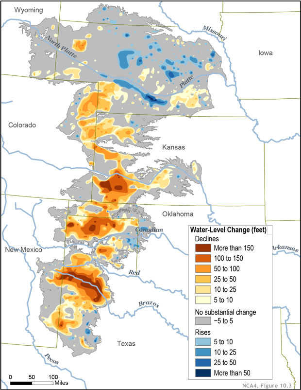
As a consequence of sustained overdraft for several decades (see Figure 44 above), water levels in the aquifer have dropped substantially, by more than 100 feet in many areas (Figure 48). Over half of this decline has occurred since 2000. Water level declines are not evenly distributed, however. The highest rates of decline are focused in the southern reaches of the aquifer system, where recharge rates are low and irrigation demand is highest. In the northern portions of the aquifer system, water level declines are considerably smaller – and in some cases, the water table has actually risen – primarily due to locally higher recharge focused along the Platte River (Figure 48).
Capstone Project Introduction
Capstone Project Introduction
Looking Forward: Capstone Project Expectations
For your Capstone Project in this class, you will be developing a water plan for a water-critical city of your choosing. The assignment includes a 10-slide presentation (no more) and written report (including at least 5 significant references). If you would like to read a more detailed description of the Capstone Project, you can look ahead to the Capstone Project [95] at the end of Unit 3. For right now, the critical thing is that you choose the city for which you would like to develop a water plan and submit your selection in Canvas using the discussion thread in the Unit 2 Reflection module [week 9] module. A list of cities to choose from is provided below. Requests for other cities will be considered if you can provide justification for your selection.
Instructions
- Pick a city from the list below or propose one: (note: if you are proposing a new city, you must check with us first by sending an email via Canvas including the name of the city and the water concerns.
- Los Angeles, CA
- San Diego, CA
- San Francisco, CA
- Las Vegas, NV
- Tucson, AZ
- Denver, CO
- Flint, MI
- Miami, FL
- Delhi, India
- Dubai, UAE
- Mexico City, Mexico
- Sao Paolo, Brazil
- Khartoum, Sudan
- Nairobi, Kenya
- Beijing, China
- Cairo, Egypt
- London, England
- Bangalore, India
- Tokyo, Japan
- Tehran, Iran
- Submit your selection via Canvas using the discussion thread in the Week 9 folder.
Unit 3: Social Science of Water
Unit 3: Social Science of Water
Overview
Congratulations! You have completed the first two units of the "Water: Science and Society" course. Having done so, you are prepared to tackle some serious issues with respect to fresh-water resources, both in the U.S. and globally. Unit 3 comprises four modules (7-10) that are spread over five weeks of the semester. These modules present an overview of the water supply challenges that face society now and in the future, and prompt you to explore possible solutions to those challenges.
Module 7 ("What's In Your Water?") delves into the role of water as a "universal solvent" and the problems that its ability to dissolve and transport nearly any potential chemical pollutant present for drinking water quality, water quality in natural environments, and agricultural activities. The module offers several short "case studies" whereby human activities alter the chemistry of surface- and/or groundwater, creating toxic conditions for humans and wildlife (e.g., so-called "dead zones" in coastal regions), and asks you to consider possible solutions to these and other water quality problems through regulation or process changes.
Module 8 ("Cities in Peril: Dealing with Water Scarcity, Part 1: History and Current Approaches, and Part 2: Future Growth and Climate Change") covers two weeks of the course and focuses on the problems of major population centers with respect to acquiring clean drinking water. Understandably, the problem is more extreme for large cities located in arid regions (e.g., Los Angeles, CA or Las Vegas, NV), but is not governed simply by water availability. Infrastructure construction and maintenance is another related issue. There is also strong pressure on fresh water availability from prolonged drought, which could result from global climate change. The second part of Module 8 introduces climate change as a factor, what we understand now, and how well we can predict future changes.
In Module 9 ("Water and Politics: International Issues") we entertain the human penchant for laying claim to water resources, and the need to fairly "share" resources in cases where rivers (or groundwater basins) cross international borders (or in some cases, rivers that are the basis for international borders), while also protecting water quality. Are old treaties adequate as governments change and populations grow? Will we experience further "water wars?" The Nile River in northeast Africa and the Colorado River in western North America are good examples.
Module 10 ("Solving the Water Crisis? Potential Solutions to Problems with Water Scarcity and Quality") is the culmination of the course, bringing together diplomacy, economics, and technology to explore potential solutions for fresh water shortages. Some of these solutions, although elegant and high-tech, will not be feasible where funding and energy are in short supply. You will evaluate these possibilities and recommend a path forward.
Modules
- Module 7: What Is In Your Water? [96]
- Module 8: Cities in Peril: Dealing with Water Scarcity [97]
- Module 9: Water and Politics: Global Issues [98]
- Module 10: Solving the Water Crisis? [99]
Unit Goals
Upon completion of Unit 3 students will be able to:
- Describe the two-way relationship between water resources and human society.
- Explain the distribution and dynamics of water at the surface and in the subsurface of the Earth.
- Synthesize data and information from multiple reliable sources.
- Interpret graphical representations of scientific data.
- Identify strategies and best practices to decrease water stress and increase water quality
- Thoughtfully evaluate information and policy statements regarding water resources
- Communicate scientific information in terms that can be understood by the general public
- Predict how the availabilty of and demand for water resources is expected to change over the next 50 years
Module 7: What is in Your Water?
Module 7: What is in Your Water?
Overview
Water is the "Universal Solvent." Virtually every element on the periodic table and many organic substances (molecules) are soluble (can be dissolved) to some degree in water. Many substances occur "naturally" in water—that is they are dissolved into water as it flows over rock surfaces or through aquifers in the subsurface or as it mixes with other waters. Some substances are "pollutants," having been added as the result of certain human activities, intentionally or unintentionally, including wastewater (untreated) disposal, drainage of acidic waters from abandoned mines, drainage from agricultural operations (e.g. manure, herbicides, pesticides), etc. "Water quality" implies an assessment of the degree of contamination of a water source by direct measurement of its dissolved components. Not all dissolved components in water are harmful to human health, but this depends, in part, on their concentration. In this module, we will explore some of the science and issues with respect to drinking water quality, a bit about the chemistry of natural waters, and the regulations that help ensure a satisfactory drinking water supply for the U.S. populace. In addition, we will outline some water quality issues that affect other parts of the globe.
Goals and Objectives
Goals and Objectives
Goals
- Describe the two-way relationship between water resources and human society
- Explain the distribution and dynamics of water at the surface and in the subsurface of the Earth
- Synthesize data and information from multiple reliable sources
- Interpret graphical representations of scientific data
- Identify strategies and best practices to decrease water stress and increase water quality
- Thoughtfully evaluate information and policy statements regarding water resources
- Communicate scientific information in terms that can be understood by the general public
Learning Objectives
In completing this module, you will:
- Calculate the concentration of contaminant in a reservoir
- Apply government drinking water regulatory standards to identify contaminant levels that might be harmful to human health
- Analyze concentration vs. time data for various dissolved components of river water and ground water
- Infer the processes responsible for seasonal trends in compounds of natural and human origin
- Propose and evaluate methods for mitigating human impacts on water quality
- Evaluate the tradeoff between agricultural productivity and water quality as a result of fertilizer usage and runoff
Units of Water Chemistry
Units of Water Chemistry
Elements and molecules have solubilities (the amount that can be dissolved in water before the water is saturated with that element and no more can be held in solution) that depend on their individual properties and styles of bonding to other elements. For example, common table salt (NaCl), when added to water, will dissociate into individual charged ions of Na+ and Cl-. These are held apart from one another "in solution" because they are surrounded and isolated by polar water molecules (Unique Properties of Water section).
Distilled water or "pure" water typically has near-zero concentrations of other components. If concentrations of dissolved elements or compounds are present, they are usually expressed in terms of mass (weight) of the component/unit volume of water, mass element/mass water, or moles element/mass or volume of water.
Typically, the volume of water referenced is a liter (1000 grams--1 kg by mass), and the elemental or component mass is in grams (or milligrams, mg). Milligrams/Liter (mg/L; 0.001g/1000g) or milligrams/kg (mg/kg) is the same as parts per million (ppm) as concentration. You will often see a concentration of a dissolved species in water expressed in either mg/L or ppm.
Molar concentrations, commonly used by chemists, are expressed as a decimal fraction of the mass of Avogadro's Number (a mole) of atoms (6.022 x 10²³) of a given element or elements in a compound, equivalent to atomic or molecular mass. For example, a mole of carbon (12C) has a mass of 12 grams, and a mole of carbon dioxide (CO2) has a mass of 44 grams (12C, 16O, 16O). So, if a liter water sample contains 0.044g of carbon dioxide (44 ppm), the carbon dioxide concentration would be 0.01 mole/kg.
Learning Checkpoint
1. The Na concentration in a water sample is 10 ppm. What is the concentration expressed in g/kg?
Click for answer.
2. The mass of a mole of sodium (Na) is about 23 g. A water sample has a dissolved sodium concentration of 0.046 g/kg. What is the Na concentration expressed as moles/L?
Click for answer.
3. Read this article about a contaminated water supply [100]. After mixing in with the 38 million gallons of fresh water already in the reservoir, how many parts per million “contaminant” are there (in other words, what is the proportion of the contaminated water to the total volume)? Assume that the input of “contaminant” is 8 oz.
Click for answer.
Drinking Water Regulation
Drinking Water Regulation
Who Regulates Drinking Water Quality in the U.S.?
Public drinking water quality is regulated by the U.S. Environmental Protection Agency (EPA) by provisions of the Safe Drinking Water Act (SDWA), although individual states can apply and enforce their own standards if more stringent than those set by the EPA. The SDWA was originally passed by the U.S. Congress in 1974, and has been amended twice (1986, 1996) and now provides standards for drinking-water sources, treatment, and quality at the tap, as well as the disposal of wastewater underground. Private wells pumping groundwater that serve fewer than 25 people are not regulated. They should be tested regularly, however.
It is estimated that there are over 160,000 public drinking-water systems that fall under the aegis of the EPA standards. These standards are health-based and attempt to establish maximum levels (MCL—Maximum Contaminant Level) for possible contaminants that are below those that are thought to cause health problems (you can see specific contaminants and MCLs at EPA: Drinking Water Contaminants - Standards and Regulations [101]). Of course, there are many contaminants for which there are insufficient data to establish stringent limits.
Over the past decade, bottled water, usually sealed in "plastic" containers has become quite popular worldwide. Accoring to bottledwater.org [102], in the U.S., over 15.9 billion gallons of bottled water were sold in 2022, revenues were more than $46 billion, assuming an average price of $1 per liter. Although convenience is certainly a factor, the perception has been that such water must be safe to drink—perhaps more safe than tap water—also drives bottled water sales. In the U.S., bottled water is actually regulated by the U.S. Food and Drug Administration (FDA), not the EPA. The FDA regulates bottled water as a food (requiring compliance with the Federal Food, Drug and Cosmetic Act) and does not require certified lab testing or violation reporting, even though the FDA does inspect bottling plants and ensures that suitable source waters are used. The FDA also has generally adopted limits for contaminants established by the EPA. Nonetheless, the FDA does not require bottled water companies to disclose to consumers the source of the water, treatment processes, or contaminants it contains, whereas the EPA requires public water systems to report results of their testing annually.
Activate Your Learning!
Public water systems are required to analyze their water monthly for a number of possible contaminants and to meet standards set by the EPA. Download the most recent (4-page pdf) Report of the State College Borough Water Authority [103].
Read and then answer the question in the space provided. Click the "Click for answer" button to reveal the correct answer.
Questions
1. What is the difference between an AL (Action Level), MCL (Maximum Contaminant Level), and an MCLG (Maximum Contaminant Goal)?
Click for answer.
Maximum Contaminant Level (MCL) – The highest level of a contaminant that is allowed in drinking water. The MCL is enforceable by public health agencies.
Maximum Contaminant Level Goal (MCLG) – A level of a contaminant in drinking water that is thought to be a risk to human health, but not a certainty. Usually, MCLGs are not enforced by public health agencies.
Action Level (LA) – a level of exposure considered hazardous in water, or exposure to a harmful substance that requires remediation.
2. Were any dissolved constituents near the MCL? If so, which ones? What is the most likely source of contaminants for the State College water source?
Click for answer.
3. Look up the drinking water report for your hometown. Answer question 2 for your hometown. If you grew up in a rural community and used well water, was your water analyzed or treated? How?
Click for answer.
4. Do a bit of research online and briefly outline at least one significant difference between EPA drinking water regulations and FDA bottled water regulations (one not already outlined above).
Click for answer.
The Chemistry of Natural Waters
The Chemistry of Natural Waters
Natural waters have a broad range of total dissolved solids (TDS). Some fresh mountain streams might have TDS concentrations less than 250mg/kg. Seawater, on average, has TDS concentrations of nearly 35g/kg. Extreme TDS values are found in highly evaporated lake or isolated seawater basins and in the deep subsurface (so-called "formation waters"), with TDS of nearly 350g/kg (35% salt solution!). We will focus here briefly on the compositions of potential drinking water sources (rivers and lakes) and the origins of the dissolved species.
Flowing water, whether in aquifers or streams, interacts with rocks and soils and slowly dissolves some of their chemical constituents. The pH (hydrogen ion activity) of the water determines the rate of dissolution and solubility of many chemical species. However, we will not discuss chemical processes in any detail here. Some chemical substances, particularly redox-sensitive trace metals (e.g. Fe, Mn, Pb, As and others), are more soluble when natural waters are depleted in dissolved oxygen (see the section called Contaminant Example 2 below). Most chemical species in natural waters have both natural and pollutant sources of many types (Table 1).
| Ion (molecule) | Natural Source | Pollutant Source |
|---|---|---|
| Sodium (Na+) | 1, 2 | 8 |
| Magnesium (Mg+) | 1, 2 | 8 |
| Potassium (K+) | 1, 2, 3 | 8, 14 |
| Calcium (Ca+) | 1, 2 | 8, 9, 10 |
| Hydrogen (H+) | 13 | 10 |
| Chloride (Cl-) | 1 | 15 |
| Sulfate (SO42-) | 1, 2, 5, 6 | 8, 10 |
| Nitrate (NO32-) | 4, 5 | 8, 10, 11, 14 |
| Ammonium (NH4+) | 5 | 14, 5 |
| Phosphate (PO43-) | 2, 3, 5 | 8, 14 |
| Bicarbonate (HCO3-) | 7 | 7 (5, 8, 9, 10, 11, 12) |
| SiO2, Al, Fe | 2 | 12 |
Key for Table Above
- wind-blown sea salt
- soil dust
- biogenic aerosols
- lightning and N2 in atmosphere
- biological decay
- volcanic activity
- carbon dioxide in air
- biomass burning
- cement manufacture
- fuel combustion
- automobile emissions
- land clearing
- gas reactions
- fertilizers
- industrial chemicals
Natural waters also contained dissolved gasses. For example, carbon dioxide from the atmosphere is dissolved in water, and, through a series of chemical reactions, contributes to the total dissolved carbon in waters—primarily bicarbonate (HCO32-). Gas solubility is inversely proportional to temperature and TDS. For example, dissolved oxygen solubility is shown as a function of temperature and salinity in Figure 1. Note that the amount of oxygen that can be held in fresh water decreases nearly 50% from near freezing temperature to 35°C. These are maximum concentrations, but natural waters can have lower dissolved oxygen concentrations as the result of biological activity such as the metabolism of water inhabitants, including bacteria. Photosynthesis of algae and aqueous plants can add oxygen to the water in which these primary producers grow. However, the breakdown of organic material by bacteria consumes dissolved oxygen. Thus, in waters below the surface wind-mixed layer (usually tens of meters or more) or in stably stratified lakes or bays, for which rates of oxygen replenishment to deeper depths are slow, deficiencies in dissolved oxygen can develop, with anoxia (total depletion of dissolved oxygen) at the extreme. Excess nutrient supply can have the same impact on a water body (eutrophication: see Module 1 and Contaminant Example 2: "Dead Zones" and Excess Nutrient Runoff) with deleterious effects on the aquatic biota.

Activate Your Learning
Go to: the USGS Water Quality Watch website [104] and examine the various maps showing aspects of surface water quality for U.S. monitoring stations (Temperature, conductivity (salinity in ppm), pH, dissolved oxygen (D.O.), turbidity, nitrate (ppm), discharge).
Once you are ready, answer the questions in the spaces provided below. Click the "Click for answer" button to check your answer.
Questions
1. Animate the map for dissolved oxygen in surface waters for the past year (a clickable link). Watch the eastern half of the U.S. carefully and describe the trends in DO that you observe. Why does DO in this region vary the way it does (e.g., what is the main control and how does it work?).
Click for answer.
2a. Click on the map for nitrate. Notice that there are many fewer stations with such data because it is more difficult to routinely measure nitrate concentrations. The available stations are probably mostly monitored because the waterways are in some way impaired.
What are the states (three) with the highest nitrate concentrations? Speculate as to the possible causes(s) of high nitrate in waterways in these states.
Click for answer.
2b.Click on the State of Iowa. Then click on one of the monitoring stations (try Boone River near Webster, IA. What is the current nitrate concentration? Is this above or below drinking water standards? Click on "nitrate graph." How has nitrate varied over the past week? Why would nitrate concentration vary? Suggest a way to back up your answer with available data for that site; does it work?
Click for answer.
3a. Click on the map for specific conductance (μS/cm or microSiemens/cm, a measurement of TDS concentration if properly calibrated: use 1000 μS/cm = 640 ppm as TDS, and the scaling is roughly linear, e.g., 103 μS/cm = 6.4 x10³ ppm TDS).
Where are surface waters with the highest specific conductance? Why are they high? What is the approximate TDS value for the highest stations (above what value?).
Click for answer.
3b. Why are there a number of streams in the continental interior that have values above 2400 μS/cm? What is this minimum value in TDS? Check out North Dakota, for example. Does a stream with above 2400 μS/cm specific conductance meet drinking water standards? If not, where do you think the drinking water in that area comes from?
Click for answer.
3c. Many of the streams that have relatively high specific conductance observed in question 3b, vary over the year (animate the map and revise your answer to 3b if you see a pattern). However, the specific conductance of the Pecos River in Texas does not vary much (it stands out in southwest Texas) and is quite high. Provide possible reasons why (hint: think about types of rocks that might be in its drainage)?
Click for answer.
Contaminant Example 1: Arsenic in Groundwater
Contaminant Example 1: Arsenic in Groundwater
There are, of course, many possible contaminants in drinking water supplies—in part natural, but also induced by human activities. There are three main groups of contaminants with relation to anticipated health effects:
- Some contaminants produce no health effects until a threshold concentration is exceeded. Nitrate (NO3) is an example of this; OK at 50 mg/liter (50 ppm), but at higher levels, it produces methemoglobinemia (e.g., "blue baby" syndrome).
- The second group of contaminants has no apparent threshold for health effects. These include genotoxic substances. These include some natural and synthetic organic compounds, micro-organic compounds, some pesticides, and arsenic (see below) for example.
- A third group consists of elements essential to the human diet: fluoride, iodine, and selenium are good examples—their absence in the diet causes problems, but an excess of intake can create problems.
Arsenic is a good example of both natural and human-induced contamination, and it is important as well because of its toxicity at higher concentrations (as are lead and fluoride). In recognition of the potential toxicity of arsenic (As), the US EPA lowered the MCL in drinking water from 50 ppb to 10 ppb in 2001. For example, check out this short video on possible health effects of arsenic and the need to have private wells tested.
Video: In Small Doses: Arsenic (10:01)
The health effects of arsenic.
Click for a transcript of In Small Doses: Arsenic.
RICHARD WILSON: Arsenic has been known to be acutely toxic for millennia. If you take it at 700 parts per million in the water, then it will certainly kill you moderately quickly. But what was not known until fairly recently is continuous use in fairly low doses can be very bad. And that means continuously daily ingestion.
Arsenic is a very common element in the Earth's crust. It's number 20 or something like that. And the question is, how do you get it inside? And it's coming mostly through water.
BEN BOSTICK: The reason that's important, for example, in New England is maybe one-quarter of all the peoples' wells in New England have levels of arsenic that we might think of as not being safe.
JANE DOWNING: We have estimated that about 2.3 million people in New England use private wells as their source of drinking water. And in some states like Maine and New Hampshire, that's about 40% of the population.
BERNIE LUCEY: New Hampshire law does not require water testing at private homes, nor quantity requirements at private wells.
ANGELINE ANDREW: Low-dose arsenic exposure has been associated with skin cancer, bladder cancer, particularly in smokers, and possibly lung cancer.
JANE DOWNING: That's why it's particularly important for private homeowners with wells to test their wells periodically and to take action to protect their family. In 2001, EPA revised their drinking water standard for arsenic to 10 parts per billion. And that was done after many months and years of extensive testing and research.
JOSHUA HAMILTON: The drinking water standard in the United States for the levels that we used to think were safe was 50 parts per billion, which sounds like a really tiny number, and it is. It's 50 micrograms, which is a millionth of a gram for every liter of water. So it's a really, really tiny amount. And yet, we now know from epidemiology studies that that level is not safe. That if you drink that level for a lifetime, your disease risk is pretty substantial.
COURTNEY KOZUL: With the previous arsenic drinking water standard of 50 parts per billion, it was thought that the cancer risk was as high as 1 in 100, meaning 1 in 100 people drinking arsenic at 50 parts per billion would develop cancer.
BERNIE LUCEY: Normally for man-made contaminants, the acceptable risk rate for pesticides, herbicides, fuels, industrial solvents is one in a million.
JOSHUA HAMILTON: We now have laboratory studies and some emerging epidemiology studies that suggest 10 is not safe either. That we're seeing health effects at as low as 10 parts per billion.
COURTNEY KOZUL: So we're really interested in looking at these low levels and what's happening, so sort of asking the question of, how low is low enough for an appropriate drinking water standard?
JOE AYOTTE: Overwhelmingly, the evidence that we have suggests that the arsenic we see in groundwater originates from natural sources in the minerals in the rocks of the region. Apparently, there's two main factors that control whether arsenic ends up in your groundwater.
And that's having some arsenic in the rocks as a source, but also having the right geochemical conditions. And in New Hampshire, that equates to having water that's relatively high pH and water with relatively little dissolved oxygen. Those two factors together result in higher arsenic concentrations in water.
PRESENTER: In the world today, in Asia alone, about 100 to 120 million people suffer from arsenic-related illnesses.
PRESENTER: How arsenic causes disease is the big $64,000 question. Nobody really knows the answer to this. What we do know is that arsenic doesn't behave like any other chemical that we know.
COURTNEY KOZUL: My research focuses on the effects of low-dose arsenic exposure on the immune system, particularly the immune system within the lung. What we've done is developed a mouse model in which we exposed mice to arsenic in their drinking water at 100 parts per billion for five weeks.
100 parts per billion is not an uncommon level of arsenic to find in areas of New England, such as New Hampshire and Maine. Following that exposure, we infected the mice with a sub-lethal dose of influenza A, an H1N1 strain of flu.
And what we found was that the mice exposed to arsenic had an increased susceptibility to infection, and they also had an increased severity of infection, resulting in a severe morbidity observed in those arsenic-exposed mice.
In theory, there would be a dose threshold in which we would expect no effects for arsenic exposure. The problem is that we don't really understand what that dose would be. We've certainly seen effects following arsenic exposure at 10 ppb or even lower.
JOSHUA HAMILTON: In my laboratory, we've seen effects on endocrine disruption and some other endpoints that we measure at below one part per billion. So now, we're talking about parts per trillion, which is a hard number to even think about.
COURTNEY KOZUL: The question remains as to whether or not these effects are biological effects or toxicological effects, meaning, do they have an adverse outcome on human health or not?
BERNIE LUCEY: And so the issue is one to educate the homeowner on, in terms of the importance of having a comprehensive water quality test.
SHARI YOUNG: I go to the state. I get a little decanter free. And the test costs $10 to $15.
BRIAN JACKSON: The liquid is sprayed into the instruments, and it goes into the inductively coupled plasma, which is a hot ionized gas. It's 7000 degrees, which is hotter than the surface of the sun. So the sample, basically, is desolvated. You lose all the water.
And the molecules are broken up into the chemical elements. And those elements are extracted into the mass spectrometer. And then the mass spectrometer basically counts the atoms of any particular element. So we determine the element by its unique mass. And we count the number of atoms in that sample, and that's how they determine concentration.
SHARI YOUNG: It takes maybe two weeks to get the results back. It's a pretty easy process-- in and out. There are various ways to remediate arsenic, and they're pretty inexpensive for a household like ours.
PRESENTER: There are two different sizes of water treatment devices. One is called whole house and would deal with approximately 200 gallons of water each day. The other is called point of use and would only deal with the water that one would consume each day.
COURTNEY KOZUL: It's not thought that dermal exposures, such as you would get in the shower, is such an immediate concern when compared to ingestion through the drinking water.
SHARI YOUNG: We actually got ours at Sears and had a plumber come and put it in underneath the sink. So I think you can put them in yourself, though.
JOE AYOTTE: At the USGS in New Hampshire, our primary responsibility is to provide impartial science information on the nation's water resources. We know from our studies that certain parts of the state have 30% of wells where we see arsenic concentrations exceeding 10. By zooming in and looking more closely at specific geology, we see some places where every other well has arsenic greater than 10.
BEN BOSTICK: If arsenic is in a city water supply, the city takes care of it, generally, and at least tells you if there's a problem. If you have your own water in your own well, the city doesn't have to do that. So, in fact, it's your own responsibility to take care and figure out what that arsenic concentration is.
JOSHUA HAMILTON: So, really, the bottom line is that everybody has to test their well. There's no predictive power. It doesn't matter whether your neighbor does or doesn't have arsenic. Each well is individual and has to be tested individually.
In the western US, groundwater As levels are particularly high (see Fig. 2) because of the types of bedrock the groundwater moves through. The high concentrations in Maine are due to more alkaline (high pH), low dissolved oxygen groundwater that leads to high solubility of arsenic in shallow aquifers of glacial origin. Contamination of aquifers can also occur from agricultural runoff, runoff from arsenic-bearing wood preservatives, improper disposal of chemicals containing As, and/or mining activities. See this article in The New York Times, The Arsenic in Our Drinking Water [106], for a summary of possible health effects in the U.S. and Bangladesh.

Global maps of the probability of arsenic concentrations in groundwater greater than 10 ppb can be viewed at Global fluoride and arsenic contamination of water mapped [108] and is based on research by M Amini et al (Environ. Sci. Technol., 2008, DOI:10.1021/es702859e. A more generalized map of risk for As in drinking water can be seen in Figure 3.

Serious Arsenic Problem in Groundwater: Bangladesh
Serious Arsenic Problem in Groundwater: Bangladesh
An example of a very serious arsenic problem in groundwater is that of Bangladesh. The issue there is related to high rates of groundwater extraction through shallow wells in conjunction with shallow groundwater pollution that caused anoxia at shallow depth (see Fig. 5). The arsenic is associated with the anoxic zone which has been tapped by hundreds of thousands of shallow "tube wells" since the 1980s (Fig. 4), an innovation that saved millions from potential disease, including death by cholera, associated with getting their water from shallow pits. Ultimately, the new deeper water source began poisoning them with arsenic (Bhattacharjee, et al., 2007, Science 315, p.1659) liberated from iron oxides that were "reduced" under anoxic conditions, thereby liberating adsorbed As into dissolved form in the groundwater.


Contaminant Example 2: "Dead Zones" and Excess Nutrient Runoff
Contaminant Example 2: "Dead Zones" and Excess Nutrient Runoff
A major issue in pollution of surface waters is the role that excess nutrient flows from polluted waterways into lakes, bays, and coastal zones play in creating excess biologic production in surface waters and dissolved oxygen at depth. In most cases, this nutrient-rich runoff results from agricultural operations, including the application of fertilizer to crops. Of course, such issues have already been briefly highlighted for the Chesapeake Bay in Module 1, but such so-called "Dead Zones" are globally widespread. It is, perhaps, easier to understand impacts on more restricted bodies of water (lakes, bays) with high fluxes of water from nutrient-laden rivers (such as the Chesapeake Bay setting). But, such issues also plague some coastal zones characterized by high river discharges. For example, the Gulf Coast "dead zone" has been recognized for over a decade and is attributed to high rates of nitrogen (and phosphorus) discharge through the Mississippi River system. Watch the following video from NOAA [110] that provides a dead zone 'forecast' for 2019 and explains in general how dead zones form in the Gulf of Mexico and their impacts on the region.
Video: Happening Now: Dead Zone in the Gulf 2019 (1:59)
Dead Zone 2019 forecast and explanation
NARRATOR: The numbers are in. The 2019 Gulf of Mexico Hypoxic Zone, or Dead Zone, an area of low oxygen that can kill fish and marine life near the bottom of the sea, measures 6,952 square miles. This is the 8th largest dead zone in the Gulf since mapping of the zone began in 1985! It begins innocently enough. Farmers use fertilizers to increase the output of their crops so that we can have more food on our tables and more food to sell to the rest of the world. But it is this agricultural runoff combined with urban runoff that brings excessive amounts of nutrients into waterways that feed the Mississippi River and starts a chain of events in the Gulf that turns deadly. These nutrients fuel large algal blooms that then sink, decompose, and deplete the water of oxygen. This is hypoxia - when oxygen in the water is so low it can no longer sustain marine life in bottom or near bottom waters - literally a dead zone. When the water reaches this hypoxic state, fish and shrimp leave the area and anything that can't escape like crabs, worms, and clams die. So, the very fertilizers that are helping our crops are disrupting the food chain and devastating our food sources in the ocean when applied in excess. If the amount of fertilizer, sewage, and urban runoff dumping into the Gulf isn't reduced, the dead zone will continue to wreak havoc on the ecosystem and threaten some of the most productive fisheries in the world.
During summer, 2014, this area of hypoxia (less than 2 ppm dissolved oxygen in the water column near the bottom on the shelf) along the Louisiana and Texas coast was just over 13,000 km2 (>5000 mi2), somewhat smaller than that in 2021. Figure 7 illustrates the extent and severity of oxygen deficiencies during mid-summer, 2021. Coastal currents flowing westward mix and transport nutrients flowing from the Atchafalaya and Mississippi Rivers into the ocean.

But how do high nutrient fluxes promote oxygen deficiency in coastal regions? The availability of nutrients in shallow sunlit waters near the coast allows prolific blooms of marine plankton (primary photosynthesis) which produces large amounts of organic matter. Nutrients can be a good thing and can benefit the entire food chain unless the fluxes of N and P reach an extreme termed "eutrophic" conditions. As the organic matter sinks to the bottom, it is a food source for consumer organisms (both in the water column and on the bottom), including bacteria. Shrimp, bivalve, and fish catches can increase to a point. In the extreme, the metabolism of fish, bivalves, bacteria and other critters consumes available dissolved oxygen in the water column faster than it can be replenished by mixing from above or laterally by currents. Also, because the coastal waters are warming during summer, they can hold less dissolved oxygen initially. As long as high nutrient fluxes continue the hypoxia expands and the organisms that depend on oxygen to survive either flee if they can swim, or die if they are more sedentary.
Observations of nearly 40 years indicate that the extent of hypoxia can wax and wane from year to year. In 2021, the Mississippi River saw increased discharge and nutrient runoff prior to the hypoxia event. In 2023, Louisiana coastal hypoxia was much less extensive and intense (Fig. 8, contrast with Fig. 7).

Previous research established a connection between runoff from agricultural operations in the mid-continent region into the Mississippi River drainage and development of hypoxia. Wet years (Fig. 9 corresponds to higher flow rates for the Mississippi River and greater delivery of dissolved nitrogen to the coastal region. Note that 1987-89 were years of low nitrate flux (Fig. 9), which correspond to low area of Gulf of Mexico hypoxia.


It is also clear from Figure 10 that very high rates of fertilizer application characterize the Mississippi River Basin. Think back to the section called Contaminant Example: Arsenic in Groundwater when you examined nitrate concentration variation in Iowa streams at present. It should be apparent that fertilizer applications and runoff are the main culprits in hypoxia in the Gulf of Mexico.
Module 8: Cities in Peril: Dealing With Water Scarcity
Module 8: Cities in Peril: Dealing With Water Scarcity
Overview
In this module, which extends over two weeks, we will explore issues related to water use and scarcity. Major population centers and their burgeoning water needs, particularly those cities located in arid or semiarid regions with sparse local water supplies—Las Vegas, NV, and Los Angeles, CA come to mind as glaring examples. In both of these cases, the main source of water is surface water from distant sources, and we must examine the provisions and history of the Colorado River Compact to understand how water is allocated in the southwestern U.S. Later in this module, we will see how climate change can affect the Colorado River resource. New York City, on the other hand, is located in a region replete with surface and groundwater resources; but the NYC story is of interest because of the incredible planning and engineering that has gone into—and continues— assuring a steady water supply.
But cities are not the main consumers of water, as we have learned. We must also consider the impact of agriculture on water resources; in the U.S. this is, perhaps, best exemplified by the impacts on the huge multistate Ogallala Aquifer system of the Midwest, which has experienced considerable overdraft, primarily as the result of water withdrawals for crop irrigation. This will also serve as one of our water supply foci in this module.
We will also briefly examine how water is regulated. We have, of course, already covered (Module 7) regulation of drinking water quality, but it is equally important to understand who controls water allocations and how. Water resource allocations are much more complicated, with regional variations in water law and the additional impacts of regional and international compacts. Yes, there have been water "wars" (disputes) related to these laws/doctrines/principles, but we will not cover those here to any extent.
In this module our approach will differ from previous modules in that we will provide some background information on the major topics, including key illustrations, but will ask you to carefully read chapters in "The Big Thirst" (our "textbook", remember that?) and a few other articles, and to compose several short essays in answer to questions in the module.
Module 8.1: Cities in Peril: Dealing with Water Scarcity – History and Current Approaches
Module 8.1: Cities in Peril: Dealing with Water Scarcity – History and Current Approaches
In this first part of Module 8, we will focus on current strategies for addressing water scarcity. In part, these strategies have arisen within the confines of water laws that have shaped the history of water access and allocation, especially in the American West. After a primer on this legacy that defines the "water allocation landscape", you will learn about the wide-ranging portfolio of approaches utilized by Los Angeles and Las Vegas - cities at the vanguard of creative and modern water management - to hedge against water shortage.
Goals and Objectives
Goals and Objectives
Goals
- Describe the two-way relationship between water resources and human society
- Explain the distribution and dynamics of water at the surface and in the subsurface of the Earth
- Identify strategies and best practices to decrease water stress and increase water quality
- Thoughtfully evaluate information and policy statements regarding the current and future predicted state of water resources
Learning Objectives
In completing this module, you will:
- Compare land use in areas with contrasting access to fresh water
- Calculate the water needed to support a given population and compare with available resources
- Analyze water supply (scarcity) problems and solutions in the Western US
- Evaluate the policy of annexing water rights from both scientific and ethical perspectives
- Assess the sustainability of water banking as a solution to water scarcity in the event of sustained drought
- Assess the long-term effectiveness and scientific basis of the Colorado River Compact
Surface Water Allocation and Management
Surface Water Allocation and Management
In the U.S. there are some differences regionally in how surface water allocations are handled. In large part, these differences arose historically and have been modified and given legal standing.
Riparian Doctrine
Riparian Doctrine
This doctrine has its roots in the Code Napoleon (1804) and English Common Law and has been applied primarily in states east of the Mississippi River. The basic provisions in the early 1800s were that:
- so-called "Riparian water rights" extend to the center of a non-navigable water course;
- navigable water courses belong in the public domain and cannot be obstructed (although it appears that access from privately owned stream banks could be denied);
- mills or milldams could be developed by landowners with stream bank holdings and could be transferred upon sale of property;
- beyond use for millraces, excess water could not be removed and water returned must be equivalent to that removed in quantity and quality; and
- riparian landowners must be compensated for illegal capture of water by others. This last stipulation was interpreted by the U.S. Supreme Court (in 1827) in a way that gave riparian landowners (those with properties bordering a stream) the right to make "reasonable" use of water in a stream. However, they cannot claim ownership of the water, nor can they divert or dam a stream to the detriment of other riparian landowners.
All states (31 states) east of the Mississippi River have water allocation laws based on the Riparian Doctrine. Any waterway that can be used for navigation in its normal condition is considered navigable. If it is only used for intrastate commerce or transport, it is under control of that state. If used for interstate or foreign commerce or transport, it is under the control of the Federal government. There is no "water ownership" under the present Riparian Doctrine and principles of Reasonable Use and Correlative Rights are applied. Riparian landowners can use any quantity of water as long as it does not interfere with the rights of other landowners. They must also, therefore, share the total flow of stream water with other riparian landowners; for example, during a drought, restrictions on water extraction can be enacted to allow all owners (users) a reasonable share of the reduced flow in proportion to their ownership of stream bank property. During floods, riparian landowners can take exceptional action to protect their property, regardless of consequences for other landowners. In addition, the Riparian Doctrine is being altered in some states to allow permits to allocate water based on rates of use and other factors that can be changed by the state at any time. Courts or state water agency officials settle disputes over alleged injurious water use. The Riparian Doctrine works because water resources east of the Mississippi River are not, in general, limiting and irrigation for agriculture is not necessary.
Doctrine of Prior Appropriation
Doctrine of Prior Appropriation
This water law principle developed somewhat gradually in the western U.S. Many western streams had intermittent flows that were not amenable to the specifications of the Riparian Doctrine. Initially, the sparse settlement, general lack of competition for water resources, and seasonality of flow of western rivers allowed landowners to modify river channels to impound water for their use—first-come, first-served. Certainly, the Federal government did not anticipate widespread settlement of the West because it was so arid. By the early to mid-1800s, the influx of Mormon settlers in Utah required some solution to relatively sparse water resources in the face of increased agricultural activity. In response to the need and their religious principles, they established a water allocation system that favored shared use of that resource with a principle that favored beneficial use. However, the beneficial use philosophy was later replaced by that of the "Prior Appropriation Doctrine."
The Prior Appropriation Doctrine grew out of the California gold rush, and the need for gold miners to establish some system of mining claims and water use because of the limited water resources available. This is where the "first come, first served" aspect of water rights arose. California, which became a state in 1850, therefore adopted the Doctrine of Prior Appropriation that allowed diversion of water from a watercourse for use on non-riparian lands. In other words, if irrigation of crops or washing of mine tailings was required on lands with no direct stream access, these uses were permitted, with a priority (time of claim) basis. This doctrine established water rights, based on priority use, that could be sold or transferred as long as they did not interfere with another prior appropriation (" first in time, first in right" as long as this appropriation was properly filed). This doctrine prohibited "junior" (later claimants) users from using water if the resource was so limiting as to reduce that available to "senior" claimants below their allocation. Presently, the "California Doctrine" allows the application of both the Riparian Doctrine and the Doctrine of Prior Appropriation to operate (the so-called California Doctrine), depending on the availability of water resources (e.g., more water-rich northern California vs. arid southern California). Other states had somewhat different histories, but still made use of modified versions of the Doctrine of Prior Appropriation. Colorado, in particular, established the doctrine with respect to agricultural use for non-riparian lands. An interesting aspect of the Prior Appropriation Doctrine is the "use it or lose it" aspect. Once a claim is made, the water use must meet the stipulations of the claim annually, or, potentially, lose that claim. New claims relating to the expansion of irrigation, for example, are treated as "junior" claims that may or may not be honored, depending on the surface-water flow rate and other more senior claims.
Colorado, Alaska, Arizona, Idaho, Montana, Nevada, New Mexico, Utah, and Wyoming presently apply the strict Doctrine of Prior Appropriation as established in Colorado. California, Kansas, Nebraska, North Dakota, Oklahoma, Oregon, South Dakota, Texas, and Washington use the California Doctrine, whereas Hawaii applies its own version of priority depending on the water use.
Activate Your Learning: 2-Minute Essay
Read the question below and write about what you think for just two minutes.
If you raised crops on 100 acres in Pennsylvania and owned land that did not border a watercourse, how might your experience differ from farming 100 acres in Nevada if you did not own land bordering a perennial stream? Set a timer on your cell phone or computer for two minutes.
If you lived in Pennsylvania, you could drill a well to access groundwater to irrigate your crops. In Nevada, this would not be a feasible option. If your land didn't border a stream, you would need to divert water from somewhere else.
Cities in Peril: LA
Cities in Peril: LA
The Giant Straws of Los Angeles
To see Los Angeles, with its lush landscaping and common swimming pools, one would never believe it to be water limited. Los Angeles is a sprawling agglomeration of towns and neighborhoods spread over nearly 470 sq. miles (1220 sq. km) of semiarid hills and valleys (precipitation is about 15 in--38 cm-- annually). One river, the Los Angeles River, runs through the city to the sea, but this watercourse flows only intermittently and--mainly for flood control--has now been straightened and confined to a concrete channel. The City of Los Angeles now has nearly 3.9 million people living within its borders, a far cry from the estimated 1600 people that lived there in 1850 when (a smaller footprint) LA was first incorporated (Fig 1). By 1900, LA's population had grown to over 100,000, and the local water supply was deemed inadequate. Thus began LA's quest for additional water resources. The subsequent history of water acquisition, especially that of Owen's Valley water and the LA aqueduct (see L.A. Aqueduct Centennial 2013 [113] for pics) engineered by William Mulholland, makes very interesting reading ("Cadillac Desert" by Marc Reisner, p. 54-107). Controversy still surrounds this acquisition. Table 1 shows the major aqueducts that now supply water to LA. If you aren't familiar with the term, an aqueduct is an artificial channel for conveying water, typically in the form of a bridge across a valley or other gap.

| Aqueduct | Year Complete | Year Construction | Length | $ Cost | Delivery |
|---|---|---|---|---|---|
| Owens Valley and LA Aq | 1913 | 5 | 223 mi | 23mill | 485 cfs |
| Second LA Aq. | 1970 | 5 | 137 mi | 89mill | 290 cfs |
| Colorado River Aq. | 1941 | 10 | 242 mi | 220mill | 1600 cfs |
| California Aq. and West Br* | 1973 | 1960 appop | 701 mi | 5200mill | 4400 cfs |
*California State Water Project: note that the length and cost is for the entire system, not just LA, and the cfs for the West Branch is not what LA alone receives. Source: California State Water Project At a Glance [114]
The second LA Aqueduct was built to take advantage of additional water taken from the Mono Lake drainage through an 11-mile tunnel drilled under the Mono Craters to connect to the Owens Valley system. Today, about 70% of LA's water comes from the Eastern Sierra. The two LA aqueducts supply nearly 430 million gallons per day (about 100 gpd per person in the City of Los Angeles today!). Groundwater wells in the San Fernando Valley and other local groundwater basins supply 15% of water needs, and purchases from the Metropolitan Water District (Colorado River Water and California State Water Project) supply the remaining 15%. Variation in use of each of these sources year by year (Figure 2) is a function of water supply available at the source resulting from drought, competing uses, and other factors. For example, the period between 1987 and 2004 required the purchase of considerably more water from MWD sources (at greater expense) because of severe drought/low snowpack in the eastern Sierra Nevada during that period.
Activate Your Learning: Think about it!
Imagine if your hometown annexed water rights from somewhere as far away as Mono Lake is from Los Angeles. Where would that water come from for your hypothetical case?
Water Use Trends in LA
Water Use Trends in LA
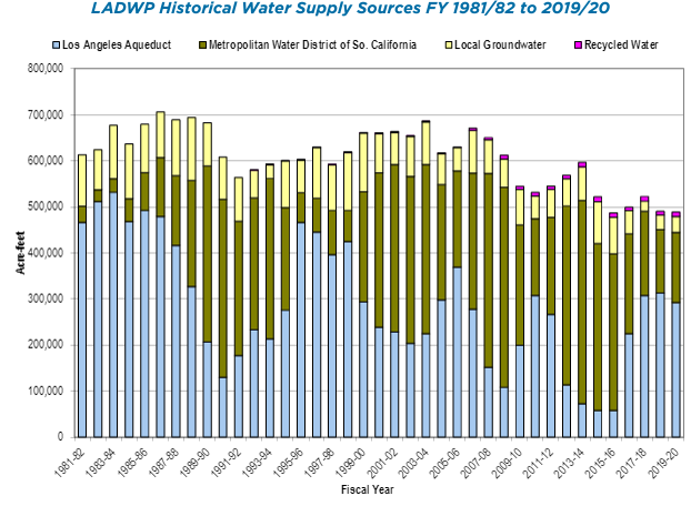
The trend in total water use for the City of Los Angeles (Figs. 3 and 4) is interesting because, although the population has increased significantly since 1970, average demand has remained relatively constant between 600 and 700 million acre-ft per year and has even decreased to around 500 million acre-feet in the past few years. This is a testimony to the effects of conservation and reuse because of source limitations (competing uses, drought) and rising costs. Economic downturns may also play a role. Certainly, one way to conserve water in LA is through limiting outdoor water use (car washing, landscaping/lawns). It is estimated that watering landscaping for individual homes is about 38% of total water use. Perhaps, like Las Vegas, LA should further encourage xeriscaping and graywater use for irrigating lawns and golf courses, but more on solutions in Module 8, Part 2 next week.
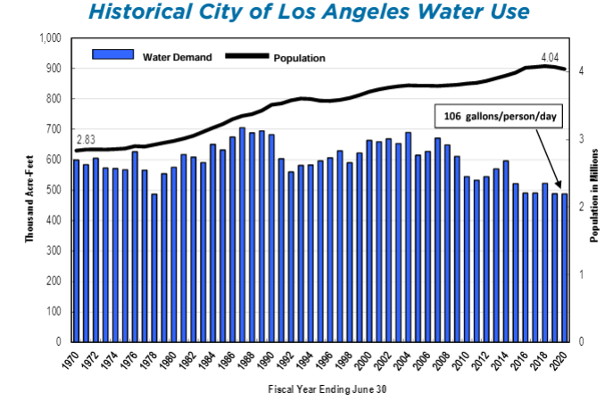
Cities In Peril: Las Vegas
Cities In Peril: Las Vegas
The Survival of Las Vegas

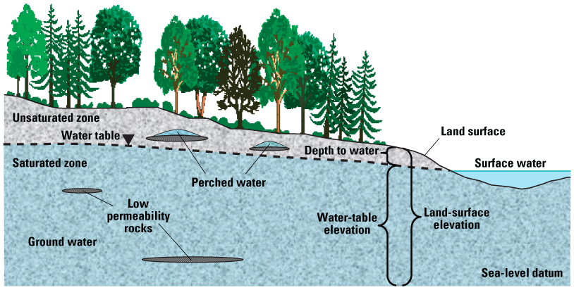
It’s hard to think about Las Vegas without images of stereotypical excess: gambling, bachelor(ette) parties, luxurious hotels, swimming pools, golf in the desert, posh fountains, celebrities, major music, and entertainment acts, and famous restaurateurs. On the one hand, it may seem incongruous that Las Vegas and the surrounding Clark County, which receive only 4 inches of rain per year on average and lie within one of the driest regions on Earth (Figure 5) (as discussed in Module 1), are also home to one of the fastest-growing populations in the U.S. (Figure 6; See also the interactive link in the caption below). On the other hand, it may be surprising that Las Vegas is among the most water-conscious cities in the nation, and as discussed below, despite rapid economic and population growth over the past two to three decades the city has managed to live within the limits of its relatively meager allocation of water from the Colorado River, the main water source for the region (see Colorado River Compact).


A Familiar History of Water and Population Growth
A Familiar History of Water and Population Growth
In the mid-1800s, early settlers named the area "Las Vegas", Spanish for "the meadows", because the Valley, fed by the Las Vegas Springs, was lush, grassy, and green. The springs yielded approximately 5,000 acre-feet of water per year. As you may recall, this is about the amount of water needed today to support 5,000 families of four, or a population totaling around 20,000. With a plentiful natural water supply, Las Vegas became a key stop and hub for the railroads: first the San Pedro, LA, & Salt Lake City Railroad, and later the Union Pacific.
In the early 1900s, private wells drilled into the valley-fill confined aquifer became commonplace to augment the spring flows, as residents tried to turn the valley into productive farmland. Many of the wells were artesian but were left uncapped (Figure 7). By 1912, the 1000 residents of Las Vegas withdrew about 22,000 acre-feet of water per year from the springs and aquifer. By 1930, a combination of several dry years and increasing demand led to overdraft conditions. In the meantime, the Colorado River Compact of 1922 allocated a small amount of Colorado River water to Southern Nevada (see Sidebar: CO River Compact). However, Las Vegas continued to rely principally on groundwater, and aside from some industrial uses, the Colorado allotment went largely unused until the 1940s. (Note that Hoover Dam, the primary infrastructure that allows surface water storage and withdrawal for Clark County, was not completed until 1936.)

With a steadily growing population and water demand, withdrawals greatly exceeded natural recharge and overdraft of the aquifer worsened. In an effort to reduce groundwater extraction, the Las Vegas Valley Water District was created in 1947, in part to begin using the Colorado River allotment. Despite these efforts, by 1960 the valley’s population had swelled to over 110,000, and almost 50,000 acre-feet of water were extracted from the aquifer annually. The natural springs dried up in 1962, and sustained overdraft led the potentiometric surface to drop by a few feet per year on average. The pattern continued through 1971 until the Southern Nevada Water System began delivery of Colorado River water from Lake Mead for municipal supply – 24 years after the water district was created.
With a plentiful supply (300,000 acre-feet per year) of Colorado River Water ready for delivery and distribution, population growth accelerated, reaching almost 700,000 by 1990 (Figure 8), and about 2 million by 2012. Coincident with the shift to water supply from Lake Mead in 1971, dependence on groundwater gradually started to decline (Figure9). As discussed in more detail below, managed (induced) recharge of the groundwater system using surplus Colorado River water was begun on a small scale in the late 1980s; this “banking” of water in wet years or times of surplus is viewed as one strategy to cope with water shortages.


Current Water Use and Sources
Current Water Use and Sources
Currently, about 90 percent of Southern Nevada’s water comes from Lake Mead (the Colorado River) (Figure 9); the rest comes from groundwater. Because of the very limited natural recharge to the aquifer system, and the fact that no other surface water is available, Las Vegas depends almost exclusively on the Colorado River to sustain its population and economy. The city is essentially at the mercy of the Colorado River. When the Colorado River Compact was signed in 1922, the allotment of 300,000 acre-feet per year was viewed as generous for the sparsely populated state. However, as may sound like a familiar story, with a rapidly growing economy, combined with good weather and apparently plentiful water, population growth rapidly exceeded most projections (see Figure 5).
Of the water delivered by the Southern Nevada Water Authority, it may be surprising to note that most (almost 60%) goes to residential use (Figure 10). Of this, a large fraction is used consumptively for watering lawns. As discussed in detail in The Big Thirst, incentive programs for removal of turf from parks, common areas, and residences is one strategy to reduce water use. Golf courses and resorts, which are often the stereotypical poster children for water “waste” in Las Vegas, use about 14% combined.
The pie chart shown in Figure 10 provides the first blueprint for conservation efforts and potential re-use, by identifying the key water uses in the district. Moreover, there is also a recognition that not all water uses are “equal”: some require clean water (i.e. residential uses, many industrial uses, medical), whereas others do not (golf courses, parks). As a result, reclaimed and partly treated water may be used for many needs. In Las Vegas, water re-use – essentially getting two uses of the same water - is one part of a diverse strategy to maximize the limited allocation of Colorado River water (additional detail on treatment facilities and pricing for reclaimed water are described on the water district’s website [121].
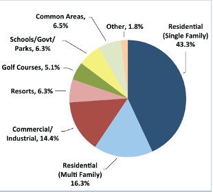
Dealing With Water Scarcity: A Diversified Portfolio
Dealing With Water Scarcity: A Diversified Portfolio
Due to a decades-long drought in the Colorado River system (see Sidebar: CO River Compact), the water level in Lake Mead has dropped by almost 170 feet since 2000 (Figure11). This corresponds to a decrease from ~25 million acre-feet of stored water to around 10 million acre-feet. If the lake water level drops to 1075 feet (as of June 2022, it is 1043 feet!), a federal shortage would be declared, triggering a reduction in Nevada and Arizona's allocations. In June of 2022, the U.S. Bureau of Reclamation decarded an emergency request for Colorado River states to reduce use by 2-4 million acre-feet within 18 months.To make matters worse, the two intakes in Lake Mead that withdraw water for Las Vegas cannot function if the lake level drops below 1050 feet (intake #1) or 1000 feet (intake #2). With the possibility of continued dry conditions, and because of their near sole dependence on Colorado River water, Las Vegas has developed a multi-pronged strategy to hedge against uncertainty due to future climate change coupled with likely increased demand due to growth and development in Clark County.

Conservation
Conservation
As you have read about in The Big Thirst: Dolphins in the Desert, Las Vegas has been aggressive in water conservation efforts. Part of these efforts focuses on simple reductions in household water use through education, regulation (i.e. watering restrictions), and incentivized removal of water-intensive landscaping. The city has also implemented GPS technology and pressure and acoustic sensors to monitor leaks in their pipelines to limit leaks and thus maintain high efficiency. As a result of these efforts, per capita, water use in Las Vegas has decreased substantially over the past 20 years or so, from over 340 gallons per day to less than 200 gallons (a 40% reduction!) (Figure 12). The SNWA has set a conservation target of 105 gallons per day fro 2035. As a result, Southern Nevada's total annual water use dropped by almost 90000 acre-feet (30 billion gallons) from 2002 to 2012, even as its population grew by 400,000.
Additionally, as noted above, Las Vegas treats wastewater for re-use, especially for applications that (a) don’t require high-quality water, like watering golf courses and parks; and (b) are consumptive. Re-use, incentivized by lower pricing, effectively allows the same water to be used twice, thus making the modest allotment of Colorado River water go further. Indeed, although Southern Nevada’s gross withdrawals from Lake Mead are almost 600,000 acre-feet per year (Figure 9), this is offset by the return of treated water to the Lake such that net withdrawals (consumptive use) remain at the 300,000 acre-feet limit.

New Sources: Tapping Groundwater
New Sources: Tapping Groundwater
Despite a history of overdraft in Las Vegas itself, Southern Nevada has recently turned its eyes back to the underground as an additional water source – but this time in sparsely populated valleys to the North and Northeast of Clark County (Figure13). The rationale for the SNWA’s “Groundwater Development Project” is that groundwater recharge is partly a function of the area over which infiltration occurs, so distributed withdrawals of groundwater from several large valleys fill aquifers outside of Las Vegas may be more sustainable than focused withdrawals from only the local aquifer system. Additionally, the targeted aquifers are in sparsely populated areas, with relatively small water demand.
Nonetheless, as you might imagine, there has been strong opposition to the plan from both environmental groups and ranchers and residents of these valleys, especially when considering past examples of the annexation of water rights for large cities (e.g., Los Angeles and the Owens Valley) and the negative outcomes for the local communities.

Water Banking
Water Banking
As another hedge against water shortage and climate change, the Southern Nevada Water Authority has entered into a series of “Water Banking” agreements with other the Lower Basin Colorado River states, Arizona and California. In these agreements, Nevada pays the other Colorado River water rights holders to store unused water in times of surplus by injecting it into aquifers. Nevada then receives credits for the stored water; if the water is needed, Nevada uses the credits to draw the equivalent water from Lake Mead, and in exchange, the “banker” withdraws the same amount from the aquifer. Although pumping is energy-intensive, groundwater banking does not require the construction of large reservoirs, and the water is not subject to large evaporative losses.
In its water banking agreement with Arizona, the SNWA paid $100 M initially and began making yearly $23 M payments in 2009 that will continue indefinitely. The agreement allows the SNWA to withdraw up to 40,000 acre-feet per year. In 2004, SNWA also began a water banking agreement with the Southern California Metropolitan Water District (the water district that serves L.A.) in which some of Nevada’s surplus Colorado River water is stored in an aquifer in Southern California. The agreement allows the SNWA to withdraw up to 30,000 acre-feet per year, provided that they give 6 months notice. Since 1987, Southern Nevada has also been banking its own surplus water – when available - in the valley’s aquifer for later use if needed. In Nevada, about 333,000 acre-feet have been stored through 2022, and in Arizona’s aquifer, the SNWA has stored 614,000 acre-feet of the Colorado River’s water through 2023.
Learning Checkpoint
1) How much is the cost of water banking per acre-foot? Do you think that’s worth it – and how does it compare to the cost of other water resources?
ANSWER:
2) Do you see a problem with the water banking approach to mitigating drought? Do you think it is sustainable in the long-term? Why or why not?
ANSWER:
The Third Straw
The Third Straw
In 2005, faced with the specter of prolonged drought and projected Lake Mead water level declines, the SNWA board of directors approved construction of the so-called “Third Straw”, a new $812 M intake from Lake Mead that would allow Southern Nevada to physically extract water from the lake at water levels as low as 1000 feet above sea level (Figure 14). Construction of the intake involves boring a 23-foot diameter tunnel through 3 miles of rock, with much of its length beneath one of the Earth’s largest man-made reservoirs!
The new intake will intersect the lake at 860 feet above sea level but will share a pumping station with intake #2, so will only be able to operate at water levels of 1000 feet (the same as for intake #2). The primary purpose of the third straw is to maintain overall system capacity if Lake Mead falls below the 1050 ft water level limit for operation of intake #1. It also will access the deepest parts of Lake Mead, where water quality is highest. The initial plan for the third intake included a separate pumping facility but was removed to cut costs. It is always possible that the $200 million pumping station and pipelines could be added in the future, though if the Lake Mead water level were to drop much below 1000 feet, there would be much bigger problems throughout the lower Colorado River basin.
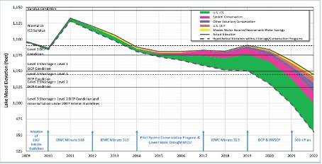
Figure 14 shows the elevation of Lake Mead on the y-axis versus the year on the x-axis including different water conservation projects. The important take home from this figure is that as we near 2022 we see that water levels drop. But as different conservation projects (in green, pink, purple, etc.) grow, the rate at which water levels drop decreases. In the time series, the thick dashed line represents the hypothetical elevation of Lake Mead due without conservation projects, while the solid black line represents the actual water level. Although water level is still dropping as of 2022, conservation efforts play a large role in stabilizing Lake Mead water levels.
The Colorado River Compact
The Colorado River Compact
The Colorado River flows almost 1500 km from its headwaters in Wyoming, Colorado, Utah, and New Mexico, through Nevada, Arizona, and California, before crossing the border to Mexico and flowing to the Gulf of California. It is the lifeblood of the American Southwest, serving almost 30 million people and enabling cities, industry, and irrigation-based agriculture to thrive in one of the direst climates on Earth (see Figure 1 in Module 8.2). The river also provides hydroelectric power that spurred much of the 20th-century development of the Southwestern U.S.
In 1922, these seven western states and the federal government negotiated an agreement, the Colorado River Compact (Figure 15) to allocate water rights on the river. First and foremost the compact partitioned water between Utah, New Mexico, Wyoming, and Colorado (the Upper Basin States) where most of its discharge originates as snowmelt); and Arizona, Nevada, and California (the Lower Basin States), where population growth and water demand were increasing rapidly (Figure 16).
The compact was borne in part out of the Upper Basin States’ unease that water projects and use of the river (e.g., by construction of the planned Hoover Dam) by the Lower Basin States at the time would, if interpreted through the lens of the doctrine of prior appropriations, impact their future claims to water from the river. The compact specifies that the Upper and Lower Basin would each have the rights to 7.5 million acre-feet of water per year. To accomplish this while recognizing that not all years would be the same, the delivery of 7.5 million acre-feet per year to the Lower Basin is evaluated based on a ten-year running average (i.e. the Upper Basin must deliver 75,000,000 acre-feet for any span of ten consecutive years). In fact, the primary purpose of Glen Canyon Dam, unlike Hoover Dam, which generates hydroelectric power and serves as the distributary dam for the Lower Basin States, is to serve as a large “capacitor” in the river system to help ensure that this agreement can be met. Later amendments to the agreement included the 1928 Boulder Canyon Project Act, the 1944 Mexican Water Treaty, and the 1948 Upper Basin Compact. In combination, these amendments spelled out the allocation of water between the individual states, and also allocated 1.5 million acre-feet for Mexico (Table 1).
Of course, the specification of an absolute amount of water to each of the states and Mexico has raised a few serious problems that remain contentious. First, the river is over-allocated. The 1920’s – coincidentally the time that the Compact was negotiated was an anomalously wet period with annual flows as high as ~20 million acre-feet (Figures17-18). In contrast, the long-term mean discharge of the river is about 15 million acre-feet, yet 16.5 million are allocated. Furthermore, the river flow is highly variable and based on historical data and tree ring reconstructions, it seems that decades-long dry periods with flows less than 13-14 million acre-feet may be common. Second, climate projections indicate that the region will become drier in the long-term, and some have suggested that we have already entered an era of steadily declining river flows along the Colorado. Fourth, improved understanding and renewed interest in the environmental impact of decades of dramatically reduced flow have spurred new pressures to allocate some discharge for the natural system. Finally, demand is likely to increase as populations in the region continue to grow, further stressing the already over-allocated river (Figure 18).


Colorado River Allocations (Million Acre-Feet per year, ten-year running average)
| Colorado | 3.9 |
|---|---|
| Utah | 1.7 |
| Wyoming | 1.0 |
| New Mexico | 0.85 |
| Nevada | .30 |
|---|---|
| Arizona | 2.85 |
| California | 4.4 |
| Mexico | 1.5 |
|---|---|
| Total | 16.5 |
Total of Colorado River Allocations(in Million Acre-Feet per year) = 16.5


Summary and Final Tasks
Summary and Final Tasks
Summary
In the first part of Module 8, you’ve learned about the water appropriation laws that have shaped access to water in much of the U.S. As you’ve seen, cities, especially in the arid American West, now must operate within the limits of these water appropriations, regardless of population or economic growth they have accommodated in recent decades. The tension between finite water allocation (i.e. from the CO River) and continued growth has motivated a diverse portfolio of strategies in place to cope with water scarcity and potential shortage. You are now well versed in these approaches, and should be able to describe them, and discuss the costs and benefits of each. In the second part of Module 8 (Module 8.2), we will build upon this knowledge and introduce another risk factor for water supply - that of climate change.
Reminder - Complete all of the Module 8.1 tasks!
You have reached the end of Module 8.1! Double-check the to-do list on the Module 8.1 Roadmap [129] to make sure you have completed all of the activities listed there before you begin Module 8.2.
References and Further Reading
The Big Thirst Chapters 5 and 7
Southern Nevada Water Authority 2015 Water Resource Plan [130]
Module 8.2: Cities in Peril: Future Climate Change, Population Growth, and Water Issues
Module 8.2: Cities in Peril: Future Climate Change, Population Growth, and Water Issues
Introduction
As has been discussed throughout this course, the relationship between humans and water resources has a long and complicated history. Water has played a central role in how and where human civilizations have developed. Proximity to high quality, reliable water sources provides a firm foundation for a thriving society. Societies that have established near unreliable or unpredictable water sources that may dry up during droughts and/or flood unexpectedly and uncontrollably) have struggled and occasionally suffered catastrophic losses. In other cases, societies have suffered more chronic problems with water quality. Advances in engineering have greatly improved accessibility and reliability of water resources, to an extent that is difficult to overstate. In some cases, however, a combination of highly effective engineering and risky (or ill-informed) decision-making has created some sketchy and unsustainable situations, as discussed in the first half of this module. What does the future hold? How, when and where might the legacy of our past decisions cause us severe problems in the future? What new problems might we anticipate as a result of climate change and population growth? Will technology save us? Or will more ecosystem-focused planning provide a more resilient water future for humans? How much of Earth’s water should humans feel entitled to? How much should be left for nature? These are some of the questions we’ll address in part 2 of this module.
Goals and Objectives
Goals and Objectives
Goals
- Describe the two-way relationship between water resources and human society
- Thoughtfully evaluate information and policy statements regarding the current and future predicted state of water resources
- Communicate scientific information in terms that can be understood by the general public
- Predict how human interaction with water on Earth is expected to change over the next 50 years
- Interpret graphical representations of scientific data
Learning Objectives
In completing this module, you will:
- Argue one of the many viewpoints on climate change.
- Identify the causes of global warming and climate change over the past ~250 years, including anthropogenic and natural influences.
- Assess whether mathematical models are a sound basis for making policy decisions.
- Evaluate the implications of climate change on future water resources for specific locations in the US.
- Devise a water plan for Phoenix, AZ, projecting forward from 1915
Water Use, Water Stress, and Population Growth
Water Use, Water Stress, and Population Growth
Module 1 discussed the who, how and where of water use throughout the US and the world. In the US and most industrialized countries, the dominant water uses are industry and agriculture. Domestic and municipal water use typically comprises only 15-30% of water use. In developing countries, per capita, water use tends to be lower in general, with a smaller proportion dedicated to industrial use and a larger proportion dedicated to domestic uses (see Module 1, Figures 8 and 9).
It is also useful to remember that we don’t actually see most of the water needed to sustain our daily activities. In the US, average per capita ‘direct’ use of water (domestic or municipal, for watering your yard, taking a shower, flushing the toilet, etc.) is 156 gallons per day, but the per capita ‘indirect’ use of water (including water used for energy production, manufacturing, food production, etc.) is 1230 gallons per day. So we really only ever see about 12% of the water that is used to sustain our quality of life. This ‘invisibility’ (as Charles Fishman refers to it in “The Big Thirst”) of our dependency on clean, reliable water is one of the challenges in planning for the future. Often we’re not even aware of what we stand to lose!
Population growth was also discussed in Module 1. The population is expected to grow by nearly a third of what it is today, to around 9.7 billion by 2050.For an engaging look at population increase in real-time, see the US Census Bureau Population Clock [131]. It is all the more concerning that some of the most rapid population growth in the world (India and Africa) is expected to occur in places that are already experiencing water stress. Add to this the legacies of past policies and infrastructure as well as future projections of climate change and it seems that we have a lot of work and planning to do!
Climate Change
Climate Change
What do and don’t we know about climate change?
Global warming and climate change: Both of these phrases have been used, often interchangeably, to discuss what is currently happening to our climate system. The term ‘global warming’ was coined by a Columbia University geochemist and climatologist by the name of Wallace ‘Wally’ Broecker in a 1975 Science article entitled “Climatic Change: Are we on the brink of a pronounced global warming?” Global warming, in the strict definition, refers to the observation that Earth’s average surface temperature is rising due to increased levels of greenhouse gases. The term ‘climate change’ includes global warming, but also considers the myriad other changes to Earth’s climate system that are caused by rising temperatures, including changes in precipitation and evaporation, movement of air currents (be they frontal systems or convective systems, hurricanes or a polar vortex), etc..
There is virtually no disagreement among climate scientists that both global warming and climate change are happening and is primarily due to human emissions of greenhouse gases. Broad agreement on these points among the science community is not because scientists tend to be an agreeable group. To the contrary, scientists are typically quite quick to disagree with one another and discuss their disagreements ad nauseam, in great detail and based on all available evidence, from empirical observations or theoretical physics and chemistry. Scientists also have large incentives to prove one another wrong. If, for example, a scientist was able to provide compelling evidence that increased greenhouse gases are not causing a systematic change in Earth’s climate system (or that evolution is not the driver of biodiversity, or that the Earth is not 4.6 billion years old), he or she would be famous as the likes of Galileo, Darwin or Einstein (all of whom toppled earlier scientific understanding), their work would be well funded (we would consequently have a lot of new questions that would need to be answered!), their book would be a best-seller, they would probably pick up a Nobel Prize and most notably, they would be interviewed by all of the most reputable talk show hosts. But no scientist has made such a compelling case. To the contrary, the case for significant climate change is compelling in both the empirical observations as well as the theoretical predictions. Those who proffer the opinion that climate change is not happening or is a hoax presumably do so out of sheer ignorance and/or because they have a financial incentive to believe (or to have others believe) that to be the case.
Distinct from the question of whether or not climate change is occurring, many questions remain regarding the effects of climate change on societies and economies. Certainly, there are positive effects. Warmer temperatures and increased carbon dioxide levels mean increased plant and crop productivity. Some places are expected to receive increased amounts of precipitation, potentially relieving water stress (though perhaps also increasing flood risk). Other places will most certainly not be so lucky and generally speaking, the risks and expected losses associated with climate change are expected to far outweigh the benefits. A comprehensive review of climate science and climate change is not possible within the scope of this course, but we will review a few of the key points as they relate to water, science, and society. We refer students to the most recent reports from the Intergovernmental Panel on Climate Change for more detailed and updated information.
Who Does Climate Science?
Who Does Climate Science?
Just about anyone could do climate science. Agencies, particularly in the US and Europe, have made an immense amount of weather and climate data available and with a modest amount of training and software anyone could perform rudimentary analyses of temperature or precipitation trends (e.g., see ncdc.noaa.gov or weather.gov or prism.oregonstate.edu). Of course, such analyses don’t answer all the questions. Tens of thousands of highly trained, independent scientists around the world collect and analyze climate data and develop models of global or regional climate change, which are typically tested using historical data and projected into the future. To provide a forum for discussion and debate that could be synthesized to represent our best understanding of climate change, the United Nations Environment Program (UNEP) and the World Meteorological Organization (WMO) established the Intergovernmental Panel on Climate Change (IPCC) in 1988. Thousands of scientists contribute data, analyses, and model results to the IPCC and provide critical peer review of any climate-related research, all on a volunteer basis. Six major assessment reports have been generated by IPCC, with the most recent report released in 2023.
What is Causing Global Warming?
What is Causing Global Warming?
While it is not our intent in this module to explore this question in detail, it is worth pointing out that many human activities clearly affect the climate system. Most notably, emissions of greenhouse gases, especially carbon dioxide and methane, are causing more heat to be trapped within Earth’s atmosphere. This effect, called the greenhouse effect, has been well understood since it was discovered by Svante Arrhenius in 1896. Figure 1 below, taken from the 2023 IPCC Working Group 1 Technical Summary shows the relative amount of heating or cooling of the climate system that can be attributed to the various factors that have changed between 1750 and 2019. The anthropogenic modifications to the climate system, enumerated in panel (a) of the figure, show the breakdown of radiative forcing. Anthropogenic forcing greatly outweighs the changes due to natural changes in solar irradiance. Panel (b) shows the effect each emitted component has on global surface temperature. The IPCC is quite careful to note the level of confidence associated with any given piece of knowledge, seen here with the black error bars of 5-95%. They are also transparent and are quick to point out when new understanding has significantly changed estimates or predictions, as has happened with our understanding of stratospheric water vapor, which was thought to be a significant contributor to warming in the Fourth IPCC Assessment Report (AR4, released in 2007), but has been found to be less significant.

Learning Checkpoint
According to Figure 1 above, total warming (i.e., positive radiative forcing) caused by human activities between 1750 and 2019 is equivalent to about:
(a) 0 W/m2
(b) 1 W/m2
(c) 2 W/m2
(d) 3 W/m2
(e)This cannot be determined from the graph.
ANSWER: (c) 2 W/m2
According to Figure 1, total warming (i.e., positive radiative forcing) caused by natural processes between 1750 and 2019 is equivalent to about:
(a) 1º C
(b) 1.5º C
(c) .5º C
(d) .25º W/m2
(e)This cannot be determined from the graph.
ANSWER: (a) 1º C
According to Figure 1, total warming (i.e., positive radiative forcing) caused by natural processes between 1750 and 2011 is equivalent to about:
According to Figure 1, the single biggest anthropogenic contributor to global warming is:
(a) Carbon dioxide
(b) Changes in surface albedo
(c) Aerosol emissions
(d) Methane
ANSWER: (a) Carbon dioxide
According to Figure 1, the biggest anthropogenic contributor to global cooling is:
(a) Greenhouse gas emissions
(b) Changes in surface albedo
(c) Aerosol emissions
(d) Tropospheric ozone emissions
ANSWER: (c) Aerosol emissions
What Are the Implications of Global Warming for Precipitation and Water Availability?
What Are the Implications of Global Warming for Precipitation and Water Availability?
So what does all this human-induced warming mean for the water cycle and water availability? Thinking back to module 2, you learned that warmer air can hold more water (i.e., warmer air has a higher saturation vapor pressure). Therefore it is reasonable to expect higher amounts of water vapor in the air. This is supported by observations that show a 3.5% increase in water vapor in the past 40 years as the climate has warmed about 0.5°C, with relative humidity remaining approximately constant.
Changes in precipitation are harder to measure (or predict) compared with changes in atmospheric water vapor content because of the immense temporal and spatial variability of precipitation. Nevertheless, patterns of precipitation change can readily be observed from historical records (Figure 2), with many areas seeing increases greater than 25 mm/year per decade (i.e., going from 300 mm/yr to 325 mm/yr over the course of a decade) and other places (particularly Africa and Southeast Asia) seeing decreases in precipitation at rates greater than 10 to 25 mm/year per decade. With increasing temperatures, it naturally follows that a greater proportion of precipitation would fall as rain, rather than snow, which has also been documented by the IPCC.
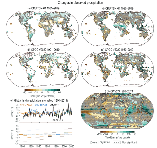
Learning Checkpoint
According to Figure 2, the two models (CRU and GPCC) indicate that, on average, precipitation throughout the conterminous US has ___________ from 1901 to 2019 (see left column of maps).
(a) increased
(b) decreased
(c) remained about the same
ANSWER: (a) increased
According to Figure 2, all three models indicate that, on average, precipitation throughout the conterminous US has ___________ from 1951 to 2019 (see right column of maps).
(a) increased in some areas and decreased in others
(b) decreased everywhere
(c) remained about the same
ANSWER: (a) increased in some areas and decreades in others. Note that the western US is seeing more dry conditions, and the eastern US is seeing more wet conditions.
Historical Precipitation Records and Climate Models
Historical Precipitation Records and Climate Models
What can the historical precipitation records and climate models tell us about the future?
But what can the historical precipitation records and climate models tell us about the future? Simulating future changes in precipitation patterns is one of the most difficult elements of climate modeling because precipitation and evaporation (there are feedbacks between the two so you have to model both) are driven by complex, non-linear processes. So climate models do not attempt to predict detailed representations of precipitation for any given location and climate models are generally not capable of predicting changes in precipitation intensity or frequency of extreme events, other than the likely sign (+ or -) of expected change. Nevertheless, all global climate models attempt to capture general trends in precipitation and considerable agreement exists among all the many competing models. In the broadest perspective, the IPCC makes the following important projections:
“Changes in the global water cycle in response to the warming over the 21st century will not be uniform. The contrast in precipitation between wet and dry regions and between wet and dry seasons will increase, although there may be regional exceptions.”
“Extreme precipitation events over most of the mid-latitude land masses and over wet tropical regions will very likely become more intense and more frequent by the end of this century, as global mean surface temperature increases (see Table SPM.1).”
“Globally, it is likely that the area encompassed by monsoon systems will increase over the 21st century. While monsoon winds are likely to weaken, monsoon precipitation is likely to intensify due to the increase in atmospheric moisture. Monsoon onset dates are likely to become earlier or not to change much. Monsoon retreat dates will likely be delayed, resulting in lengthening of the monsoon season in many regions.”
“There is high confidence that the El Niño-Southern Oscillation (ENSO) will remain the dominant mode of inter-annual variability in the tropical Pacific, with global effects in the 21st century. Due to the increase in moisture availability, ENSO related precipitation variability on regional scales will likely intensify. Natural variations of the amplitude and spatial pattern of ENSO are large and thus confidence in any specific projected change in ENSO and related regional phenomena for the 21st century remains low.”
Figure 3 shows the average temperature and precipitation results of many different competing models for two different scenarios, comparing observations in 1995-2014 to the projected time period 2081-2100. The figures are aggregates of a number of competing climate models from CMIP6. The two scenarios, called ‘Shared Socio-economic Pathways’ (SSPs) 2.6 and 8.5 are the two end-members of greenhouse gas emissions, with SSP 2.6 assuming that greenhouse gas emissions peak in 2010-2020 time period and decrease aggressively thereafter and RCP 8.5 assuming that greenhouse gas emissions increase throughout the 21st century. Notice that the warming (top plots) is not uniform throughout the world. The higher latitudes, especially in the northern hemisphere are expected to heat up considerably more than the temperate or tropical latitudes. We often hear numbers of the global average increase in temperature (estimated 1-2°C or 2-3.5°F by 2050), but this average value does not represent what is expected to happen at high latitudes. A 3-4°C (5-7°F) increase in the arctic, as indicated by SSP 2.6, represents a dramatic transformation of this ecosystem. A 8-10°C (18-21°F) increase in the arctic, as indicated by SSP 8.5, would represent a complete transformation of this ecosystem. What do you think would be the potential benefits and damages caused by such a transformation?
Changes in precipitation are also not expected to be uniform. In general, increases or decreases in precipitation are expected to be more drastic in the high greenhouse gas emission scenario (SSP 8.5) with some areas receiving 30-40% changes relative to 1995-2014. What ecosystem, economic or social changes might you expect to see as a result of a 30-40% increase or decrease in precipitation in the arctic? In Spain? In South Africa? In Chile?
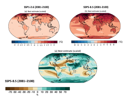
Projected Changes
Projected Changes
Figure 4 illustrates projected changes in other parts of the hydrological cycle during the time period 2081-2100 relative to 1986-2005 according to the high greenhouse gas emissions scenario (RCP 8.5). Note that the number of competing climate models represented for each panel of the figure is indicated by a number in the top right (range: 32-39 different models are averaged for each prediction). Future projections of water runoff or soil moisture are dependent on precipitation, which, as discussed earlier, is itself subject to substantial uncertainties. Nevertheless, it is worth considering what the variety of competing climate models have to say. For example, note the general (if slight) decrease in relative humidity over most land masses and a slight increase in relative humidity over the oceans (middle panel, left column). The middle panel in the right column shows changes in the difference between evaporation and precipitation with blue colors indicating a relatively wetter future (more precipitation relative to evaporation) and red colors indicating a relatively drier future (more evaporation than precipitation). The bottom panel in the left column predicts changes in surface water runoff. Note the significant declines in runoff throughout the southwestern US and southern Europe/northern Africa and parts of South America. This same trend is amplified in predictions of soil moisture, which is a primary control on plant growth (bottom panel, right column).

All Water Problems Are Local
All Water Problems Are Local
It is useful to know how climate change is likely to impact the water cycle at the global scale and IPCC reports represent our best understanding of those impacts over the next few decades to a century. But as we have discussed elsewhere, all water problems are local. In very few situations is it even feasible, let alone prudent, to transfer water long distances. Every place has its own set of challenges, institutional and infrastructure legacies, financial or other resource constraints, and concepts of social acceptability.
Generally speaking, places currently experiencing water stress or expecting to experience water stress in the foreseeable future have only a few basic options: a) have fewer people, b) force/incentivize people to use less water, c) increase storage and/or minimize losses within the system, d) reuse water, or e) get water from elsewhere. The capacity to cope with water stress (short or long-term) generally increases with wealth, though in wealthier countries more infrastructure is potentially at risk. As major population centers have already begun to struggle with water shortages it has become clear that massive investments in water technology and security infrastructure can allow wealthy nations to offset higher levels of water stress without remedying their underlying causes. Less wealthy nations, on the other hand, remain vulnerable and have fewer options in water development.
Salt Lake City
Salt Lake City
Salt Lake City: A case study in water development history and planning for the future
Salt Lake City (SLC) provides an interesting case study in terms of the history and future of water resource development. The first permanent settlers of Salt Lake Valley arrived in 1847 and immediately began diverting water from City Creek (northernmost of the four watersheds highlighted in blue in Figure 5). It is estimated that the early settlers hand-dug 1000 miles of ditches in the first few decades to distribute the water to agricultural fields, Salt Lake City and nearby settlements. By 1879 the population of Salt Lake County had grown to nearly 32,000 and the city authorized construction of the Jordan and Salt Lake City Canal, which was completed in 1882 with a capacity of 150 cubic feet per second, expected to provide enough water for 100,000 residents. The canal is still in use today. Several major dams were constructed as early as 1892 to 1907. Following a major water shortage in 1924, Mayor John Bowman proclaimed that ‘a city can never be greater than its water supply’ and initiated an ambitious water development program to supply reliable water for more than 400,000 residents. Several other large dams were constructed from the 1940s to as late as the 1990s to keep ahead of the rapidly growing population, but options for additional water storage via new reservoirs are now very limited.
Today Salt Lake City’s water supply is derived from several mountainous watersheds to the east of the city, in the Wasatch Front and western Uinta Mountains (Figure 5). About 50-60% of the water is derived from the four creeks just to the east of SLC (highlighted in blue), with the remaining portion delivered from the Weber, Provo, and Duchesne rivers via inter-basin transfers (tunnels, canals, and aqueducts shown as blue and white dashed lines in Figure 5) and extracted from groundwater. Around 70-80% of Salt Lake City’s water supply originates as snowmelt. Thus, the storage of water as snowpack, the timing of snowmelt, and water storage capacity within the system are all critical to ensuring reliable water supply.

Public utilities water use has remained relatively steady at 80,000 acre-feet of water per year since 1980. To put that number in perspective, imagine a tank of water an acre at its base and 80,000 feet (15 miles) tall, or the equivalent of a tank the size of Central Park in New York City flooded 100 feet deep. The fact that total public water use has remained steady over the past three decades is an impressive feat considering the population of Salt Lake County has nearly doubled from 620,000 in 1980 to nearly 1.1 million in 2014. Much of the Greater SLC area is populated by members of the Mormon religion, which has traditionally emphasized large families. More recently the size of families has decreased, but the population as a whole continues to grow.
Despite a growing population, total water use has started to decline in the past decade despite the fact that this time period includes three of the hottest summers on record, due to effective public education and water conservation campaigns (Figure 6).

Climate Change Further Complicates the Water Situation
Climate Change Further Complicates the Water Situation
Climate change further complicates Salt Lake City’s water situation. Peak supply from the four creeks typically occurs in early June and is expected to shift earlier in the year, to mid-May, in the coming decades. However, peak water demand typically does not occur until late July or early August. Hence the need for significant amounts of water storage. Temperature increases over the past few decades have already resulted in more winter precipitation falling as rain, rather than snow, thus reducing snowpack. The increased proportion of precipitation falling as rain, combined with an earlier snowmelt threaten the system’s ability to maintain adequate water supply through late summer. The total amount of water runoff is also expected to decrease as the climate warms. Every degree Fahrenheit of warming in the Salt Lake City region could mean a 1.8 to 6.5% drop in the annual flow of rivers that provide the city’s water supply. The semi-arid region is also known to experience frequent and sometimes prolonged drought. With a growing disparity in the timing and potentially the volume of water supply/demand, clearly, some changes are needed. Options currently being considered are further reductions in demand, additional water storage within the system, or extraction of groundwater.
Unfortunately, groundwater reserves are not in great shape. The shallow, unconfined aquifer underlying much of the valley is contaminated from uranium mine leachate, chloride, sulfate, iron, uranium, volatile organic compounds, and pesticides. Recent water quality testing from the shallow, unconfined aquifer found all samples to be below acceptable standards for drinking water. There is a deeper, confined aquifer that is in much better shape, with more than 80% of water meeting or exceeding water quality standards. However, excessive pumping of this aquifer has drawn down the water level by as much as 30-50 feet in places, from 2000-2022.


With the Great Salt Lake immediately adjacent to the city it might seem like desalination might be an option. Desalination, also called desalinization, is the process of removal of salt and other minerals to produce fresh water for consumption or irrigation. This is most commonly achieved by boiling water in a process called vacuum distillation or a process called reverse osmosis in which water is forced through a permeable membrane that strips out the salts. Either approach requires a considerable amount of energy and is therefore typically more expensive than most any other alternative. Considering that the Great Salt Lake is 3-8 times more saline than the ocean, this solution is currently not economically feasible to do on a large scale, though some desalination is currently done to treat partially saline groundwater.
People are, of course, not the only organisms that require access to clean and reliable freshwater. More than 75% of the wetlands in the state of Utah are found in Salt Lake Valley, which contains a wide variety of plant species, play an important role in regulating water quality, and provide habitat for a variety of birds, amphibians, and other animals. In addition, several threatened and endangered fish and bird species are dependent on the perennial flowing streams and rivers in the area. Water-stressed trees within the urban forest of the Greater SLC area have become more susceptible to disease. Lower precipitation in the mountains has increased the number and severity of wildfires.
Led by Mayor Ralph Becker, Salt Lake City has taken a proactive stance to adapt water resource management practices and mitigate the effects of climate change. Mitigation involves reducing the magnitude of the problem itself, whereas adaptation involves limiting one’s vulnerability to expected impacts. As part of the Water Conservation Master Plan, the city is attacking the problem from multiple angles. As a preventative measure, the city is purchasing and protecting large tracts of land in the watersheds that provide drinking water. SLC is also incorporating future climate scenarios into city and water development planning efforts, which is quite progressive for a state whose legislature passed a resolution in 2010 proclaiming that climate change was essentially a hoax.
The city is also attempting to bolster local resilience and reduce dependency on external sources of food, recently having passed several ordinances that promote local food production and community gardens. Also, the city is developing a water re-use program to provide water for city parks, golf courses, and the urban forest.
Recognizing that energy demand is a large and growing water use sector, the city is providing incentives for individuals and businesses to minimize the use of all forms of energy and invest in energy-efficient upgrades. Incentives are also in place for the use of solar energy (photovoltaic cells) and solar hot water heaters. The city has promoted net-zero building approaches (meaning that the amount of energy used by the building on an annual basis is roughly equal to the amount of renewable energy created on-site). And they have been willing to put their money where their mouth is…SLC’s Public Safety Building, completed in July 2013, is the first public safety building in the nation to be designed as a net-zero building and one of the first to meet the US Green Building Council’s LEED Platinum certification criteria. Climate change scenarios are being considered in many aspects of infrastructure planning, including building roads and sewers to handle higher runoff volumes and warmer temperatures. In recognition of the progressive direction, he has taken Salt Lake City Mayor Becker was appointed to President Obama’s climate adaptation task force in November 2013.
Module 9: Water and Politics
Module 9: Water and Politics
Overview
We have introduced some of the science and society issues in the first eight modules, and you have, by now, soaked up what you need to know to begin to formulate your own strong impressions of the major local and global issues and to come to some conclusions regarding possible solutions to them. In modules 9 and 10, we will expect more of you in the way of synthesis and solution.
The Pacific Institute has compiled a very cool, comprehensive list of water conflicts (Pacific Institute: The World's Water [135]) spanning recorded human history. Each event is accompanied by a brief account of the issue. Many of the earlier events chronicle the attempts to use water as an instrument of warfare—as a barrier to invasion, poisoning of water wells to deprive enemies of water, or destruction of water impoundments and irrigation systems, for example. World politics and creation of new nation-states in the twentieth century, however, created a different sort of conflict based on the need to divide crucial water resources between developing countries with burgeoning populations.
In this module, we will entertain several examples of international "water wars," referring to conflicts that occur within or between countries as the result of failed treaties and agreements, water supply interruptions, climate- or population growth-induced water shortages, and related issues. You are already familiar with an early and ongoing water conflict that involved the California-based antagonism between the City of Los Angeles and the Owens Valley beginning in the early 1900s (a conflict briefly entertained in Module 8.1 and related activities). Such episodes have a familiar cause—population growth, growing water shortage, acquisition of water, conflict, growth stimulated or supported by new water resources—creating a vicious cycle, as in the Los Angeles case.
Chapter 7 in "The Big Thirst" deals with the effects of climate change on rainfall in areas of already limited rain in Australia and suggests that this may be a problem for the long term. So-called "cli-fi," films, with apocalyptic climate-change scenarios at the heart of their plots, have become popular. No less than the Office of the Director of National Intelligence, which oversees all American intelligence agencies has released a report that suggests that climate change, and its influence on water availability, is a major near-future security issue. The United Nations World Food Program has estimated that 650 million people are living in areas where flood and drought can lead to food shortages and price spikes. For example, in East Africa, drought has led to warring among Somali clans for access to potable water. You should keep in mind the lessons of Module 8 Part 2 as we examine water "sharing" in this module—climate change enters into consideration of all of the examples herein, but is only explicitly mentioned in section called "The United States and Mexico—Sharing the Flow?" for the Colorado and Rio Grande River systems. A good example of internal issues related to recent climate change (prolonged drought) and poor government policy can be found here for Iran Washington Institute [136].
Goals and Objectives
Goals and Objectives
Goals
- Describe the two-way relationship between water resources and human society
- Synthesize data and information from multiple reliable sources
- Thoughtfully evaluate information and policy statements regarding the current and future predicted state of water resources
Learning Outcomes
In completing this lesson, you will:
- Analyze the political problems that arise when water supplies must be shared across borders
Sharing the Waters
Sharing the Waters
There are many examples of water disputes involving cross-boundary uses of shared resources. Three of these examples will be discussed in this section: The Nile River Conflict, The India-Bangladesh Ganges River Split, and The United States and Mexico— Sharing the Flow.
The Nile River "Conflict"
The Nile River "Conflict"
There are many examples of water disputes involving cross-boundary uses of shared resources. For example, in Module 5, we discussed the damming of the Nile River in Egypt and the Nile River's importance to development and water supply in Egypt. The construction of the Aswan Dam, which was authorized by a Nile Waters Agreement of 1959, was of little immediate concern to countries in the source regions of the Nile (Figs. 1 and 2), but guaranteed water rights allocated by earlier agreements were. Egypt initially negotiated the Nile Waters Agreement of 1929 with, what was then, a number of East African colonies of Britain (British as signatories). Through this agreement, Egypt was assigned rights to 48 billion cubic meters/year (bcm/y), including all dry-season flow (mainly from the White Nile), and Sudan, just to Egypt's south, was initially apportioned 4 bcm/y. In addition, Egypt had the right to veto upriver water projects. A later treaty, the so-called 1959 Nile Waters Agreement between Egypt and Sudan, allocated 55.5 bcm/y to Egypt and 18.5 bcm/y to Sudan—the total allocation was nearly 90% of the estimated average annual Nile River flow (84 bcm/y, mostly from the Blue Nile)! This was accomplished prior to independence for the other countries within the watershed and failed to include the monarchy of Ethiopia in negotiations. Interestingly, at the time of the agreement, the White Nile was considered, in error, the source of most of Nile water. Seasonal summer monsoonal rains in the Ethiopian Highlands are the source of much of the Nile waters, through the Blue Nile.


Conflicts have arisen, particularly since Ethiopia embarked on dam building. In 2010, six of the nine upstream countries (Ethiopia, Kenya, Uganda, Rwanda, Burundi, and Tanzania) signed a Cooperative Framework Agreement seeking more water shares from the Nile. Egypt and Sudan rejected the agreement because it challenged their historic water allocations but to no avail. A major dam on the Blue Nile, the Grand Renaissance Dam, is under construction near the Ethiopia-Sudan border. As of May 2016, the dam was about 70% complete, with a target date of 2017 to begin producing power (it is worth noting, however, that the original target date was 2015 - political conflict and construction issues have slowed progress on the dam). Sudan and Egypt are, understandably, concerned about what will occur to Nile flows as the reservoir behind this huge dam fills, but Ethiopia is hoping that the water and power supplied by this structure will boost their economy and help other surrounding nations as well. Ethiopia's population in 1950 was about 18.1 million, but by 2023 it had grown to 126.5 million (114 people/km2). In 1950, Egypt had a population of 21.5 million, and in 2023 there are 112.7 million (112 people/km2).One can see that demand for water must be increasing (source: United Nations Department of Economic and Social Affairs [137]), and that Ethiopia's growth has outstripped that of Egypt. However, Ethiopia has some other sources of water (estimated total river runoff at 122 bcm/y and additional large groundwater resources estimated at 6 bcm), whereas Egypt and Sudan must depend primarily on Nile water. However, Ethiopia has no storage capacity, hence the move to build a number of large dams. Will Egypt and Ethiopia go to war over Nile water? (see Analysis: Why Ethiopia and Egypt aren’t fighting a water war [138] for a perspective ).
The India-Bangladesh Ganges River Split
The India-Bangladesh Ganges River Split
Bangladesh achieved independence from Pakistan in 1971, following a short uprising. Bangladesh occupies the region of the original state of Bengal in India, which first became East Pakistan in 1947. India supported Bangladesh in the conflict with Pakistan.
The Ganges River (Fig. 3) was supposed to be shared in some way between India and Pakistan. It is fed by many tributaries (54) the largest of which is the Brahmaputra River that flows through Bangladesh, but most of the Ganges River Basin is in northeastern India. Summer monsoons deliver nearly 80 percent of annual rainfall for this region resulting in peak river flows from June-September. In an average year, it is estimated that 1200 billion m3 of precipitation falls in the Ganges catchment. Of this, nearly 500 billion m3 moves downriver. Dry season flows are much reduced.

India's proposal to construct the Farraka Barrage (a large dam) in West Bengal on the Ganges River right near the border led the two countries to meet over disputed water claims that originated in the 1950s following Bangladesh statehood. There was no resolution to the conflict and the dam was put into place by India without an agreement, with completion in 1975. The dam was constructed to divert some proportion of the Ganges flow into the Hooghly River (during the dry season in order to remove silt that was negatively affecting the port of Calcutta or Kolkata, Fig. 3). Although Bangladesh complained to the United Nations following severe water shortages in 1976, there was no significant resolution until 1996, when India and Bangladesh signed a 30-year treaty that provided for the partitioning of the flow of the Ganges River. The Ganges forms a border between the two countries for part of its course and continues to flow through Bangladesh to the Bay of Bengal. The 1996 treaty guaranteed India a flow of nearly 1000 m3/sec between January 1 and May 31. Much of the time Bangladesh receives less water than allocated by the treaty. India's population in 1950 was 376.3 million while the population of Bangladesh was only 37.9 million. Now India's population is 1.4 billion, (425 people/km2) and the Bangladesh population is 168.7 million (1136 people/km2). Bangladesh has a much greater population density but both countries have a great need for clean water and dependable water supply.
The United States and Mexico—Sharing the Flow?
The United States and Mexico—Sharing the Flow?
Most people in the U.S. probably don't think much about what water Mexico takes from the Colorado or the Rio Grande Rivers, which originate in the U.S. and flow along the U.S.-Mexico Border for some distance, and, in the case of the Colorado River, flow through Mexico to the sea (Fig. 4). Like the examples above (the Nile and Ganges Rivers), there are treaties that provide for sharing of the flow of these two North American rivers between the U.S. and Mexico. You have already read about the Colorado River Compact of 1922 (Module 8.1). In effect, the flow of the Colorado River is, on average, significantly less than the total amount apportioned to individual states in the watershed. The 1922 Colorado River Compact was vague about the amount of water that was to be supplied to Mexico. This was rectified in a 1944 Treaty that provided for 1.5 million acre-feet of water per year to flow to Mexico (about 10% of the average Colorado River flow).
The Colorado
The Colorado
Until the present, the U.S. has bypassed the requisite amount of water from the Colorado to Mexico every year, regardless of the total flow of the Colorado. Because of recent severe droughts in the southwestern U.S., however, a 5-year Agreement (Minute 319), signed in 2012, was brokered that allows the U.S. to reduce the amount of water shared with Mexico when Colorado River flow was much lower than normal. In that agreement, Mexico, which has little Colorado River storage capacity (only Morelos Dam and reservoir), will be allowed to store some of its surplus water in Lake Mead, behind Hoover Dam. In addition, the U.S. will help finance improvements to Mexico's water infrastructure ($21 million), which was badly damaged by an earthquake in 2010, and pledged to "reconnect" the Colorado River with the Gulf of California. The U.S. and Mexico committed to each supply 5,000 acre-feet of water a year to the delta. Accoring to the LA Times [139] in 2014, because of the Agreement, a "pulse flow" event occurred whereby, in March, nearly 105,000 acre-ft of water was released from Morelos Dam (Mexico) to restore (at least briefly) flow to the Colorado River Delta in the Gulf of California (Fig. 5). The intent was to begin to restore riparian ecosystems along the Colorado River in Mexico. However, in 2022, Mexico’s share of water was cut by 5% and nearly 7% in 2023. These pulse flows continue every spring and vegetation is beginning to thrive.

Of interest is the fact that there was more to the water allocation Treaty of 1944. In that Treaty, both the amount and quality of water allocated to Mexico were stipulated. The TDS of waters released to Mexico had to be below 1000 ppm. Alas, the salinity of Colorado River water behind Morelos Dam was typically greater than that because of evaporation and irrigation return flow (leached salt from arid-region agricultural soils in southern Arizona) So, the U.S. built desalinization plant in 1975 near Yuma to treat water to reduce TDS to maintain the agreed-upon values behind Morelos Dam in Mexico (actually partly in Arizona) according to stipulations made by the International Boundary and Waters Commission (IBWC) in 1973. However, the plant was never put into operation because of a period of high flow and lower salinity on the Colorado River. During the period 1973 to 2006, all the return flow from agricultural operations in the Yuma region (TDS=2500ppm; avg. nearly 125,000 acre-ft) was released to Mexico and flowed to the Ciénega de Santa Clara wetlands in Mexico (Fig. 6). This flow substantially contributed to the significant ecological development of the Ciénega as a wetland. In 2011, however, the desalination plant was tested for a year, and the flow of water to the Ciénega de Santa Clara was substantially reduced, with an associated increase in total dissolved solids (TDS>3200ppm). It remains to be seen whether the relatively low treatment volumes (30,000 acre-ft/y) of the desalination plant as configured are a benefit in light of concerns over the fate of the renewed Ciénega de Santa Clara ecosystem (over 30 yrs of runoff) and its endangered species (Yuma Clapper Rail and desert pupfish).


The Rio Grande
The Rio Grande
The Rio Grande River flows along the U.S. (Texas)-Mexico border for nearly 1,248 miles (2,008 km) including meanders. Although snowmelt from the San Juan Mountains of Colorado (Fig. 7) is a major source of water for the Rio Grande, runoff from northern Mexico also contributes to its flow. As in all arid to semiarid regions, the waters of the Rio Grande River are highly sought after and overallocated. And, as in the case of the Colorado River, the water division between the U.S. and Mexico is regulated by Treaty (see below).
Rio Grande River water is in demand because of the intense agriculture in New Mexico-Texas (Fig. 8) as well as in northern Mexico. This water supply deficit has been exacerbated by prolonged drought in the southwest. Figure 9 is a long-term record of flow of the Rio Grande River (at Otowi Bridge) reconstructed by tree ring records calibrated to more modern flows (see TreeFlow [140]). Note the frequent cycles of surfeit and drought, and the most recent steadily decreasing flow trend beginning about 1990.

In all, there are 15 dams on the Rio Grande River, many of them in New Mexico. Flows are significant until Elephant Butte Reservoir in New Mexico. El Paso, TX is 125 river miles downstream of Elephant Butte Reservoir and just upstream of the American Dam. Releases from Elephant Butte Reservoir control streamflow to El Paso. At American Dam, much of the flow in the Rio Grande is diverted for irrigation and municipal uses in Texas and Mexico. From the American Dam, the Rio Grande has little or no flow until joined by the Río Conchos about 300 miles downriver, which originates in the Sierra Madre Occidental in Mexico (see below). The Pecos River, a major U.S. tributary, joins the Rio Grande another 300 miles or so downriver near Langtry, TX (Fig. 7); the Pecos flow is also controlled by a dam upstream from its confluence with the Rio Grande. Further downriver, the flows in the Rio Grande River decrease significantly as the result of withdrawal for agricultural and municipal use in southwest Texas as well as the relatively low influx of water from tributaries. In Some years, the Rio Grande flow does not even make it to the sea near Brownsville, TX.


About 75% of water withdrawals from the Rio Grande River are in support of agriculture. Population growth has also been a factor, particularly in Mexico, where the population has nearly doubled since 2005, and nearly 6 million people depend on the Rio Grande River and related groundwater basins for drinking water. The U.S.-Mexico Treaty of 1848 established the international boundary, modified slightly by later "Conventions." The Treaty of 1944 between the two countries partitioned water from the Rio Grande River along the Texas-Mexico Border (as well as stipulating Colorado River flows to Mexico, see above), modified slightly by a 1970 Treaty, and authorized both countries to construct, operate, and maintain dams on the main channel of the Rio Grande. The International Boundary and Water Commission (IBWC) was assigned the task of dealing with water quality issues along the international border.
According to the Treaty of 1944, the U.S. is entitled to about one-third of the flow of the Rio Conchos from Mexico, which amounts to about 350,000 acre-ft/y on average. By the Treaty, Mexico is obligated to release 1.5 million acre-ft over a five-year period. During times of drought, it is difficult to meet the annual expectation, and, typically, Mexico releases more water in good rainfall-runoff years and conserves during drought periods, although at one point Mexico did not meet their obligation for nearly ten years. This pattern makes it difficult for agriculture in southwest Texas because water resources cannot be adequately predicted, and, in 2013, a controversy erupted between Texas and Mexico because of long-term drought that peaked in 2011 (Texas Observer: On the Border, a Struggle over Water [143]) --another example of the difficulties of sharing even major rivers.
Systems Thinking: Controls on Rio Grande River Flow to the Sea
Systems Thinking: Controls on Rio Grande River Flow to the Sea
Consider the water supplied by the Rio Grande River. In many years there is a trickle of water, or less, that reaches the sea. Why? Obviously, the water inputs are less than or equal to the outputs.
The Rio GrandActivate Your Learning
Construct a simple system diagram that represents the interplay between the "forces" that influence the flow of the Rio Grande River. Think about aspects of climate, population growth, and water demand as they influence Rio Grande River flow to the sea. Treat the Rio Grande flow/storage as a "reservoir" (total annual water availability in that system) and consider the most important inputs and outputs and the factors that drive them (refer to Module 1 for a background on systems thinking and systems diagrams). When you complete your system diagram on paper, click on the link to see what we expected you to include.
Click for answer.

Once you have studied the diagram, construct the "equations" for Annual Runoff and Annual Water Demand. Do the units match? How do you think this system would behave if the changes in inputs and outputs were large on a yearly basis?
Click for answer.
ANSWER:
Annual Runoff= Climate Variation x Annual Precipitation x Drainage Area
Annual Water Demand= Evaporation + (Water Use/Person x Percent Growth/y x Population)
If decreases in Runoff and increases in Water Demand were large (e.g. >1%/year) the Rio Grande would likely not flow to the sea. You could test this by putting realistic numbers into a model using these system relationships and running for several years.
Module 10: Solving the Water Crisis?
Module 10: Solving the Water Crisis?
Through the course of the semester and the first 9 modules of the class, you’ve learned about the science of water – including the distribution of fresh water; the demand for water and its relationship to geography, uses, population growth, and climate; and the physical principles that govern surface water and groundwater replenishment and movement. You’ve also considered some of the historical, political, ethical, and economic issues with water allocation and management, for example by considering the impacts of dams, or the annexation of water rights to support cities in arid regions.
In Module 10, the culmination of the course, you will explore potential solutions to the problems of water quantity and quality, especially in the face of population growth, increasing energy and food demands, and greater awareness of (and sensitivity to) the environmental impacts of water development. As major population centers, many of which are not ideally located with respect to water resources, continue to grow, we are faced with serious questions about sustainability: How can water supply and quality be assured, and balanced between the demands of irrigation and cities? Is there a technological panacea, or is a mixed portfolio of approaches required? Is it possible to hedge against climate change and predicted shifts in the timing and spatial distribution of precipitation? How can cost be managed, while minimizing the impact on the environment? Can diverse cultural and political entities work together to implement solutions, or deal with side effects, that cross state, and national boundaries?
Goals and Objectives
Goals and Objectives
Goals
- Describe the two-way relationship between water resources and human society
- Explain the distribution and dynamics of water at the surface and in the subsurface of the Earth
- Synthesize data and information from multiple reliable sources
- Communicate scientific information in terms that can be understood by the general public
- Identify strategies and best practices to decrease water stress and increase water quality
- Predict how the availability of and demand for water resources is expected to change over the next 50 years
Learning Objectives
By the end of this lesson, you should be able to:
- discuss the costs and benefits of desalination as a solution to water scarcity
- explain the benefits of water re-use
- describe the advantages and disadvantages of water optioning and water banking
- evaluate multiple approaches for safeguarding against water scarcity
- develop a portfolio of strategies for a water-poor urban area
Potential Solutions to Problems with Water Scarcity and Quality
Potential Solutions to Problems with Water Scarcity and Quality
In The Big Thirst, Charles Fishman repeatedly notes that while water problems are universal, they are fundamentally local and not global problems, in the sense that the issues are specific to a particular area, and excepting major water transfers, can most effectively be solved locally or regionally. Put another way, if you think back to Module 1, you’ll recall that if it were evenly distributed in time and space, the total precipitation that falls on Earth as part of the hydrologic cycle would be sufficient for water supply and dry land farming. The problem is not that there is not enough (or clean enough) water on the planet; it’s that the water does not fall when and where we need it. (see satirical article from the Onion [144])The fact that there is enough water globally does not help us all that much, because it is simply too expensive, impractical, and energy-intensive to move large volumes of water across oceans or between continents – though recent developments may challenge this mindset. Furthermore, the problems that face different areas are different: in Delhi, the major problems are related to water quality and infrastructure (i.e. Chapter 8 in The Big Thirst); in Las Vegas and Los Angeles, the problems are related to water scarcity and supply (Chapter 3); and in the Murray Basin or Perth, Australia, the problems are related to major shifts in supply and allocation in the face of changing climate (Chapter 7). Therefore, viable solutions are by nature local or regional – to obtain, manage, or treat water for a particular need and place. Potential Solutions to Problems with Water Scarcity and Quality
Here, we will briefly describe some of the most promising solutions on the horizon, many of which have been implemented as trials or in specific regions where the balance between demand and cost have made them feasible. We will also draw heavily upon readings from the textbook that you’ve completed for previous modules. For the assignment and activity linked to the module, we will ask you to develop a “portfolio” to secure future water supply for one of the population centers we’ve discussed in class (e.g., Las Vegas, Dubai, Los Angeles, etc…). This will require that you integrate much of what you’ve learned over the semester about precipitation patterns, surface water, and groundwater systems, water quality, water management and demand, cost, and infrastructure.
Seawater Desalination (SWRO)
Seawater Desalination (SWRO)
As you may remember from Module 1, the majority of Earth’s accessible water (i.e. not including a large amount of water trapped in minerals in the Earth’s interior!) is in the Oceans. In a sense, the Oceans would provide an unlimited supply of water, but of course, they are too salty to drink or use for most purposes. To use seawater for industrial, agricultural, or domestic/municipal supply, therefore, requires the separation of the water from the dissolved ions (mainly Na, Cl, Mg, SO4, Ca, and CO3). This can be accomplished in a variety of ways, but most commonly is done via either:
- Distillation, in which the water is forced to evaporate and then collected, leaving behind a concentrated brine, or
- Reverse osmosis, in which the water is forced through a semi-permeable membrane under pressure; the membrane physically excludes dissolved ions and other compounds, and only allows H2O molecules to pass (Figures 1 and 2).
Of these, reverse osmosis (or seawater reverse osmosis, SWRO) has emerged as the more efficient approach, especially when scaled to produce the millions of gallons per day or more needed to meet the demands of even modest population centers.
Of course, removing the salt from seawater requires energy – and money. For that reason, it has been a subject of intense research and engineering efforts, in order to reduce costs through increased scale, improved efficiency, pre-filtration, and improved materials (most importantly, advances in membrane materials that require less pressure to push the water through but still exclude dissolved ions). Early desalination plants were restricted to a relatively small scale, and mainly in desert areas (e.g., the Middle East), or to meet water quality requirements for the CO river treaty of 1944 (e.g., the Yuma desalination plant in Yuma, AZ, brought online in 1997). However, with improving efficiency, increasing demand, and perhaps spurred by drought, desalination is now emerging as one potential viable solution, at least in areas with access to the ocean, and the economic resources to construct and operate the plants.


Click for a text description
SWRO and Energy Costs
SWRO and Energy Costs
Technological advances, coupled with innovative approaches to reduce energy costs (i.e. by using solar, tidal, or ocean thermal energy) have helped to make SWRO a potential solution to water supply or hedge against climate change for large cities like Perth - rather than simply a novelty for wealthy countries. In the 1970s, SWRO costs hovered around $2.50/m3. Currently, costs for the most efficient plants are well below $1/m3, or between ~$1000-2000 per acre-foot (Figures 3 and 4). This is still more expensive than imported surface water or groundwater in most areas (these costs range from $400-1000/acre-foot, depending on location), but in the realm of viability for areas without those sources, or to augment limited supply. The total costs include everything from construction costs for the facility (amortized over its expected lifespan), land access, permitting for discharge and intakes, and operation & maintenance.
Despite its promise, it remains to be seen if SWRO will be a universal or large scale answer to water scarcity. In particular, key challenges include the (still relatively high) costs and associated energy demand; management of the environmental impact associated with intakes and disposal of the brine waste stream; delivery of SWRO water to regions away from the coast; and the up-scaling that would be necessary to meet demand for irrigation or industrial use.

Click to expand to provide more information
| Year | Power Consumption (kWh/m3) |
|---|---|
| 1970 | 16 |
| 1980 | 8 |
| 1990 | 5 |
| 2000 | ~3 |
| 2004 | 2 |
| 2008 | ~2 |

Click for a text description
| Year | Electric | Maintenance | Capex Charges | Total |
|---|---|---|---|---|
| 1982 | 0.7 | 0.2 | 0.6 | 1.5 |
| 1992 | 0.6 | 0.15 | 0.4 | 1.15 |
| 2002 | 0.3 | 0.1 | 0.3 | 0.7 |
| 2010 | 0.35 | 0.1 | 0.3 | 0.75 |
Activate Your Learning
Current water rates (cost for the consumer) in Las Vegas are $1.16 per 1000 gallons. From the data shown in Figure 4, calculate the typical cost of SWRO per 1000 gallons for 2010. Do the same for 1982. How much higher are SWRO costs than current water rates in Las Vegas for the two cases (i.e. are they double the cost? Triple? Ten times?). (Hint: You’ll need to convert between m3 and gallons: one m3 is equivalent to 264 gallons.
1982: $1.55/m3 x 1m3/264 gallons = $0.0059/gallon x 1000 gallons = $5.90/1000gal. This is about 5 times the cost of typical water delivery in Las Vegas.
2010: $0.93/m3 x 1m3/264 gallons = $0.0035/gallon x 1000 gallons = $3.50/1000gal. This is about 3 times the cost of typical water delivery.
Water Re-Use
Water Re-Use
As we’ve already seen in Module 8, one increasingly viable strategy to address limited water supply is that of treatment and re-use. This can take a variety of forms, including reclamation and re-use of wastewater for industrial or consumptive applications like golf courses or parks, or treatment of wastewater to meet drinking water standards and re-use for domestic/municipal supply. The former constitutes a major element of Las Vegas’s approach to maximizing their limited allocation of CO river water from Lake Mead. The latter is becoming increasingly – though not universally - accepted as a way to increase supply, and has been implemented in several areas, including Orange County and even at Penn State!
The Orange County Groundwater Replenishment System (GWRS) is one well-known case study of wastewater reclamation for municipal supply at a relatively large scale (Figures 5-7). The GWRS plant is a 70 million gallons/day facility (72,000 acre-feet/yr) and generates enough potable water for ~500,000 people. The facility also solves the secondary problem of managing effluent to the ocean because much of the wastewater that would otherwise be discharged offshore is captured and re-used. The facility takes advantage of proximity to the wastewater treatment facility to allow for low-cost and efficient “on-site” treatment and uses gravitational energy to transfer the water for treatment. The cost of the facility was subsidized by grants. With the subsidy, the cost of treated water is ~\$400-500/acre-foot; even without the subsidy, the cost is competitive with imported (CO River) water at ~\$800/acre-foot.


Two key advantages to reclamation and re-use are: (1) the supply is by definition local, in that it was used by the same people who would use it again, and has already been captured for treatment. This substantially reduces the need for infrastructure and conveyance, and thus is highly efficient and reduces cost; and (2) the total dissolved solids (TDS) in wastewater are much lower than in seawater, such that the energy and cost are low in comparison to SWRO (Figure 8).

Click here for a text description
| Type | kWh per million gallons (range) |
|---|---|
| Seawater desalination | 13000-17000 |
| Imported water (state water project/So. Cal) | 8000-15000 |
| Imported water (CO river aqueduct/So. Cal) | 6000 |
| Recycled water (membrane treatment) | 3000-8000 |
| Brackish water desalination | 1000-9000 |
| Imported Water (Northern California) | 0-3000 |
| Recycled water (tertiary treatment) | 1000-2000 |
| Local surface water | 0-1000 |
Another more local example is that of the Penn State “Living Filter”, which has been in operation since the early 1960s, and in full-scale operation since the mid-1980s. The treatment facility captures approximately 2.5 million gallons per day (the total water use on campus at the University, plus a small proportion of water used by residents of the nearby Borough of State College). This water is originally sourced from a fractured limestone aquifer that underlies the region. Rather than treating the wastewater and discharging it to local surface waters (Spring Creek), the water undergoes primary and secondary treatment, followed be de-nitrification and minimal chlorination to ensure that any (unlikely) remaining pathogens in the water are killed, and then spray application in the aquifer recharge area. After treatment, the biological oxygen demand has been reduced by 95-99%. The term “living filter” refers to the thick (>50-75 foot) soil column that overlies the aquifer; the combination of physical processes in the soil, natural degradation by exposure to soil acids and UV, and microbial activity effectively “filter” the treated wastewater to meet drinking water standards. In total, the system is almost 100% efficient in the re-use of extracted groundwater, with ~1 billion gallons of treated water per year recharged to the aquifer.
Of course, there are some obvious drawbacks to water re-use, though these are arguably mostly psychological and rooted in the so-called “Yuck Factor”. It is easy to forget that water is the ultimately reused product. The water in our rivers and oceans has certainly cycled through many organisms over the course of its history (think “dinosaur pee!”). The surface water that we think of as “clean” and which has historically been the dominant water supply for human consumption, hospitals, laundry, and other uses, is mixed with discharged treated wastewater from upstream communities. For that reason, we treat surface water before use. In this sense, why or how is directly treated wastewater any different? Likewise, rural domestic wells are often down-gradient of septic systems or leach fields, albeit a safe distance to allow natural degradation and filtration in the soils and aquifer system. Fundamentally, this raises the question of whether we would rather drink and do our laundry with water that was once our own wastewater, or somebody else’s.
Water Banking and Optioning of Water Rights
Water Banking and Optioning of Water Rights
As we covered in Module 8, one additional hedge against fluctuation in supply, and/or against climate change, is to purchase, trade, or bank water, either using one’s own allocated water in times of surplus or through the purchase of someone else’s unused water rights in a given time period. For example, Las Vegas has adopted this strategy to provide alternate sources in times of severe water shortage, through agreements with Arizona and California. These agreements are one means to transfer water, either actually or virtually, from areas where it is available (in surplus or actively stored in aquifers) to those where it is needed.
More sophisticated arrangements have also been explored, in which water is treated as a commodity and with prices determined by demand. One example of this is described in the High Country News piece "LA Bets on The Farm [151]". The basic concept is that the MWD of Los Angeles pays farmers with water rights for irrigation to fallow some portion of their land. Because, at least currently, there is no shortage of food, the exchange works: LA gains an additional water supply, and the farmers or irrigation districts make a bit of money (without having to take on any risk associated with growing crops, commodity prices, or the like). A more recent iteration of the agreement provides both parties with additional flexibility to account for unpredictable precipitation patterns and water supply, whereby the MWD purchases “options” to the water rights for $10/acre-foot. By March of that particular year, the MWD must decide whether they will take the water or not. If they do, they pay an additional $90/acre-foot (enough that the irrigation districts make some money); if not, there’s still time to plant crops, and the irrigation district keeps the option fee.
At their core, these approaches use the market to define the pricing of water and to shape the terms of agreements that will be mutually beneficial. In part, they work because the amount of water needed for irrigation far exceeds that for municipal or domestic uses (see Module 1). And in part, they work because the irrigation districts receive water that has been heavily subsidized, largely through public investment in major infrastructure that underlies the water systems. Ultimately, however, it is not clear that the exchange or purchase of water rights will really work in the face of severe drought, major climate changes, or continued increases in demand. After all, these strategies are essentially a form of regional water re-allocation or transfer – but in a zero-sum game, they can only work if there is enough surface water or groundwater to be had.
Recognition that these strategies may ameliorate shortages and can serve as a valuable hedge against variability in supply, but are unlikely to fully solve problems of water scarcity if we insist on continued development in water-poor regions, has led to large-scale proposals to transfer water or exchange water rights over great distances and across borders. For example, as discussed briefly in Module 8.1, and in Chapter 3 of The Big Thirst, Las Vegas has begun to explore distant sources of water. These include groundwater in Central and Northern Nevada (a project currently underway), as well as proposed exchanges in which Las Vegas would bankroll desalination facilities in Coastal California, and trade the “new” supply of desalinated water for withdrawal of the same amount from Lake Mead. As described in the next section, the basic fact that there is water available if one reaches far enough – and is willing to pay for it - has led to all manner of proposals to move water across oceans and continents. To an extent, this calls into question Fishman’s assertion that all water problems and their solutions are “local”.
Activate Your Learning
Explain (~100 words) why water banking or optioning is not a viable long-term solution to water scarcity in the case of prolonged water shortage related to sustained severe drought or climate change.
Answer/talking points: Should note that these approaches are no more than water trades, either with other end-users at the current time, or for future water access or rights. These strategies, therefore redistribute or reallocate water to meet the greatest or most severe demand. But if there is simply not enough water to meet demand on a long-term basis, reallocation cannot solve the problem.
Distant Sources
Distant Sources
If you have ever carried your water on a camping or backpacking trip, you know first hand that water is heavy, and therefore that transport is costly and energy-intensive (that’s why there is a market for water filters and iodine tablets!). For example, almost 20% of electricity in California is used for the water-related activity, and much of that to move water across the state. Despite the high energy and economic cost to transfer large volumes of water, it remains the only – and ultimate – hedge against uncertain supply. As you’ve heard from Marc Reisner and George Miller in the Cadillac Desert films we’ve watched, the idea behind many ambitious water proposed water projects in the Western US, many of which never reached fruition, was to “go where there was so much water, you’d never run out”, and construct “pipelines beyond the wildest imagination”. Patricia Mulroy has even suggested that water transfers from the Great Lakes to the American Southwest should be considered in order to serve the greatest good; water rights and export form the Great Lakes watershed is, not surprisingly, a controversial topic.
In most instances, large-scale water transfers over huge distances by pipeline or tanker are simply too expensive to make sense, or there is too much political resistance. As one extreme example, in the early 1990s, Walter Hickel (then governor of Alaska) and California congressmen Edward Roybal and George Brown requested a feasibility investigation for a pipeline that would bring water from Alaska to California through a subsea pipeline (Figure 9). The committee estimated that the cost of water transfer would be between $3000-4000 per acre-foot, or approximately triple to quadruple the cost of SWRO desalination. In the same report, the committee assessed other sources of water for California and noted that bringing water in by tanker would cost $1,500-2,000 per acre-foot for contracts of at least 30,000 acre-feet.

In other cases, the economics are not as prohibitive. For example, water is routinely transferred within California, or between Western States (e.g. Colorado River water transferred to Southern CA in the All American Canal) over distances of hundreds or even over a thousand km. This so-called “imported water” is the basis for the cost comparison of alternative supplies. At a yet larger scale, China has recently undertaken the world’s largest water transfer project, the South-to-North Water Diversion Project (or SNWDP). The main driver for the water project is that precipitation, and thus water resources, are very unevenly distributed across China (Figure 10) – and water-scarce provinces account for over 40% of the GDP. At the same time, almost a third of the population (300 million people) have access only to contaminated water – largely because of insufficient clean water supply and/or limited surface water flows that do not flush pollutants from the channel (as discussed in Module 5 – sidebar on the Three Gorges Dam).
The SNWDP will move almost 45 billion m3 of water per year (36 million acre-feet, or ~3 times the Colorado River’s flow), over distances of almost 4500 km. Although the financial benefits seemingly outweigh the costs – and hence the project is moving forward – major drawbacks are inevitable. For example, such a large water transfer is likely to have major impacts on river systems, in terms of changes in flow, sediment transport, and flushing; relocation of people along the route; construction across archeological and religious sites; and environmental impacts on wetlands that may disappear and endangerment of species that have adapted to the natural river flow regime (sound familiar? think back to Modules 3, 4, and 5!)

.png#mediaviewer/File:China_average_annual_precipitation_(en).png)