Module 3: Rivers and Watersheds
Module 3: Rivers and Watersheds
Overview
In this module, we will investigate the processes by which precipitation accumulates in, moves through, and is transported out of a landscape. We will especially focus on flow of water in streams and rivers, including how these important features form and change over time. The goals of the module are to develop an understanding of the water cycle at the watershed scale, as well as to explore the variety of rivers that exist on Earth’s surface, develop an understanding of how those rivers change over time and learn how to measure the amount of water transported by a stream or river. As part of this, you’ll come to understand how water is conveyed to a river, and become familiar with terms such as flow duration, sediment transport, channel and floodplain morphology, and stream and watershed restoration.
Goals and Objectives
Goals and Objectives
Goals
- Explain the distribution and dynamics of water at the surface and in the subsurface of the Earth
- Synthesize data and information from multiple reliable sources
- Interpret graphical representations of scientific data
Learning Objectives
In completing this module, you will:
- Identify and describe the processes by which precipitation accumulates, moves through, and is transported out of a watershed
- Describe the physical differences between terrestrial and stream systems
- Qualitatively evaluate stream gage data
- Visually identify various common channel morphologies in Google Earth
- Describe physical characteristics of a river channel, including stream order, number of channels, and sinuosity
- Analyze how topography influences water movement over land
Water Moves Through the Landscape
Water Moves Through the Landscape
The most obvious way water moves through a landscape is via stream and river channels. There is no formal definition to distinguish between brooks, creeks, streams, and rivers, but generally speaking, the former terms refer to smaller waterways and the latter refer to larger waterways. The terms stream and river are often used interchangeably. There are over 3.5 million miles (5.6 million kilometers) of streams and rivers in the US. If all the streams and rivers throughout the US were lined up one after the next, they would extend the distance from Earth to the moon and back...seven times! That is an incredible length of streams to be monitored, protected, regulated, and (occasionally) repaired by federal, state and local agencies, as well as industry and non-profit organizations and individuals. In addition, streams sculpt much of the surface of the Earth, forming a multitude of beautiful patterns and awe-inspiring features, as shown in Figure 1.

Channel Networks and Watersheds
Channel Networks and Watersheds
Streams naturally assemble themselves into surprisingly well-organized (quasi-fractal) networks. Figure 2 shows a typical channel network where many small streams converge to make progressively larger streams. The smallest streams in the network, which have no other streams flowing into them, are referred to as first order streams. When two first order streams meet, a second order stream is formed. When two second order streams meet, they form a third order stream, and so on. According to this conventional stream ordering system, first developed by Horton (1945) and refined by Strahler (1957), when a smaller order stream (e.g., first order) meets a larger order stream (e.g., second order), the resulting stream retains the order of the larger stream (in this case, second order).
Each stream has a watershed, also known as a ‘river basin’ or ‘catchment’ because it is the land that ‘catches’ precipitation and funnels it towards the stream. The watersheds of two first order streams are outlined with grey dashed lines in Figure 2. The watershed of a second order stream is outlined in black dashed lines and encompasses the two first order watersheds. The solid black outline in Figure 2 shows the watershed boundary for the fourth order watershed, which encompasses all other watersheds nested within it. The right side of Figure 2 shows the Mississippi River watershed highlighted in green, with the Missouri River watershed nested within it, highlighted in orange. By the time the Mississippi River reaches New Orleans, it is a tenth order stream (though only a few of its largest tributaries are shown in Figure 2), and drains more than one-third of the contiguous US.
The concept of connectivity between rivers and their watersheds will come up again towards the end of this module in the context of restoration. If a particular stretch of stream is impaired for one function or another (e.g., fish habitat has been degraded), in some cases it makes sense to ‘fix’ that specific stretch of river, while in other cases the impairment is simply a symptom of problems higher up in the watershed, so the ‘fix’ may need to be applied at that location in the watershed before human intervention or natural processes can begin to repair the impaired stream. Such is the way that watersheds and streams are connected.

Watersheds are Complex Systems
Watersheds are Complex Systems
When you look around, you see that the world is full of systems…assemblages or combinations of things that form a functional unit. Some systems are human-made, others are made by nature. Some systems are simple, meaning the way they work is straightforward and the outputs from the system are easily predictable. Other systems are complex, meaning they often have many parts that interact, often in non-linear ways, making the outputs from those systems more difficult to predict.
For example, a coffee maker is a pretty simple system. You put in 8 cups of water and two cups of coffee grounds and (assuming you put them in the right places), you turn the machine on and get ~8 cups of coffee. If you change the amounts of either of the inputs, it is pretty easy to predict the impacts on the coffee you brew.
Watersheds are not such a simple system. They are incredibly complex. One example can be seen in how the relationship between rainfall and runoff changes throughout the year. In a simple system, you would expect a constant relationship between incoming rainfall and outgoing flow. For example, a 1-inch rain event should translate to a stormflow hydrograph that might last 2 days and peak at 1000 cfs. But this isn’t what we see. Figure 3 shows streamflow (blue line, values on the left axis) and precipitation (orange bars, values on the right axis) from March through September 2008 for the Maple River near Rapidan, Minnesota. Precipitation is relatively evenly distributed throughout the year. As you can see, in April and May, rainfall events that are 0.5 to 1 inch result in relatively high flows (1000 to 1500 cfs). However, in July, August, and September, similar rainfall events hardly elicit any flow response whatsoever! Why do we see such non-linear behavior?

Activate Your Learning
The Maple River example above is a relatively extreme example of changes in rainfall-runoff relationships because soils are relatively wet (and therefore can’t absorb much of the incoming rainfall) in the spring and there is very little vegetation to intercept or evapotranspire water (the watershed is covered in row crops that don’t grow much before mid-June). In contrast, the row crops are in full effect by mid-summer and early fall and therefore they dry out the soil, intercept some incoming rainfall and evapotranspire most of the rest of the incoming rainfall…so it never gets to the channel! But similar phenomena can be seen in other watersheds. Find precipitation and streamflow data for a watershed of interest to you (from the USGS website, NRCS SNOTEL website, or NWS website). Plot them as shown in Figure 3. How well does flow correlate with precipitation? Are there seasonal differences? Differences from year to year?
Watersheds comprise many interacting parts. Figure 4 (top panel) is one way to represent various ‘parts’ that might be considered to comprise the watershed. While this is clearly a very simple view of this complex system, it is useful to take a “crude look at the whole”, a term coined by Nobel Prize-winning Physicist Murray Gell-Mann, as a starting point. When one component of the system is systematically changed, it may have direct as well as indirect impacts that propagate through the system. For example, changes in precipitation, snowmelt regime, or water storage may change streamflow. This altered streamflow has direct effects on river channel morphology, sediment transport, riparian vegetation, water quality, nutrient processing, and biodiversity, as indicated by the yellow arrows in the middle panel of Figure 4. But there are other interactions within the system, feedbacks that are indicated by purple arrows in the bottom panel of Figure 4. So to predict impacts of the changes in flow on aquatic biodiversity you would have to take into account not only the direct effects (yellow arrow between flow and aquatic biodiversity, but also the indirect effects associated with changes in channel morphology. This concept is also relevant in the context of watershed ‘restoration’. If a particular stretch of stream is impaired for one function or another (e.g., fish habitat has been degraded), in some cases it makes sense to ‘fix’ that specific stretch of river, while in other cases the impairment is simply a symptom of problems higher up in the watershed, so the ‘fix’ may need to be applied at that distant location in the watershed before human intervention or natural processes can begin to repair the impaired stretch of stream.
These notions of complex feedbacks and cascading effects greatly complicate the process of predicting what impacts human activities or natural disturbances within a watershed might have downstream. We’ll come back to this theme of system dynamics and complexity throughout the course.


Streams
Streams
Streams are the most obvious way that water is moved through a watershed because we see them all over. But there are many other means by which water moves, as discussed in module 2. Figure 5 illustrates the various stocks (places were water is stored, even if only temporarily) and fluxes (mechanisms by which water moves) of water that may exist within any given watershed. For example, one raindrop might fall onto vegetation (called interception) and subsequently be evaporated back up into the atmosphere. Another raindrop might fall onto the soil surface and then runoff the surface into the stream channel or it might infiltrate down into the soil. Once in the soil, the water might further percolate down into the groundwater, where the soil or rock is saturated with water. Alternatively, once in the soil, the water might travel downhill within the soil and runoff into the stream or it might be taken up by vegetation and transpired back into the atmosphere. Estimating and predicting which, and to what extent, water travels through these pathways is an active field of hydrologic research and is also vitally important for environmental management and policymaking, as certain pathways may be more or less prone to filtering or polluting water along its journey to the place where you might want to use it for drinking, irrigating, fishing, swimming or the myriad other purposes for which we need water.

River Flow Changes Over Time
River Flow Changes Over Time
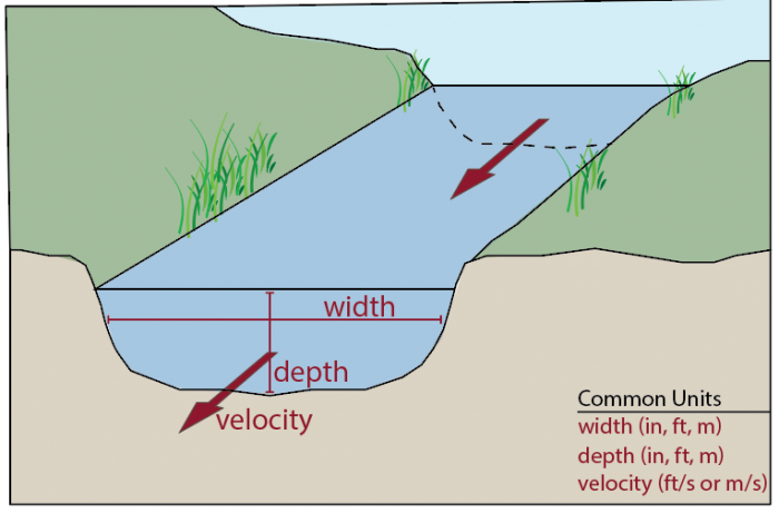
The amount of water moving down a river at a given time and place is referred to as its discharge, or flow, and is measured as a volume of water per unit time, typically cubic feet per second or cubic meters per second. The discharge at any given point in a river can be calculated as the product of the width (in ft or m) times the average depth (in ft or m) times average velocity (in ft/s or m/s).
The vast majority of rivers are known to exhibit considerable variability in flow over time because inputs from the watershed, in the form of rain events, snowmelt, groundwater seepage, etc., vary over time. Some rivers respond quickly to rainfall runoff or snowmelt, while others respond more slowly depending on the size of the watershed, steepness of the hillslopes, the ability of the soils to (at least temporarily) absorb and retain water, and the amount of storage in lakes and wetlands.
Video: How to Measure a River (8:35)
Hydrograph
Hydrograph
A hydrograph is a graph of discharge over time. The time period shown could be short, for example, the flow resulting from an individual rain storm, or it could be long, for example, a continuous record of flow over many decades. While numerous federal and state agencies, corporations, and individuals monitor discharge in streams throughout the country, the US Geological Survey is the chief entity charged with monitoring streamflow, maintaining over 9,000 stream gages, most of which record water discharge in 15 minute intervals and many of which also include water quality data. Visit the USGS Water Resource webpage (water.usgs.gov) and peruse the wealth of information compiled to assess water resources. Exercises utilizing these data are included below in module 3 as well as module 4.
The Figure 4 shows example hydrographs from the Logan River, near Logan, Utah for two different water years (2006 and 2012). The water year begins October 1 and ends September 30. Hydrologists often prefer to conduct analyses based on the water year rather than the calendar year to facilitate comparison of incoming precipitation and outgoing streamflow, and specifically to ensure that snow delivered in October, November, or December is accounted for in the same time period that it is likely to melt, which may be in spring or summer of the following calendar year.
The Logan River hydrograph shows a long (about 5 month) prominent peak in discharge, primarily driven by snowmelt, with many other smaller peaks superimposed (from accelerated snowmelt during warm periods or rain events). The hydrograph of the Logan River over a 50 year time period (Figure 6) shows the prominent peak from snowmelt each year, but provides little information about the smaller scale variability that is visible on the annual timescale. Note the non-linear y-axis of the plots. Such axes can be useful for visualizing detail in both high and low flow conditions, whereas the detail in low flows would not be visible on (typical) linear axes. The apparent shift in low flows circa 1970 on the Logan River was caused by removal of a water diversion upstream from the gauge. Note that there is a considerable amount of ‘noise’ (i.e., variability) in streamflow over the past 50 years. This variability is not random, but rather has some ‘structure’ to it, some of which is visibly obvious (annual peaks) and other portions that can only be quantified using advanced analytical or statistical techniques, which are beyond the scope of this course, but currently represent a vibrant facet of hydrologic research.


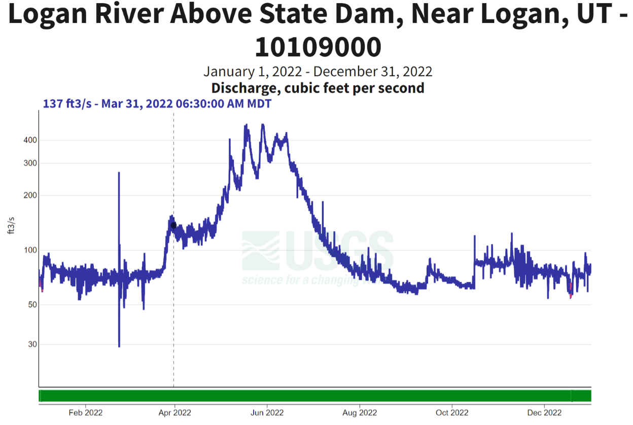
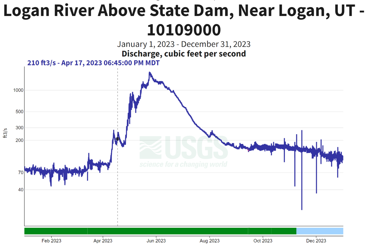
Examples of Logan River Hydrographs 2022-2023
River Flow Regimes
River Flow Regimes
The temporal patterns of high and low flows are referred to collectively as a river’s flow regime. The flow regime plays a key role in regulating geomorphic processes that shape river channels and floodplains, ecological processes that govern the life history of aquatic organisms, and is a major determinant of the biodiversity found in river ecosystems. There are five components that characterize the flow regime:
- Magnitude: the total amount of flow at any given time
- Frequency: how often flow exceeds or is below a given magnitude
- Duration: how long flow exceeds or is below a given magnitude
- Predictability: regularity of occurrence of different flow events
- Rate of change or flashiness: how quickly flow changes from one magnitude to another
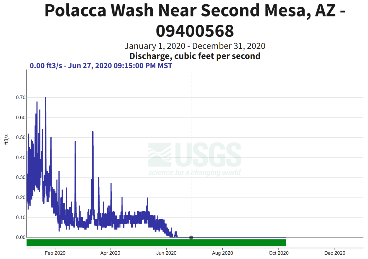
River in regions with similar climate, geology, and topography tend to have similar flow regimes. For example, rivers draining high mountains, such as the Logan River, tend to have relatively infrequent, high magnitude, long duration, and predictable flood events that have a slow rate of change (Figure 6 on the previous page). Rivers in many tropical climates have similar flow regime characteristics as mountain rivers, due to predictable rainy and dry seasons. In contrast, rivers in arid regions are often characterized by high magnitude, short duration floods of low predictability and high flashiness (e.g., Figure 11 on the next page).
Within regions of similar climate, local factors such as soil type, soil depth, vegetation cover, and watershed size influence the natural flow regime. For example, watersheds with deep, permeable soils will be able to absorb more precipitation than watersheds with thin, impermeable soils, and will thus tend to have less flashy floods of lower magnitude and longer duration. Large rivers tend to be less flashy than small streams, which respond more quickly to individual precipitation events. Thus, natural flow regimes can be somewhat variable between nearby watersheds. Also, although general patterns in flow regime can be determined from watershed characteristics, yearly variation in precipitation patterns means that many years of flow monitoring will be required to fully characterize the flow regime of individual rivers.
Temporary vs. Perennial Streams
Temporary vs. Perennial Streams
Most large rivers are perennial, meaning they maintain flow throughout the year. However, many headwater streams or streams in arid regions sometimes run dry. A stream is considered temporary if surface flow ceases during dry periods. Temporary streams are often classified further as intermittent and ephemeral. An intermittent stream becomes seasonally dry when the groundwater table drops below the elevation of the streambed during dry periods. A spatially intermittent stream may maintain flow over some sections or surface water in deep pools even during dry periods due to locally elevated water tables or perched aquifers. An ephemeral stream only flows in direct response to precipitation such as thunderstorms. Thus, the flow variability of an intermittent stream is much more predictable than in an ephemeral stream.

In many parts of the world, such as the desert southwest, temporary streams may comprise a majority of the river network, >80% in some areas. However, even in wet regions, temporary streams at the head of river networks can account for >50% of the total stream network. Thus, river networks can be considered dynamic systems, with total miles of surface flow expanding and contracting in response to precipitation events.

Why would we still call a channel that goes dry for much of the year a stream? In other words, how can we distinguish between a temporary stream and an upland terrestrial ecosystem? In short, a stream has characteristic hydrological, geomorphological, and ecological processes. However, as with many topics in environmental science, the distinction between stream channels and uplands and between perennial streams and temporary streams is often fuzzy and scale-dependent. Individual stream channels may hold water for decades and then become dry during exceptional droughts that occur infrequently (once every 50-100 years). Similarly, small gullies on hillsides may flow only a few days of the year and may transport sediment but not be resident to aquatic life. Are such systems part of the river network?
What is a Stream?
What is a Stream?

A channel is generally classified as a stream based on the occurrence of several processes including Hydrological Processes, Geomorphological Processes, and Ecological Processes.
Hydrological Process
Hydrological Process
Definition
A proper stream generally consists of concentrated, channelized flow, even if it only carries water for a few days of the year. In contrast, an upland system may have surface water flow, but the flow is more akin to sheet flow and typically not concentrated into channels.


Geomorphological
Geomorphological
Definition
A stream channel is an area of rapid conveyance of sediment and dissolved constituents during periods of flow. However, not all sediment can be transported during all flows, and this provides a mechanism and particular pattern of sediment sorting that is a hallmark of stream channels not found in terrestrial systems.


Ecological Processes
Ecological Processes
Definition
A stream channel supports populations of aquatic organisms such as fish and insects. In contrast, upland systems do not provide even temporary habitat for aquatic organisms. Even when stream channels go dry on the surface, fish and other organisms can survive in isolated pools of water or in isolated areas of flow such as springs and perched aquifers.

Many organisms can survive in the bed of a stream channel even if the surface is dry, due to hyporheic flow, which is water that flows in the sediments of a stream channel beneath the surface.

Even if aquatic organisms do not persist in stream channels year-round, temporary flooding can provide productive systems and isolation from predators, favorable for reproduction and development of young organisms, which can then migrate to perennial rivers as the stream dries.


Flow Duration Curve
Flow Duration Curve
While it can be very informative to study hydrographs and the other flow metrics described above, often an important question often asked about rivers is ‘what percentage of time does flow exceed (or not exceed) a given value (e.g., 100 cfs)?’ It might be important to answer that question to determine the percentage of time when the flow is too low to support a particular fish species. Or it may be important to know what percentage of time the river exceeds a certain value known to cause flood damage. The proportion of time any given flow is exceeded can be determined by generating a flow duration curve. Figure 22 shows the flow duration curve for the hydrograph of Logan River for four different years. You can immediately see that the mid and lower flows (exceeded about 40% (or 0.4) of the year) are relatively similar in each year, but the larger flows exhibit quite a bit of variability. In 2007 the highest flow of the year was only a bit over 400 cfs, while it was over 1500 cfs in 2006. The flow that was exceeded 20% of the time (0.2 on the x-axis) was approximately 450 cfs in 2005, but only 200 cfs in 2007.

Note that this plot provides detailed information on different parts of the flow duration curve depending on whether you use linear or log scales for the x or y axes (see example from the Stilliguamish River, Washington below in Figures 22-25).


Flow duration curves can be made for a given river over two different time periods to illustrate if/how the range of flows has changed over time. For example, Figure 27 shows flow duration curves for the Le Sueur River in southern Minnesota for two different time periods (1950-1970 in blue, 1990-2010 in red). Note that in these plots the fraction of year exceeded is labeled as ‘exceedance probability’. These two terms are interchangeable, both being computed as:
Where Ep is the exceedance probability or the fraction of the year that a given flow is exceeded, R is the rank, and n is the total number of values (365 if you are using daily-averaged flow values for a non-leap year). High flows (toward the left side of each plot) and low flows (toward the right side of each plot) appear not to have changed in the Elk and Whetstone rivers. In the Blue Earth River, low flows (exceeded more than 85% of the time) have not changed much, but mid-range and high flows all appear to have increased. In the Le Sueur River, the full range of flows appears to have increased. Note that the y-axis is plotted on a log scale, so even the modest difference between the two curves represents a significant increase in high flows (e.g., those that are only exceeded 5-10% of the time). The Root River, in southeastern Minnesota, has experienced significant increases in high and low flows within the past two decades, see example above.

Learning Checkpoint
1. What percentage of an average river network is made up of temporary streams:
(a) 0%
(b) .25%
(c) 10%
(d) 50%
2. What percentage of an average river network is made up of temporary streams:
(a) 0%
(b) 25%
(c) 10%
(d) >50%
3. Based on Figure 22, how many days of the year was flow of the Logan River above 400 cfs in 2006?
(a) 37
(b) 91
(c) 256
(d) 329
4. In Figure 22, what fraction of the year did flow of the Logan River exceed 400 cfs in 2007? Click to see Figure 21. [5]
(a) 0.01
(b) 0.1
(c) 0.9
(d) 0.99
5. Given your answer to the previous question, how many days of the year was flow of the Logan River above 400 cfs in 2007?
(a) 4
(b) 37
(c) 329
(d) 361
6. According to Figure 27, how much did the median (i.e., 50% exceedance) flow change in the Le Sueur River between the two time periods represented. Click to see Figure 27 [6]
(a) by a factor of 0.5
(b) by a factor of 2
(c) by a factor of 3.5
(d) by a factor of 10
Rivers Come in Many Shapes and Sizes
Rivers Come in Many Shapes and Sizes
If you take a tour through any given landscape, via car or virtually through Google Earth, you are very likely to see a variety of different river types. At first glance, they may not appear so different (just a bunch of long tracks of flowing water), but if you look closer you will see that each river is, in a sense, unique, with some having a single channel while others may flow in multiple, interweaving channels. You’ll see that each river has a different pattern of sinuosity (i.e., the frequency and amplitude of ‘wiggles’), and each has their own variations of width and depth, differences in the material composing the channel bed and banks, and differences in the vegetation lining the channel. Figure 29 shows a few examples of different channel types.
The shape and size of a river depend on a multitude of factors that vary over time and space. A comprehensive discussion of these factors and the interactions between them is beyond the scope of this course, but it is useful to discuss how rivers are self-formed dynamic systems. To a large extent, water ‘designs’ the channels through which it flows and, in the process, acts as the primary factor sculpting the features that comprise a landscape. Understanding how river channels form and change over time is a very active research topic in the fields of hydrology and geomorphology. Recent breakthroughs in numerical modeling (including computational fluid dynamics models that can resolve the complex structures of turbulence and fluid flow as well as morphodynamic models that can simulate interactions between flow, sediment and vegetation) and increasing availability of high resolution topography data (aerial light detection and ranging (lidar) data, terrestrial lidar, and high resolution surveying and 3-D photography techniques) have greatly enhanced our ability to study the form and dynamics of river channels in great detail, over vast areas. In the broadest sense, river channel form is controlled by a) the amount of water (especially the size of ‘common’ floods that occur once every few years, as discussed below), b) the underlying geology (the type of rock and variability within the rock structure), c) the amount and type of sediment supplied to the channel (coarse material such as sand and gravel as well as fine material such as silt and clay), and d) the type of riparian vegetation along the channel.

Video: Why do Rivers Curve? (2:47)
Number of Channels and Sinuosity
Number of Channels and Sinuosity
While the variety of river types is best thought of as a continuum, rather than a bunch of discrete boxes, it is often useful in science to create a taxonomy to classify items for the purpose of description and communication. Figure 30 illustrates some of the most common characteristics by which rivers can be classified (see Brierley and Fryirs, 2005 or Montgomery and Buffington, 1997 for detailed discussions of channel classification). At the most basic level it is useful to classify rivers according to the number of channels they contain, from single-threaded to braided (with more than three interweaving channels that are frequently reorganized) to anastomosing (which typically have somewhat stable, vegetated islands between channel threads), to discontinuous streams that have un-channelized reaches). Wandering rivers are those that alternate between single-threaded and slightly braided reaches. Another useful metric, particularly for single-threaded channels is sinuosity, which is calculated as the length along the river divided by the straight-line distance along the river valley. Rivers can have sinuosity ranging from one up to three (i.e., the river length is three times longer than the valley). Bends in rivers are called meanders. Meanders can exhibit a variety of forms with some in nature being remarkably regular (see the Fall River in Rocky Mountain National Park in Google Earth) and others being irregular or tortuous (frequently folding back on itself).

Stream Power
Stream Power
While there is currently no generalizable equation or universal law describing what a river channel should look like, a vast array of field data and modeling has culminated in some useful generalities. Stream power, defined as the product of water density (about 1000 kg/m3), gravitational acceleration (9.8 m/s2), discharge (m3/s), and channel slope (m/m), is one useful predictor of channel form and dynamics because it quantifies the amount of ‘work’ that can be done by a stream, such as moving sediment on the bed or in the banks of the river (i.e., erosion or sediment transport). For example, braided rivers tend to have more stream power than single threaded meandering rivers because their channel slope tends to be higher as they often flow closer to mountains (on steeper topography).
Sizes of a River Channel
Sizes of a River Channel
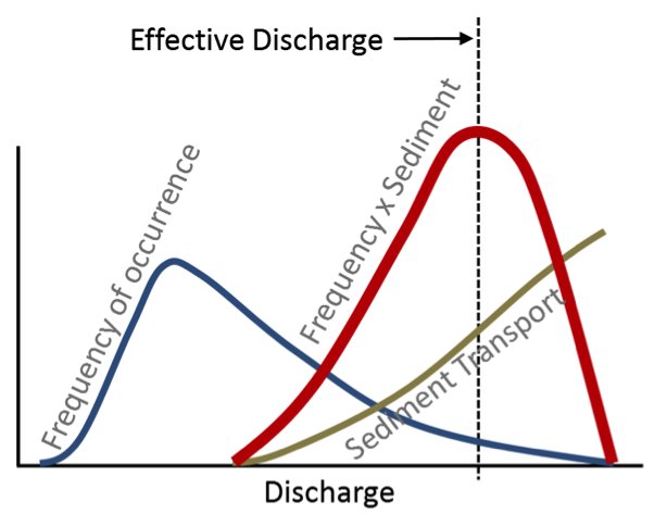
River channels are self-formed. Typically they are only partially filled, the water level is well below the tops of the banks. Sometimes, they are overfilled and water spills out onto the floodplain. These simple observations lead to the fundamental question, ‘what sets the size of a river channel?’ igure 31 conceptually illustrates the rationale supporting the empirical finding that an ‘effective discharge’, which occurs frequently enough and has sufficient power to do work, ultimately dictates the size of the channel. Specifically, the brown curve illustrates that the frequency distribution of discharge in a river is typically right (positively) skewed, meaning that relatively low discharges are quite common and increasingly higher discharges occur with diminishing frequency. There is some discharge below which sediment does not move on the river bed because there is insufficient power to move the sand or gravel, as indicated by the light orange line starting at some moderate discharge and increasing in a non-linear manner at progressively higher discharge. Multiplying the brown and light orange lines together yields the darker orange line, which has a peak at some relatively high discharge value. This ‘effective discharge’ tends to occur when the river is approximately full up to its naturally formed banks. Even very large floods, which greatly exceed the capacity of the channel, do not necessarily add a proportionate amount of power to the channel because much of the additional water (and therefore the energy to transport sediment) is dissipated on the adjacent floodplain.
As changes in climate alter precipitation patterns or as land and water management modulates the proportion of precipitation that becomes streamflow, the frequency curve in Figure 31 may change and thus change the effective discharge as well as the geometry of the channel. In this way, rivers are dynamic features in the landscape, growing bigger when more water is flowing through the landscape and smaller during extended drier periods.