Module 4: Flood and Drought
Module 4: Flood and Drought
In this module, we will discuss the causes, implications and ways to characterize and predict what are often referred to as ‘extreme events’ in hydrology: floods and droughts. Such events play important roles in natural ecosystems and are a major concern for society, with significant impacts on the economy, ecosystem health and services, as well as human health. To gain a broader perspective, we will discuss floods and droughts within the more general topic of hydrologic variability. We will look beyond simple metrics like average annual rainfall to instead think about the full distribution of ‘events’ that characterize the hydrology of an area. The goals of this module are to expose you to the basic concepts of floods and droughts, develop an understanding of how we characterize ‘normal’ and ‘extreme’ hydrologic events, and gain some perspective on the consequences of floods and droughts for society and ecosystems. As part of this, you will become familiar with terms such as stationary versus non-stationary conditions, return period (a.k.a., recurrence interval), exceedance probability, and probability density function.
Goals and Objectives
Goals and Objectives
Goals
- Describe the two-way relationship between water resources and human society
- Explain the distribution and dynamics of water at the surface and in the subsurface of the Earth
- Synthesize data and information from multiple reliable sources
- Communicate scientific information in terms that can be understood by the general public
- Interpret graphical representations of scientific data
Learning Objectives
In completing this module, you will:
- Distinguish between a forecast and a prediction and provide examples of each
- Interpret flood frequency patterns from a histogram
- Interpret flood risk at various locations using flood risk maps
- Explain the hazards of living in a floodplain and the utility of floodways
- Assess flood risk and flood history in your own hometown
- Articulate the concept of a 2, 10 and 100-year flood
Making Sense of Hydrologic Variability
Making Sense of Hydrologic Variability
Video: Advanced Hydrologic Prediction Service (1:37)
This short video introduces the NWS Advanced Hydrologic Prediction Service that provides alerts for droughts and floods in the United States.
Precipitation and streamflow are both incredibly variable aspects of the environment, often changing dramatically over short time scales and small spatial scales. If you look up the precipitation record for a location of interest (data freely available from the National Weather Service, Natural Resource Conservation Service, and many other outlets), you would see that events seem to happen ‘randomly’, often without an obvious pattern in the frequency, magnitude or duration. Take, for example, the precipitation record for Kingston, New York from October 1, 2010, through September 30, 2013 (Figure 1). There is an immense amount of variability from day to day. So what can we really say about precipitation from these data? July and August of 2011 appear to be a very wet time period, with many events clustered and one event reaching over 12 cm (nearly 5 inches)! Do you think that caused a flood? Precipitation was very sparse from mid-December 2011 to mid-February 2012. Do you think that was a drought?
It is essentially impossible to answer the questions posed above about July 2011 being a flood or winter 2011-2012 being a drought from the precipitation data alone because precipitation is not the only factor that causes floods and droughts. Processes of water use and transport occurring in a landscape also matter. For example, an increased impervious surface associated with urbanization is known to dramatically increase runoff, resulting in much higher peak discharge (bigger floods) for any given amount of rainfall. In contrast, a large rain event occurring on dry soil will have a relatively small effect on streamflow compared with the same rainfall event occurring on very wet or saturated soils, because more of the rain would be absorbed by the dry soil. Landscape processes also influence droughts. While a prolonged lack of precipitation can initiate a drought, the severity of the drought is strongly influenced by the water demand, by vegetation and/or humans, throughout the landscape. Landscape processes can amplify or dampen precipitation variability. This greatly complicates the job of forecasting floods and droughts. Hydrologists must account for numerous factors that vary in time and/or space.
Though it is difficult, hydrologists can make remarkably accurate and timely predictions of floods and droughts. For example, the National Weather Service (NWS) uses large amounts of real-time data from precipitation gauges, radar systems, river discharge gages, and satellite imagery. The NWS maintains a network of 13 river forecast centers and 50 hydrologic service areas that provide real-time flood warnings throughout the US, which can greatly reduce loss of life and property damages.

Forecasting and Predictions
Forecasting and Predictions
Meteorologists have made excellent progress in the past few decades to improve our abilities to forecast when rain events might occur over the next week or so, which facilitates the short-term forecasting of floods and droughts discussed in the paragraph above. However, complex atmospheric dynamics prevent forecasts beyond more than a few weeks in advance. Nevertheless, we must have some basis for making decisions about development, infrastructure and agriculture (e.g., How big should we build a culvert under a road? What size retention basin is needed next to a new housing development? Which agricultural fields will require artificial drainage and which will require irrigation?).
For these longer-term predictions we can use statistics to determine how likely it is that a given location will experience, for example, more than 10 cm of rain in a day, or less than 5 cm of rain during a given month. Many million- and billion-dollar decisions about development and infrastructure are based on such predictions.
To make these predictions, hydrologists synthesize historical data and use a statistics-based approach to determine the likelihood that a given event might occur. While Figure 1 highlights the ‘messiness’ of precipitation events over time, reorganization of the data provides useful information. Figure 2 shows a histogram of the precipitation data presented in Figure 1. A histogram is a plot showing the number of events that fall within chosen data groups or “bins” (shown on the x axis). From these data you can quickly determine that Kingston, NY experiences no rain about 2 out of every 3 days (731 out of the total 1096 days in this record). Only 10 days in the record had rainfall that exceeded 6 cm, so from these data alone you would expect such large rainfall events to happen 10 days out of 1096, or about 1% of the time. On 210 days during this time period the amount of rainfall was between the minimum measurable (typically 0.025 cm or 0.01 inch) and 1 cm (0.4 inches).
Hydrologists tend to use the term ‘forecast’ when referring to a future projection for which we have a lot of information (and therefore relatively high certainty of when an event might occur and what magnitude it might be). In contrast, hydrologists use the term ‘prediction’ for future projections for which less information is available, and therefore uncertainty is greater.

Learning Checkpoint
The National Weather Service maintains a Precipitation Frequency Data Server (PFDS) website [1] that allows you to look up the frequency of precipitation events of different duration and magnitude for most locations in the US. The PFDS website will open in a new window. Peruse the website and answer the following questions:
Zoom in on Logan, Utah and place the red crosshair directly over Logan. Below the map a table will appear showing the amount of precipitation associated with a range of time periods (durations shown in left column, ranging from 5 minutes to 60 days) and the average frequency with which such an event might happen (the recurrence interval, listed in years).
1. What is the amount of precipitation that you would expect to get in Logan, Utah on an annual basis, within a 24 hour time period?
(a) 0.1 inches
(b) 0.7 inches
(c) 1.2 inches
(d) 2.4 inches
2. What is the amount of precipitation that you would expect to get in Logan, Utah on an annual basis, within a 60 minute time period with a frequency of once every 10 years?
(a) 0.1 inches
(b) 0.7 inches
(c) 1.2 inches
(d) 2.4 inches
(a) 0.1 inches
(b) 1.3 inches
(c) 2.1 inches
(d) 3.3 inches
4. What is the amount of precipitation that you would expect to get in Chickamauga on an annual basis, within a 60 minute time period with a frequency of once every 10 years?
(a) 0.1 inches
(b) 1.3 inches
(c) 2.1 inches
(d) 3.3 inches
Predicting Frequency and Magnitude
Predicting Frequency and Magnitude
We can do similar calculations to estimate the frequency and magnitude of floods. For example, Figure 3 shows the annual maximum series of flows for the Lehigh River at Bethlehem, PA from 1910 to 2013. The annual maximum series is simply the highest flow value recorded for each year (typically for the water year, October 1 – September 30 as discussed in module 3). The largest flow on record (92,000 cfs) occurred in 1942 (on May 23, to be exact). Note that these are daily flow values which average flow over the course of the entire day, so the actual peak that occurred on May 23 was probably slightly higher. Interestingly, the year that had the smallest peak discharge on record was April 6, 1941 (only 8210 cfs, less than 10% of the whopper flood that came through the following year). But note that we are still talking about the highest flow for that particular year, which is still considerably higher than the average annual flow which is about 1,300 cfs. How can we use this information to predict what might happen in the future to support decisions about development, flood risk, or factors that may influence biota in the river or floodplain (e.g., factors limiting the return of certain fish)?
Similar to the precipitation example above, it helps to reorganize the data. The histogram shown in Figure 4 illustrates the frequency of events in 19 different “bins”. For example, the Lehigh River at Bethlehem, PA has never experienced an annual peak flow less than 5,000 cfs, so there is no orange bar in that bin. But it has experienced 4 peak flows that fall between 5,000 and 10,000 cfs. It has experienced a total of 55 peak flows that fall within the range of 10,000 to 25,000 cfs. These are the most common peak flows for the Lehigh River. And you can see the two outliers at the high end (92,000 cfs in 1942 and 91,300 cfs in 1955).
Typically, hydrologists will approximate the distribution of events that you see in Figure 4 as a probability density function, represented by the smooth, dashed-grey curve superimposed on the plot. This allows them to integrate under the curve above a value of interest to determine the probability that a flood of that magnitude (or larger) will occur. For example, integrating to find the area under the grey dashed curve above 60,000 cfs in Figure 4 would tell you the probability in any given year (in the future) that a flood of that magnitude (or larger) will occur. From that information, you can build your bridge to the appropriate size, or set your flood insurance rates accordingly, etc. Calculating probabilities associated with floods of a given magnitude is discussed in greater detail in the exercise associated with this module.
The same general principles apply to studying droughts. However, as we discuss below, droughts are more difficult to define and quantify because they build up over time and vary immensely over any given area. Nevertheless, similar plots of drought frequency, severity and duration can be developed for droughts, similar to Figure 4, to make sense of all the messy variability we observe in water deficiencies. With this brief introduction hopefully you can appreciate the great challenges in predicting the occurrence and severity of floods and droughts, and you can begin to see the implications for socio-economic systems and ecosystems.


Normal Versus Extreme Hydrologic Events
Normal Versus Extreme Hydrologic Events
The immense variability observed in precipitation and streamflow leads one to wonder what constitutes an ‘extreme’ event. For example, most rivers tend to flood (i.e., water completely fills the channel and spills out onto adjacent floodplain) every one to five years. River discharge during such events is often on the order of 10 times the mean annual flow and often 100 to 1000 times greater than the lowest flows. In that context, perhaps they are extreme. However, considering them within the context of all the floods that occur over a century, we refer to floods that occur every one to five years as ‘common floods’ (e.g., all the events below ~ 25,000 cfs for the Lehigh River in Figure 4 shown earlier). So, labeling an event as ‘extreme’ requires some timescale context. Similarly, what we consider ‘extreme’ varies from place to place. For example, a rainfall event that delivers 5 cm of precipitation is quite rare in Utah but is nearly a daily occurrence in parts of Hawaii.
While there is no formal, universal definition for what hydrologists consider to be ‘extreme’ events, there are numerous ways we can assess precipitation and streamflow events within the appropriate context (timescale and location) to determine how they compare with ‘normal’ conditions.
Notice that the distribution of flood events in Figure 4 (on a previous page) has a strong right (also called positive) skew, meaning a long tail to the right of the graph. This positive skew is common in flood frequency data. It is tempting to label the two events that exceed 90,000 cfs as extreme events, but for many rivers there is no clear cut-off. Instead, hydrologists commonly determine the rarity of an event by calculating the frequency with which the event has occurred in the past. They use that frequency as an estimate of the probability that it will occur in the future, as discussed in the example of the Lehigh River. This is useful way to make predictions, but note that climate change prevents us from using the past to predict the future. If the entire event distribution shifts due to climate change, the event probabilities also change. We will address this issue towards the end of the module.
In any case, terms like ‘extreme’ may be useful for news headlines and catchy titles for scientific presentations, but nature doesn’t easily fit into boxes like ‘extreme’ and ‘normal’. Instead, hydrologists tend to use more well-defined terminology to characterize hydrologic events according to their frequency, duration, and magnitude as well as the spatial extent. Events that occur infrequently (i.e., events of low probability) are the ones to watch out for!
Floods
Floods
Video: Floods 101 | National Geographic (3:27)
This brief video from National Geographic describes the basics of flooding.
Floods are rare events in which a body of water temporarily covers land that is normally dry. Following from module 3, we will mostly restrict our discussion to floods in rivers, but it is important to note that floods also occur around lakes, wetlands, and the sea coast. Indeed, coastal storm surge is among the most dangerous natural disasters expected to result from global warming and sea level rise. River floods occur naturally and in many cases are beneficial for ecosystem functioning because they allow the river to exchange water, sediment, and nutrients with the floodplain and cause scour and deposition that provides habitat for a wide range of aquatic and riparian organisms. However, floods often threaten human infrastructure and livelihoods and can cause severe economic damages.
River floods are typically caused by excessive rainfall and/or sudden melting of snow and ice. Most rivers overflow their banks with small floods about once every two years. Such are the floods that tend to determine the width and depth of a river channel, as discussed in module 3. Moderate floods might occur once every five to ten years and very large floods might only occur once in fifty or a hundred years. The average time period over which a flood of a particular magnitude occurs is called that flood’s recurrence interval, or return period. For example, the very large flood that only occurs, on average, once in a hundred years has a 100-year recurrence interval and is therefore called the 100-year flood. Relating this notion of recurrence interval to the section on probability, above, the recurrence interval is simply the reciprocal of the probability associated with an event (i.e., T = 1/p, where T is the recurrence interval and p is the probability that such an event will occur (or be exceeded), as computed by integrating under the dashed line shown in Figure 4, above the event magnitude of interest). The probability of a 100-year event occurring in any given year is 0.01, or 1%.
We should pay careful attention to our terms here. Note that we are talking about the average time period expected between events. Just because a 100-year event happened last year, there is nothing that says it cannot happen again this year. In fact, the probability of two 100 year floods occurring in back-to-back years is 0.01 times 0.01, or 0.0001. This suggests that, if everything stays the same, the 100-year event should happen in back-to-back years about once every 10,000 years. Of course, over 10,000 year time periods most things don’t stay the same. We’ll discuss this issue, termed non-stationarity, towards the end of the module.
Flash floods are typically caused by heavy rains falling on soils that are already wet or frozen (and therefore have limited capacity to absorb more water), or on land that is covered by snow (in which case the frozen soil has limited capacity to absorb water and the situation is compounded by the fact that melting snow adds to the runoff). Flash floods allow very little time for people downstream to be warned and are therefore especially dangerous. For example, in April 2024, Rio Grand du Sol, Brazil experienced over 30 inches of rainfall over two weeks leading to 150 deaths, 500,000 people displaced from their homes, and over $10 billion in damages.

Expansion of urban areas can increase the frequency, magnitude, and flashiness of floods. Impervious surfaces (roads, parking lots, and buildings) route precipitation directly to stream channels and prevent draining of water slowly through soils to groundwater (Figure 5). The term flashiness refers to the rate at which the water levels rise and fall with faster rising and falling water levels considered flashier.

Hydrologic Versus Hydro-Geomorphic Perspectives
Hydrologic Versus Hydro-Geomorphic Perspectives
Scientists tend to think about floods in two different (but related) ways, one being strictly hydrologic and the other requiring an evaluation of the floodplain topography and how different flow regimes might impact the channel and surrounding areas. In module 3, we explored how hydrologic analyses (analyzing the patterns such as the frequency, duration, and magnitude of flood events) could be used to characterize the river flow regime (e.g., how often does the river exceed 800,000 cfs?). However, a hydrologic analysis does not provide information about the extent or duration of flooding across the landscape (e.g., which parts of the natural floodplain or streets will be flooded?). To predict how much of the floodplain might be inundated by a given flow, we need to consider the channel and floodplain topography (a hydro-geomorphic analysis). For example, a river system with low channel banks and a broad, flat floodplain will experience more frequent flooding of greater extent than a river system with tall banks and a narrow floodplain, given the same flow regime.
Because the size of a river channel can change over time, the relationship between the hydrologic flood frequency and hydro-geomorphic mapping of the area inundated may also change, as discussed in the later module section on hydrologic non-stationarity. For example, the Minnesota River (a major tributary of the Mississippi River) has widened by nearly 50% in the past 3-4 decades. Therefore a flood that may have inundated a significant amount of floodplain 50 years ago may now be entirely conveyed within the channel itself. Thinking back to the example of the Lehigh River in Figures 4 and 5 it is very likely that the 1941 flood (the lowest on record) did not fill the channel and inundate the floodplain. 1943 and 1944 had moderately high peak flows, but may also not have gotten out of the channel because the massive 1942 flood would have widened and deepened the channel. Over the following years, the channel would likely have narrowed again, in response to relatively smaller floods. Flood frequency analysis discussed below and in the exercise associated with this module, is strictly a hydrologic analysis. A hydro-geomorphic analysis is needed to estimate the risk of flood damage. Both types of analyses may be important for engineering plans and ecological studies. High-resolution topography data (elevation data with a vertical precision of about 15 cm and horizontal resolution of about 1 m, also known as ‘lidar’ for Light Detection and Ranging) is revolutionizing the way we make flood inundation predictions. Lidar data contains very detailed information about the ground surface, as well as vegetation on the floodplain, which exerts a strong influence on the velocity and depth of the water. Many states are revising their flood risk maps using this new high-resolution data.
Societal and Economic Implications of Floods
Societal and Economic Implications of Floods
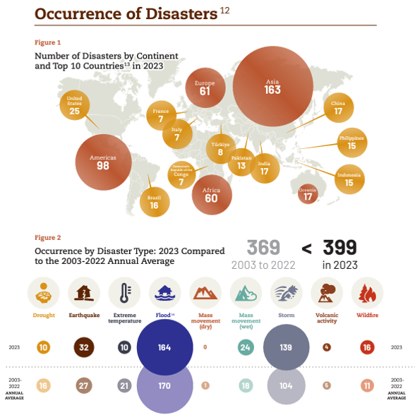
Floods are consistently ranked among the most costly natural disasters around the world, with many billions of dollars in damages reported annually. For example, the Centre for Research on the Epidemiology of Disasters International Disaster Database [3] (EM-DAT) reports that floods accounted for four of the ten most deadly natural disasters in 2013, with confirmed global fatalities exceeding 5000 people (EM-DAT, (2023)). The same 2023 report documents $20.4 billion in damages directly related to river floods.
| Event | Country | Number of Deaths |
|---|---|---|
| Earthquake | Turkey | 50,783 |
| Storm Daniel | Libya | 12,352 |
| Earthquake | Syrian Arab Rep | 5,900 |
| Flood | Congo | 2,970 |
| Earthquake | Morocco | 2,948 |
| Earthquake | Afghanistan | 2,445 |
| Flood | India | 1,529 |
| Tropical Storm | Malawi | 1209 |
| Flood | Nigeria | 275 |
| Flood | Yemen | 248 |
| Total | 80,681 |
During late spring and summer of 1993 heavy rains all throughout the Midwestern US resulted in flooding along the upper Mississippi and Missouri river systems. The floods were the most costly in US history, causing about $15 billion in damages and forcing about 75,000 people from their homes. Heavy rains from Tropical Storm Irene in August 2011 caused approximately $10 billion in damages throughout the Caribbean and eastern United States (including flooding Kingston, NY during the wet period indicated in Figure 1). Notably, the numbers of fatalities associated with these extreme events were relatively low (~50 deaths each) due to remarkably accurate flood forecasting, highly effective emergency response systems and regulations that limit development in flood-prone areas.

Rivers that cannot transport their sediment load (sand and gravel) are particularly susceptible to flooding because sediment settles out in the river bed, causing the river channel to become shallower relative to its banks, thus increasing the chances of flooding. The Yellow River in China is one example of such a river. While the Yellow River has played a pivotal role in the Chinese economy for thousands of years, sedimentation has repeatedly caused the river channel bed and banks to actually build up higher than the surrounding floodplain. This is an especially dangerous situation that can cause the river to catastrophically flood, breach its banks, abandon its channel altogether, and ultimately form a new channel elsewhere within the floodplain, a process known as an avulsion. The Yellow River has caused many devastating floods, including a flood in 1332-1333 that killed an estimated 7 million people. Another Yellow River flood in September of 1887 inundated an estimated 130,000 km2 (50,000 square miles, an area approximately the size of Alabama!) and killed an estimated million people. Yet another flood in 1931 is estimated to have killed 1-4 million. Such catastrophic disasters have earned the Yellow River its nickname, ‘China’s Sorrow.’
Humans have made extraordinary efforts to reduce flood damages. In some cases, these efforts involve limiting development in flood-prone areas. In other cases, these efforts involve building structures meant to control the floodwaters. Flood control structures include dams and retention basins that store water and/or building levees, dikes, and floodwalls that attempt to keep floodwaters confined. Some of the most extensive flood control systems in the world include the floodway diversions on the Red River, which runs between Minnesota and the Dakotas and crosses the US-Canada border into Manitoba.
While we typically think of floods as dangerous and costly natural hazards, they can also provide benefits to society. For example, floods naturally deliver fresh, nutrient-rich sediments to their floodplains, which have historically benefited farmers in many places throughout the world. Yearly floods of the Nile River allowed the early Egyptian people to grow crops, which helped them thrive as a civilization for thousands of years. However, the severity of the floods was unpredictable and floods that were too large caused significant damage. Therefore, in the mid-1900s the Egyptians constructed a flood-control dam on the Nile River. The dam eliminated both the risks and benefits of annual flooding and therefore agricultural practices have had to adapt by using irrigation and petroleum-based fertilizers to replace the water and nutrients that are no longer delivered to the floodplain by the river.
Flood control is not always feasible, given the unpredictable nature of these events as well as geographic or economic constraints. Nor is flood control necessarily desirable in many situations, given the potential environmental benefits for the river and floodplain discussed at the beginning of this section and discussed in greater detail towards the end of this section. In such cases, efforts can be made to reduce economic losses from floods. For example, in many places regulations limit the construction of permanent buildings on floodplains. Emergency response programs, such as the National Weather Service and Federal Emergency Management Agency (FEMA) help flood victims by improving methods to warn and evacuate people from flood-prone areas and to provide relief aid. In an alternative approach, communities in Tonle Sap, Cambodia have constructed their houses on floats and stilts to deal with the annual flooding of 8-9 m (26-30 ft) from the Mekong River.

In many places, flood insurance can be purchased to help cover costs associated with residential and commercial flood damages. However, the private insurance industry is somewhat limited because the number of potential claimants far exceeds the number of people who wish to ensure their property against flooding. As a result, the US Congress created the National Flood Insurance Program in 1968. The program is an effort to provide flood insurance to protect homeowners, renters, and business owners as well as an effort to encourage communities to adopt flood risk management policies established by FEMA.
Droughts
Droughts
Video: California's Extreme Drought, Explained (3:33)
This short video from the New York Times describes the economic and environmental impacts of the severe drought that occurred in California in 2014.
The Wall Street Journal reported that California saw record breaking rains in 2023 and 2024 after a decade of severe drought. In just 2014, 2015, and 2022, California had nearly $7 billion in lost revenue and 40,000 lost jobs in the agriculture sector due to severe drought.
How do you know when you’re in a drought?
Identifying an area as ‘in drought’ is different from identifying it as ‘arid’. While the two may seem related, the subtle difference is important. Aridity is defined as the “degree to which a climate lacks effective, life-promoting moisture” (Glossary of Meteorology, American Meteorological Society). Drought, on the other hand, is ‘a prolonged period of abnormally dry conditions.’ Thus, aridity is a quasi-permanent condition (persistent over human timescales), while drought is a temporary condition (which may persist for weeks, years, or in some cases, decades). The Sahara Desert is an arid environment. The Hoh rainforest in western Washington State is a very humid place that occasionally experiences drought.


Droughts tend to be somewhat elusive phenomena, with severity gradually increasing over many days, weeks, months, or even years. The spatial extent of drought is also quite difficult to delineate, due to the spatial variability in precipitation. Therefore, they are much harder to define, monitor, and identify (relative to floods) within the ‘noisy’ background of natural wet and dry cycles. Yet the impacts of drought can be significant on many facets of the economy and environment. All types of drought originate from a deficiency of precipitation from an unusual weather pattern. If the weather pattern persists for a few to several weeks, it is said to be a short-term drought. However, if precipitation remains well below average for several months to years, the drought is considered to be a long-term drought.


Related to the difficulty in defining drought, economic damages related to drought are also difficult to define. But only considering economic damages that can be directly related to drought, it is clear that they too can be costly natural disasters. In 2023, EM-DAT claims 247 deaths worldwide that were directly attributed to drought (1157 is global annual average from 2003-2022), but a total of nearly \$22 million people were significantly affected by drought in 2023 (average is over \$57 million per year from 2003-2022). Damages related directly to drought in 2023 were estimated in excess of \$22 billion (average of nearly \$9 billion per year from 2003-2022). However, these numbers do not include related effects of wildfire and indirect effects of decreased food production, water quality, etc.
| Phenomenona and direction of trend | Likelihood that trend occurred in late 20th century (typically post 1960) | Likelihood of a human contribution to observed trendb | Likelihood of future trends based on projections for 21st century using SRES scenarios |
|---|---|---|---|
| Warmer and fewer cold days and nights over most land areas | Very likelyc | Likelyd | Virtually certaind |
| Warmer and more frequent hot days and nights over most land areas | Very likelye | Likely (nights)d | Virtually certaind |
| Warm spells/heat waves. Frequency increases over most land areas | Likely | More likely than notf | Very likely |
| Heavy precipitation events. Frequency (or portion of total rainfall from heavy falls) increases over most areas | Likely | More likely then notf | Very likely |
| Area affected by drought increases | Likely in many regions since 1970s | More likely than not | Likely |
| Intense tropical cyclone activity increases | Likely in some regions since 1970 | More likely than notf | Likely |
| Increased incidence of extreme high sea level (excludes tsunamisg | Likely | More likely than notf,h | Likelyi |
Table notes:
a See table 3.7 for further details regarding definitions.
b See table TS.4, Box TS.5 and table 9.4.
c Decreased frequency of cold days and nights (coldest 10%).
d Warming of the most extreme days and nights of each year.
e Increased frequency of hot days and nights (hottest 10%).
f Magnitude of anthropogenic contributions not assessed. Attribution for these phenomena based on expert judgment rather than formal attribution studies.
g Extreme high sea level depends on average sea level and on regional weather systems. It is defined here as the highest 1% of hourly values of observed sea level at a station for a given reference period.
h Changes in observed extreme high sea level closely follow the changes in average sea level. {5.5} It is very likely that anthropogenic activity contributed to a rise in average sea level. {9.5}
i In all scenarios, the projected global average sea level at 2100 is higher than in the reference period. {10.6} The effect of changes in regional weather systems on sea level extremes has not been assessed.
There are four different kinds of drought.
- Meteorological drought refers to a deficit in precipitation that is unusually extreme and prolonged. By definition, meteorological drought must be identified relative to the typical precipitation regime of an area and could be defined as some point out on the long-tail of the distribution of, for example, a plot (histogram or probability density function) similar to Figure 4 [5], except with the x-axis indicating the number of consecutive dry days.
- Agricultural drought refers to a deficit in soil moisture that affects plant growth and productivity. While this term is most often used to refer to effects on agricultural crops, all plants can be affected by soil moisture drought. Paleoclimatologists (scientists who study past climate) examine the thickness of tree rings in woody plants to estimate the timing, duration, and severity of past droughts because water-stressed trees form relatively narrow rings in drought conditions.
- Hydrological drought refers to conditions in which stream discharge and/or lake, wetland and water-table elevations decline to unusually low levels.
- Socio-economic or operational drought refers to conditions when water supply is significantly below demand such that water/reservoir management must be altered. Typically, when meteorological drought occurs, the effects cascade sequentially to the other three types of drought. Likewise, when the meteorological drought ends, the effects cascade in the same sequence, first restoring soil moisture, then restoring other hydrological ‘stocks’ within the system, and hopefully restoring the balance between water supply and demand at key water management infrastructure (i.e., reservoirs).
Activate Your Learning
Go to the US Drought Monitor webpage [6] and answer the following questions:
1. Is the place where you live currently in a drought?
2. Looking back through historical maps, when was the last time your home town was in a drought?
Measuring the Severity of Drought
Measuring the Severity of Drought
Many different indices have been developed over the past several decades to indicate the occurrence and severity of drought. The simplest index relates precipitation amounts during a specific period of time to the historical average during that same time period. For example, precipitation for the month of June 2014 was 15% below the historical average for Wenatchee, Washington. While this statement conveys some useful information, it is not possible to determine whether or not that 15% deficit qualifies for any of the definitions of drought. The number of days with no precipitation is another simple index, but again must be considered in the context of historical data or water demand, and there is no standard definition for what number of days without precipitation would necessarily qualify under any of the four types of drought. Also, if an area receives a very small amount of precipitation (< 0.1 cm) during an otherwise unusually dry time period, a strict interpretation of this index would ‘reset the clock’, but in reality, the severity of the water deficit remains essentially unchanged. Complex phenomena, such as drought, require somewhat complex metrics to be measured in a meaningful way.
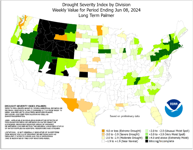
The Standardized Precipitation Index (SPI) is a slightly more complex measure of precipitation deficit that compares measured precipitation to the median historical precipitation over multiple timescales, ranging from one month to 24 months. As dry or wet conditions become more severe, SPI becomes more negative or positive, respectively. Several different indices of varying complexity have been developed to assess drought based on both water supply and demand using multiple environmental criteria. The most common index used to define and monitor drought is the Palmer Drought Severity Index (PDSI), which attempts to measure the duration and intensity of long-term, spatially extensive drought, based on precipitation, temperature, and available water content data. PDSI ranges from values exceeding 4.0, which are considered extremely wet, to values below -4.0, which are considered extreme drought (see Figure 12). Weekly maps of PDSI for the entire US (current and historical) can be viewed on the web page maintained by the National Weather Service Climate Prediction Center [7].
Related indices are the Palmer Z Index, which attempts to measure short-term drought on a monthly timescale, the Palmer Crop Moisture Index, which attempts to measure short-term drought and quantify impacts on agricultural productivity, the Palmer Hydrological Drought Index, which attempts to estimate the long-term effects of drought on reservoir levels and groundwater levels. An immense compilation of current and historical drought information for the entire US is freely available on the US Drought Monitor web page [6], maintained by the University of Nebraska National Drought Mitigation Center.
Increasingly, government and industry groups are using ‘cloud seeding’ techniques to induce precipitation and reduce the severity of a drought. One of the potentially limiting steps in the formation of precipitation is the presence of tiny particles (nuclei) on which water can condense and coalesce to form raindrops or ice crystals large enough to begin falling through the air. Cloud seeding is the practice of injecting nucleating agents, such as silver iodide (AgI), into clouds in an attempt to form precipitation. The effectiveness of these approaches is questionable, but under the right conditions, cloud seeding may increase the probability of rain and therefore it is practiced in some semi-arid regions, including the western US. However, questions remain regarding environmental and human health impacts as well as concerns regarding ‘stealing’ atmospheric moisture from would-be recipients downwind.
Learning Checkpoint
1. What was the Palmer Drought Severity Index for the week ending on June 8, 2024, for the following locations (see Figure 12 above):
St. Louis, Missouri
San Antonio, Texas
Boston, Massachusetts
2. Which of these three locations were likely experiencing socio-economic drought during this time, forcing them to actually change water use/management practices, at least temporarily?
San Antonio, Texas
Boston, Massachusetts
Miami, Florida
Floods and Droughts Impact Ecosystems
Floods and Droughts Impact Ecosystems
How do floods and droughts impact ecosystems?
Variation in river flow (i.e., the river flow regime – see Module 3) exerts a strong influence on river and riparian ecosystem function. In particular, floods and droughts control the creation and maintenance of river and floodplain habitats and the sustainability of the high biodiversity observed along river systems. The temporal pattern of floods interacts with channel and floodplain topography to create a highly heterogeneous landscape of depressions, oxbows, gravel bars, and terraces (Figure 13). The hydro-geomorphic diversity means that the inundation frequency varies strongly over short distances on river floodplains, and creates habitats for a diverse suite of organisms adapted to a wide range of flooding frequencies.

Both riparian and aquatic organisms have adapted to take advantage of flood-drought cycles in river ecosystems. For example, many fish species time spawning runs to coincide with predictable floods, because this allows large adult fish to access small streams that provide optimal habitat for egg development and growth and survival of young fish. In the Amazon River, many fish species can almost be considered forest-dwelling fish, because they feed directly on leaves, fruits, seeds, and insects that fall into the river when it floods surrounding forests during the annual rainy season. Trees of these seasonally flooded forests have in turn developed fruits and seeds that mature during the flooding season and that can survive fish digestive systems in order to take advantage of the seed dispersal ability of mobile fish species. In the western U.S., cottonwood trees time the release of seeds to coincide with the recession of flood peaks in order to access fresh sediment deposits with elevated water tables that provide ideal habitats for germination.
It may be less obvious that droughts could be beneficial for aquatic and riparian biota, but when coupled with periodic flooding, droughts play an important role in the survival of many river organisms. During droughts, resources such as organic material and nutrients can accumulate on floodplain surfaces, and when a flood does occur there is a pulse of greater resource availability than would occur under regular flooding, and this period of high resource availability can ensure the quick growth and survival of organisms, including young fish. In addition, periodic drying of rivers and floodplain wetlands eliminates competitors and predators for organisms that can quickly colonize areas when water returns. Such areas of refuge from predators are critical for the persistence of many aquatic organisms and would not exist without periods of drought.
The importance of floods and droughts to the integrity of river-floodplain ecosystems is apparent when alterations to the natural flow regime occur. Riverine organisms are often closely adapted to the local magnitude, frequency, duration, and predictability of extreme events, such that alteration of any one component can threaten species persistence. For example, recruitment of cottonwood trees along many dammed rivers in the western U.S. has essentially ceased, because the dams prevent flooding and creation of germination sites during the spring when cottonwood trees release their seeds. Excessive drought is also highly detrimental to river systems. One of the most famous examples of drought impacts is seen in the Colorado River delta in Mexico, which was once a highly productive floodplain forest and swamp, but due to prolonged drought conditions in the river basin and water infrastructure development, is now a dry desert.
Hydrologic Variability Versus the Human Need for Water Resource Reliability
Hydrologic Variability Versus the Human Need for Water Resource Reliability
Floods and droughts are natural phenomena throughout the world and natural systems have adapted to this variability over time. But human demands for water resources are not so adaptable to variable hydrologic patterns. What if you could only turn on the tap during and immediately after rainfall events? Hydroelectric dams also require a constant supply of water to respond to electricity demands on timescales of minutes and hours. Farmers in drier areas require a reliable supply of water to keep crops watered and soils from drying out. In response to societal needs for a reliable and sufficient supply of water, we have developed an extensive infrastructure to even-out variability in natural flow regimes and therefore reduce uncertainty associated with both floods and droughts.
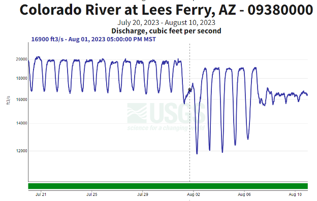
In particular, dams and reservoirs have been constructed around the world to store water during times of flood and provide water during times of drought – as discussed in detail in the next module (Module 5) (Figure 14). Over half of the world’s large river systems (those holding 60% of the world river discharge) are impacted by dams. In fact, the construction of dams and associated filling of reservoirs slows the rotation of the Earth (though only adding ~0.1 microseconds to the length of a day)! However, as we will see in Module 5, the construction of dams and evening out of hydrologic patterns has profound impacts on geomorphic and ecological processes in river systems, and the manipulation of discharge leads to reduced variability in flow regime (e.g., Figures 15 and 16), among many other effects.


Non-Stationary Hydrology
Non-Stationary Hydrology
When ‘normal’ changes: non-stationary hydrology
As we have discussed at length above, floods and droughts can have significant impacts on society and the environment. However, as also discussed above, we can characterize the frequency, duration and magnitude of these rare or extreme events and both human and natural systems have mechanisms to deal with them. For example, we can estimate the magnitude of a 100-year flood and build a bridge sufficiently large to pass the flood with minimal risk of damage to the bridge or changes in water depth (i.e., from water backing up behind the bridge and therefore flooding additional land upstream). Similarly, we can compute the width of a floodplain that would be inundated from that 100-year flood and choose to not build within that flood corridor, or choose to require those who do build within the flood corridor to purchase flood insurance to cover costs of potential damages.
Similarly, as we discussed in module 3, river channels naturally adapt their width and depth to accommodate common floods. Thus, society and the environment naturally develop some amount of resiliency to historical climate extremes. However, all of the prediction methods we have discussed so far in this module rely on the assumption that the future will look statistically similar to the past (i.e., the distribution of events will not change and occurrence of events in the future will be consistent with the probabilities computed from the histograms or probability density functions such as those shown in Figures 3 and 4). This assumption is known as the Stationarity Assumption in hydrology. Specifically, stationarity implies that while there is considerable variability in precipitation and streamflow, that variability is bouncing around a relatively constant average value and has a relatively constant spread, as shown in the hypothetical plot of peak streamflow over time in the left panel of Figure 17. From left to right, the mean (µ) and standard deviation (s, i.e., the spread of the data around the mean) don't change. However, as climate changes, the magnitudes, durations, and frequencies of floods and droughts may occur that are outside the historical range of observations, resulting in a change in the average magnitude of floods (Figure 17, middle panel) or a change in the variability of floods (Figure 17, right panel). In either of these situations, the statistics from the left side of the graph don't provide a good basis for making predictions about the right side of the graph (or predicting what will happen in the future!). Understanding and accounting for such non-stationary patterns in precipitation and streamflow are among the greatest challenges in hydrology today because we need to make accurate future predictions for many decisions about flood and drought risk, infrastructure design (roads, bridges, culverts, ditches, parking lots, detention basins, sewers, etc.!) and water availability. So this is a hot topic in the field and many new techniques are emerging!
Non-stationarity will be common in the future as regional climates systematically change. According to the Intergovernmental Panel on Climate Change, climatic warming will increase the risk of both floods and droughts (Table SPM2 in IPCC, 2007; see also IPCC, 2014 and IPCC 2023). The multitude of factors that combine to ultimately cause floods and droughts are exceptionally difficult to predict over the next few decades. Nevertheless, there is a high level of agreement among the competing IPCC climate simulation models regarding the general trends of several metrics. For example, precipitation intensity increases are expected in most places and especially at mid- and high-latitudes where mean precipitation also increases. Summer droughts are also expected to increase over low and mid-latitude continental interiors. Snowpack is expected to decline overall as more precipitation will fall as rain rather than snow, especially in areas with temperatures near 0°C in fall and spring. Relatedly, snowmelt is projected to occur earlier. The combination of less snowpack and earlier snowmelt increases risk of summer to fall drought in snowmelt dependent regions, such as the western US. Some regions outside the US are highly dependent on meltwater from glaciers for water supply. Accelerated melting due to climatic warming increases the risk of flooding downstream in the near-term. In the long-term, glaciers in many of these areas will shrink and ultimately cease to exist, posing a serious threat to the downstream water supply. This poses a serious risk to the hundreds of millions of people in China and India who depend on glacial meltwater from the Hindu Kush-Himalayas. In closing, there is a good reason to expect floods and droughts to become more severe in the coming decades, increasing the urgency for improved predictions, mitigation efforts, and adaptation strategies.