6.2 Aquifer Processes and Dynamics
6.2 Aquifer Processes and Dynamics
In the first half of the module, we’ve explored the properties of aquifers. But, of course, that is only half of the story! In order for groundwater to flow, there must be a driving force. The same is true for surface water like streams or rivers: in that case, the driving force is gravity. In the case of groundwater, the driving force is a bit more complicated because it includes the combined effects of gravity and pressure.
As we will see, these driving forces are partly determined by the natural system but can be perturbed by pumping or injection in wells. When we pump water from wells, we alter the natural driving forces to move water toward the well. One important issue in aquifers is accounting for the flows in to and out of the aquifer in a groundwater budget. In extreme cases, the amount of water extracted at wells may exceed the amount introduced to the aquifer through recharge. As we’ll discuss, this tenuous condition is known as an overdraft.
Goals and Objectives
Goals and Objectives
Goals
- Describe the two-way relationship between water resources and human society
- Explain the distribution and dynamics of water at the surface and in the subsurface of the Earth
- Thoughtfully evaluate information and policy statements regarding the current and future predicted state of water resources
- Interpret graphical representations of scientific data
Learning Objectives
In completing this lesson, you will:
- Apply the concept of hydraulic head to draw flowlines on maps and cross-sections
- Interpret the current and historical balance between groundwater recharge and water extraction from well hydrographs
- Propose a course of action to address overdraft in an aquifer
Driving Forces for Groundwater Flow
Driving Forces for Groundwater Flow
The driving forces that control groundwater flow are a bit more complicated than those controlling flow in rivers and streams. As you learned in Module 3, surface water flows downhill due to gravity, and the flow direction is defined by the topography. Water flows downhill because gravity is a form of potential energy – and the water, or anything that falls or rolls downward – flows in response to differences in potential energy (from high to low).
In contrast to surface water, groundwater is separated from the atmosphere, and as a result, it can be under considerable pressure. Therefore, the potential energy that drives groundwater movement includes both pressure and gravity. In this section, you will learn about these driving forces, how we define them, and how they translate to the direction and rate of groundwater movement in the subsurface.
Potential Energy and Hydraulic Head
Potential Energy and Hydraulic Head
The flow of both surface water and groundwater is driven by differences in potential energy. In the case of surface water, flow occurs in response to differences in gravitational potential energy caused by elevation differences. In other words, water flows downhill, from high potential energy to low potential energy. In groundwater systems, things are a bit more interesting. Unlike surface water, which is in contact with the atmosphere and therefore rarely under pressure, water in groundwater systems is isolated from the land surface. This means that groundwater can also have potential energy associated with pressure. In extreme cases, water in confined aquifers may be under sufficient pressure to drive flow upward, against gravity. Artesian wells are one manifestation of this.
Fundamentally, groundwater and surface water are similar in that flow is in the “downhill” direction. But what does “downhill” mean in a groundwater system? To define the flow direction, we need to account for the two types of potential energy. Unfortunately, the potential energy of the water cannot be measured directly. However, we can measure a proxy for the potential energy by measuring the hydraulic head, or level to which water rises in a well (Figures 26 and 27). The hydraulic head combines two components: (1) potential energy contained by the water by virtue of its elevation above a reference datum, typically mean sea level; and (2) additional energy contributed by pressure. In a well, the value of hydraulic head represents the potential energy of the water at a particular point in three dimensions – at the depth where the well is open to the aquifer (Figures 26-27). This is analogous to a temperature reading taken at the tip of a thermometer, which provides a proxy for heat energy. Hydraulic head can be written as:
h = z + Ψ,
where z is the elevation energy, and Ψ is the pressure energy.


Click to expand to provide more information
Hydraulic Head and the Direction of Groundwater Flow
Hydraulic Head and the Direction of Groundwater Flow
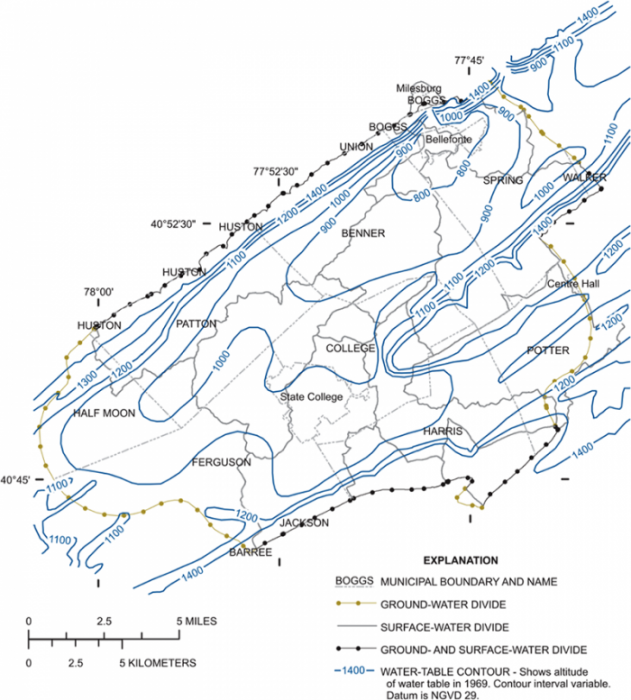
In order to define groundwater flow directions and rates through aquifers, individual measurements of hydraulic head are combined to generate contour maps of water level – or potential energy (Figure 29). These maps define the potentiometric surface, which is much like a topographic contour map but defines the distribution of potential energy in the groundwater system. Each contour, or equipotential, represents a line of equal hydraulic head.
Video: Slag Heap Experiment (3:46 minutes)
To first approximation, groundwater flows down-gradient (from high to low hydraulic head). As is the case with surface water, or a ball rolling down a hill, the water flows in the direction of the steepest gradient, meaning that it flows perpendicular to equipotentials. There are exceptions to this – for example, if the hydraulic conductivity of the aquifer is much higher in one direction than another, or dominated by fractures with particular orientations, then these can redirect groundwater flow askew to the maximum gradient.
The potentiometric map also provides clues about the rate of groundwater flow. If you think back to Darcy material and our in-class activity from last week, you will recall that groundwater flow rate depends on the head gradient (i.e. the hydraulic gradient) and hydraulic conductivity. In a simple one-dimensional Darcy tube experiment, the head gradient is just the difference (h1-h2)/L. In two dimensions, the head gradient is defined by the slope of the potentiometric surface – just as the slope of the land surface is defined on a topographic map. The path that water takes in the aquifer, defined as a continuous line tracing the maximum gradient on a map of the potentiometric surface, is known as a flowline.
Well Hydrographs
Well Hydrographs
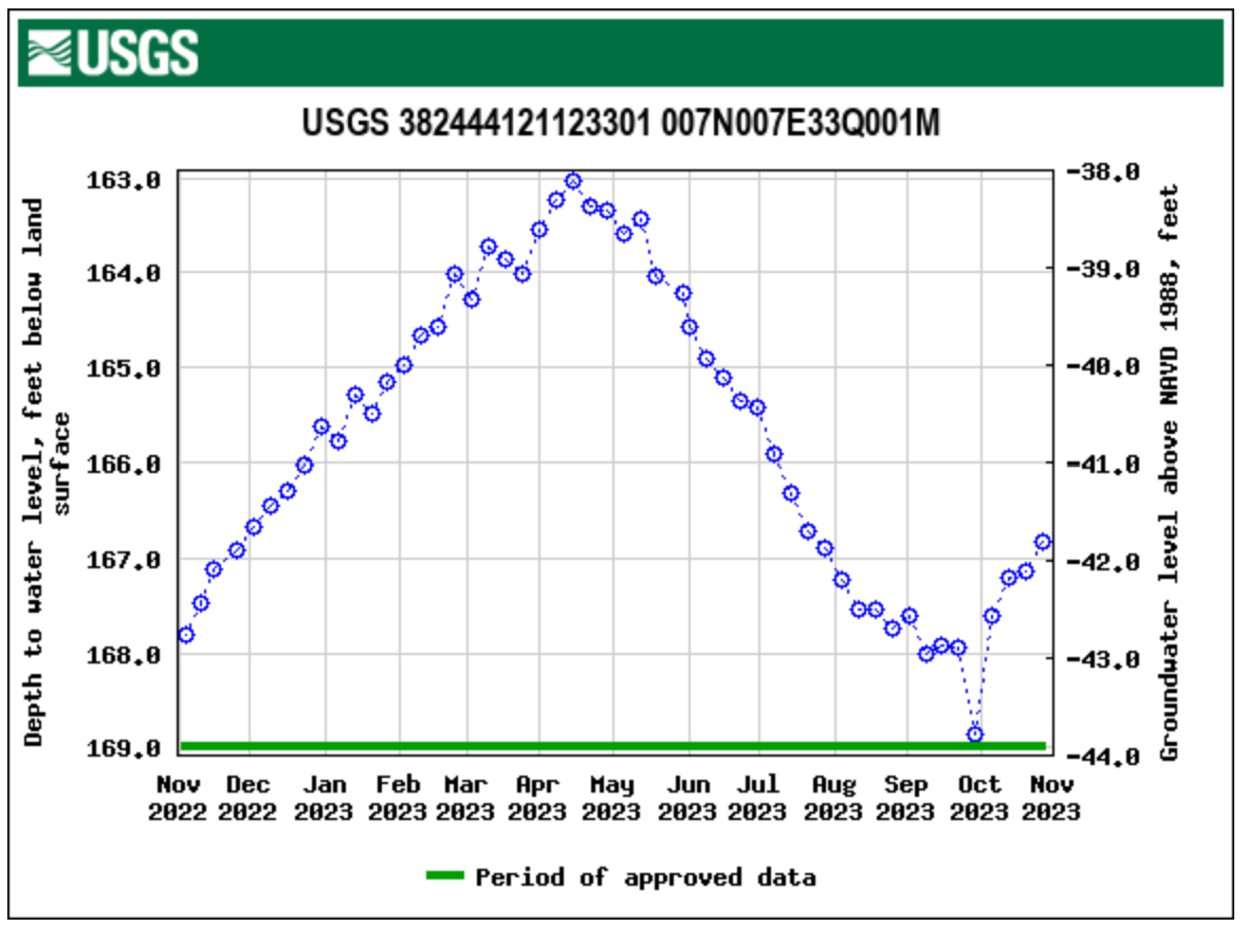
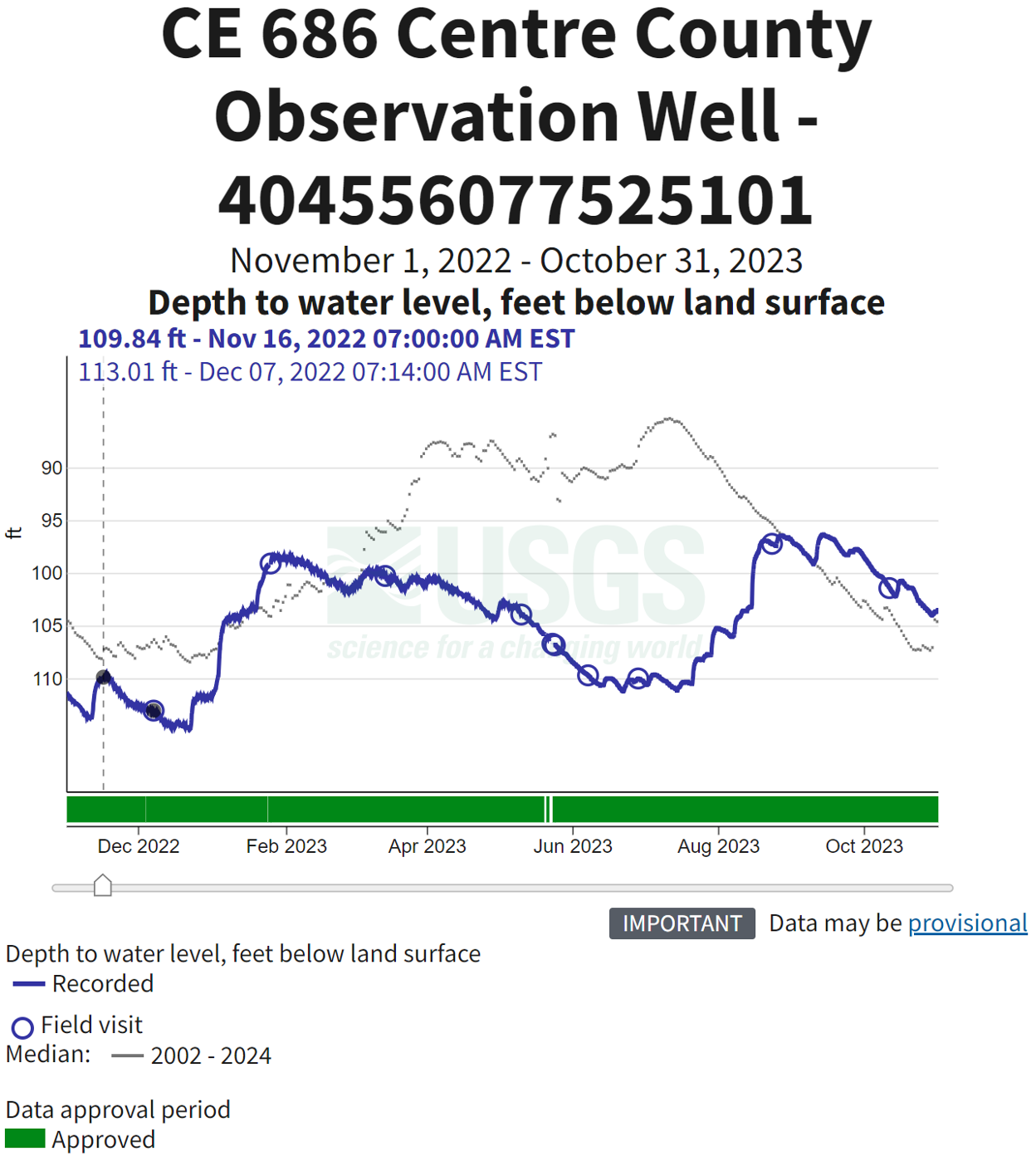
Just as river hydrographs are used to record and visualize variations in flow with time (as discussed in Module 4), a well hydrograph is a time series of hydraulic head recorded in a well. This provides information about the fluctuation of hydraulic head (equivalent to the water table in an unconfined aquifer), which reflects the combined effects of temporal variations in climate, recharge, and pumping (Figures 30-31). The U.S. Geological Survey maintains a database of active monitoring wells [1] in major aquifer systems across the United States. Hydrographs provide information about seasonal patterns that may be associated with pronounced wet and dry seasons typical of some regions (for example, Central CA), as well as long-term trends driven by climate change, decadal-scale climate patterns like el nino, prolonged groundwater extraction, or human-induced modifications to natural recharge. We’ll cover examples of the latter two processes in the next section of the module (Module 6.2: Water budgets).
USGS [3]
Video: Slag Heap Experiment (3:46)
Effects of Pumping Wells
Effects of Pumping Wells
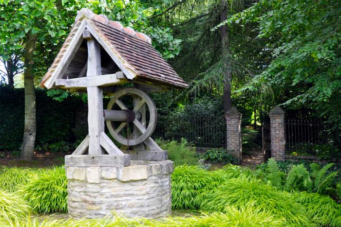
Groundwater is accessed by either pumping from wells drilled into the aquifer (Figure 33), or by developing natural springs where the potentiometric surface intersects the land surface (Big Spring in Bellefonte, PA is one example of a relatively large spring that is used for municipal supply). Although springs are relatively inexpensive to develop, they are not always present, nor are the flow rates always sufficient to support demand. As a result, most groundwater extraction occurs by pumping wells, or in many cases “fields” of wells concentrated in a small area.

Cones of Depression: Pumping at a well, or at a wellfield, pulls water toward the well from all directions – in other words, it induces radial flow (around the radius of the well). In doing so, pumping causes a reduction in hydraulic head, known as drawdown. This drawdown generates a cone- or funnel-shaped depression called a cone of depression (Figure 35). The reduction in hydraulic head drives groundwater flow to the well (in the down-gradient direction), as shown in the example from Long Island in Figure 36.


Both the width and the depth of the cone of depression scale with the rate of pumping, the aquifer permeability, and storativity, and the duration of pumping. In general, larger cones of depression result from larger pumping rates, higher permeability or lower storativity, and longer elapsed time. If cones of depression from two separate pumping wells grow large enough to overlap, it is known as well interference. When well interference occurs, the respective drawdowns are added together. The result is that drawdown is accelerated when multiple cones of depression interact. This is generally not desirable, and is one important consideration in the design, permitting, and operation of wells.
Not only does the cone of depression draw water to the well, but if the pumping rate is large enough or pumping is sustained for a long time, it can reverse the natural hydraulic gradient hundreds of meters to several tens of km away from the well(s). In some cases, this may result in interception of groundwater that would normally feed a stream or river as baseflow, and even in the interception of streamflow itself by inducing infiltration in the stream bed or banks (Figure 35B). In other cases, large cones of depression (up to a few miles wide!) associated with industrial or municipal well fields may reverse regional topographically-driven hydraulic gradients and lead to problems like saltwater intrusion (Figure 35B).
Groundwater Budgets
Groundwater Budgets
Now that you are an expert on how groundwater flows, we will apply that knowledge to the important problem of groundwater budgets. As groundwater flows through and exits an aquifer, for example at springs or at extraction wells, those losses of water may be balanced by recharge that percolates from the land surface. As you’ll investigate in the following section, and through a case study of the famous Ogallala aquifer in the American Midwest, understanding the budget of inflows and outflows to an aquifer is critical to evaluating the sustainability of groundwater use.
Fluxes (Inflows and Outflows) in Groundwater Systems
Fluxes (Inflows and Outflows) in Groundwater Systems
Fluxes (inflows and outflows) in Groundwater Systems: In order to define the water balance or water budget of an aquifer system, the individual processes that bring water into or out of the system must be quantified (Figure 37 on the next page).
Common inflows of water to a groundwater system include:
- Infiltration through the vadose zone that is not intercepted by evaporation, transpiration, or bound in the unsaturated zone, and thus becomes recharge. Infiltration may be distributed over large areas, or may be focused beneath surface water bodies or at geological features (e.g., sinkholes). Recharge may occur naturally or can be induced or enhanced by excavation and removal of low-permeability soils, and the construction of recharge pits, typically lined or filled with permeable sands (Figure 38 on the next page).
- Injection at wells, either for disposal of treated wastewater or as part of managed aquifer storage and recovery (ASR) programs. The latter is growing in popularity as one way to “bank” excess water in times of surplus, for example, wet seasons or wet years, and then tap the stored water when needed. Although energy-intensive because it requires pumping, ASR is not affected by evaporative losses whereas reservoirs are.
- Groundwater flow from areas outside of the region of interest – areas that are either up-gradient or above or below (i.e. flow across a confining layer).
Outflows from groundwater systems typically include:
- Evaporation or transpiration; this typically occurs in areas where the water table is shallow. Although direct evaporation of water from the water table is possible (in detail, this would occur by evaporation from the capillary fringe, and subsequent “wicking” of water upward from the water table), the upward flux (loss) of water from unconfined aquifers to the atmosphere is dominated by a family of plants known as phreatophytes, characterized by deep roots that extend to and below the water table.
- Water withdrawal by pumping from wells. As discussed in the previous section, pumping at wells induces radial flow toward the well. As the cone of depression grows, the well accesses water over a larger region of the aquifer. In some cases, as the cone of depression grows it may intercept water that would otherwise exit the aquifer via natural seeps or springs (e.g., Figure 37 on the next page), thus “redirecting” a flux that would have been an outflow somewhere else.
- Natural groundwater flow or discharge at springs or seeps, or to surface water bodies.
Surface Water-Groundwater Interaction
Surface Water-Groundwater Interaction
One specific class of inflow or outflow from groundwater systems results from surface water–groundwater interaction, water flows from aquifers into surface water bodies at seeps or springs, or infiltrates from rivers or lakes into aquifers (Figure 39; also note the dual-sided arrow between the aquifer and stream in Figure 37 indicating that the flux may be either to or from groundwater to surface water). If there is a net groundwater flux to surface water, the surface water body is said to be gaining (for example, a gaining stream is one that is fed by groundwater). As you may recall from Module 4, the component of streamflow derived from groundwater influx is termed baseflow. Alternatively, if the water table lies below the surface water body, the potential energy (hydraulic head) in the surface water body will be higher than in the groundwater system and water will percolate downward to the aquifer. In this configuration, the surface water body is said to be losing (i.e. a losing stream), because the stream or river discharge decreases downstream. While the land surface and stream channel generally remain at the same elevation, the water table commonly fluctuates over time (see Figures 32-33). As a result, it is common for streams to alternate between gaining to losing due to major recharge events, seasonality in precipitation and recharge, and variations in pumping rates.
Although water rights and policies are sometimes constructed with the implicit assumption that surface water and groundwater systems act independently, this is clearly not the case. A number of interesting situations arise from their interaction. As noted above in the Effects of Pumping Wells section, pumping at wells can reverse groundwater flow, and change a gaining stream to a losing one. In such a scenario, it isn’t always clear whether surface water rights are violated by groundwater pumping – even though groundwater extraction directly causes a reduction in surface water discharge, the water is withdrawn from the groundwater system, not the river. In large aquifer systems, the intercepted baseflow may impact users far downstream, across county and state borders. In other cases, also as noted earlier in this module, substantial or rapid influxes of surface water to groundwater systems, for example through fractures or sinkholes, can lead to groundwater contamination. If a direct connection between surface water and groundwater is demonstrated by the presence of microorganisms or increased water turbidity (cloudiness indicating suspended particles) in well water, additional treatment of groundwater is required before it is considered suitable for domestic or municipal use.


Water Budgets
Water Budgets
The balance of water inflows and outflows, or water budget, for a groundwater system, is described by a simple equation:
where I is the total of the inflows to the system, O the total outflows and ΔS is the change in storage. The water balance equation is no different than a bank statement: the difference between deposits (inflows) and withdrawals (outflows) is equal to the change in the account balance (storage). In the case of groundwater systems, changes in storage are manifested as changes in the potentiometric surface, either due to drop in the water table (in unconfined aquifers) or reduction in elastic storage as aquifer is depressurized (in confined aquifers).
In a steady state, or equilibrium condition, inflows and outflows are perfectly balanced (i.e. I = O in the budget equation above), and ΔS is zero. In other words, the potentiometric surface is steady. Often, groundwater systems are considered to be at steady state if inflows and outflows balance over a yearly or decadal timescale. This is because, in many aquifers, both recharge and extraction may be strongly seasonal. For example, recharge in many aquifers in the western US is mostly restricted to the winter months when precipitation is highest, and withdrawal rates are highest in the summer and early fall dry season. As a result, the potentiometric surface may fluctuate over the course of the year but is more-or-less constant over the long-term.
A variety of processes can lead to non-steady state conditions. Most notably in aquifers that are used heavily for irrigation, industry, or municipal supply, pumping may significantly exceed recharge, leading to net decreases in storage. In other cases, reduced recharge – for example due to urbanization and construction of impervious surfaces that do not allow infiltration, removal of leach fields upon installation of sewers (Figure 30), or long-term climate trends that drive changes in the amount or timing of precipitation – also results in negative changes in storage. Reductions in groundwater extraction, or periods of increased precipitation, will have the opposite effect and lead to increases in storage.

Overdraft
Overdraft
Groundwater overdraft is a specific condition in which extraction greatly exceeds the influxes of water (mainly recharge). This produces an unsustainable condition characterized by sustained declining water levels. Much like overdraft of a bank account, groundwater overdraft is not a desirable state of affairs. Not only is it unsustainable in terms of management of the groundwater resource, but it also leads to long-lasting damages (a lot like what happens to your credit rating if your bank account is overdrafted!).
Depressurization of the aquifer, if large enough, may cause irreversible collapse and compaction. This reduces both storage (porosity) .and hydraulic conductivity. It can also lead to land subsidence, especially in cases where the magnitude of overdraft is large and the aquifer units are thick and highly compressible, as is common for unconsolidated or uncemented sedimentary aquifers. One well-known example of groundwater overdraft is the Central Valley of California (Figure 41). Another is the Ogallala aquifer, a major groundwater system spanning across eight states in the American Midwest (Figure 43; see The High Plains Aquifer section). Substantial overdraft and subsidence also occur in widespread areas of the southeastern U.S., the Gulf Coast, and parts of Arizona and Las Vegas (Figure 44).


The High Plains Aquifer
The High Plains Aquifer
The High Plains Aquifer system consists of Tertiary sedimentary rock, dominantly sandstone and gravel (Figure 45), eroded from the ancient Rocky Mountains and deposited in the Tertiary period (from about 31 to 5 million years ago). The Ogallala Formation is the primary aquifer unit in the system. The aquifer underlies almost 175,000 mi2 and spans eight states, with most of its area in Nebraska, Texas, and Kansas. This region is among the largest and most productive croplands in the U.S. and is the source of almost 20% of our corn, wheat, and cotton production, as well as a significant portion of our soybeans, sorghum, and alfalfa. It is also host to almost 20% of the cattle raised in the US. Because the climate is semi-arid, with mean annual precipitation ranging from 12 inches in the West to 33 inches in the East, growing economically viable crops requires substantial irrigation. If you have ever flown over the Midwest on a clear day you may have seen circular “patches” of irrigated land - the hallmark of center-pivot irrigation systems (Figure 46).
Although farming has been a major part of the economy in the region since the late 1800s, in the 1960’s new technology in electrical pumps allowed access to deeper groundwater and ushered in an era of rapidly expanding irrigated acreage (Figure 47). Accompanying this expansion, aquifer-wide groundwater withdrawals increased from a few million acre-feet (M-AF) per year to almost 20 M-AF. Water level declines began in the 1950s, with the onset of intensive groundwater extraction for irrigation-based agriculture. The total overdraft of the aquifer is almost 287 million acre-feet, from pre-development (ca. 1950) to 2019 – this is over 17 times the annual flow of the Colorado River.


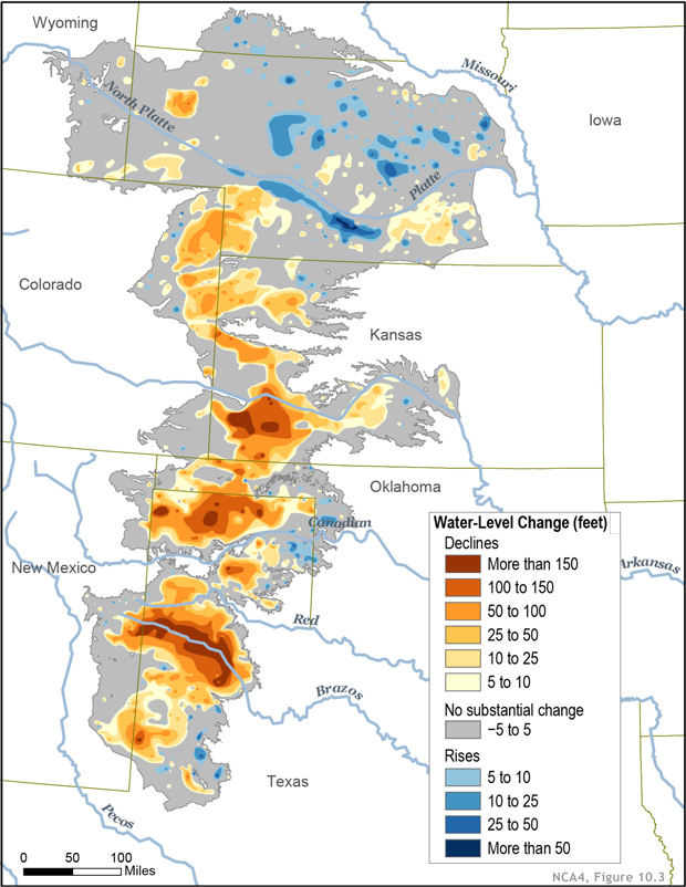
As a consequence of sustained overdraft for several decades (see Figure 44 above), water levels in the aquifer have dropped substantially, by more than 100 feet in many areas (Figure 48). Over half of this decline has occurred since 2000. Water level declines are not evenly distributed, however. The highest rates of decline are focused in the southern reaches of the aquifer system, where recharge rates are low and irrigation demand is highest. In the northern portions of the aquifer system, water level declines are considerably smaller – and in some cases, the water table has actually risen – primarily due to locally higher recharge focused along the Platte River (Figure 48).