Unit 1: Fresh Water: Scarcity or Surfeit?
Unit 1: Fresh Water: Scarcity or Surfeit?
Overview
Water is often called the “Elixir of Life.” We refer to Earth as the “Blue Planet” because of its abundance of liquid water; indeed, NASA’s search for life on other planets starts with the search for water. While its importance for sustaining life is perhaps common knowledge, the extent to which we depend on water in every aspect of our everyday lives and activities is less obvious. In this course, we will explore these facets of water’s impact on human society. We begin with an overview and discussion of the underpinnings of water use, occurrence, and movement. We then explore the many and profound consequences of human manipulation of water; the ability to reroute, store and transport water is one of the very things that has allowed human civilizations to thrive, yet has also led directly to a complex and broad-ranging relationship with this most essential of substances. Water pervades almost every aspect of our existence, including food production; the manufacture of goods and development of new technologies; transportation and energy generation; human health via its use for sanitation, the conveyance of waste, and control on the distribution of water-borne diseases; and the sustenance of ecosystems on which we often depend but do not realize. Not only is water needed for you to be here and to produce your breakfast this morning, but the computer you are using to read this course’s modules, the electricity needed to turn on your computer, the steel and fuel needed to transport you to/from school all required even more water!
Through its importance in these areas, it is perhaps unsurprising that water allocation and policy lie at the heart of economic and political tensions between communities, states, and nations. As populations in many water-stressed areas continue to grow, and in the face of climate changes that affect where and when water may be available in the future, these challenges continue to mount.
We begin this course by providing an outline of water resources on a global basis—where resources are abundant or limited and why. We first ask questions regarding the "value" of water and consider whether having access to fresh (uncontaminated) water for drinking and other household uses is a fundamental right as opposed to water being a commodity subject to profit-taking. In other words, is water a resource that is subject to privatizations and price fluctuations, or should water be provided by benevolent governments at a reasonable cost? In addition, we are concerned with projected population growth, its regional distribution, and resulting demands for water in the future. This helps us appreciate the two-way relationship between water and human society: how water availability and quality affect economic opportunities and human well-being, and how human activity affects water resources.
A major consideration is why some regions have a surplus of water and others have less than necessary to support local populations in various activities. In order to understand this, we need to examine the operation of Earth's climate system in some detail: the roles of global wind systems, proximity to an ocean, and topographic features (especially mountain belts) in determining patterns of rainfall, a first-order control on water availability. This involves discussion of the global "hydrologic cycle" that reflects the cycling of water from the ocean to atmosphere to land and its ultimate return to the sea. We also outline some of the important properties of water that determine its behavior in the climate system, flowing water, and sustaining life.
Modules
Unit Goals
Upon completion of Unit 1 students will be able to:
- Describe the two-way relationship between water resources and human society
- Explain the distribution and dynamics of water at the surface and in the subsurface of the Earth
- Interpret graphical representations of scientific data
- Identify strategies and best practices to decrease water stress and increase water quality
- Communicate scientific information in terms that can be understood by the general public
- Predict how the availability of and demand for water resources is expected to change over the next 50 years
Unit Objectives
In order to reach these goals, the instructors have established the following learning objectives for student learning. In working through the modules within Unit 1 students will be able to:
- List the primary reasons that most population centers developed near major rivers or other surface water bodies.
- Provide examples of consumptive and non-consumptive, and direct and indirect water uses.
- Compare the amounts used by the various end-users of water, both in the U.S. and globally.
- Identify regions of critical water stress at present and those anticipated 20 and 40 years into the future.
- Identify possible solutions to anticipated water shortages.
- Discuss issues surrounding the debate about public access to (clean) freshwater.
- Identify the unique physical properties of water that contribute to its fundamental role in driving Earth Systems.
- Quantitatively compare fluxes of water in the hydrologic cycle.
- Assess the relationship between precipitation, topography, and location in the U.S. and globally.
Module 1: Freshwater Resources - A Global Perspective
Module 1: Freshwater Resources - A Global Perspective
While only just beginning this course, you likely already appreciate that water is a precious commodity. For example, a human can survive at least three weeks without food, but can go only about three days without drinking water (or water-based liquid) before dehydration becomes a medical emergency (see the U.S. National Library of Medicines article, Water in Diet [3]. Nonetheless, in the U.S., we commonly take access to quality drinking water for granted, not to mention the availability of water for all other important activities including the production of food and energy. And, this water presently comes to most people in the U.S. at a very low cost—just cents per gallon. We are, of course, privileged relative to other regions of the world, some of which do not have sufficient fresh water resources and where people may not even have access to safe drinking water supplies.
In this module, we will examine the distribution of freshwater resources, the major uses of water, and present and anticipated future demand for water, globally, as the human population increases. We will explore the question as to whether water has a value greater than presently appreciated and whether it will always be readily available to us. For example, you may already know that the western U.S. is experiencing a severe shortage of water as the result of prolonged drought in that region. Is this an anomaly, or might we expect longer-term shortages there and elsewhere in the U.S. and globally as the result of climate change?
Goals and Objectives
Goals and Objectives
Goals
- Describe the two-way relationship between water resources and human society
- Explain the distribution and dynamics of water at the surface and in the subsurface of the Earth
- Communicate scientific information in terms that can be understood by the general public
- Interpret graphical representations of scientific data
- Identify strategies and best practices to decrease water stress and increase water quality
- Predict how availability of and demand for water resources is expected to change over the next 50 years
Learning Objectives
In completing this module, you will:
- Analyze the relationship between land use and access to fresh water
- Calculate the population that can be supported by a finite water source
- Evaluate possible solutions to anticipated water shortages
- Evaluate whether access to clean water is a basic human right, or if it should be treated as a commodity
- Distinguish between direct and indirect water use
- Record and analyze your own personal water usage
- Compare your own personal water use habits with those of your peers and others worldwide
The Value of Water
The Value of Water
Does water have value?
Water is essential to life – both as a basic human need for survival and as an “ingredient” in almost everything we do, from food production to manufacturing to power generation. As we will explore in more detail in Module 2 next week, precipitation and evaporation – and thus water availability – are unevenly distributed around the globe (Figure 1). This also varies seasonally. Figure 1 shows the average global distribution of precipitation for January; to see an animation over the course of the year, check this out:

There are obviously some areas of the world that are wetter than others, and these patterns are persistent throughout the year (i.e. the deserts of the American southwest, Northern Africa, and Western Australia are perennially dry; whereas equatorial central America, Africa, and Indonesia are wet). This uneven distribution of water resources lies at the root of many topics we’ll cover in this course, because it is a primary driver of human activity, ranging from population dynamics to types and locations of particular industries, to power generation, to politics. For example, take a look at the maps in Figures 1 and 2. Are there areas of the world that are persistently wetter or drier than others?


Activate Your Learning
1. List 3 areas/regions that are persistently dry based on the animated map shown above.
2. List 3 areas/regions that are persistently wet.
3. Inspect the freshwater availability map shown in Figure 2. Provide 2 examples of areas of water scarcity that “map” to areas where precipitation is low.
4. Identify 2 areas that are characterized by low precipitation, but apparently are not faced with severe water scarcity. Provide a hypothesis as to why you think this is the case.
As we’ll see in Module 2, water is transported around the Earth by the hydrologic cycle, in which solar energy drives evaporation of water from the oceans and land surface. This water condenses in the atmosphere to form clouds and eventually to fall as precipitation. Much of that precipitation flows as surface water in rivers and streams. Some of it also infiltrates or percolates into the soil and rock, and becomes groundwater. Surface water constitutes the primary source of water for human activity – it is relatively clean, easy to obtain and move, and constantly replenished (barring prolonged dry periods; as we will discuss in Modules 4 and 8-9). Groundwater constitutes another important source of water for human activity. Although the total volume of groundwater held in fractures and pore spaces in the subsurface is large, it is replenished and flows under natural conditions far more slowly than surface water. Additional energy is required to extract groundwater, because it must be pumped from the subsurface, in some cases hundreds of feet or more. For these reasons, groundwater is generally a secondary source of water, in cases where surface water is not readily available or cannot fully meet demand.
Food for Thought
List at least 2 problems or issues (these can be political, economic, health-related, etc…) that might arise from the unequal geographic distribution of water resources.
Global Freshwater Resources
Global Freshwater Resources
Water use and treatment
Once taken for human use, water generally follows a path described in Figure 3 below. After undergoing treatment and distribution, it is used. In the broadest sense, water is constantly being re-used. Water that is taken from rivers or streams for domestic, industrial, or agricultural use was most likely also used by communities or farms up-stream, and subsequently treated and discharged. Over even longer timescales, the water in streams, lakes, and groundwater is the same water that has ever been on Earth – and those same molecules have undoubtedly cycled through many plants and animals before we were even around!
Depending on the nature of water use, it may be re-captured after treatment (“recycled water”) for re-use. As we will see later in the semester, this re-use of water resources is one strategy to cope with water scarcity. The recycled water, depending on its quality, can be used for irrigation (i.e. for parks or golf courses), or for domestic supply. Once the water leaves the “use” loop, it is treated and discharged, typically into surface water bodies. In some cases, the treated water may be used to recharge aquifers instead, either through induced recharge systems or at a smaller scale via passive filtration through soils – for example in leachfields. The discharged water, after mixing with water in the river, stream (or aquifer), becomes a water source for downstream or down-gradient users.

Activate Your Learning
1. Do you know the source of domestic or municipal water in your hometown? If yes, what and where is it? If no, does it surprise you to realize that you don't know where your drinking water comes from?
2. Do you suppose that any of that water is used and then treated by others before being taken for your use?
3. Take a look at figure 3 above. Had you thought about your water as a substance that has a “life cycle” and is constantly being used, treated, released, and re-used? If not, does the idea make you uncomfortable?
Water and Population Centers
Water and Population Centers
Some cities are sited in areas where water is available - or was at the time they were settled - including Las Vegas, Los Angeles, Chicago, St. Louis, and Pittsburgh (Figure 4). In some cases, and as we will discuss in detail in later modules in the course, rapid development and growing demand can outpace the original and limited water source for a city or region, leading to a vicious cycle of water acquisition, growth enabled by water availability, and subsequent water stress.


Many of America’s major manufacturing centers (i.e. the rust belt) are located in areas where major rivers and canals provided a means for transport of raw materials and goods, power generation, water supply for processing and cooling, and conveyance of waste. At small scale, harnessing hydropower was accomplished by mills; at larger scales in modern dams, it is through hydroelectric power generation. Major rivers also provide the water supply for irrigation-based agriculture in some areas, where precipitation is not sufficient or consistent enough to support crops.

Indeed, for these reasons, rivers in many parts of the world are considered the “lifeblood” of society (Figure 6). For example, the Nile River valley in Egypt comprises ~5% of the land area, yet is home to nearly the entire population of 78 million, with a population density among the highest in the world (more than 1000 people per square km). Despite the obvious connection between water availability and human needs, the story of water resource distribution and population growth is not that simple! In some cases, major engineering projects in which millions of acre-feet of water are moved across states or continents have allowed cities and irrigated agricultural regions to flourish in water-scarce parts of the world. In others, major dams or new water sources (i.e. deep groundwater, reclaimed water, or desalination) have provided a means for cities to prosper in unlikely places. For example, take another look at Figure 4 above. The concentration of nighttime lights provides a reasonable proxy for population density. In many parts of the U.S., they follow the water: along the St. Lawrence, girdling the Great Lakes, and along the Mississippi River. Yet other major population centers have sprung up in perennially dry regions, mainly in the deserts of the southwest: Los Angeles, Las Vegas, Tucson, and Albuquerque.
Learning Checkpoints
1. Inspect Figures 4 and 5 and compare the two maps. Note 3 major cities that are near large water sources (rivers or lakes). View Figures 4 and 5above.
2. List 3 cities or regions of high population density that are not near major water sources, and/or lie in areas of low precipitation.
3. Do you know anyone who lives in one of these dry areas, or have you thought about moving there?
Water Quality and Human Health
Water Quality and Human Health
The distribution of water-rich and water-poor regions is of course not the whole story – access to clean water isn’t just about the amount of water that falls as precipitation. It’s also about the infrastructure needed to obtain, treat, transport, and deliver potable water. And that’s just the water supply. Disposal and sanitation of dirty water are equally important and require a means of transporting waste away from the distributed sources, collecting it and treating it, and discharging it safely. Ideally, both supply and waste conveyance systems should also be monitored for performance and for their impacts on water quality.
In some areas, water is plentiful, but access to clean water is not (Figures 7-8). The converse is also true, mainly in developed nations where water projects, desalination, or dams provide a water supply to regions that receive little precipitation. There is also a clear distinction between access to clean water in rural and urban areas (Figure 7), wherein access in rural areas, even in developed nations, lags behind that in urban areas.

Learning Checkpoint
1. What is the primary trend shown in Figure 7 above, with respect to urban vs. rural areas?
2. Is there a major difference in access to clean water supply and sanitation when comparing developed and developing nations?
3. Which is the bigger difference – urban vs. rural, or developed vs. developing nations?
4. Do you find your answer to question #3 surprising – or is it what you had expected?
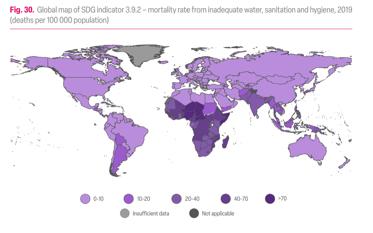
Access to clean water differs between rural and urban areas, and between developed and developing nations. In general, in rural areas, even in developed nations, access to water and sanitation lags behind that in urban areas. Globally, the areas with the poorest access to clean drinking water are in equatorial and sub-Saharan Africa, and parts of South America and southeast Asia (Figure 8).
One might imagine that access to clean water and sanitation would be strongly correlated with water-related illnesses and death. For example, compare the maps in Figures 8 and 9.

Learning Checkpoint
1. Compare the maps in Figures 8 and 9. Is there a correlation between access to improved water and water-related illness? Note two areas where there is a correlation, either positive or negative. See Figures 8 and 9 above.
2. Based on Figure 8 and the distribution of water availability, do you think that these problems are related to water scarcity, or more related to water treatment and infrastructure?
Water Usage: What and Where?
Water Usage: What and Where?
How much water do we use, and for what? Water “permeates” almost every aspect of our lives (no pun intended!). Some uses of water are obvious – for example, municipal and domestic supply used for drinking, cleaning, flushing and watering. Others are less obvious, such as water used for irrigation to grow produce, grains, or feed. The water needed to raise livestock is one step further removed, since the water “used” to produce the product includes the water that must go into growing feed. Yet other uses of water are even less visible, for example for refining fuels, cooling for thermo-electric power generation, and the manufacturing of almost everything in our day-to-day lives.;
Because the types and scales of water use vary widely – from domestic wells that pump at a few gallons per minute, to allocations of major rivers in billions of gallons, the units of measurement used for water management also span an enormous range (see Units).
Water Use
Water Use
How much and for what purposes?
Globally, there is a widely varied usage of water, as a result of differing total populations and population densities, geography and climate (i.e. water availability), cultures, economies, lifestyles, and water use and reuse efficiency. This can be described both in terms of total water abstraction from surface water and groundwater sources and as per capita water withdrawal. It can also be divided to consider the end uses (for example, as percentages of the total use), or to consider the source of the water. Each of these facets of water use illuminates different aspects of the “water story”.
In many industrialized nations, the dominant water uses are for industry (including thermoelectric power generation, manufacturing, etc…) and agriculture (Figures 10-11). In contrast, domestic and municipal water use generally constitutes less than 15-30% of the total. In developing nations, this is somewhat different – total water use is smaller, less is used for industry, and the proportion used for domestic water supply is larger.
In the U.S., the average per capita use of domestic or municipal water (i.e. the most direct uses – those that would be measured by the water meter at your home) is about 215 m3 per person per year, equivalent to 156 gallons per day (as of 2002). For comparison, the total abstraction of water from surface and groundwater sources in the U.S. is about 1700 m3/person/yr, or 1230 gallons per day. The difference in these numbers represents the large proportion of water that goes to so-called “indirect” uses: food production, manufacturing, power generation, and mining, among others.
In contrast, in sub-Saharan Africa, total water use is less than 200 m3 per person per year (less than 12% of water use in the U.S.). Total abstractions in Western Europe are about 600 m3 per person per year, about 850 m3 per person per year in the Middle East; and 1150 m3 per person per year in Australia. Among those nations with the highest water use, agriculture accounts for anywhere from <40% of use (U.S.), to 67-81% (India and China), to as much as 96% (Pakistan). Industrial use (including power generation) ranges from over 80% of total water use to less 1%. In the U.S. water use for power generation is near 50%; in China, it constitutes 25% and in India about 5%. Germany, Russia, Canada, France, and much of Western Europe use around 60% of withdrawn water for power generation. Municipal and domestic water use typically constitutes about 10-20% of the total and varies little among the worlds most populous countries (Figure 9). You can explore these patterns on your own via a useful interactive plotting engine at Gapminder. [11]
It is important to note that because many products are imported or exported across state and national borders, the total abstractions of water in a given place do not necessarily map to the distribution of water “consumption” there. Consider tomatoes that are transported from California to Massachusetts. The water withdrawal from rivers and aquifers needed to grow the tomatoes would appear on California’s “water tab”, but the eventual use of that water would be elsewhere. The same goes for agricultural and industrial products exported internationally. This flow of indirectly used water, embedded in products, is termed virtual water, and is defined as the amount of water used in generation of the product, or alternatively, the amount of water that would be needed to generate the product at the site where it is ultimately used. It is “virtual” because the water use is indirect; it is required to make or grow the item but is not actually physically contained in the item or transported with it.
Consumptive vs. Non-consumptive Use
Another important aspect of water use is the degree to which the water is available for recycling and/or reuse (Figure 12; cf. Figure 2). For some water uses, including industrial or domestic applications, the wastewater is captured, treated, and may be reused. These are termed nonconsumptive uses. For example, water used in homes is, for the most part, recaptured for treatment and discharged to surface water or groundwater systems – or for recycling of supply. In this sense, the water is not removed from the system (i.e. not “consumed”). In other applications, the water is effectively removed from the Earth’s surface environment and is not available to be re-captured. These are consumptive uses. Examples include water used for agriculture, which is mostly transpired by plants or evaporated and thus transferred to the atmosphere, or thermoelectric power generation, in which much of the water also evaporates (think of the steam you may have seen rising from power plants – this is consumptive water use, in action!).
Learning Checkpoint
1. Describe the difference between consumptive and non-consumptive water use. Provide an example of each.

Click here for a text description


Click here for a text description

Click here to expand for a text description of Figure 13
Learning Checkpoint
1. Based on Figures 10-13, what are the two largest uses of water in the U.S.?
2. Have the dominant uses of water in the US changed much in the past 50 years? If so, how?
3. Note three regions or countries where the dominant water use is for agriculture (look at Figure 12). Note three where it is for industry. Is this what you would have expected?
4. How much water do you think you use per day for household or domestic activities (e.g., washing dishes, laundry, showering, cooking, drinking)?
Supply and Use on Multiple Scales: Units of Water
Supply and Use on Multiple Scales: Units of Water
Units of measurement: volumes, fluxes, and concentrations
The uses of water for human activity vary immensely, and as a result, water resource management covers a wide range of temporal and spatial scales. In some cases, the timescales are short and volumes relatively small (i.e. domestic pumping of several gallons per minute, over timescales of minutes or hours). At the other extreme, water allocations for states or municipalities are often considered in the context of average annual flows in the billions of gallons. Because so many different scales of measurement are used to describe water flux or discharge (volumes of water) and flow rates (the velocity of flow), it is important to have some facility with the various units of measurement and get a sense for their relative magnitudes.
As one example, the total fluxes of water through river systems – commonly used to define allocations of water for states or nations - are measured and reported in acre-feet. This is a unit of water volume equal to the amount of water that covers an area of one acre, one foot deep. One acre-foot is equivalent to 325,851 gallons (see summary of unit conversions from the U.S. Geological Survey [14]), and is often considered as the amount of water needed for a family of four for about one year.
As we’ll discuss in Module 3, over shorter timescales, river discharges are reported in units of cubic feet per second (cfs), cubic meters per second (m3/s), or gallons per minute (gpm). As one example, on average, Spring Creek carries about 50 cfs at Houserville, PA; this increases downstream to about 90-100 cfs at Axemann as the creek is fed by springs and small tributaries. Short-lived peak discharge may exceed 500 cfs after storm events. For comparison, the flow of the Mississippi River at St. Louis, MO is typically about 400,000-600,000 cfs; in major floods the discharge is over 1,000,000 cfs. The flow rates of rivers and groundwater, as we will see in Modules 3-4 and 6, are reported as a velocity - units of length per time. These measures represent the velocity of the water itself, or of an object (stick, boat, person, etc…) carried by the river or stream.
Yet other key quantities in hydrology are reported in units of an equivalent depth (or length) per time. For example, rainfall rates are described in units of inches, cm, or mm per hour (for individual storm events) or per year (i.e. annual average precipitation). Evaporation rates are reported in the same way – but of course, represent water transport in the opposite direction (up!). The total volume of water these represent depends on the area over which they occur.
The Geographic Distribution of Water Uses
The Geographic Distribution of Water Uses
A deeper look: the geographic distribution of water uses
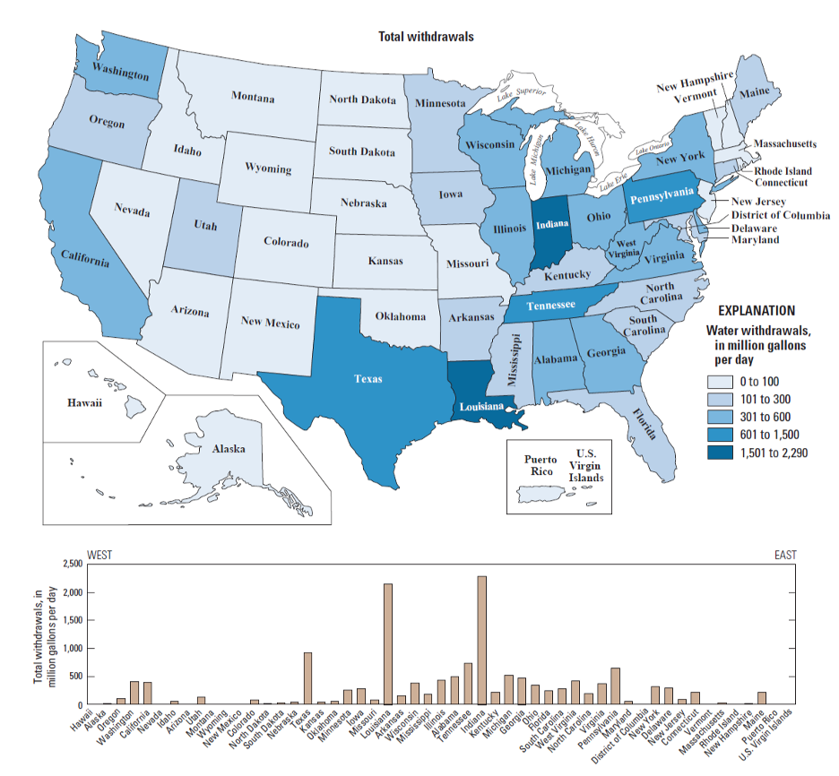
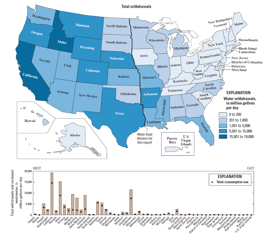
It is also instructive to look in more detail at the distribution of different water uses. For example, in the U.S., industry is concentrated East of the Mississippi, mainly in the “steel belt” (also known as the “rust belt”) and in Texas and Louisiana (primarily related to oil and gas extraction) – and thus water use for industry is as well (Figure 14). It’s worth considering whether this pattern is ultimately rooted in the timing of settlement and westward expansion in the U.S., availability of fuel (i.e. coal), or availability of water sources and rivers as a means of transportation for goods and raw materials. The pattern of water withdrawal for agriculture in the US is even more dramatic (Figure 15). Large agricultural water withdrawals from surface water and groundwater are dominantly West of the Mississippi. This is evident from a state-by-state map view and shown even more clearly when plotted simply from West to East (Figure 15, bottom panel).
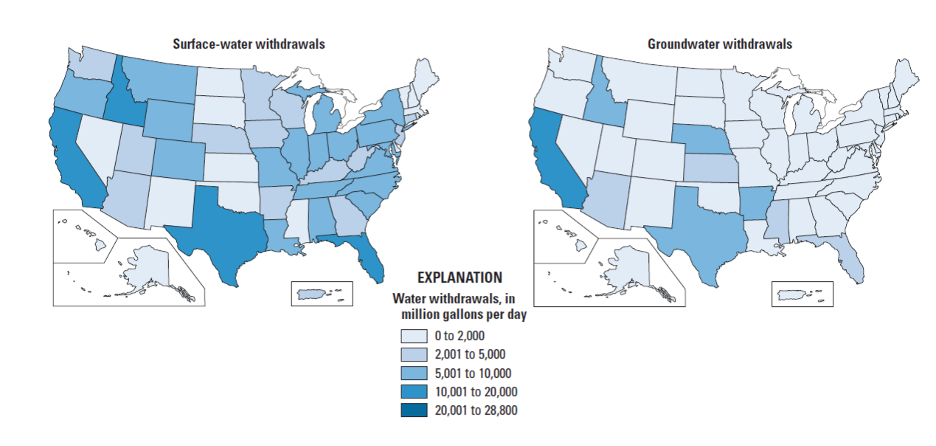
The source of the water we use also provides clues about where water may be most readily available, and/or where typical rainfall and snowmelt cannot meet demand. Inspect the maps below (Figure 16). Surface water withdrawals are spread more or less uniformly across the U.S., and reflect overall water use reasonably closely. This is influenced in large part by total population, energy production, and industrial and agricultural activity (i.e. CA, TX, NY, and FL are the most populous states). However, groundwater withdrawals (obtained by pumping at wells) are a good indication that surface water flows alone are not sufficient to meet demand.
Demand for Water
Demand for Water
As shown in the Freshwater Resources section, water demand varies by culture and country, while water availability is dependent on climate and geography (see also Module 2). Some areas of the world are already experiencing freshwater shortages and/or their water supplies are unsanitary as the result of improper treatment of waste and inadequate infrastructure to transport and store potable water. The combined specters of climate change and rapid population growth create uncertainty in planning future water supplies.
Future Demand for Water
Future Demand for Water
What will the future bring?
What will the future bring? Good question, right? How can we gauge what water demand and availability will be in the future, particularly with projected large increases in population and potential climate change superimposed? Not to alarm you, but to inform you, we will go through the exercise of making such projections, both for the U.S. and, on a more limited basis, for the world. What do we need to know for making such estimates? First, let's jot down some ideas. Then we will continue the process below.
Food for Thought
1. What do you think we would need to know in order to predict future demand for water? Take a minute to jot down what you think one would need to take the first crack at this.
First, here is an expert opinion as to how the future will go…
In Human Population and the Environmental Crisis Ben Zuckerman and David Jefferson write: “At a low population density, a society may be able to derive its water from rivers, natural lakes, or from the sustainable use of groundwater. As the population grows, so does the volume of water needed (we will assume demand is proportional to population size). Moreover, levels of waste discharge into the environment will grow as the population rises. Thus, the available unmanaged supplies deteriorate at the same time that demand on them is increasing…A destructive synergy is at work: population size affects the water resource in a manner that is not one of simple proportionality.”
What was it Yogi Berra (N.Y. Yankees catcher and later Manager) infamously said…"It's tough to make predictions, especially about the future." Well, that is a truism, but let's see what projections are being made regarding future population growth, because, clearly, that's one of the inputs we need to determine potential future water use globally.The present global population (as of 2024) is approximately 8.05 billion people. Interestingly, the top three countries, in terms of population, are China, India, and, yes, the United States, in that order (Figure 17). But, by 2050 the global population is estimated to be 9.7 billion people by the United Nations—a staggering 20% increase in the next, say, 26 years! So, at the minimum, if we assume that water use will increase linearly on a per person basis, we would expect that this rate of growth will require 20% more fresh water by 2050. Is that a problem? Do we have excess capacity to supply this water?
Population Growth vs. Water Needs
Population Growth vs. Water Needs
Do we have excess capacity to supply this water? That is an important question, but you have probably already determined that the real issue is where the population growth occurs and what water resources are available there. The major growth is projected to occur in developing countries (Figure 17). African nations are likely regions for greater than average growth. Interestingly, much of Africa is estimated to have significant groundwater resources (BGS, 2013) that could be developed if necessary. In fact, Nigeria is projected to surpass the population of the U.S. by 2050 (Figures 17-19). One must examine the population density and rate of projected growth vs. water needs. In addition, climate change impacts must be considered.


Learning Checkpoint
1. What is the relationship between Total Fertility and Per Capita Income shown in Figure 19 above?
2. Why might this be an important consideration when considering future demand for water?
Increased Impacts of Climate Change on Demand
Increased Impacts of Climate Change on Demand
We would probably be better off examining the impacts of climate change on water availability that would increase "water stress," then compare these stresses with those caused by increasing demand, either by population growth in a given region (personal or agricultural demands) or increased water usage resulting from new demands (e.g., energy production) (Figure 20). A number of studies have predicted water supply vs. water demand relationships resulting from climate change. A study by MIT (Massachusetts Institute of Technology) researchers (Schlosser et al., 2014) compared the potential impacts of climate change, on the basis of projected greenhouse gas emission increases in a complex Earth-system model, on water stress in 282 assessment regions (large or multiple watersheds) globally, holding demand constant, to the potential impacts of population growth in the same regions.


They found that, in most regions, projected population growth with increased demand to 2050 was the greater stressor. These researchers use a Water Stress Index (WSI) defined as WSI = TWR/RUN+INF (TWR is total water required for a given watershed region, i.e. all consumptive uses, RUN is available runoff within the watershed, and INF is inflow to the watershed from adjacent regions. The cutoffs used for interpreting water stress are: WSI<0.3 is slightly exploited, 0.3≤WSI<0.6 moderately exploited, 0.6≤WSI<1 heavily exploited, 1≤WSI<2 overly exploited, and WSI≥2 extremely exploited as originally set out by Smakhtin et al. (2005).
It appears that a substantial proportion of Africa, all of the middle East, India, and central Asia will see increased water stress in the next few decades, largely due to projected population increases. Even the southwestern U.S. is projected to experience expansion and intensification of water stress, but, in this case, mostly as the result of climate change and longer-term drought. Interestingly, the major central U.S. groundwater source, the Ogallala Aquifer, does not appear to be a candidate for significant stress except at its southern end in Texas. However, other studies (see Module 7) suggest that depletion of this aquifer will be more severe.
Possible Solutions for Meeting Water Demand in Stressed Regions
Possible Solutions for Meeting Water Demand in Stressed Regions
There are a number of possible methods to enhance supplies of fresh water, each of which has an economic, political, and/or environmental impact.
Learning Checkpoint
1. Provide three examples of potential ways to increase fresh water supplies.
Some of these strategies have been alluded to previously (e.g., encouraging transfers from agricultural use to drinking water supplies). Water storage behind dams is an old strategy and problematic in a number of ways (see Module 6), including high costs, environmental impacts, and political issues that arise when major rivers flow through multiple countries. Nonetheless, there is still major proposed and ongoing dam building in China and other countries.
Groundwater banking is a newer strategy that requires replenishment of aquifers with treated wastewater and/or with runoff available during times of excess. Costs are associated with treating, impounding, and injecting the water (see Module 7). This will mainly benefit regions with significant groundwater resources.
Recycling and reuse are gaining support with successful projects in the U.S. and elsewhere. Penn State University recycles and reinjects nearly 98% of its treated wastewater and has done so since the 1960s. Orange County, CA, has another successful system (see Module 8). Such systems must overcome consumer opposition, however, because of the perception that consumers will be drinking, well, toilet water! Nonetheless, the water quality in such systems is as good or better than that in municipalities that draw water from rivers downstream from other municipalities that discharge treated wastewater into the same river. Another form of reuse is to employ "gray" water (only partially treated) for irrigation of golf courses in arid to semiarid, water-stressed regions. Las Vegas, NV, has implemented such a system, coupled with the removal of water-hungry turf, for which the economics work and conservation is encouraged.
Desalination may be a last resort because of the costs of energy required to remove salts from seawater or water pumped from saline aquifers in non-coastal regions. However, in water-poor but hydrocarbon-rich middle-Eastern countries the economics may support the desalination of seawater. Alternative energy sources (e.g., solar) or emerging processes such as chemical reverse osmosis may be economical in the future as they become more efficient and less costly. And, of course, if water is deemed to have significant value in the future, the high costs may be more acceptable.
Finally, there are still proposals to import or export water from regions replete with fresh water resources (e.g. Alaska) to severely water-stressed regions (e.g. India). However, the costs of transporting such a commodity across the oceans would appear to exceed the value of that water at its terminus.
All of these strategies will be explored in later modules in more detail.
Pricing Water
Pricing Water

Does water have value? If so, how do we set a price for it? And, if we agree that individual access to fresh water is a basic human right or expectation globally (is this generally agreed?), how do we treat water as a commodity? Do we really pay what water is worth?
Pricing Varies
Pricing Varies
You are likely all too familiar with bottled water—that convenient liter-sized plastic bottle containing some sort of water, commonly tap water, or filtered spring water, sometimes treated…it appears that, in the U.S., we pay for the convenience of "grab-and-go." For that convenience, we typically pay about $4/gallon, more than we presently pay for a gallon of gasoline! In most municipalities; however, the cost of water delivered in pipes to taps in homes costs far less ($0.003-0.006/gallon). survey by CircleofBlue.org for 2019 water pricing in 30 cities across the U.S. found an average increase of 3.2% in monthly bills for a family of four using an average of 100 gals/day each (12,000 gals/mo or 45.4 m3/mo) from 2018 to 2019, costing an average of $72.93 a month.
Monthly rates for some representative municipalities are shown in the table below, based on data in the CircleofBlue.org 2014 survey and information from water authority websites for some municipalities not covered in that survey (Pittsburgh, PA and State College, PA).Note the large range in rates that do not seem to make sense geographically. For example, arid Phoenix, AZ has the lowest rate, with Las Vegas, NV not far behind, whereas high precipitation, seemingly water-rich regions such as Seattle, WA and Atlanta, GA top the rate list. Note that Los Angeles, CA, Phoenix, AZ, and Las Vegas, NV all depend on Colorado River water, although Los Angeles also draws on northern California sources and all require significant transport infrastructure. So, in part, this disparity in rates results from the costs of maintaining infrastructure and the numbers of households served, as well as the local abundance of water.
| Municipality (city, state) | Monthly rate (12,000 gals) | Percentage change (2014-2013) |
|---|---|---|
| Phoenix, AZ | $38.75 | 0 |
| Chicago, IL | $39.72 | +14.9 |
| Las Vegas, NV | $42.27 | +2.8 |
| State College, PA | $47.40 | 0 |
| New York, NY | $57.28 | +5.6 |
| Philadelphia, PA | $65.88 | +5.0 |
| Los Angeles, CA | $75.98 | +14.5 |
| Atlanta, GA | $91.92 | 0 |
| Seattle, WA | $98.77 | +9.3 |
| Pittsburgh, PA | $100.81 | ? |
Chicago, IL, for example, has nearby Lake Michigan as a source and a large number of users and its rates are relatively low. Little State College, PA has a significant, sustainable groundwater resource (see Module 6), even though the user base is relatively small. Many municipalities have higher rates because they are financing necessary improvements in infrastructure, which can be quite costly.
Municipalities have adopted different methods for scaling water prices. Some, such as Philadelphia and Detroit, provide cost reductions for larger users (decreasing block), some, including New York, have uniform pricing, whereas others, such as Las Vegas and Atlanta, have implemented tiered pricing (block increases) that encourage conservation while trying to maintain the user base. The objective of all municipalities is to sustain income and provide for future infrastructure requirements.
Internationally, pricing varies even more than in the U.S. Figure 22 illustrates average water prices (Kariuki and Schwartz, 2005) and the impact of non-public water suppliers on the cost to the consumer. Where public utilities are not available, the cost to the consumer can be a factor of 10 higher. In part, this occurs because of increases in cost to the water supplier to purchase water from a public or private supplier because of the large volumes purchased with prevailing block pricing increases. Figure 23 shows the step increases for several African and Indian cities. Recall that the average family of four in the U.S. would use about 45 m3/month, but average usage is probably much lower in many developing nations with lower standards of living. Step increases in block pricing appear to be a fair method of pricing to allow low cost for low-volume users and encouraging conservation by imposing higher costs for larger-volume users.


The Water and Energy Nexus
The Water and Energy Nexus
Considerations of water pricing are complicated because of the multitude of factors that must be taken into account. These include availability and dependability of water supply locally, state of the distribution infrastructure, and the distribution and size of the user base. Dependability is related to climate impacts, such as prolonged droughts that deplete water reserves. A recent study (Watergy Nexus: The Complex Relationship and Looming Crisis Between Our Thirst For Water and Our Hunger for Energy [18]) highlights an additional factor—the amount and cost of energy to acquire, transport, and treat water. This study argues that the cost of energy (usually electricity, but including fuel if the water is trucked in) must be considered in pricing water. The study uses data for 2013, a year of severe drought in much of the western and central U.S. to show how water prices should be adjusted to guarantee supply and cover costs of acquisition. Although the U.S. Geological Survey indicates that the average energy required to provide 1000 gallons (1 kgal) of water is 1.9kWh of electricity, water-stressed regions such as northern California (3.5 kWh/kgal) and highly stressed southern California (11.1 kWh/kgal) require far more (Figure 24). However, the study suggests that municipalities are not taking this factor into consideration in providing a durable and resilient water supply. During times of water stress, municipalities may have trouble meeting costs, and begin to examine other strategies, such as privatization. Of course, when water availability becomes restricted, costs can go up as in California with severe drought conditions (e.g., see the news article In dry California, water fetching record prices [19] about California water pricing: ).

Learning Checkpoint
1. What factors drive water pricing?
Privatization
Privatization
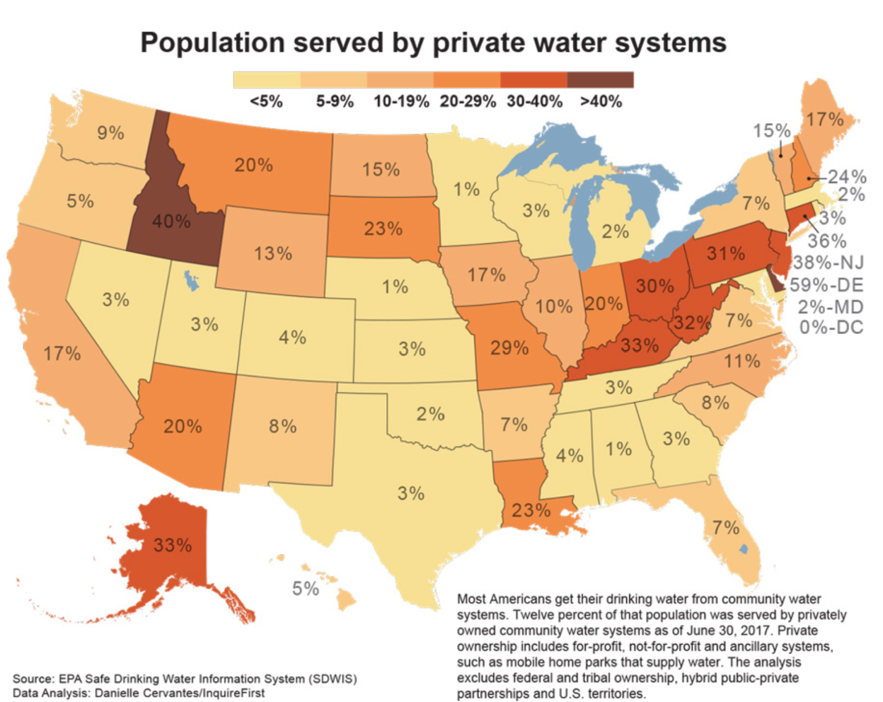
Cash-strapped municipalities with failing water systems might be tempted to contract with private companies to manage their water and sewer systems. Economic drivers, such as the collapse that occurred in 2008, affect users ability to pay for public water systems. In the U.S., about 20% of water supplies are privatized at present. In evaluating this option, one must keep in mind that corporations are for-profit entities, and will need to recoup the full costs of providing water while adding a margin for profit to benefit the corporation and/or their stockholders. Public utilities can be held responsible for controlling costs and providing clean water supplies, whereas it is more difficult for the public to do so for private companies.
There are a number of examples where privatization has apparently failed consumers. Pushed by the costs of renovating their failing water supply infrastructure, Atlanta, GA, for example, handed over control of their water system to United Water, which took over in 1999, with a 20-year contract. Atlanta had long-deferred most maintenance because their revenue was insufficient to cover the full cost of providing service, and because of rapid population growth and their aging system, expansion and improvement were required. Their sewage system was more of a problem than the water supply system, and they were being sued under the U.S. Clean Water Act for that problem as well.
But, in 2003, the city of Atlanta withdrew from the agreement because a number of issues with United Water (see What Can We Learn From Atlanta's Water Privatization [21] for the full story), which included costs, viewed as excessive, and poor performance in maintenance, meter installation, and bill collection.
The situation in Detroit has been much in the news of late (for example – see this MSNBC article, Detroit residents and national allies protest water shutoffs [22]). As a result of the economic downturn, the Detroit Water and Sewer Department has recently gone on a campaign to force users to pay their outstanding water bills with the threat of cutoffs. In addition, the city of Detroit is pursuing the possibility of privatizing its water and sewer systems. Although clearly having its own perspective and position, an interesting argument against water privatization in Detroit [23] is found on The Blue Planet Project website. One common argument against privatization is the rapid increase in the costs of water to consumers. Of course, in many cases, this may occur because the public purveyor was not charging for the full cost of providing the water in the first place.
Michigan lawmakers propose that water bills are capped at 3% of households income and $2 added to bills that can afford to make up for lost income. Claiming that shutting off water is a human rights violation. Read more here. [24]
A 2022 Cornell Chronical story explains that private ownership had the largest impact on annual water bills, which averaged $144 higher in privately owned systems than in public sector systems. Low-income households served by private operators spent 4.4% of their income on water service, about 1.5 percentage points more than in communities with public ownership.
Module 2: Climatology of Water
Module 2: Climatology of Water
Overview
In this module, we will investigate the underlying causes of variations in precipitation on Earth, with a specific focus on large-scale climate belts and the role of mountain ranges in affecting the distribution of rainfall (and snow). The goals of the module are to develop a quantitative understanding of the physical processes that control the distribution of precipitation, and which ultimately govern regions where water is abundant and where it is scarce, both across the U.S. and globally. As part of this, you’ll develop facility with the concepts of relative humidity, saturation, water vapor content in the air, and how these vary with changes in temperature - all of which play a key role in determining when and where precipitation falls.
Goals and Learning Objectives
Goals and Learning Objectives
Goals
- Explain the distribution and dynamics of water at the surface and in the subsurface of the Earth
- Interpret graphical representations of scientific data
Learning Objectives
In completing this module, you will:
- Identify the unique physical properties of water that contribute to its fundamental role in driving Earth Systems
- Identify U.S. and global precipitation patterns by reading precipitation maps
- Quantitatively compare fluxes of water in the hydrologic cycle
- Calculate relative humidity, and use it to quantitatively explain Earth's first-order patterns of precipitation
- Assess the relationship between precipitation, topography, and location on the globe
Unique Properties of Water
Unique Properties of Water
Water has some unusual properties that most of us do not really appreciate or understand. These properties are crucial to life and they originate from the structure of the water molecule itself. This sidebar will provide an overview of water's properties that will be useful in understanding the behavior of water in Earth's environment.
The Configuration of the Water Molecule
The Configuration of the Water Molecule
A molecule of water is composed of two atoms of hydrogen and one atom of oxygen. The one and only electron ring around the nucleus of each hydrogen atom has only one electron. The negative charge of the electron is balanced by the positive charge of one proton in the hydrogen nucleus. The electron ring of hydrogen would actually prefer to possess two electrons to create a stable configuration. Oxygen, on the other hand, has two electron rings with an inner ring having 2 electrons, which is cool because that is a stable configuration. The outer ring, on the other hand, has 6 electrons but it would like to have 2 more because, in the second electron ring, 8 electrons is the stable configuration. To balance the negative charge of 8 (2+6) electrons, the oxygen nucleus has 8 protons. Hydrogen and oxygen would like to have stable electron configurations but do not as individual atoms. They can get out of this predicament if they agree to share electrons (a sort of an energy "treaty"). So, oxygen shares one of its outer electrons with each of two hydrogen atoms, and each of the two hydrogen atoms shares it's one and only electron with oxygen. This is called a covalent bond. Each hydrogen atom thinks it has two electrons, and the oxygen atom thinks that it has 8 outer electrons. Everybody's happy, no?
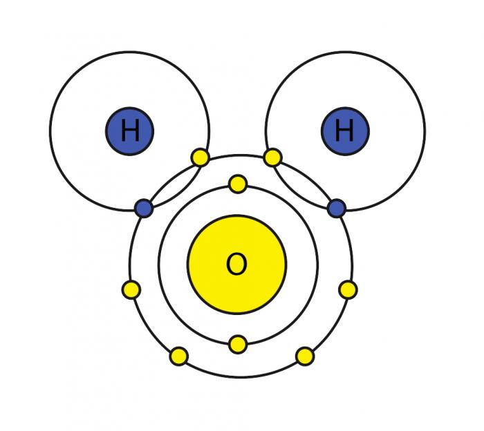
However, the two hydrogen atoms are both on the same side of the oxygen atom so that the positively charged nuclei of the hydrogen atoms are left exposed, so to speak, leaving that end of the water molecule with a weak positive charge. Meanwhile, on the other side of the molecule, the excess electrons of the oxygen atom, give that end of the molecule a weak negative change. For this reason, a water molecule is called a "dipolar" molecule. Water is an example of a polar solvent (one of the best), capable of dissolving most other compounds because of the water molecule's unequal distribution of charge. In solution, the weak positively charged side of one water molecule will be attracted to the weak negatively charged side of another water molecule and the two molecules will be held together by what is called a weak hydrogen bond. At the temperature range of seawater, the weak hydrogen bonds are constantly being broken and re-formed. This gives water some structure but allows the molecules to slide over each other easily, making it a liquid.
The Structure of Water: Properties
The Structure of Water: Properties
Studies have shown that clustering of water molecules occurs in solutions because of so-called hydrogen bonds (weak interaction), which are about 10% of the covalent water bond strength. This is not inconsiderable and energy is required to break the bonds, or is yielded by the formation of hydrogen bonds. Such bonds are not permanent and there is constant breaking and reforming of bonds, which are estimated to last a few trillionths of a second. Nonetheless, a high proportion of water molecules are bonded at any instant in a solution. But this structure leads to the other important properties of water.
We will consider, for the purposes of this course, only six of these important properties:
- Heat capacity
- Latent heat (of fusion and evaporation)
- Thermal expansion and density
- Surface Tension
- Freezing and Boiling Points
- Solvent properties
As mentioned above, these properties have importance to physical and biological processes on Earth. Effectively, large amounts of water buffer Earth surface environmental changes, meaning that changes in Earth-surface temperature, for example, are relatively minor. Thus, the high heat capacity of water promotes continuity of life on Earth because water cools/ warms slowly relative to land, aiding in heat retention and transport, minimizing extremes in temperature, and helping to maintain uniform body temperatures in organisms. However, there are other effects of water properties as well. Its low viscosity allows rapid flow to equalize pressure differences. Its high surface tension allows wind energy transmission to sea surface promoting downward mixing of oxygen in large water bodies such as the ocean. In addition, this high surface tension helps individual cells in organisms hold their shape and controls drop behavior (have you seen "An Ant's Life"?). Also, the high latent heat of evaporation is very important in heat/water transfer within the atmosphere and is a significant component of transfer of heat from low latitudes, where solar energy influx is more intense to high latitudes that experience solar energy deficits.
Video: Water - Liquid Awesome: Crash Course Biology #2 (11:16)
Take a few minutes to learn why water is the most fascinating and important substance in the universe.
Heat Capacity
Heat Capacity
Water does not give up or take up heat very easily. Therefore, it is said to have a high heat capacity. In Colorado, it is common to have a difference of 20˚ C between day and night temperatures. At the same time, the temperature of a lake would hardly change at all. This property originates because energy is absorbed by water as molecules are broken apart or is released by molecules of water associating as clusters.
Video: Heat Capacity of Water (01:13)
Take a few minutes to watch the video below to help you understand heat capacity.
Latent Heat and Freezing and Boiling Points
Latent Heat and Freezing and Boiling Points
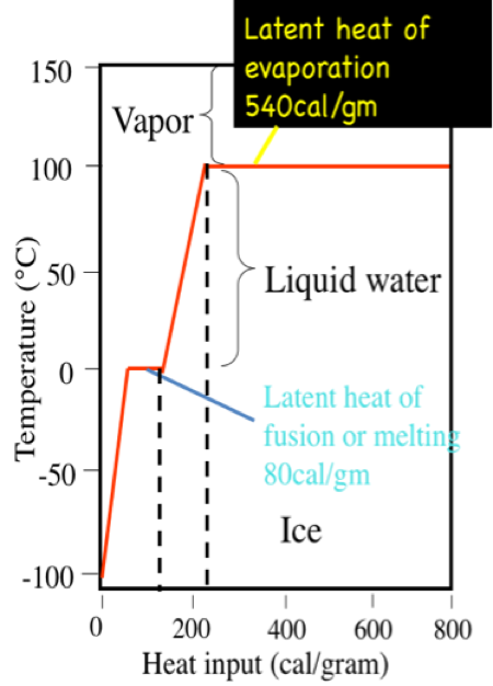
A calorie is the amount of heat it takes to raise the temperature of 1 gram (0.001 liters) of pure water 1 degree C at sea level. It takes 100 calories to heat 1 g. water from 0˚, the freezing point of water, to 100˚ C, the boiling point. However, 540 calories of energy are required to convert that 1 g of water at 100˚ C to 1 g of water vapor at 100˚ C. This is called the latent heat of vaporization. On the other hand, you would have to remove 80 calories from 1 g of pure water at the freezing point, 0˚ C, to convert it to 1 g of ice at 0˚ C. This is called the latent heat of fusion.
Interestingly, the latent heat and freezing and boiling points are controlled by the way water molecules interact with one another. Because molecules acquire more energy as they warm, the association of water molecules as clusters begins to break up as heat is added. In other words, the energy is absorbed by the fluid and molecules begin to dissociate from one another. Considerable energy is required to break up the water molecule clusters, thus there is relatively little temperature change of the fluid for a given amount of heating (this is the heat capacity measure), and, even at the boiling point, it takes far more energy to liberate water molecules as a vapor (parting them from one another). On the other hand, when energy is removed from water during cooling the molecules of water begin to coalesce into clusters and this process adds energy to the mix, thus offsetting the cooling somewhat.
Click here for a text description
Thermal Expansion and Density
Thermal Expansion and Density
When water is a liquid, the water molecules are packed relatively close together but can slide past each other and move around freely (as stated earlier, that makes it a liquid). Pure water has a density of 1.000 g/cm3 at 4˚ C. As the temperature increases or decreases from 4˚ C, the density of water decreases. In fact, if you measure the temperature of the deep water in large, temperate-latitude (e.g., the latitude of PA and NY) lakes that freeze over in the winter (such as the Great Lakes), you will find that the temperature is 4˚ C; that is because fresh water is at its maximum density at that temperature, and as surface waters cool off in the Fall and early Winter, the lakes overturn and fill up with 4˚ C water.

However, as dissolved solids are added to pure water to increase the salinity, the density increases. The density of average seawater with a salinity of 35 o/oo (35 g/kg) and at 4˚ C is 1.028 g/cm3 as compared to 1.000g/cm3 for pure water. As you add salts to seawater, you also change some other properties. Incidentally, increasing salinity increases the boiling point and decreases the freezing point. Normal seawater freezes at -2˚ C, 2˚ C colder than pure water. Increasing salinity also lowers the temperature of maximum density. This effect also helps explain why you are supposed to add salt to ice when making ice cream or to add salt to water when cooking spaghetti (although, in this case, the effect on boiling point is minor and the added salt is mainly for flavor).
When water freezes, however, bonds are formed that lock the molecules in place in a regular (hexagonal) pattern. For nearly every known chemical compound, the molecules are held closer together (bonded) in the solid state (e.g., in mineral form or ice) than in the liquid state. Water, however, is unique in that it bonds in such a way that the molecules are held farther apart in the solid form (ice) than in the liquid. Water expands when it freezes making it less dense than the water from which it freezes. In fact, its volume is a little over 9% greater (or density ca. 9% lower) than in the liquid state. For this reason, ice floats on the water (like an ice cube in a glass of water). This latter property is very important for organisms in the oceans and/or freshwater lakes. For example, fish in a pond survive the winter because ice forms on top of a pond (it floats) and effectively insulates (does not conduct heat from the pond to the atmosphere as efficiently) the rest of the pond below, preventing it from freezing from top to bottom (or bottom to top).
If water did not expand when freezing, then it would be denser than liquid water when it froze; therefore it would sink and fill lakes or the ocean from bottom to top. Once the oceans filled with ice, life there would not be possible. We are all aware that expansion of liquid water to ice exerts a tremendous force. Have you or a family member (you wouldn't admit to this would you?) ever left a full container of water with a tight-fitting lid (or even a can of soda?) in the freezer? In other words, 10 cups of water put into the freezer is going to turn into 11 cups of ice when it freezes (oops). The force of crystallization of ice is capable of bursting water pipes and causes expansions of cracks in rocks, thus accelerating the erosion of mountains!
A rough sketch of water molecules in ice crystal form is below.

Surface Tension
Surface Tension
Next to mercury, water has the highest surface tension of all commonly occurring liquids. Surface tension is a manifestation of the presence of the hydrogen bond. Those molecules of water that are at the surface are strongly attracted to the molecules of water below them by their hydrogen bonds. If the diameter of the container is decreased to a very fine bore, the combination of cohesion, which holds the water molecules together, and the adhesive attraction between the water molecules and the glass container will pull the column of water to great heights. This phenomenon is known as capillarity. This is a key property that allows trees to stand high, for example, because surface tension stiffens stems and trunks. Plants "wilt" because they are unable to acquire sufficient water to maintain the required surface tension. And, of course, water droplets (rain) and fog condensing as droplets on surfaces are a function of water's surface tension. Without this property, water would be a slimy coating and cells would not have shape. Surface tension decreases with temperature and salinity.
Video: Amusing Surface Tension Experiment (02:39)
Please take a few minutes to watch this amusing video to learn more about the surface tension of water.
The Universal Solvent
The Universal Solvent
This is, of course, another key property of water because more substances dissolve in water than any other common liquid. This is because the polar water molecule enhances "Dissolving Power." Dissolution involves breaking "salts" into component "ions." For example, NaCl (common salt) breaks down into the ions Na+ and Cl- because of the attraction for ions (atoms or groups of atoms with a charge) to water molecules is high.

Cations, such as Na (Sodium) have a net positive charge, whereas anions (such as Cl, Chloride) have a net negative charge. There are many individual elements and compounds that form ions. Thus, water can hold considerable concentrations of various chemical species depending on their particular properties. Note how the water molecules surround the individual ions, keeping them isolated from other ions in solution. This occurs until the capacity of water to isolate the ions is exceeded, at which point the solution is "saturated" with those ions and cannot dissolve more (salt will begin to precipitate—form a solid).
Learning Checkpoint
Water Distribution on Earth
Water Distribution on Earth
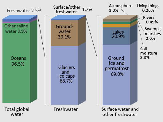
Where is water distributed on Earth?
Earth is often called the “Blue Planet”, because of its abundance of liquid water. As we’ve already covered in Module #1, this water is distributed in the oceans, ice caps and glaciers, surface water (streams, lakes, and rivers), groundwater, soil moisture, the atmosphere, and in biomass. However, these reservoirs of Earth’s water are not static; water is constantly fluxing between them. We see this transport of water every day, for example in the form of flowing rivers, rain and snow, and groundwater springs.
Systems Thinking and the Hydrologic Cycle
Systems Thinking and the Hydrologic Cycle
Throughout this course, we will be dealing with complex systems and “Systems Thinking”. What is Systems Thinking, you may ask? According to Peter Senge, author of The Fifth Discipline Fieldbook, “Systems thinking is a way of thinking about, and a language for describing and understanding, the forces and interrelationships that shape the behavior of systems”. Some systems are very complex, but all systems can be simplified to help understand the relationships between systems components. Systems can be "modeled" to help investigate their dynamics. We do not expect you to become system modelers, per se, but simple models can begin to help you understand how changes in one parameter might influence changes in another. Let's consider a simple system in which we have a bathtub, fed by a faucet, and drained at its lower level. We could diagram this simple system as follows…

In this system there is a reservoir (the bathtub), an input (the faucet), and an output (the drain). The relationships in this system are simple and, hopefully, intuitive. If you want to run water into the tub for a long time to keep it quite warm, but not have it run over, what are your choices? You could keep the drain closed and run a very slow trickle of warm water into the tub from the faucet, letting it fill gradually, or, you could fill the tub quickly to some level, then open the drain to allow water to leave the tub at the same rate as it is being added to prevent further rise in the water level. Cold water is more dense than warm, so perhaps cooler water would drain preferentially and this would keep the tub water warmer overall. You could also evaluate the time it would take to fill the tub, or drain it, knowing the tub volume (gallons), the maximum input rate through the faucet (gallons/minute), and the maximum drain rate (gallons/minute).
Learning Checkpoint
Let's try a couple of simple model calculations to get you thinking about systems dynamics. First, we should establish some volumes and rates for this simple system. The tub (reservoir) will hold 30 gallons of water. The input and output values are outlined below:
1) If the faucet (input) will supply 3 gallons of water per minute, and the drain is closed (no output), how long will it take to fill the tub to the brim with water if the tub is empty to begin with?
2) If the faucet supplies 3 gallons per minute, the tub is empty to begin with, but the drain allows 3 gallons per minute to leave the tub, how long will it take the tub to fill?
3) If the faucet supplies 3 gallons per minute, the tub is empty to begin with, and the drain allows 1 gallon per minute to escape, how long will it take to fill the tub?
Hydrologic Cycle
Hydrologic Cycle
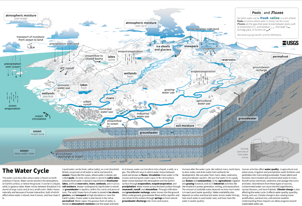
The movement of water between these reservoirs, primarily driven by solar energy influx at the Earth’s surface, is known as the hydrologic cycle.

The hydrologic cycle is a conceptual model that describes the fluxes of water between the oceans, surface water bodies (lakes, rivers, and streams), groundwater in subsurface aquifers, the atmosphere, and the biosphere. One important aspect of the cycle is that no water is gained or lost: water moves between reservoirs but the total mass remains the same. Another way to say this is that the water that currently exists on Earth is the same water that has been here since the time the Earth formed. (Technically, there are small fluxes of water from the Earth’s interior to the surface and atmosphere through volcanism and venting, and small influxes of water from comets and debris, but these are negligible in comparison to the mass of water in the primary reservoirs shown above.)
Activate Your Learning
1. There are five processes that control the movement of water between reservoirs in the hydrologic cycle. Looking at Figure 6 above, what do you think they are? Name as many as you can.
The movement of water between reservoirs, or the “limbs” of the hydrologic cycle includes five primary processes:
- Evapo-transpiration: the movement of water from oceans or land to the atmosphere, through the combined processes of evaporation and transpiration. Evaporation and transpiration both involve a change in state, from liquid to vapor, which requires an input of energy. Evaporation is simply the change from liquid to vapor as a result of molecular motion, and is affected by temperature and ambient humidity. Transpiration is the movement of water to the atmosphere by plant respiration. In most terrestrial basins, transpiration is the dominant process by which water moves from the Earth’s surface to the atmosphere, whereas over lakes and the oceans, evaporation dominates.
- Precipitation: the movement of water from the atmosphere to the land surface or oceans, in the form of rain, snow, sleet, ice pellets, etc... Precipitation involves a change in state from vapor to liquid, known as condensation. This change in state releases heat energy. After precipitation falls on the land surface, it may flow into surface water bodies (lakes or streams), or percolate through soils and rock into the groundwater system.
- Runoff: the movement of water from the land surface to the oceans in streams or rivers.
- Infiltration: the percolation of water from the land surface or from surface water bodies through soils and into the subsurface. Water that infiltrates becomes part of the groundwater system, and is also known as groundwater recharge.
- Groundwater outflow, also known as subsea outflow: the seepage of water from the groundwater system directly into the oceans. The flux of groundwater outflow is the least constrained component of the hydrologic cycle, and is often estimated by balancing the other fluxes in the cycle.
Because the changes in state that accompany evaporation and precipitation also take in and release energy, the movement of water through the hydrologic cycle is paralleled by redistribution of heat and energy.
Uneven Distribution
Uneven Distribution
Why is water distributed unevenly across the Earth’s surface?
As you probably know, things are far more interesting than a hypothetical case of evenly distributed precipitation! Both precipitation and evaporation vary widely over the Earth’s surface. This unequal distribution of water on the planet drives a diversity in climate and ecosystems (or biomes); water availability for human life, industry, and agriculture; and is fundamentally and intimately tied to the history of politics, economics, food production, population dynamics, and conflict – both in the U.S. and globally.
The abundance of water in some areas and scarcity in others follows systematic and predictable patterns. As part of this module, we’ll explore the physical processes that shape the overall distribution of precipitation - and thus water resources.


Learning Checkpoint
Note: The questions below are not graded. They may show up as summative evaluation questions on mid-term or final exams.
1) Look at Figure 7 above. What is the annual mean precipitation in Southern Nevada?
- 32 in/yr
- greater than 80 in/yr
- 0 in/yr
- 4-8 in/yr
2) Look at Figure 7 above. What is the annual mean precipitation in Coastal Washington State?
- a. 32 in/yr
- greater than 80 in/yr
- 0 in/yr
- 4-8 in/yr
3) Why do you think Nevada and Eastern Oregon are deserts?
- a. They are far North of the equator.
- They are far from the ocean.
- They are in the rain shadow of mountains.
- They are subject to large annual temperature fluctuations.
- They are at high elevation.
4) Look at Figure 8. What do you think is the global pattern of precipitation?
- a. It rains most South of the equator.
- There is East-West "banding" of climate/precipitation.
- There is North-South "banding" of climate/precipitation.
- There is snow in the Southern Hemisphere year-round.
Note the contrasting patterns in the two images in Figure 8 above, based on global satellite coverage. Vegetation in the southern hemisphere, which has relatively more ocean area (and less land area) than the northern hemisphere, changes little seasonally, whereas vegetation distribution in the northern hemisphere undergoes large changes. Why is that? There are probably two impacts on vegetation distribution—precipitation and temperature. Examine the figure below that illustrates the available moisture seasonally (summer vs. winter) and compare to the distribution of vegetation for the same seasons. Think about the role of temperature, precipitation, and soil moisture (water availability to plants), as well as the availability of sunlight for photosynthesis. Yes, there is a more complex relationship between plant growth and other factors, but the hydrologic cycle plays a major role.


Relative Humidity
Relative Humidity
The explanation for spatial variations in precipitation centers on the concept of relative humidity. The relative humidity is the water vapor pressure (numerator) divided by the equilibrium vapor pressure (denomator) times 100%. The equilibrium vapor pressure occurs when there is an equal (thus the word equilibrium) flow of water molecules arriving and leaving the condensed phase (the liquid or ice). Thus there is no net condensation or evaporation (Alistair Fraser, PSU).
Now, if the water vapor pressure is greater than the equilibrium value (numerator is greater), there is a net condensation (and a cloud could form, say). And that is not because the air cannot hold the water, but merely because there is a greater flow into the condensed phase than out of it.
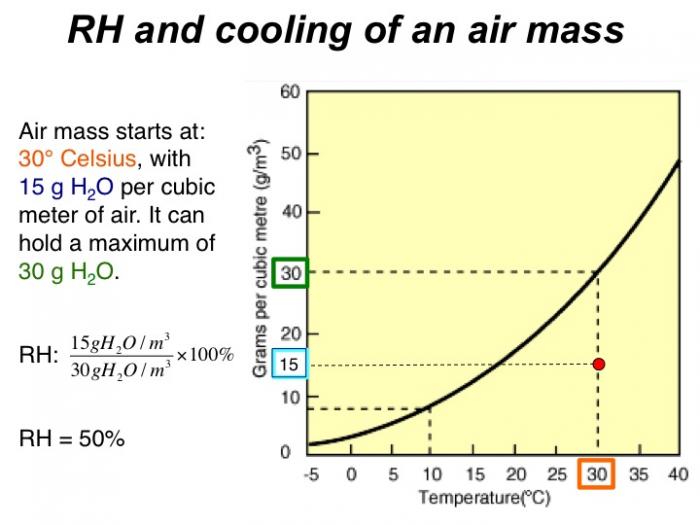
Relative humidity describes the amount of water vapor actually in the air (numerator), relative to the maximum amount of water the air can possibly hold for a given temperature (denominator). It is expressed as a percentage:
If the relative humidity (RH) is 100%, this means that condensation would occur. On a typical hot muggy summer day, RH might be around 60-80%. In a desert, RH is commonly around 15-25%.

One important consequence is that when air masses change in temperature, the relative humidity can change, even if the actual amount of water vapor in the air does not (the numerator in our equation, which is defined by the saturation curve, stays the same, but the denominator changes with temperature). Figures 11-13 below show an example of this process. As the air cools, the relative humidity increases. If the air mass were cooled enough to become saturated (hit the solid black curved line), condensation would occur. This temperature is called the dew point.


In the same way, changes in relative humidity occur when warm moist air is forced to rise or, conversely, when cool dry air descends. For example, when an air mass moves over mountains, it cools as it rises, and when it reaches the dewpoint, water will condense. This forms clouds, and if the air mass cools enough, the condensation becomes rapid enough to form precipitation.
The Orographic Effect
The Orographic Effect
To take the concept of relative humidity outdoors, let's consider why it rains in some areas and we have deserts in others. There are two primary reasons for this. Both are related to the transport, rise, and fall of air masses that lead to temperature changes, and ultimately in the amount of water vapor that the air can hold. These are the orographic effect, and atmospheric convection.
In both cases, cooling and warming of air masses occurs because they are forced upward or downward in the atmosphere. The decrease in air temperature with elevation is known as the atmospheric (or adiabatic) lapse rate, as shown below, and is related to decreasing air density and pressure with increasing altitude (as air rises, it expands due to decreased pressure, leading to lower temperature). A typical average lapse rate is around 7° C per km of altitude change. If an air mass begins rising and has not reached the dewpoint temperature, it follows a dry adiabatic lapse rate, with the rate of cooling due nearly entirely to decreasing pressure, as shown in Figure 14. Once the airmass temperature reaches the dewpoint during continued rise, water droplets begin to condense (forming clouds) and the airmass follows a moist adiabatic lapse rate (Figure 14), for which the rate of cooling with elevation decreases because of the addition of some offsetting heat to the airmass from the process of condensation (termed latent heat).

The orographic effect occurs when air masses are forced to flow over high topography. As air rises over mountains, it cools and water vapor condenses. As a result, it is common for rain to be concentrated on the windward side of mountains, and for rainfall to increase with elevation in the direction of storm tracks. With continued cooling past the dewpoint, the amount of water vapor in the air cannot exceed saturation, so water is lost from the air via condensation and precipitation.
On the leeward side of mountain ranges, the opposite occurs: the air descends and warms. As it does so, it is capable of holding more water vapor (recall the saturation line in the relative humidity plot above). However, there is no source of additional water, so the descending air mass increases in temperature but the amount of water vapor remains constant. Because the air has lost much of its original water content, as it descends and warms its relative humidity decreases. These areas are called rain shadows and are commonly deserts. You’ve probably noticed this same process in action when you heat your house or apartment in the winter – warming the cold air leads to dry conditions – one of the reasons people often put water pots or kettles on their wood stoves.
Orographic Effect In Action
The animation below shows an airmass trajectory superimposed on a Google Earth image of western North America. The point of this animation is to provide an explanation of the orographic effect and the changes in temperature and water content of an airmass passing over several mountain ranges. The animation shows the "rain shadow" effect that results in desert regions behind large mountain ranges. An inset graph at bottom right illustrates combinations of temperature (x-axis) and moisture content (y-axis) in grams per cubic meter of the air mass as it passes over various topographic features on the land surface.

Atmospheric Convection: Hadley Cells
Atmospheric Convection: Hadley Cells
There is a second, larger-scale effect that also plays a key role in the global distribution of precipitation and evaporation. Fundamentally, these patterns are also explained by the rise and fall, and cooling and warming of air masses – as is the case with the orographic effect – but in this case, their movement is a result of atmospheric convection rather than transport over topographic features.
As you have seen, there are regular climate and precipitation bands on the Earth – latitudes where most of the Earth’s tropical and temperature rainforests, deserts, polar deserts (also known as tundra) tend to occur. This global pattern – along with prevailing global wind patterns and storm tracks, are driven by atmospheric convection.
It all starts with solar radiation. Because of the Earth’s curvature, the tropics (between 23.5° N and S latitude) receive a larger flux of solar radiation per unit area on average than higher latitudes. Because the Earth’s axis is tilted, during Northern hemisphere summer, the peak influx of solar radiation occurs at 23.5° N latitude. During the Southern hemisphere summer, the maximum occurs at 23.5° S. (Incidentally, these latitudes define the tropics of Cancer and Capricorn.) Annually, the highest flux of solar energy per unit area occurs at the equator, as shown below.
As a result, the air around the equator becomes warmest. It holds quite a bit of water, too – based on the fact that, as you’ve seen above, warm air has a higher capacity to carry moisture.
Video Review: Global Atmospheric Circulation (2:24)
Take a few minutes to review the video below to help you understand Global Circulation a little better.
Energy Balance
Energy Balance


The differential heat input from solar radiation input and loss by infrared radiation is a critical part of maintaining equability (relatively low gradients in temperature from low to high latitudes) on the Earth. The energy balance figures indicate that above about 40 degrees North and South (e.g., the latitude of New York City) of the equator the loss of heat by radiation (infrared), on average, exceeds the input of heat from the sun (visible). What does that imply for our climate? One might think that this should result in permanent snow or ice above this latitude. Right? Indeed, during the last glacial epoch, about 21 thousand years ago, thick continental ice sheets extended to nearly 40 degrees North in North America (just north of I-80). But normally, because of the heat gradient created by the imbalance between solar input and infrared radiation, the atmosphere (and ocean) is set in motion to redistribute heat from low to high latitudes. Otherwise, the tropics would be excessively hot and the high latitudes excessively cold—at all times. Next, we will see how this circulation works.
Global Wind
Global Wind
As this warm air rises due to its lower density, it cools. Once it cools past the dewpoint, condensation occurs and clouds form. With continued rise and cooling, the air cannot hold the moisture and precipitation falls.
In response to that rising air, surface air must flow in to fill the vacated space. The rising air results in a low-pressure center. This is why when you hear about low pressure in the forecast, is typically associated with rising air masses and therefore with crummy weather. The air rushing in toward the equator defines the trade winds. These winds converge on the equator but blow to the West because of Earth’s rotation. This rotational effect is known as the Coriolis effect. We won’t get into that in detail here, but if you are interested, check out the video below.
Video: The Coriolis Effect (02:43)
These flows drive convection cells, with dimensions that are controlled by the viscosity and density of air, and by the thickness of the atmosphere. The air that rose from the equator flows North and South at the top of the cell and eventually descends at around 30° N or S latitude. As the cool, now dry air descends, it warms. Sound familiar?
Just as occurs when air descends on the leeward side of mountain ranges and causes rain shadows, the amount of water that the descending and warming air could hold increases. But there is no additional moisture to be found, so the actual amount of water vapor in the air mass remains more-or-less fixed. These descending limbs of the Hadley cells form high-pressure centers and would be regions where persistent dry conditions should prevail – leading to the Earth’s desert belts that include the Gobi, Sahara, Arabian, and the Australian Outback (not just a steakhouse!).
The equatorial convection cells are known as Hadley Cells. There are two more in each hemisphere, also driven by the uneven distribution of incoming solar radiation density; these are Farrell and Polar cells. Check out the diagram of this process below.

Global Wind Explained
Global Wind Explained
The illustration below portrays the global wind belts, three in each hemisphere. Note that the U.S. lies primarily in the Westerly Wind Belt with prevailing winds from the west. Each of these wind belts represents a "cell" that circulates air through the atmosphere from the surface to high altitudes and back again. The cells on either side of the Equator are called Hadley cells and give rise to the Trade Winds at Earth's surface. How do we explain this pattern of global winds and how does it influence precipitation?
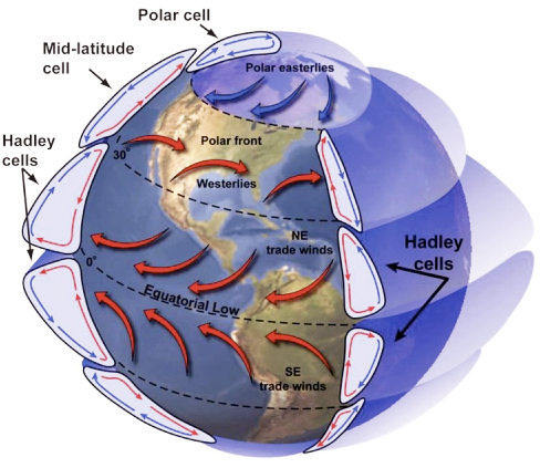
We'll start at Earth's equator, where solar radiation is the highest year around. Air near the equator is warmed and rises because it is less dense (mass/unit volume) than the air around it as shown in Figure 21 below.
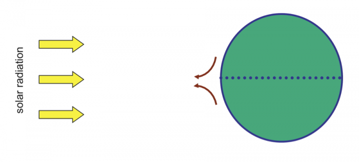
The rising air creates a circulation cell, called a Hadley Cell, in which the air rises and cools at high altitudes moves outward (towards the poles) and, eventually, descends back to the surface. The continual heating and rise of air at the equator create low pressure there, which causes air to move (wind) towards the equator to take the place of the air that rises. On the other hand, sinking air creates high pressure at the surface where it descends. A gradient of pressure (high to low) is formed that causes air to flow away from the high and towards the low pressure at the surface.


The Earth would have two large Hadley cells if it did not rotate. But, because it does rotate, the rotation of the Earth leads to the Coriolis effect. You should view the short video on this so-called "effect" or "force." (The Coriolis Effect [30]). Without going into detail as to why rotation creates this apparent force, the Coriolis effect causes winds (and all moving objects) to be deflected:
- to the right in the Northern Hemisphere
- to the left in the Southern Hemisphere
The Coriolis effect causes winds to deflect as they travel within circulation cells and results in the two large hypothetical Hadley cells breaking into six smaller cells, which looks something like the diagram below (and the first figure in this series).

Ok, so, we now have some idea about the origin of global wind systems that result from pressure gradients at Earth's surface. How does this produce precipitation, and where? Precipitation occurs where moisture-laden air rises, either by heating at the equator or by running up and over a more dense air mass. As the rising air cools its capacity to hold water decreases (relative humidity increases) and, at some point, saturation with respect to water vapor is reached. Then, condensation--clouds and rain!

The diagrams above and below portray just the Hadley cell circulation, that is driven by heating in the equatorial region. On the surface, wind moves away from high pressure (High) and toward low pressure (Low). Convergence occurs near the equator (winds blow in towards one another) and Divergence occurs under the descending air that forms high-pressure belts. The final figure (Figure 26) shows all six cells diagrammatically, along with the pressure variations at the surface of the Earth and zones of typical wet and dry belts. Note particularly the dry belts near 30 degrees North and South.

