EBF 200
Lesson 1 - Thinking About Economics
Lesson 1 Overview
Did you complete the course orientation?

Before you begin this course, make sure you have completed the Course Orientation in Canvas.
An Overview of Lesson 1
Did you ever wonder why engineers typically earn more money than short-order cooks, or how the price of gasoline gets established? Why is it that so many Americans drive to work, but lots of people in Britain take the train, and many Dutch ride their bicycles? Speaking of cars, why do we have so many choices when we want to buy a car, but so few choices if we want to buy cable TV or home Internet service? And why is it that if I want to buy a car, I have to go to a dealership, but I can buy a computer directly from Dell (although I don't have to)? On a more personal note, do you ever stop and think about what you choose to spend your money on? Do you choose to spend more of your income on entertainment than, say, a nicer car? Why don't you do both?
These are all questions that can be answered (or, at least, better understood) by using economic analysis. In this lesson, we will talk about some of the basic underlying principles that guide economics as a way of looking at the world.
What will we learn?
By the end of this lesson, you should be able to:
- list and describe the axioms that underlie the "economic way of thinking";
- describe the economic definition of scarcity;
- define what an "opportunity cost" is;
- tell the difference between a positive and normative question;
- list and describe what is contained in a property right.
- explain what economists mean by the terms "utility" and "monetization".
- What are Gregory Mankiw’s ten fundamental principles of economics?
What is due for Lesson 1?
This lesson will take us one week to complete. Please refer to Canvas for specific timeframes and due dates. There are a number of required activities in this lesson. The chart below provides an overview of those activities that must be submitted for this lesson. For assignment details, refer to the lesson page noted.
| Requirements | Submitting Your Work |
|---|---|
|
Reading: Chapters 1 and 2 in Gwartney et al., OR Chapters 1 and 2 in Greenlaw et al. |
Not submitted |
| Lesson Homework and Quiz | This will be submitted via Canvas |
Questions?
If you have any questions, please post them to the online discussion forum in Canvas.
A Desert Island Economy
I am tempted to start the course by trying to say "what economics is" and so on, but it is perhaps easiest to start with a simple illustration.
Imagine you are on a desert island. There are two things you can eat on this island: coconuts and fish. If you wish to survive, you spend all of the available daylight trying to catch fish or harvest coconuts from the palm trees. We can assume, for the time being, that all of your day is taken up doing one of these two things. You need to divide your day between gathering coconuts and catching fish since a diet of just one or the other is not healthy. Suppose you have 10 hours a day to work. It takes you one hour to catch a fish and climbing a tree to get a coconut takes half an hour. So, in 10 hours you can catch 10 fish, or you can gather 20 coconuts. You could also do a bit of both: maybe spend 8 hours fishing and 2 hours getting coconuts, which would give you 8 fish and 4 coconuts. After a few weeks on the island, you settle on a balance whereby you spend 7 hours a day catching fish and 3 hours harvesting coconuts. This gives you 7 fish and 6 coconuts per day. If you want more fish, you have to give up some coconuts, and if you want more coconuts, you have to give up some fish, because there are only a certain number of hours in a day, and you can't make more daylight!
Now, what if it turns out that you are not alone on this island. Suppose there is a person who happens to go by the name "Friday." He's been on the island a long time and has gotten good at fishing. It turns out that he can catch a fish in 20 minutes, but it also takes him half an hour to climb a tree and harvest a coconut. Friday has gotten into a routine where he fishes for 4 hours a day, catching 12 fish, and he harvests coconuts for 6 hours, getting 12 coconuts per day.
This is getting a little complicated, so we'll summarize:
- You: 7 fish, 6 coconuts per day.
- Friday: 12 fish, 12 coconuts per day.
- Total: 19 fish, 18 coconuts.

Now, let's suppose that one day, you and Friday meet up for the first time. After a bit of discussion, you start talking about food, and how much food you get each day. You both work 10 hours per day and get a total of 19 fish and 18 coconuts.
What if I said that it was possible for both of you to get more fish and more coconuts, and neither of you had to work longer hours? Is this magic? Well, not quite.
Let's say you decided to spend all of your day harvesting coconuts, meaning that you were able to get 20 in a day.
At the same time, Friday spends 8 hours fishing. He is able to catch 24 fish and gets 4 coconuts in the other two hours.
Now, between the two of you, you have 24 fish and 24 coconuts. You have more fish AND more coconuts
So, collectively, you are better off. However, neither of you likes the proportion of things you have yourself. You have too many coconuts and not enough fish. Friday does not have enough coconuts. What you can do then is make a trade. Let's say you trade away 10 coconuts in exchange for 10 fish. Now you have 10 coconuts and 10 fish. Friday has 14 coconuts and 14 fish.

Let's summarize:
- Before you meet, 7 fish and 6 coconuts.
- After you meet, 10 fish and 10 coconuts.
Friday:
- Before you meet, 12 fish and 12 coconuts
- After you meet, 14 fish and 14 coconuts.
So, after meeting, you both have more fish and more coconuts. How has this happened? Is this some kind of magic? As I said before, not quite.
The above story may seem a little simplistic - it is - but it powerfully illustrates some important topics that we talk about in the field of economics. What has happened? Well, the first thing that happened after the meeting of you and Friday is that you decided to specialize. You decided to do what you are good at - gathering coconuts. Friday concentrated most of his time on what he is good at - catching fish. By focusing on what you are each good at, you became more efficient. You then decided to trade. Specialization and trade made you both better off and made the sum of the two of you better off.
Complicated? Of course! So, let’s do some more examples.
Example: Comparative Advantage and the Robinson Crusoe Economy
- Robinson Crusoe is stuck on a desert island to fend for himself. He can gain two goods, fish and coconuts.
- In any one day, he can gain 0 coconuts and 8 fish, 1 C and 6 fish, 2 C and 4 fish, and so on down to 4 C and 0 fish. In mathematical terms, Rob can get , where C stands for coconut and F for fish (C and F non-negative). Rob maximizes his happiness, and let us assume (somewhat arbitrarily) that he chooses 3 C and 2 F.
| Rob's Choice | Coconuts | Fish |
|---|---|---|
| #1 | 0 | 8 |
| #2 | 1 | 6 |
| #3 | 2 | 4 |
| #4 | 3 | 2 |
| #5 | 4 | 0 |
What is Rob's opportunity cost of coconuts? 2 fish
What is Rob's opportunity cost of fish? 0.5 coconuts
Rob Meets Friday
It turns out that Friday is living on the other side of the island. Friday has a "production function" such that .
| Friday's Choice | Coconuts | Fish |
|---|---|---|
| #1 | 0 | 4 |
| #2 | 1 | 3 |
| #3 | 2 | 2 |
| #4 | 3 | 1 |
| #5 | 4 | 0 |
Living by himself, Friday chooses 2 C and 2 F.
What is Friday’s opportunity cost of coconuts?
Of fish?
Can Rob and Friday make each other better off?
YES, THEY CAN.
- Assume (for example) Friday makes only coconuts: 4C and 0F. Rob makes 1C and 6F. (So, they specialize.)
- Now together they have 5C and 6F - more than they had separately.
- Assume Rob trades 2.5 fish to Friday for 2 coconuts. Now, are they both better off?
- Rob now has 3C and 3.5F. Before he met Friday he had 3C and 2F. So, he is better off, since he is greedy, and therefore more goods are preferred to less.
- Friday has 2C and 2.5F. Before he met Rob he had 2 of each. So, he is better off.
- So, both Rob and Friday gain from trading – even though Friday wasn’t better than Rob at anything!
Note the 4 Step Approach
- Figure out each party’s opportunity cost.
- Figure out each party’s comparative advantage.
- Determine which good each party should specialize in, and determine production.
- Have the 2 parties trade to make each better off.
Remember, More is Better Than Less!
Example: Comparative Advantage Rosie and Donald
Rosie O’Donnell and Donald Trump are stuck on a deserted island. Rosie has the production function , where T is the production of turtles and B is the production of bananas. The Donald has production function . If they could not trade with each other, Rosie would choose to produce 3 turtles, and the Donald would produce 13 turtles.
Figure out a possible production/allocation system where both the Rosie and the Donald would be better off trading than not trading.
Rosie has the production function , which implies that each turtle cost 3 bananas. She chooses , which implies that , .
The Donald has production function , which implies that each turtle costs 1/6th of a banana. The Donald chooses , so, .
Turtles are much cheaper for the Donald rather than Rosie (1/6th of a banana vs. 3 bananas). So, Donald should trade turtles with Rosie for bananas.
Many trades/production decisions are possible.
Assume Rosie makes all bananas. Since for her, , she makes 20 bananas.
If Donald makes all turtles, he makes 25 turtles.
So, we now have .
Without trade , . So, now we have more production of each.
So, now assume that The Donald trades 6 turtles for 5 bananas.
The Donald now has , . Before, he had and . So, he is better off because he has more of both.
Rosie now has and . Before, she had , . So, she is better off.
Both parties gain from trading!
Practice Exercise
Eric and Rod are stuck on a desert island. There are two goods, fish (F) and coconuts (C). Eric has production function , and without trading chooses . Rod has production function and without trading chooses . Explain an arrangement that can make both better off. Make sure you don’t fall into the trap!
The same idea holds for more complicated scenarios involving more than two people and more than two goods. If people in a society decide to specialize and make a lot of what they are good at making, and then trade some of the things that they make for other things they want, then both they and the society they are part of will be better off. Or, as I will say a little later on, specialization and trade generate wealth for society.
This is perhaps not hard to understand. We all specialize in something and sell it and use the proceeds of that sale to buy other things. A university professor specializes in teaching students and generating research. The university pays the professor for this, and with his wages, he buys food, housing, transportation, clothing, leisure, and many other things. He is better off doing this than trying to make his own food, build his own house and manufacture his own car. A construction company might build a hundred houses a year, which is more than the owners of the company need. So, they sell some of those houses to buy the other things they need to live. This is how our society is organized.
As a society, we have much more wealth because we arrange our societies this way. Without trade (that is, buying and selling things), we would each have to be a fully self-sufficient unit, and each of us would have much less in such a world. We do not trade because we like each other or even care about each other - we usually don't even know the people we are trading with - but we do so because it is in our own best interest. This curious fact - a society of people, each acting in their own best interest (or out of selfish motives), leads to an increase in the wealth of society as a whole - was first written down and expounded upon by Adam Smith, the author of a book called The Wealth of Nations, which was written in 1776 and was the founding text of modern economic thought. We'll talk a bit more about Smith later.
Now, given this simple example as an introduction, we can move on to start talking about economics in a bit more of a formal and structured manner.
What is Economics?
Reading Assignment
Please note that we will not go into further detail in the course notes on budget constraints or production possibilities frontiers, and therefore this material will not be on any quizzes or tests.
Economics is a social science. What exactly does that term mean? "Social" means that is about examining the way the people organize their interactions with each other in societies. "Science" means that the "scientific method" is used as a way of thinking about and studying social organization. We have some other social sciences, such as sociology, anthropology, education, history, and law. These disciplines all look at different aspects of societies or examine them from a certain perspective. Economics is the social science that concerns itself with how people make consumption and production choices in a world of endless wants and limited means.
Economics is not an ideology or a set of political beliefs; it is merely one of the ways in which people try to understand the society we live in, and how it works. It is a way of looking at the world, what we call the "economic way of thinking." This has proven to be a useful tool for understanding and explaining a great deal of human behavior. It explains how people do many of the things they do, and why, and it allows us to predict, with a reasonable degree of confidence, what the effects of some action taken by a government or a group of individuals will be.
Note that I said, "reasonable degree of confidence." That could be taken as a set of meaningless weasel words, with terms like "reasonable" and "confidence" not being clearly defined. However, what I am trying to do when I make this statement is to avoid being too sure about our knowledge of the outcomes. While it is true that people behave in a way that is "generally" predictable, you must always remember that when we study societies, we are talking about people, and people do not uniformly behave in a predictable manner. In mathematical terms, there are too many variables, and we cannot isolate and correct them all. So, what I am saying here is the "soft-sell" on economics: it is a helpful and pretty reliable way of understanding the world, just not a perfect or strictly deterministic way. Note that the "economic way of thinking" has been applied to many other social science disciplines, most famously law and sociology, and it has done a great deal to explain behavior in these areas. If you are interested, you may want to read more about the works of people like Richard Posner in law and economics, and Gary Becker in sociology. Economics also has strong ties to the field of psychology. Several of the recent Nobel Prizes in economics have been awarded to scholars or teams studying economic behavior from a psychological perspective. This should be unsurprising: both disciplines have the goal of trying to figure out how and why people make the decisions and choices that they make.
A great many economics textbooks have been written, and they all strive to start at the same place, laying out what the "fundamental principles" are. One of the best attempts is by Gregory Mankiw, a professor at Harvard University and former chair of the President's Council of Economic Advisors. He has laid out a list of ten "principles of economics" that is broadly accepted as a good summary of the main points that I will try to make here.
Actually, it's more like "7 Principles," because the last three pertain to macroeconomic issues, which is an area of study that will not be addressed in this course. Instead, we will examine microeconomics, which is the study of individual economic actors: people, and firms, and their interactions in markets. Included as an agent in this study will be governments, which play a large role in the economic lives of every individual and every firm.
A good understanding of these seven points will provide you with a very solid grounding for how to think about economic problems throughout this course and throughout the rest of your lives. I will list them below, with some explication. Before I list them, I want to add three "axiomatic" statements that have to be considered before we move on. An axiom is an assumed statement, sort of a "first principle" that is not, or need not be proved. It is a basic understanding of how things happen.
Axiom 1: Things that we want to consume more of are called economic goods or, usually, just "goods". The opposite of a good is a "bad," which is something that we want less of. However, there are very few things that are universally bad - almost every economic bad is somebody else's good. For example, we might think of pollution from burning coal as bad, and it certainly has a detrimental effect on many people, especially those who live near power plants. But the more pollution a plant operator can put into the air, the more electricity he sells, and the more money he makes.
Axiom 2: All goods are scarce. It is important to understand what "scarce" means in this context. There are quite a few words that have one meaning when used in general conversation, and a narrower, more specific definition when used in economic analysis. In general usage, "scarce" usually refers to something that is in short supply, or is running out, or is hard to find. In economics, scarce simply means that something is not limitless. Another way of thinking about it is this: a good is considered scarce if we have to give something up to consume it. When viewed in this light, the phrase "all goods are scarce" makes a bit more sense. Bottles of orange juice or episodes of TV shows are not scarce in the general sense, but they certainly are in the economic sense.
Axiom 3: Wants are unlimited. This is perhaps a polite way of saying "people are greedy" in the sense that people almost always prefer to consume more goods than less. If they reach a limit to how much of some good they want to consume, it is not hard to find another good they would like to consume more of. It is important to consider that things like leisure, rest, and peace of mind can be seen as goods.
Now, moving on to Mankiw's list:
Principle 1: People face tradeoffs.
This means that we have to make choices in a world of unlimited wants and scarce resources. If you want something, you will have to give something else up. You have to make a choice. Perhaps, in a perfect world, we would not have to make choices – we could have all that we want without having to give up anything else, but this is not the world we live in. From the desert island example, we had a simple trade-off: if you wanted more coconuts, you had to give up fish, and vice versa. If you wanted more leisure time, you had to give up some food to get it.
Principle 2: The cost of something is what you give up to get it.
In everyday life, we think of costs generally in terms of money, or perhaps time or effort. However, whenever you make an economic choice, what you give up are all of the choices that you didn’t make. This is what we call an “opportunity cost.” Ask the average man on the street what the cost of a bag of Doritos is, and he will say “99 cents.” Ask an economist, and he will tell you “every other thing that I could have spent 99 cents on." Or maybe, “the most valuable thing I could have spent 99 cents on, but did not because I spent it on Doritos.” Needless to say, this causes a lot of people to avoid having conversations with economists at parties but, nonetheless, thinking about costs in this way helps us better understand economic decision making. This contains a secondary point: money is only a tool, a store of value or a method of accounting. Money is only basically good for one thing: exchanging for goods that we consume. So, the cost of one consumption choice is the most valuable consumption choice we could have had, but chose not to make. Likewise, the opportunity cost of an investment, of either time or money, is the best other investment we could have made with that time and/or money. For example, the opportunity cost of going to an 8 am class is probably an hour of sleep for most people. Once again, think back to the desert island economy: it took you an hour to catch a fish, or half an hour to get a coconut. So what was the cost of a fish? Well, you can look at it two ways: first, you could say that it cost you an hour. This is true, but, really, an hour was only good for one of two things: catching fish or harvesting coconuts. So, if you spent an hour catching a fish, you were giving up two coconuts. We say that the opportunity cost of the fish is two coconuts - 2 coconuts is what you have to give up to gain an extra fish.
Opportunity cost is all the other things you give up to get something else. For example, let’s say you buy a car for 25 thousand dollars. If you don't spend your money on buying the car, you could invest your money (for example: deposit it into a savings account and receive interest or buy stocks, ...). When you buy the car, you give up all the other things that you could have done with the 25 thousand dollars. In economics, you should consider all of those. For example, if investing the money would give you interest, then, the opportunity cost of buying the car would be 25 thousand dollars plus lost interest of given up investment.
Another example: When you are a full-time student, the opportunity cost would be: the tuition that you pay plus money that you could have made if you were working and not spending your time at school.
Another example: Let's assume you are living in Pittsburgh and you want to buy a TV. There is a store in Pittsburgh that sells the TV for 500 dollars. However, you find a store in New York that has a TV on sale for 300 dollars. But there is no shipping service. So, you need to go there and pick it up there. What would you do? The true cost of buying the TV from the store in New York is \$300 plus all the other costs that you don't need to pay if buy the TV from the Pittsburgh store. If you decide to buy the TV from New York:
- You need to rent a car (if you use your own car, you should consider the wear and tear costs of driving to New York and back).
- You need to pay for gas.
- If you work, you need to take a day off and lose the money that you could have earned.
Next is a short video with more explanation.
Video: What is Opportunity Cost? (2:45)
♪ [music] ♪
[Narrator] What is opportunity cost? Opportunity cost refers to the value a person could have received but passed up in pursuit of another option. So if you were to wait in line for free ice cream, you actually give up the opportunity to do something else with your time, like working at a job or reading a book. So that ice cream really isn't free. Economists even use the concept of opportunity cost to determine if people can benefit from trading with one another. Let's look at a simple example -- just two people, Bob and Ann, who produce just two goods, bananas and fish. Because of the concept of opportunity costs, Ann and Bob are worse off when they try to do everything themselves. Here's what Bob can do if he spends all of his time producing only one good. Bob can either gather 10 bananas, or he can catch 10 fish. And Ann can either gather 10 bananas or catch 30 fish. Bob has to choose to gather bananas or catch fish. When he chooses to gather 1 banana, he gives up 1 fish. In essence, Bob trades with himself. He can use that time to gather bananas or trade that time to catch fish, and the cost of that trade is 1 fish per banana. That's Bob's opportunity cost. The same holds true for Ann, but her cost of producing 1 banana is 3 fish. In the amount of time that it takes Ann to gather 1 banana, she could have caught 3 fish. She trades with herself 1 banana for 3 fish. So Bob only has to give up 1 fish to produce 1 banana, but Ann must give up 3 fish to produce 1 banana. Ann's opportunity cost of gathering a banana is higher than Bob's. If Ann and Bob are allowed to trade with one another, they may be able to gain from specialization if Ann focuses on catching fish, and Bob focuses on gathering bananas. Because our time is valuable, any decision we make has a cost. If we focus our time on tasks we're good at, like Ann and Bob, then we end up in a better position than if we try to do everything ourselves.
♪ [music] ♪
To learn more about the role of specialization in trade, click here. Or, to test your knowledge on opportunity cost, click here.
♪ [music] ♪
Still here? Check out Marginal Revolution University's other popular videos.
♪ [music] ♪
Principle 3: Rational people think at the margin.
“Thinking at the margin” means that we think about the next decision we need to make, and the incremental effects of that decision. Put another way, people have to be forward-looking, because the past is in the past, and nothing can be done to change it.
Principle 4: People respond to incentives.
I will talk about this in more depth in the next section when we address rationality and utility maximization. This principle is intuitively very obvious: every child understands the notion of the carrot and the stick: positive and negative incentives designed to modify behavior. A further examination of this topic leads us to discover that people usually act in their own best interest, so when governments design policies, they have to be sure that they are incentivizing the “right” behavior. An interesting topic has arisen recently: the Estate Tax, which is applied to inheritances, is set to be reinstated at the beginning of 2011 after having lapsed at the end of 2009. This means that a wealthy person dying a few minutes after the coming New Year will leave his or her heirs with a significantly larger tax bill than if he died a few minutes before midnight. Thus, the heirs perhaps have an incentive to see to it that a terminally ill parent dies a little bit earlier. This is what is called a “perverse incentive,” because our society generally frowns upon people trying to cause others to die earlier than they otherwise might. Whenever you participate in an economic transaction, it always helps to think about what incentives the other person in the transaction faces.
Principle 5: Trade can make everyone better off.
I might be inclined to make a stronger statement: that trade MUST make everybody better off, but we can go with Mankiw’s weaker statement for now. The fundamental notion behind voluntary trade is that each party is giving up something in exchange for something that they place a higher value upon. If this were not the case, the person would choose to not make the trade. For example, when I buy a bag of Doritos, the shopkeeper will voluntarily make the trade because I am paying him more money than he paid for the chips, so he’s better off, and I will voluntarily make the trade because I get more happiness from consuming the chips than anything else I could spend that 99 cents on. We’re both made better off by the transaction. We will look at applications of this notion in much more depth later on.
Principle 6: Markets are usually a good way to organize economic activity.
This is another statement that could be made a little more forcefully, but we can let it be. Markets refer to institutions (not just places) that allow people to voluntarily and willingly participate in trades to improve their lives. People sell their labor and brain power to firms, which use it to help them make profits for the owners of those firms. People use the money they earn to purchase goods and services to help them live their lives in a way that best makes them happy. In a truly free-market system, we have millions of individual, voluntary economic transactions taking place every day. In reality, sometimes (or, perhaps, always) markets do not work in this idealized manner, which leads to the next principle.
Principle 7: Governments can sometimes improve market outcomes.
When markets do not work well, we speak of “market failure” (there will be much more on this later in the course). Sometimes a government can intervene in a market, by setting rules or restrictions that enable a better outcome for society than would be obtained through an unfettered free market. Many people believe, for example, that product safety laws or workplace safety rules are unambiguous improvements upon unregulated outcomes. However, the government cannot fix every problem, and sometimes government intervention in a market can end up making things worse for society. This is what is called “government failure,” and we will also look at this in much more depth later on in the course.
The last three principles, which I will simply list below, pertain to macroeconomic issues that will not be addressed in this course.
Principle 8: A country’s standard of living depends on its ability to produce goods and services.
Principle 9: Prices rise when the government prints too much money.
Principle 10: Society faces a short-run tradeoff between inflation and unemployment.
Utility and Individual Rationality
As outlined in the previous section, we are trying to study why people make the economic decisions that they make. To try to understand this question, we assume that people do things that make them happy. This is not a difficult concept to understand: any time we are faced with a choice, there is an outcome that will make us happier than another outcome. Some choices are not very enjoyable, such as doing our laundry or paying our taxes, but we do so because the alternative will leave us with less happiness: most of us prefer clean clothes to dirty, and most of us prefer to not be hounded into court by the taxman.
Economists don't use the word "happiness," but instead have coined another term: "utility." You might think of a utility as the company that provides your electricity or drinking water, and these have the same root meaning derived from the word "use." In the economic context, think of utility as the use, the value of the use or the happiness derived from the use of some good. Basically, "utility" is the economic catch-all term for whatever benefit we get from the consumption of some economic good, or in a broader sense, the benefit we derive from the outcome of an economic decision.
So, if somebody gets utility from making a decision, and more utility (happiness) is unambiguously better than less, then we make the claim that people are "rational utility maximizers." That is, in every decision that we make, we think rationally about the outcomes and make the choice that gives us the most utility. This is a simple and elegant statement, and it lies at the foundation of modern western economic thought, but it is not completely uncontroversial or even all that uncomplicated. For example, many decisions are not simple yes/no or A/B choices. Sometimes there are many possible choices - indeed, there are usually many possible choices, and we don't always know which of those choices will make us happier for the simple reason that we cannot see the future with perfect foresight. People make uninformed decisions, hurried decisions, unlucky decisions, and just plain wrong decisions every day. We are not perfectly rational, and we usually do not have either the time or knowledge, or foresight to always make the correct decision. This is an area of intense study at the boundaries of contemporary economic thought - several of the recent Nobel prizes in economics have gone to people researching what is called "behavioralism," a field of study that spans economics, psychology, and neurology. In other words, it gets really complicated. So, we make the assumption that people are rational utility maximizers. It may not be perfectly true, but it is reasonably defensible (most of us try to make the best decisions most of the time, and we don't deliberately do things that will hurt ourselves). Most importantly, it gives us a firm foundation to build upon. It is what we call a "simplifying assumption": we can assume it to be true, and doing so will allow us to answer a broad swath of questions about economic decision-making and outcomes. And after we have reasonably answered all of those questions, we can start relaxing our assumptions one at a time to see how the outcome changes. It turns out that, even if you relax the assumption of perfect rationality, most of the answers to the questions do not change in a meaningful or substantive manner.
Money and Utility
It is important to state at this point that money and utility are not the same things. People are not money-maximizers; for example, most of us would rather have the weekends off instead of working a second job. I could take a second job working in a restaurant at night, but I get more happiness spending my evenings at home or out with my family.
However, in this course, and in almost any other study of economics, you will find utility defined in terms of money. This action is defined as "monetization." This is not because we believe that money is everything. It is because we are lazy and want to explain things in simple terms. So, what we are using is using money as a common unit of measure and accounting. For example, for my winter vacation choice, I could go skiing or go to a beach resort in Mexico. In order to measure the happiness obtained from these two choices, we need a common unit of measure, and since money is a universally accepted proxy as a measure of value, that is what we use. So, economists talk about everything in terms of money because doing so makes our lives (and those of students) easier.
Positive and Normative Questions
Economists like to describe their discipline as a science. This seems odd to some people, who think of science as involving laboratories and experiments. However, any area of study that employs "the scientific method" as a mode of inquiry can be thought of as a science.
So, what is the scientific method? Well, there is no single broadly accepted definition, but there is a generally accepted framework. The scientific method is a structured method of attempting to answer questions about the world about us. In the case of economics, the "world" refers to the multitude of consumption and production decisions made by every person and firm every day.
The scientific method, as described here, has four basic steps:
- Observe
- Hypothesize
- Test
- Repeat step 1
We start by observing something in our environment that leads us to ask a question. Questions such as: Will a ball float in water? Will price controls lead to shortages? Will smoking cause you to die earlier? To attempt to come to an answer, we first need to ask the question in the form of a "testable hypothesis." Put another way, try to frame the question in such a way as to be able to test it and get a yes/no answer. Actually, we generally frame the questions so that the answer will be "no" or "not no." Note that "not no" is not the same thing as yes. "Not no" can be either yes, or maybe, or we don't know, or the answer is not clear. But we do want a question that can have a clear answer of "no."
This question is called a "hypothesis." We need to test the hypothesis with an experiment: some set of actions that will allow us to answer the hypothesis. In science-speak, we write the question as a "null hypothesis," so looking at our first question from above, I will state the null hypothesis as "this ball will float in water." We then perform some set of actions to test the hypothesis. In this case, there is a simple test: place the ball in water. If it sinks, we can answer "no" to the null hypothesis, or put another way, we can reject the null hypothesis. If the object does not sink, we do not answer yes, but instead we "fail to reject" the null hypothesis.
Notice that we are not trying to prove something to be true, but we are, in fact, trying to prove it to be false. This is the key aspect of the scientific method: we need to have a hypothesis that is testable and falsifiable. If something is not falsifiable, it cannot be tested scientifically. In science, nothing is proven, but many things are disproven. Some hypotheses, such as Newton's theory of gravity, have survived the test of falsifiability for centuries, and as such, we generally accept them to be "true," but, in reality, they are just yet to be disproven, after several hundreds of years of many smart people trying.
The above was a rather long-winded attempt by me to explain why economics is a science - a science that studies an aspect of a human society, which is why it is called a "social science." It is a science because economists, when they ask questions, strive to employ the concept of a testable, falsifiable null hypothesis. Unfortunately, it is much more difficult to do experiments. For example, we cannot impose a price control in one town and not in another, and observe the difference. What we can do is gather data from the world around us, and try to define "natural experiments" to help us test our hypothesis. So, for instance, we can look at different minimum wages in different states and try to ask questions about the effect of raising the minimum wage on youth unemployment. Unfortunately for us, we can not do " controlled experiments," that is, hold everything else constant and change only one variable. When dealing with society and natural experiments, there are many uncontrolled, indeed, uncontrollable variables, which can make hypothesis testing difficult and controversial.
So, what kinds of questions do economists ask? Well, for the most part, they try to ask "positive" questions. A positive question is one that can be falsifiable, or put more simply, has a yes/no answer. Think of a positive question as a "how is the world" question. A different kind of question does not ask how the world is, but how it "should be." These are referred to as "normative" questions.
For example, speaking again about minimum wage laws, a positive question would be "Do higher minimum wages cause higher rates of youth unemployment?", whereas a normative question might be "Are higher minimum wages better for young workers?" The first of those two questions should have a testable answer: yes or no. The answer to the second question hinges upon the definition of "better." We often hear the phrase "There oughtta be a law," or maybe, "We should have higher minimum wages." These are political questions, based upon values-based questions that are not falsifiable. I am not saying that asking these types of questions is wrong or incorrect; clearly, this is what the entire field of politics is about. However, these are not the kinds of questions that we like to ask in economics. Economists are people who see themselves as dispassionate scientists, attempting to rationally undercover the nature of the universe. At least, that's the goal most of us strive to, and in this course, it is the method of explanation I will attempt to employ.
Stated simply, I'm here to try to help you see how things are, and not how they should be.
A positive question is a "scientific" question that you can test it, you can look at the data, build and economic model, ... and eventually conclude if it is correct or not. However, a normative question/sentence is more like an opinion, that you can agree or disagree. You can't really scientifically test it.
The following video (3:59) explains the difference between positive and normative economics.
[Music]
Narrator: Hi everyone! Day four, Quick Econ. In this video we're going to look at the difference between positive and normative economics. When speaking about economic hypotheses, the way you phrase your statement is actually a pretty big deal. And in economics we can broadly define a statement as positive or normative economics. Now when you think of the phrase positive, you might think of something that's good, or something that's true, or something that you agree with. That's actually not the case. A positive economic statement is just a simple statement about what is, was, or will be. It's often written in an if-then form. If A happens, then B will follow.
Now this is important because it's written or spoken in a way that allows it to be tested with data. We can use economic data. We can look at the numbers to see if the statement is true or false. And what's important to know is that it's not always true. A positive statement could be a false statement. Normative statements, on the other hand, are values, opinions, or judgments. We ask do we think this is good or bad? And we can look for phrases like, I “think” we should do this, we “ought” to do that, or everyone “should” do this. It's a statement of opinion that cannot be tested to be true or false.
Now the easiest way to learn about positive versus normative is to just look at a couple of examples. So, examine the following statement. On average people tend to shop at Walmart more after they get a pay raise. Now you might look at that statement and say, well that's probably false. And maybe it is, but it's still a positive statement. We can look at people's income data, we can look at shopping data, and we can see is this statement true or false?
Now the following statement, everyone should shop at Walmart, that's a normative statement. We cannot test that with data. You look at that word, and you see should. That's an opinion. We can't prove that true or false. Now a big pitfall with positive and normative is that we often make the mistake of looking at a normative statement and agreeing with it and therefore say that it's a positive statement.
Look at the following example, rich people need to pay more taxes. Now many of you would say sure, that's true. I agree with that. That's positive economics. But there's some problems with that statement. Number one, the word rich is poorly defined, and also the way it's written we can't prove or disprove it. Rich people need to pay more taxes. Well, should they? Shouldn't they? Well we can't prove that. It's normative, even though you may agree. Now if you were to rewrite that statement to say if families with incomes over $250,000 per year paid higher taxes overall, tax revenues would increase. That is a positive statement. You can look at what happens to tax rates and tax revenues. You can see the relationship over time. It's a statement that you can test with data.
Now in reality, of course we generally prefer positive statements because we like to see if our hypotheses can be backed up with real life data and real life numbers. But normative statements do play a role in society, especially in legislation where we're examining policies with the goals of fairness in mind, and of course fair is a normative word.
Property Rights
When we start talking about market systems and trade, we will make an assumption that people have the legal right to trade something for something else, and to do as they wish with the goods they have traded for. That is, if you have money you can trade it for goods that you use in some way that you derive utility from, or if you have a good, you may sell it in exchange for either money or other goods. Of course, the good that most of us sell most frequently is our time and set of skills, sold to an employer in exchange for a salary.
This introduces the concept of "property," the stuff that you sell and/or use. A property right has two separate and specific parts. For something to be a person's property, it is necessary that both parts of the property right are present.
For somebody to hold a property right, they have to have both Use Rights and Disposal Rights. That is, for something to be considered a person's property, you have to have the right to use it as you please, and the right to exchange it for something else, or to dispose of it some other way, which can include destroying the good in question.
One confusing use of the term "property" is in the case of "public property," for which a specific individual may or may not have use rights, and definitely does not have disposal rights. There is a longer write-up on the topic of property rights on pages 32-36 of the text, which I recommend you read. Gwartney adds a third consideration, one concerning legal protection against unauthorized use, but I see this as simply an extension of the "use right" part of the definition.
Summary and Final Tasks
Before moving on to try to understand and analyze the workings of market systems, we need to have a broad understanding of just what we are trying to study in this class, and why. This was covered in this lesson.
At this point, you should be able to answer the following questions:
- What are the three axioms of the economic way of thinking?
- What are Mankiw's seven "principles of microeconomics"?
- Can you explain what economists mean by the terms "utility" and "monetization"?
- What is a normative question?
- What is a positive question?
- What are the constituent parts of a property right?
If you log in to Canvas, you will find the tasks to be completed for this lesson: a timed online quiz, an untimed homework assignment, and the weekly discussion forum.
Have you completed everything?
You have reached the end of Lesson 1! Double-check the list of requirements on the first page of this lesson to make sure you have completed all of the activities listed there.
Tell us about it!
If you have anything you'd like to comment on or add to the lesson materials, feel free to post your thoughts in the discussion forum in Canvas. For example, if there was a point that you had trouble understanding, ask about it.
Lesson 2 - Markets: Demand
Lesson 2 Overview
In Lesson 1, we spoke of markets and their role as both a process and arena for making production, consumption, and allocation decisions. In this lesson, we will introduce the fundamental tool for analyzing how markets work: the supply and demand diagram. After this introduction, we will take a deeper dive into one side of the market, the demand side. We will examine why people make the consumption choices they make, and how we can map these choices into a functional relationship between price and quantity consumed.
What will we learn?
By the end of this lesson, you should be able to:
- define and explain the concept of declining marginal utility;
- read a demand schedule and convert it into an individual demand curve;
- aggregate individual demand curves into a market demand curve;
- define and calculate price elasticities of demand.
What is due for Lesson 2?
This lesson will take us one week to complete. Please refer to Canvas for specific time frames and due dates. There are a number of required activities in this lesson. The chart below provides an overview of those activities that must be submitted for this lesson. For assignment details, refer to the lesson page noted.
| Requirements | Submitting Your Work |
|---|---|
| Reading: Chapters 3 and 7 in Gwartney et al. OR Chapters 3 and 5 in Greenlaw et al. | Not submitted |
| Lesson Homework and Quiz | Performed in Canvas |
Market Structures
Reading Assignment
Please read Chapter 3: "Supply, Demand and the Market Process" in the textbook. This chapter covers the material that will be covered in the next three course lessons, although it is in a bit of a different order to how we will cover it. I will focus on a few specific issues, and try to go into a little bit more depth than the text. So, I suggest that before you start this lesson, you should read through Chapter 3 and then refer back to the appropriate material as we work through the next three lessons.
In Lesson 1, we spoke of some of the axioms of economics and the fundamental questions that we are trying to address: who makes and sells what, and for how much?
Historically, there have been two basic schools of thought, which can be roughly categorized as "markets" (or "capitalism") and "central planning." In centrally planned economies, government agents are responsible for making decisions about production, distribution, and pricing of goods. In markets, these decisions are decentralized, placed in the hands of millions of individuals, who invest their time, money and ideas into the manufacture or sale of some product, with the hope of making a profit and enhancing their own lives.
Throughout much of the 20th century, there was tension between advocates of market economies and those of centrally planned ones, but over the past 30 years, there appears to have been a clear shift in thinking across the globe towards market systems. Centrally planned economies were largely shown to be less successful at meeting the needs and wants of their consumers, and less able to efficiently allocate money and resources in production. Even countries that are still nominally referred to as "communist," such as China, have adopted market-based reforms that have led to great increases in the welfare and quality of life of their citizens.
The Knowledge Problem
The great problem of attempting to centrally plan an economy is that of information. While it may be possible to understand technology, inputs, and production and distribution costs, and it may be possible to establish what the basic human needs of a society are (e.g., necessary quantities of housing, food, transportation, etc.), it is impossible to assess the entirety of human wants. We all want more than we need, and we all have a different idea of what it is that we want. Indeed, for each of us, what we want is a constantly changing thing, as our tastes, desires and abilities change over the course of our lives. The greatest benefit of a market-based economy is that it is the only place where all of this widespread information about diverse and dynamic human wants is exposed. This information guides producers to alter their production and investment choices to ensure that human needs and wants are addressed. In a market context, this is what Adam Smith referred to as "the invisible hand," the assembly of unseen consumer forces continually changing the production landscape.
Markets and Mixed Economies
When we speak of central planning versus market economies, it is very easy to assume these to be two discrete states of social organization. The reality, of course, is that we exist at some place "in the middle." For this reason, I am reluctant to use the term "free markets," as this implies that under a market system, people are free to do whatever they want. This is not true - there are many constraints on human behavior. Some of these are social and cultural, but a great many are regulatory in nature: governments telling people what they can and cannot do. In the context of an economic system, this is manifested by things like labor laws, product safety rules, hazardous materials rules, consumer protection from fraud at the retail level, and so on. We have a great deal of government involvement in our economic lives, even in the United States, which is frequently held up as the standard-bearer for free-market economics in today's world. Indeed, every year, several thousand pages of new regulations are added at the federal level, and countless thousands more at the state and local levels. Almost no aspect of our economic lives is free of some restriction or regulation.
An economy without any form of government intervention is referred to as "laissez-faire." This is a French term that translates to "let it happen," and the United States is certainly not a laissez-faire economy. The peak of laissez-faire probably occurred in the second half of the 19th century, and gave rise to industrial titans such as Andrew Carnegie and John Rockefeller, who became known as "robber-barons" because of the allegedly predatory way in which they ran their businesses. This gave rise to the first great wave of business regulation, and we have not stopped since. Thus, when speaking of market economies, it is best to refer to them as "competitive markets," and not as free markets, because they certainly are not free in the sense that market participants are not unrestricted agents.
A Model for a Market Economy
The market is a system where producers and consumers interact for the benefit of all involved. It is helpful to look at these two sides of the market separately at first.
On one side of the market is the Demand Side. People on this side of the market can be referred to as consumers, demanders, or buyers - these terms will all be used interchangeably for the rest of this course. Consumers can be thought of as "Utility Maximizers," where the definition of utility is that referred to in Lesson 1. When we speak of consumers, we are generally referring to the end-users of products or services, and not firms that make intermediate purchases of materials or labor.
The other side of the market is known as the Supply Side. On this side, market participants can be called suppliers, producers, or sellers. Once again, all three of these terms can and will be used interchangeably. Producers are typically thought of as profit-maximizers, not utility maximizers, and this is a crucial distinction and affects the way we analyze the behavior of these two sides of the market.
The title of this section uses the term model. A model is a way of representing something else, a kind of "stand-in." A model is necessarily simpler than the thing it is trying to represent and, because of this, there is some detail that is lost in the process. The trade-off that is made when using a model is that a model can make things easier to understand. When we speak of a market, we are talking about something that involves the individual, private decisions of billions of consumers and producers. There is no way in which we can represent all of these decisions and interactions, but we can come up with a tool that illuminates some of the big-picture, general concepts in a way that is easy to grasp and comprehend, and has stood the test of usefulness over time. This is what the supply and demand concept consists of - it is elegant in its simplicity, and extremely powerful at describing the behavior of markets in a generalized way at a high level.
If you choose to study economics in more depth after this course, you will find that the supply and demand diagram will still be the key tool that is used. But at higher levels, we look in more detail at either aberrations from the simplified behavior described in the supply and demand diagram, or we look in more detail at specific parts of the market. However, my point here is that the supply and demand concept is the main underlying model of a market economy, and a good and thorough understanding of it will allow you to make a solid analysis of any situation involving market interactions, even without deeper knowledge of the situation at hand.
The main goal of analyzing markets is to try to figure out:
- “How much of what stuff is made, and by what methods?”
- “At what price is it sold?”
To figure these things out, we study supply and demand. The basic analytical tool is the supply and demand diagram, which is a MODEL of a market, as shown below:

Parts of the Supply and Demand Diagram:
- x-axis: measurement of quantity
- y-axis: measurement of price
- Demand curve: relationship between price and quantity people are willing to buy
- Supply curve: relationship between price and quantity that firms are willing to sell
- Intersection point of supply and demand curves: “market equilibrium”
Markets are dynamic—always changing—so a supply-demand diagram is always just a “snapshot” of a market at a moment in time. Another dimension is “time,” which we do not consider at this point.
Figure 2.1 has two lines, which represent the two sides of the market, or the two parties in any economic transaction. The demand curve describes the behavior of the demanders in the economy. These people can also be called buyers or consumers. Restating: "demanders," "buyers," and "consumers" all mean essentially the same thing.
The other side of the market is described by the supply curve - the red upward-sloping line in the diagram above. The people *(or, typically, firms) on this side of the market can be called suppliers, or sellers, or producers. These three terms all mean basically the same thing.
Table 2.1 Demand Curve/Supply Curve Explanation| Demand curve describes behavior of: | Supply curve describes behavior of: |
|---|---|
| Demanders | Suppliers |
| Buyers | Sellers |
| Consumers | Producers |
Marginal Utility
In the first lesson, we spoke of the concept of marginal analysis. That is, we look at how something changes if we change some other thing a little bit. For example, what will be the effect on sales of raising price a little bit? Or what will be the effect on price of adding some new regulations to a market? We also spoke in Lesson One about the concept of "utility," which is the economist's catch-all term to describe happiness, wealth, value-from-use, and so on. Utility is basically the benefits that derive to a person from using or consuming a product or service, or, more generally, the amount of extra happiness a person gets from making a certain decision and executing that choice. One of the axioms we spoke of is that people are utility maximizers, and every choice that is made is made with the goal of increasing utility.
When we speak of demand in a market, we have to consider just how much utility does a person get from consuming a certain good, at the margin. So, we are considering a process of gradual change: how much utility does a person get from consuming one more unit of a good, and how does this change with further consumption? A great deal of research has been performed on this issue, and it generally backs up what we all know intuitively: the more we have consumed of something, the less value the next unit of consumption holds for us. This is defined as the concept of Declining Marginal Utility. This sounds like a complicated piece of jargon, but it helps to think of what each word means, and the concept becomes easy to grasp.
- "Declining" means "decreasing," or "getting smaller."
- "Marginal," as described above, refers to the effect of enacting some small change, i.e., "at the margin."
- "Utility" refers to the happiness we get from doing something.
String these three definitions together, and what we are saying is that the amount of happiness we get from consuming some good goes down as we consume more of it.
So, what does this mean in the context of a market? Well, to consume a good, we have to give up something to get it. Put simply, we have to buy it. So we give away some money, which can be thought of as a measure of potential utility, for a good that gives us actual utility. Since we want to maximize utility, we will willingly trade money for a good as long as we get more utility from consuming a good than we are giving away to get it. I will restate this, as it is perhaps the key underlying principle of a market economy: if someone gets $5 of happiness from consuming something, they will be happy to pay up to $5 for that good. If the price of the good is $6, then a rational utility maximizer will not buy the good: he is giving away $6 worth of utility to get $5 worth of utility. Nobody will do this willingly - if he has full knowledge of the values of the good and the money.
The concept of declining marginal utility is the foundation of demand-curve modeling, which is one side of our market model. This will be described in more depth in the next section.
Demand Curve
We will look at the supply and demand curves separately before we look at the way that they work together. We will start by looking at the demand curve. This is a Functional Relationship between the price of something and the amount of that thing that buyers (consumers, demanders) will buy at a given price. Looking at it another way, it is the maximum amount that a person is willing to pay for some amount of a good.

Where does the demand curve come from? It comes from individual preference and utility. An “individual demand curve” is how much a person will pay for a certain amount. This is calculated based upon the idea of “declining marginal utility,” which is another way of saying that the more we have of a certain thing, the less we value getting an additional unit of that good. For example, when you are hungry, you may place a lot of value on the first slice of pizza because you get a lot of utility (happiness) out of that first slice. The second slice gives you more happiness, but not as much as the first, and so on.
When you have had 3 slices, you place very little value on the 4th slice.
A person is willing to pay up to his marginal utility, but not more (because you will not give away more money than the amount of utility you get from using something).
Individual Demand Schedule
| Quantity of Pizza Consumed | Utility derived from consuming last slice |
|---|---|
| 1 | $5 |
| 2 | $4 |
| 3 | $3 |
| 4 | $2 |
| 5 | $1 |
| 6 | $0 |
Individual Demand Curve

Figure 2.2 tells us that after eating five slices of pizza, a person derives no marginal utility from consuming the sixth slice. It is entirely possible that the demand curve can go negative, although economists never really examine this. However, just think about it: let's say you have eaten six slices, and are very full. Eating another slice may cause you to get an upset stomach, or may make you throw up your food. Both of these are things that people do not want to happen under normal circumstances. In this case, the seventh slice of pizza is no longer a "good," but it is a "bad": consuming it will actually decrease the total amount of happiness of the individual. A rational person would certainly not eat a seventh slice.
Figure 2.2 is the demand curve for an individual. Usually, a market consists of more than one individual, so if we want to find out what the demand curve looks like for a market in its entirety, we simply add together all individual demand curves.
What do we mean by "add together"? Well, we can construct a demand schedule for everybody in the market added together. Looking at the demand schedule, we have it written in the form "How much utility do I get from each slice?" We can reverse this, however, and say "At a certain price, how many slices would I buy? If the price of a slice is $2.50, the person described by the demand schedule would buy three slices. They would not buy the fourth slice, because this slice only gives the $2 of utility, but they would pay $2.50 for it. That means that this person would be voluntarily making himself poorer by buying a fourth slice of pizza, and this would violate our assumption about rational utility maximization. As I have said before, in real life there are cases where people do not make the proper decision, but we have to assume that people usually intend to make a utility-maximizing decision. If we don't make that assumption, there are basically no rules for examining human behavior. We are left with chaos; I would not be able to teach this course. So, the assumption of rational utility maximization gives us a sense of peace and order that allows us to study economics. We can look at the messier stuff about bad market decisions later on.
So, getting back on topic, how do we create a market demand curve? Well, let's do a demand schedule, but instead of having the number of slices in the first column, instead, we have the price in the first column. In the second column, we have the total amount of slices sold at that price. By "total amount," we want to think about the total in the market area for one pizza store, or in one town, or on one university campus. It also makes this problem easier to analyze if we assume that the pizza from every shop in town or on campus is identical. Obviously, in the real world, this is not true, but we make this assumption, called "product homogeneity," because it makes life easier for us. Don't worry, we will relax it a little later in the course and see what happens. (Hint: more chaos! I prefer to avoid chaos.)
So, let's assume that I have collected a demand schedule from every person in town and that every person knew just how much utility they got from eating each extra slice of pizza. (Maybe they are all economics students and think about every aspect of their lives in terms of declining marginal utility and rational utility maximization.) (Hey, I do. It makes me a real hit at parties.)
So, now I put together a schedule of how much pizza will be sold at each price point. Let's say it looks like this:
| Price | Quantity of slices sold |
|---|---|
| $1 | 3000 |
| $2 | 2050 |
| $3 | 1350 |
| $4 | 750 |
| $5 | 350 |
| $6 | 125 |
| $7 | 5 |
If we were to plot this, like the individual demand curve, we get the following:

So, Figure 2.3 is what a "market demand curve" looks like. If you were the owner of the only pizza joint in town, this would let you know how many slices you will sell at each price. Of course, real life is a little more complicated for several reasons. Firstly, it is very unlikely that you have "perfect knowledge" of the demand curve. After all, how can you get everybody in town to tell you how much utility they get from each additional slice? And then, of course, we have another dimension: time. The demand for pizza on Friday night during the school year is a lot different than the demand on a Wednesday morning in the summer. And if you aren't the only guy in town, but one of several pizzerias, how much of that market will you capture? But, of course, we are making simplifications for the purpose of explaining simple principles here. As I keep promising, we can relax some of these assumptions and make things more complicated later. But, for now, let's keep things simple.
There is one thing you should note about the demand curves in both of the above graphs: they slope downwards as we go to the right. This means that as the price of a good decreases, more of it will be sold. Or you can say that as the price rises, fewer will be sold. Why? Because of declining marginal utility. After a person has consumed one unit of a good, they usually get a little bit less happiness from consuming the second unit of a good. Sometimes the difference in utility is very small, which means the curve will be very flat (more on this in the next section), sometimes it will be very steep, but in any case, it will be downward sloping. We cannot believe that somebody gets more marginal utility from consuming an additional unit. This is what we call the "First Law of Demand": demand curves are downward sloping. This means that if a seller raises the price, fewer of an item will sell.
Some Marginal Analysis
You are looking to buy pizza. Your “pizza happiness” in $ is described in the table below. Pizzas cost $2 each. How many should you buy?
| # of Pizzas | 0 | 1 | 2 | 3 | 4 | 5 |
|---|---|---|---|---|---|---|
| Pizza Happiness ($) | 0 | 10 | 17 | 22 | 25 | 26 |
Method 1: Brute Force
Simply figure out your happiness for each number. Happiness=Pizza Happiness-Total Cost (remember pizzas cost $2 each). Inelegant, low score on exam, but it will work. Fill in the table below and choose the spot that maximizes your happiness (what we will soon call consumer surplus).
| # of Pizzas | 0 | 1 | 2 | 3 | 4 | 5 |
|---|---|---|---|---|---|---|
| Pizza Happiness ($) | 0 | 10 | 17 | |||
| Total Cost ($) | 0 | 2 | 4 | |||
| Happiness ($) | 0 | 8 | 13 |
Method 2: The Elegant Economic Way of Thinking (This gets you all the credit!)
Let Marginal Happiness(X)=Pizza Happiness(X)-Pizza Happiness(X-1). Keep buying pizza as long as marginal happiness>cost of pizza (here $2).
Remember, decisions are made on the margin!
| # of Pizzas | 0 | 1 | 2 | 3 | 4 | 5 |
|---|---|---|---|---|---|---|
| Pizza Happiness ($) | 0 | 10 | 17 | 22 | 25 | 26 |
| Marginal Happiness ($) | - | 10 | 7 | |||
| Total Cost ($) | 0 | 2 | 4 | |||
| Total Happiness (Consumer Surplus) | 0 | 8 | 13 |
Fill in the blanks, and pick your bliss point!
Practice Exercise
Delicious cuy (a delicacy in Peru) costs $10 a serving. Your cuy happiness is given in the table below. How many cuy will you buy, and what will be your total happiness?

| # of Cuy | 1 | 2 | 3 | 4 | 5 |
|---|---|---|---|---|---|
| Cuy Happiness ($) | 20 | 36 | 47 | 52 | 54 |
Some people talk about something called a Giffen Good. This is a mythical good with an upward sloping demand curve, meaning that more sell if the price is higher. Sir Robert Giffen hypothesized that an inferior staple good, such as bread, might actually see an increase in demand as its price rises. The idea being that as the price of bread increases, poor consumers would have less money to spend on other goods (meat, for example), and would actually need to purchase more bread. You can probably see, however, that there would have to be a lot of constraints on this hypothetical world- no other types of inferior staple goods available as substitutes, and no corresponding wage inflation to provide additional income to buy bread, to name a few. In order to come up with a scenario where we have an actual, upward-sloping demand curve, we need to do a lot of semantical gymnastics and make a lot of special-case assumptions. Life is much simpler if we just believe that the First Law of demand holds. Which it does, of course, because it is the law, and not merely just a good idea. I like to think of it as the economic law of gravity. In a few special, rare and carefully constructed circumstances, you can appear to circumvent it, but for almost all of us almost every day, it holds true. (Or, I should say, is not falsified.)
Definitions
Demand Curve
relationship between price and quantity that people want to buy. Demand is not a number or a constant: it is a function, with different values at different places.
Marginal
This is an adjective (a descriptive word) that refers to the effect of doing a little bit more of something. So, the Marginal Utility from consuming pizza refers to the extra amount of utility you will get from eating one more slice of pizza. We often say “what will change at the margin,” which means “What will be the effect of a small change in one of the inputs?”
Main points about the demand curve:
- Demand curves always slope downwards (have a negative slope).
- This is called the “First Law of Demand.”
- They slope downwards because of Declining Marginal Utility: the amount of utility we get from consuming an extra unit of something is less than the amount we got from consuming the previous unit of that thing.
- Market demand curves are the sum of all individual demand curves.
Consumer Surplus
Assume you are hungry and you are willing to pay 5 dollars for one slice of pizza. However, you find that you can buy that slice for only 2 dollars. In that case, your total gain from buying that slice of pizza is 3 dollars because you were able to buy it for less than the value you put on it. This gain is called Consumer Surplus.
“Consumer Surplus is the difference between the maximum price consumers are willing to pay and the price they actually pay.”
-- Gwartney, et al., Microeconomics: Private and Public Choice, 14th Edition
Now consider the pizza market: individuals who are hungry and want to buy pizza, people who have different willingnesses to pay for one slice of pizza, some people who put more and some who put less value on that. Consequently, some have more and some have less gain (consumer surplus) by buying a slice of pizza. The summation of all these individual gains is called total consumer surplus in the entire market. In the following figure, the size of the triangular area shows the total consumer surplus gained by all the consumers in the market.

Assume P1 = $2 is the price of one slice of pizza. All the slices of pizza sold in the market (Q1) are purchased by the consumer who value the slice more than and equal to $2. Some consumers value it very highly ($span>8) and some value it less ($5). For each consumer, the gain is the difference between the value and the $2. Therefore, the area of the triangle between demand curve and price (P1) equals the summation of all gains. Clearly, if the value that a consumer puts on the slice pizza is $2 and he pays $2 for it, then the gain will be zero.
Note that we should distinguish between marginal value and total value of a good. At each point (at each quantity of good sold), the marginal value for the consumers is the height of the demand curve and the total value equals the summation of all those marginal values. Marginal gain equals the difference between marginal value and price. Therefore, total gain, which we call consumer surplus, equals the summation of all marginal gains.
In order to calculate the consumer surplus, we need to find the area between demand curve and market price, the area under the demand curve and above the price (horizontal line). As we can see in the graph, consumer surplus is affected by the price. The higher price makes the area smaller and causes lower consumer surplus. The lower price makes the area larger and causes higher consumer surplus.
So, in this example, consumer surplus can be calculated as:
Mathematical Representation of Demand Curve
We often want to perform calculations concerning total utility in a market, or total costs, or some such thing, and to do this, it is helpful to define the functional relationships on a supply and demand diagram with a mathematical equation.
So, an example of a demand curve may be specified as follows (Please note that P stands for "Price," and Q stands for "Quantity") :
This describes a downward sloping line, which intersects the y-axis (which represents price in a supply-demand diagram) at a value of 100, and declines in value by 2 for each extra unit we travel along the x-axis (which represents quantity of goods sold in a supply-demand diagram).
So, if the Quantity is 20, we would say , , and so on.
If you look at the market demand curve for pizza, on the previous page, we might want to describe it as P = 9 - 0.5Q, which describes a straight line with a y-intercept of 9 and a slope of -0.5. In that case, for example, market price for pizza when the quantity is 10 will be: .
Example:
Assume the market demand curve for pizza is . Calculate the consumer surplus if the price of pizza equals $3. Try to use two methods to calculate the consumers surplus:
- Mathematical equation
- Geometry: and calculating the area of the triangle
Then compare your answers. You should have the same answer.
Answer:
We need to calculate the area of the triangle. First, we need to find the coordinates of three corners of the triangle between demand curve and price. Then we have to find the length of the sides.
The coordinate of the three corners are:
Top corner: (0,9)
Bottom left: (0,3)
Bottom right: to find this point, we need to plug the price = 3 into the demand equation and find the Q. . And Q will be 12. So, the coordinate of the bottom right corner will be (12,3)
Knowing these three points, we should be able to calculate the area of the triangle as:
Geometry:
We need to draw the graph and calculate the area of the triangle ( ):

The market demand curve could be a more complicated function. This illustrates what I have mentioned before: real life is a very complicated thing to model, but in economics, we can use simple models to describe and explain human behavior and market outcomes. So assuming a linear demand curve may be a simplification of reality, but it aids our understanding of markets, and if we can perform numerical examples, it makes the illustration of concepts easier for a lot of us.
Practice Exercise
Calculate the the consumers surplus for P = 60 when demand function is P = 90 − 6Q.
P1 = 60
60 = 90 - 6Q then Q1 = (90 - 60)/6 = 5
CS = (90 - 60)*5/2 = 75
Price Elasticity of Demand
Reading Assignment
Please read Chapter 7 in the text (Consumer Choice and Elasticity) to accompany the material in this section.
Economics is a dynamic process. Given the millions of human interactions that make up an economy, it is not surprising that things do not stay the same for very long, if at all. Things change: this is the nature of a dynamic economy. We now ask, how much do they change?
At this point, this question relates to the shapes and slopes of the demand curves, which we will examine here. We will look at the supply curve in the next lesson.
In physics, the term “elasticity” refers to how much something stretches when force is applied to it. In economics, when we think about "elasticity," we are interested in how much a quantity demanded or supplied will change when some “force” is applied to the market. Both the demand and supply curves have elasticities. Let us talk first about the elasticity of demand. The phrase “elasticity of demand” is incomplete: we are talking about the response of demand to something. So, for the title to be complete, we have to talk about the price elasticity of demand. That is, how much does the quantity demanded change when price is changed? We could also talk about the income elasticity of demand, which asks “how much does the quantity demanded change with income?”
The price elasticity of demand is defined as the percentage change in quantity divided by the percentage change in price. Or, mathematically, we get:
The Greek letter eta, , is used to denote elasticity.
The notation is shorthand for "percent change in price", where the Greek letter delta denotes the change in something. This equation is also called “endpoint” elasticity.
A percent change in some variable is: .
For example, if the price of a bag of Doritos rises from 99 cents to $1.29, then the percent price change will be:
We use this format (a percentage change divided by a percentage change) because it conveniently lets us work in a dimensionless world. If we instead looked at absolute changes in quantity and absolute changes in price, our results would have to have dimensions, such as “pounds of oranges per thousand dollars” or “cars per million Euros.” Instead, when comparing a percentage change in one thing to a percentage change in another, we avoid the confusion of what units we should be using.
This formula uses the endpoints of the interval, which means that if we calculate the elasticity from point 1 to point 2, it will be different than the elasticity from point 2 to point 1. This is seen to give inconsistent answers; so instead, we often calculate the “midpoint” elasticity. That is, instead of defining the elasticity using Q1 and P1 in the denominators, we use the midpoint between P1 and P2, and Q1 and Q2. So, the formula for the midpoint elasticity is:
We can also define a “point” elasticity. If we shrink the interval between Q1 and Q2, we end up not using the distance between two points, but instead we have the reciprocal of the slope of the line multiplied by the ratio of the values of P and Q at the point in question. The slope of a line on a supply and demand diagram will be , but because we are interested in the change in quantity that comes from the change in price, we examine the reciprocal (1 divided by the value), of . Because we want to cancel out any units, we have to multiply this slope by the actual values. So, if we look at the point elasticity at a point (Q1, P1) then we would calculate it as:
Example
Suppose that at a price of $10 per box, a store will sell 1000 boxes of bananas a week. If the store raises its prices to $12 per box, it will sell 750 boxes. What is the elasticity?
This particular demand curve is illustrated in the following diagram:

1) Using the original formula, we get:
2) Using the midpoint formula, we get:
So, these numbers are quite different.
What about the point elasticity? Well, to answer this, we need the slope of a line. If we assume that the demand curve is a straight line, then what is the slope? Given that we have the points (Q,P ) = (1000, 10) and (750, 12), then the slope is . But in the elasticity, we need , which is . (Remember, the Greek letter delta, , is shorthand for "change in").
So, at point 1, the point elasticity will be . At point 2, it would be .
Steepness of Elasticity
If something only stretches a small amount under pressure, then we say it is inelastic. In economics, we say that a good is inelastic if its quantity demanded does not change very much with a change in price. On a supply and demand diagram, an inelastic good is one that has a very steep slope. This is shown in the following diagram:

Typically, goods that are thought of as necessities will be very inelastic. That is, no matter how expensive they get, we will still buy them. Health care, staple foods and gasoline are goods with low elasticities. If a demand curve is perfectly vertical (up and down) then we say it is perfectly inelastic. If the curve is not steep, but instead is shallow, then the good is said to be “elastic” or “highly elastic.” This means that a small change in the price of the good will have a large change in the quantity demanded. If the curve is perfectly flat (horizontal), then we say that it is perfectly elastic. Luxury goods are often very elastic – if the price increases a little, then people will move over to something else.
Remember that the elasticity is a ratio of percent changes in quantity and price.
Also, remember that all elasticities of demand will be negative, since the demand curve slopes downwards.
Example
So, if we say that the elasticity of gasoline is -0.1, how much less gasoline will we consume if its price increases 10%?
Rearranging:
So, a 10% increase in the price of gasoline will only decrease its quantity sold by 1%. So, if you buy 10 gallons a week when the price is $3.00, then you will reduce consumption to 9.9 gallons if the price goes up to $3.30.
Practice Exercise
Assume demand function for a product in a hypothetical market is P = 40 – 4Q. Calculate the price elasticity of demand when price increases from $16 to $20.
Summary
- A Perfectly Inelastic Demand Curve is vertical (η = 0). This is very rare in reality. You could claim that the elasticity of life-saving medical treatment is perfectly inelastic, since most of us would give anything and everything to stay alive.
- A highly inelastic demand curve is very steep (η close to zero, e.g., -0.1). Many goods that are necessities or have very few substitutes behave this way.
- A demand curve with an elasticity near -1 is said to be “uniformly elastic.”
- A highly elastic demand curve is very flat (η between -2 and -5). Luxury goods, or goods with lots of substitutes behave like this.
Perfectly elastic goods have a horizontal demand curve (η = -∞). This is rare in the world. - In the following diagram, the supposed value of the price elasticity of demand is shown beside each line.
Some sample elasticities (from the real world):
- Gasoline: -0.04
- Sugar: -0.31
- Long distance phone service (1995): 0.35
- Tires: -1.20
- Movies: -3.70
So, let's think for what these numbers mean. The elasticity of gasoline (or, if I want to be complete and formal, the price elasticity of demand of gasoline) is -0.04. Put another way, this means that if the price increases 1%, the quantity that the public wants to purchase only goes down 0.04%. Or if we scale these numbers up, we can say that if the price increases by 100% (that is, it doubles), then the quantity consumed only falls by 4%. So, if gasoline gets a lot more expensive, people will still use almost as much, at least in the short term. This is because most of us don't have a lot of choice about using gasoline (in the short term - more about what "short-term" means a bit later). A lot of us don't have the option of using less gasoline, because we still need to get to the store and to work, and so on. Gasoline was more than twice as expensive in 2012 as it was in 2002, but we used about the same amount.
The number for long-distance phone service was also quite inelastic, because back in 1995 we didn't have a lot of options. Today, this number would be very different. Now we have cell phones that don't charge by how far you are from the caller, and we have Skype and we have VOIP and we have iPhones with video talk and we have webcams, and we have cable companies offering calling plans, and we have people talking about setting up communications networks on power lines, and so on.
Looking at the number for movies, we see that it has a high value (actually, because it is a negative number, it's actually smaller, but it is bigger in absolute terms). This means that if the price goes up 1%, then the quantity demanded goes down by 3.4%. This is because movies are somewhat of a luxury, and there are usually plenty of alternatives.
We'll talk a lot more about the reasons behind these elasticities in Lesson 4 when we talk about market dynamics or what happens to supply and demand when we consider the effects of time and of the costs of other things. The important thing to take from this lesson is just to understand what a demand curve is, and how we measure just how much the quantity of a good demanded changes with the price of the good.
Reiteration
If you remember nothing else from this lesson, I hope you remember and understand the following two points.
- A demand curve is a functional relationship. I cannot say this enough times. It is a curve that defines the relationship behind how much of a good will be demanded in a market at a certain price. Change the price, and a different quantity will be demanded. Demand is not a constant, but a variable.
- Demand curves slope downwards because of the notion of declining marginal utility - the more of something that one has consumed, the less benefit (and, therefore, the less they are willing to pay) for the next unit of the good in question. Also, this is why the price elasticity of demand is negative: if price goes up, quantity demanded goes down, and vice versa.
Summary and Final Tasks
In this lesson, we introduced the concept of a market system, and our core tool for analysis of markets, the supply and demand diagram.
We examined in detail the origins and underpinnings of one half of this market model: the demand curve.
At this point, you should be able to perform the following tasks:
- Explain what a market-based economy is, and what the most common alternative form of economic organization is.
- Define and understand what is meant by the term, "declining marginal utility."
- Identify the parts of a supply and demand diagram.
- Read an individual demand schedule and use it to draw an individual demand curve.
- Understand that a demand curve is a functional relationship between two things: the quantity of goods (Q) that is demanded by consumers at a given price (P). Demand is not a constant, but a line that has changing Q for changing P.
- Amalgamate individual demand curves to obtain a market demand curve.
- Understand what the term "price elasticity of demand" refers to.
- Be able to calculate a price elasticity of demand.
Graded Assessment
If you log in to Canvas, you will find a short written quiz for lesson 2. Complete that by the date noted on the calendar tab in Canvas.
There will also be a new discussion forum topic posted this week.
Have you completed everything?
You have reached the end of Lesson 2! Double check the list of requirements on the first page of this lesson to make sure you have completed all of the activities listed there.
Tell us about it!
If you have anything you'd like to comment on or add to the lesson materials, feel free to post your thoughts in the discussion forum in Canvas. For example, if there was a point that you had trouble understanding, ask about it.
Lesson 3 - Markets: Supply
Lesson 3 Overview
In the previous lesson, we described and defined the demand curve, which relates prices and quantities on the consumption side of the market. In this lesson, we will learn about supply curves, which define the relationship between price and quantity on the producing side of the market.
What will we learn?
By the end of this lesson, you should be able to:
- describe the differences between fixed, variable, average, and marginal costs;
- understand the difference between "accounting" and "economic" profits;
- describe risk-free returns and risk premiums;
- define what is meant by "long-run" and "short-run," and what the difference between them is;
- draw a supply and demand diagram, and identify the equilibrium point;
- list and describe the assumptions of perfectly competitive markets.
What is due for Lesson 3?
This lesson will take us one week to complete. Please refer to Canvas for specific time frames and due dates. There are a number of required activities in this lesson. The chart below provides an overview of those activities that must be submitted for this lesson. For assignment details, refer to the lesson page noted.
| Requirements | Submitting Your Work |
|---|---|
| Reading: Gwartney et al. Chapter 3 and 8 (the chapter entitled ~"Costs and Supply of Goods"), OR Greenlaw et al. Chapter 7 | Not submitted |
| Lesson homework and quiz | Submitted via Canvas |
Production Functions
Reading Assignment
For this lesson, please read Chapter 8. If you are using an earlier version of the text, please read the chapter entitled, "Costs and the Supply of Goods."
In this lesson, we are going to talk about the supply curve and, if you will allow me to jump to the end for a second, the supply curve is based upon costs. So, if we want to try to figure out just what kind of prices producers charge, and how much (or how little) they can accept in exchange for their goods and stay in business, we need to think about what exactly creates the costs of doing business for a supplier (or seller or producer - remember, they are synonymous, the same thing.)
From here on, when talking about suppliers, I will use the term "firm," which is basically a form of shorthand for "an entity that makes things (or provides services) and sells them with the expectation of making a profit." This is what most firms are. As always, we can add a lot of fine print about exceptions and variations, but that does not help us with the illustration of basic concepts. It's better for all of us if we keep things simple. Of course, a firm could consist of an individual person, or an international mega-corporation with a workforce and budget that dwarfs several Eastern European countries, but they have the same basic goal: make things and sell them for enough money to be able to stay in business for another day, and pay the owners of the firm enough to compensate them for their investment.
A firm that does not turn a profit can only stay in business for as long as its owners can pump money into it, which is usually something like "not long." Firms exist to make a profit. More on just what a "profit" is later.
So, what do firms do to make a profit?
A firm takes things and converts them into products. Inputs are converted into outputs.
The inputs that go into making a product can form a list that can be almost endless. To understand this, just refer to the previous page addressing the gasoline value chain, and think about the scope and scale of the entire enterprise required to find oil in the ground and convert it to the fuel in your tank.
Oil, property rights, seismic equipment, drilling rigs, pipelines, tankers, refineries, fuel and electricity to run these machines, people to operate the machines, people to fix the machines, buildings to house the machines, trucks to haul the gasoline to stores, gasoline to power those trucks, people to drive them, lawyers to make sure the company meets all regulations, paper to store records on, computers to process billing records, people to run those computers, furniture for those people to sit on, health care insurance for all those people, telephones to allow them to communicate, creative people to make advertisements for gasoline, waste disposal systems for refineries and offices, and so on. This is not even considering the needs of the firms that are selling gasoline to the end-user, and it is not considering the needs of the firms that make the trucks or machinery, or provide the health care, or host computer records, and so on.
My point here is that analysing the economics of running a business can be very complicated, and, as you may have noticed, economists like to simplify things. It makes the world an easier place to try to figure out, and lets us sleep at night.
So, to simplify things, we take the many and varied inputs into some production process, and divide them into a few simplified classes of inputs, for example:
- Labor (L): simply put, people.
- Materials (M): physical things that get used up to make products.
- Energy (E): electricity, petroleum products, and so on.
- Capital (K): machines and buildings (and may also include land). Does not get “used up” in production.
These four things are abbreviated L, M, E, and K. The things produced, the outputs, are labeled Y. Some people use only K and L. Others use K, L, and M. Since this course is part of a degree program focusing on energy use, it is important for us to view energy as a separate class of inputs, as we are often concerned about how we can maintain or maximize output while consuming less energy. It might be tempting to lump energy in with other "consumables" under the category of "materials" (M). However, in our orange juice example, we have physical materials like oranges and bottles and boxes, and we have "intangible" things we consume that are not an intrinsic, physical part of the final product. Mostly, this describes energy; we require energy to move machine parts or to add heat or to drive chemical reactions, but we do not sell the product based upon how much energy is in it. For this reason, it can be useful for us to break energy out into a separate class of input. This enables the entire field of "energy efficiency."
The relationship between the input and the outputs is called a “Production Function.” Written in math terms, the production function is:
The inputs K, L, E, and M are called “factors of production.” The production function tells us the maximum amount of output (Y) that can be produced from a certain quantity of factors.
Returns to a Factor
As we learnt in the previous page, the production function can be written as:
The marginal product of a factor of production is written as delta Y/ delta F (where F is the factor in question). This tells us, ceteris paribus1, how much the amount produced changes if we change the amount of one input. There is a general rule: if we hold everything else constant, but increase only factor i, then the increase in Y will get smaller with each additional unit of i employed. This is called the Law of Diminishing Returns. This is a bit like the idea of diminishing marginal utility.
1The phrase “Ceteris Paribus” means “if nothing else changes,” or “holding everything else constant.”
For example, let us look at the following table, which lists output versus labor for a raspberry farm. The "marginal output" column refers to the extra amount of berries harvested by each additional worker, which can be written as , where Y = pounds of berries and L = number of workers.
| Number of workers | Total output, pounds of berries/day | Marginal output, pounds of berries/day |
|---|---|---|
| 0 | 0 | - |
| 1 | 50 | 50 |
| 2 | 90 | 40 |
| 3 | 120 | 30 |
| 4 | 140 | 20 |
| 5 | 150 | 10 |
We can see that the amount of berries harvested increases with each extra worker, but the increase gets smaller and smaller for every extra worker.
Now, let’s expand the table to include prices for berries and for labor. Let’s say that a pound of berries can be sold in the farmer's market for $5, and a berry picker costs $60 per day to employ. Defining a couple of terms, revenue refers to the amount of money a firm brings in from selling things in the market. If the firm is selling goods that all have the same price, then revenue is simply the price for each good times the number of goods sold, or . Remember that "marginal" refers to "the extra amount from doing one more thing," so marginal revenue refers to the extra amount of revenue that is obtained from selling one more thing, or in this case, the amount of extra revenue that comes from adding an extra berry picker. The total cost of labor is how much the firms owner has to pay to the workers. If each worker makes the same amount, it is simply , where P = wages = price of a worker, and Q = the quantity of workers employed. The marginal cost of labor is the additional cost of employing an additional worker.
| # of Workers | Total output, pounds | Total revenue, (P x Q), dollars | Marginal revenue, dollars | Total labor cost, dollars | Marginal labor cost, dollars |
|---|---|---|---|---|---|
| 0 | 0 | 0 | - | - | - |
| 1 | 50 | 250 | 250 | 60 | 60 |
| 2 | 90 | 450 | 200 | 120 | 60 |
| 3 | 120 | 600 | 150 | 180 | 60 |
| 4 | 140 | 700 | 100 | 240 | 60 |
| 5 | 150 | 750 | 50 | 300 | 60 |
So, we can compare the marginal revenue from labor to the marginal cost of labor. It pays to keep adding labor until we have 4 workers, because the marginal cost of workers 1 through 4 is less than the marginal revenue that each extra worker generates. Each worker more than pays for himself. However, adding the 5th worker does not make sense, because he costs the farm more in wages ($60) than the farm can get from the fruits of his/her labor. (Sorry...)
So, if the farm has 4 workers and would like to expand production, it should probably spend its next dollar on something other than extra labor. It needs to invest in some other factor of production, such as capital, in the form of more land, or machines that can pick more berries, or give its workers a device that allows each one to pick more berries in a day.
This is the reason why supply curves tend to slope upwards: the productivity from a factor of production decreases as its use increases. As I said before, this is the Law of Diminishing Returns. This happens for two reasons: the amount of output from each additional unit of a factor may get smaller, or the cost of an additional unit of input gets higher. The second effect happens when we have a situation of full-employment in a country: if everybody has a job, and a firm wants to add workers, then it has to lure workers away from other industries, and the only way that this can be done is to offer higher wages. So, returns decline because of lower productivity and higher costs.
Practice Exercise
Assume the price of blueberries is 6 and the price of labor is 100. Fill in the table. Here, profits = total revenue minus total labor costs. What is the profit maximizing amount of labor to hire?
| # of Workers | Total output, pounds | Total revenue (P x Q), dollars | Marginal revenue, dollars | Total labor costs, dollars | Marginal labor cost, dollars | Profits |
|---|---|---|---|---|---|---|
| 0 | 0 | |||||
| 1 | 70 | |||||
| 2 | 130 | |||||
| 3 | 180 | |||||
| 4 | 220 | |||||
| 5 | 250 | |||||
| 6 | 260 |
Equimarginal Principle
So, what is the perfect mix of capital, labor, materials and energy? Let us define something called the "marginal return to a factor," which is just a fancy way of saying "How much more money do we make from investing in another unit of some factor of production?" We want the marginal revenue (MR) from employing an extra unit of some factor to be greater than the marginal cost (MC), or as a ratio we want to be larger than one. The higher that is, the better.
Now, consider that there are four different factors of production: K, L, E, and M. Each one has a marginal return, or a ratio of . If one of these factors has a higher than any of the other factors, it makes sense to invest in that factor: you get more bang for your buck, as it were. However, given the idea of declining marginal returns, the more we spend on a factor, the lower the return, . So in the above example, we have invested in labor until got as close to 1 as possible. We want to invest, maybe, in machinery. But as you invest in more machinery, the for machines gets closer to 1, which means then that investing in some other factor of production makes sense. Maybe you're starting to spot a pattern here: it makes sense for a firm to spend extra money on whatever factor has the best return, but eventually, all factors will have equal returns, because they will all basically be driven towards 1.
This is called the "equimarginal principle," which merely states that in an efficient firm with sufficient information, factors of production will be employed in some optimal mix such that the marginal return to each one is equal, and as close to 1 as possible. If one factor has a higher return, it makes sense to invest more in it, and if the marginal return is above 1, it makes sense to spend more, because each dollar spent returns more than one dollar in extra revenue.
Repeating myself a little bit, the general rule is that the marginal return to all factors will be the same. This is because if one factor gives you a better return, you will use more of it, and its return will drop to the same level as all other factors. This guides a business as to which factor they should employ more (or less) of, and tells them the ideal (most efficient mix) of factors.
Of course, this is a nice theoretical basis for running a business - just invest in more factors of production until they all have a marginal return equal to 1. If any of you have ever run a business, you know how simplistic this sounds. In real life, figuring out the returns to factors can be very difficult - assigning a benefit to every single thing in even a simple business, like our orange juice one, can be very difficult. How many lawyers do you need? How many trucks? How many drivers? How many shifts of workers? Should you generate your own electricity or buy it? Should you use local oranges or imported ones, and so on. I will repeat my often-mentioned caveats about models being (necessarily) simpler than real life.
Economies of Scale
Sometimes we want to make our businesses bigger. When you do this, you do not add just people, or just machinery, you add all factors. But how much should we add? The question is: Do we benefit from getting bigger?:
- If increasing inputs by x% increases output by more than x%, we have what are called “increasing returns to scale.”
- If increasing input factors by x% increases output by exactly x%, we have constant returns to scale.
- If increasing input factors by x% increases output by less than x%, we have decreasing returns to scale.
Firms generally try to be as big as possible without entering the phase of decreasing returns to scale
Long-term versus Short-term
Many people use the terms "short term" and "long term" quite loosely. In the context of economics, we have a more formal definition.
I will start by returning to our example of a refinery. Let's say that the market for gasoline is growing, and you, as the owner of this refinery, would like to make more gasoline and make more money from selling it. So, what do you do? Well, if you want to make more gasoline, you will obviously need more crude oil. If you are currently operating your refinery for a single 8-hour shift, Monday to Friday, you will need to add an extra shift, which means hiring more labor. You will need to run the refinery process units longer, which means using more energy. It is relatively easy for you to do all of these things quite quickly: increasing the amount of crude you want to buy, and hiring some more workers, and using a bit more electricity are all things that you can accomplish in a few days.
However, let's imagine that you have expanded output as much as you possibly can from your refinery. You are now running a 24 hour per day, seven day per week operation; your process units are running every hour at their fullest capacity, and you have all the workers you need to run those machines. What do you need to do if you want to sell more gasoline? Well, you need to expand your refinery, increase the size (or number) of the process units, and build new buildings. This is something that takes a significantly longer period of time. You might be able to hire staff and buy crude easily, but building a new refinery unit and buying industrial equipment all have long lead times.
Think of the above two paragraphs in terms of factors of production. In the first case, where we were ramping up production in the existing refinery, we were adding materials (M), labor (L) and energy (E). These could all be done easily and quickly. In the second case, we had to add buildings and machines, which fall into the category of capital (K). This takes a lot longer.
This is the crucial distinction between "short term" and "long term." In the short term, we can change three of our factors of production: materials, labor and energy, but we are stuck with the capital that we have. In the long term, we can build new factories. So, in the short term, L, E and M are "variable" factors, meaning that they can be changed, but K is fixed, or constant, meaning that it cannot be changed. In the long term, L, E, and M are, of course, variable, but so is K.
Summarizing:
- In the short term, capital is assumed to be constant, all other factors are variable.
- In the long term, all factors are assumed to be variable.
- In other words, the difference between “short-term” and “long-term” is the time required to change a firm’s capital.
The actual length of time that defines short-term versus long-term can be very different in different industries. If I am in the business of selling newspapers on street corners, my only capital is a rack to stand the newspapers on, and if business is very good and I need to expand to another corner, all I need to do is buy another newspaper rack, which can be done by going to a shelf shop. The transition between short- and long-term, in this case, is very short. At the opposite extreme, perhaps, is the nuclear power industry. If you want to build a new nuclear power plant, you are looking at a minimum time-frame of about 7-8 years from the beginning of planning to the start-up, in a best-case scenario. In other areas, we can look at the New York subway system, which is just now building the second Avenue line, which was initially proposed in the 1930s, although that might have something to do with the way governments operate... :-) More on that later in the course.
Try to think of the definition of long-term in a few different businesses. In a small accounting business, the capital consists of computers. Adding more capital takes a couple of days, at most. If you want to sell pizza, it takes maybe 3 months to build or buy a building and install some ovens. In the auto industry, it might take two years to plan and build a new assembly plant, and it takes from 5 - 10 years for a large new power plant. The point being, short-term and long-term are not defined by some certain length of time, but are specified by how long it takes to add capital in the industry in question.
Take Aways
After working through the material on this page and reading the associated textbook content, you should be able to confidently:
- explain what a production function is;
- explain what a factor of production is;
- define the usual factors of production employed in this course;
- explain the meaning of the phrase “ceteris paribus”;
- describe what the marginal product of a factor of production is;
- describe the law of diminishing returns;
- explain the concept of diminishing returns to a factor;
- explain what is meant by “increasing returns to scale,” “decreasing returns to scale,” and “constant returns to scale”;
- explain what companies should do if faced with increasing or decreasing returns to scale;
- define the difference between long-term and short-term.
Cost Structures
In the previous section, we talked of production functions and input factors. When a firm converts factors of production into products (or output), it has to incur costs for those inputs before it can sell the output in the market. In this section, we will examine some of these costs, and how they fit into the concept of a supply curve.
There are several different types of costs that a firm incurs, broken down as follows:
Fixed Costs
This is the amount of money a firm has to spend to produce something that is not related to the amount produced. It is sometimes called the Sunk Cost or Overhead. Remember: in the short run, capital is fixed, so it is capital that forms the fixed cost part of any production process. Put another way, this is money you have to spend before you produce anything. For a pizzeria, it is the cost of the building, the ovens, the meat slicer, and so on. In the oil and gas industry, it is the wells, pipelines, and refineries that have to be built to extract, transport, and transform the crude oil or gas into saleable products. In the electricity industry, it is the power plants and transmission lines.
Variable Costs
These are costs that change with respect to the quantity produced. This basically describes the non-capital factors of production: material, labor and energy. All of these things change with respect to the amount of output a firm creates. An electricity generator has to burn more coal or gas to make more electricity. A pizzeria has to consume more flour, cheese and tomatoes to sell more pizza. A consulting company needs more staff if it is to take on more projects. These factors are all variable costs in the sense that they vary with output. Sometimes, certain types of labor might be seen as "overhead," and thus, basically, a fixed cost, because this labor does not vary with output, but this is a minor detail we need not worry about at this point.
Total Cost
Total Cost = Fixed Cost + Variable Cost

Using abbreviations, we say that .
Average Cost
An average cost is the total cost divided by the quantity:
- . (Can also be labeled as ATC: average total cost)
We can also have average fixed cost and average variable cost:
Marginal Cost
Marginal Cost is the most important cost of all. Greg Mankiw, whom we mentioned in the first lesson, calls this the “most important concept in economics.” The marginal cost is the cost of producing one more unit (or can be thought of as the cost of producing the last item). So, it is the change in total cost for some change in quantity:
where TC1 is the total cost of producing Q1 units, TC2 is the total cost of producing Q2 units of output.
We can have the Q1 = Q and Q2 = Q +1 in that case, the Marginal Cost equation will be simplified as:
Example: Assume that the fixed cost for a shoe firm is 500, and it costs 100 to produce each individual pair of shoes. For Q=1 to 10, determine the fixed cost, variable cost, total cost, average variable cost, average fixed cost, and marginal cost.
| Q | FC | VC | TC | ATC | AFC | AVC | MC |
|---|---|---|---|---|---|---|---|
| 1 | 500 | 100 | 600 | 600.00 | 500.00 | 100 | 100 |
| 2 | 500 | 200 | 700 | 350.00 | 250.00 | 100 | 100 |
| 3 | 500 | 300 | 800 | 266.67 | 166.77 | 100 | 100 |
| 4 | 500 | 400 | 900 | 225.00 | 125.00 | 100 | 100 |
| 5 | 500 | 500 | 1000 | 200.00 | 100.00 | 100 | 100 |
| 6 | 500 | 600 | 1100 | 183.33 | 83.33 | 100 | 100 |
| 7 | 500 | 700 | 1200 | 171.43 | 71.43 | 100 | 100 |
| 8 | 500 | 800 | 1300 | 162.50 | 62.50 | 100 | 100 |
| 9 | 500 | 900 | 1400 | 155.56 | 55.56 | 100 | 100 |
| 10 | 500 | 1000 | 1500 | 150.00 | 50.00 | 100 | 100 |
Practice Exercise
Assume the fixed costs for a pizza restaurant is 150 and it costs 15 to produce each pizza. For Q=1 to 10, determine the fixed cost, variable cost, total cost, average variable cost, average fixed cost, and marginal cost.
Example
When we mathematically represent a cost function, it might look something like this:
So, you will know that the Fixed Cost is the constant term (the term that does not include any mention of Q), and the Variable cost is the sum of all of the terms that include Q in some way. If a term does not include Q, then, clearly, it does not change when Q changes:
An average cost is the total cost divided by the quantity:
We can also have average fixed cost and average variable cost:
We can use the following equation to calculate the Marginal Cost, for example
Then, the total cost of producing 10 units will be given as:
Using the same function, the total cost of producing 11 units (one more unit) will be:
So, the marginal cost of the 11th unit =
Note: .
So, by canceling out the FC term, we get , and we can say that:
Of course, anything defined in discrete difference (“delta”) terms can also be described in continuous terms by using a derivative:
Practice Exercise
Following the previous example, for Q=1 to 15, determine the fixed cost, variable cost, total cost, average total cost, and marginal cost. Then try to draw the graph including the cost metrics.
Take Aways
After working through the material on this page and reading the associated textbook content, you should be able to confidently:
- define and calculate the following terms:
- fixed cost, average fixed cost
- variable cost, average variable cost
- total cost, average total cost
- marginal cost
- derive the fixed cost, variable cost, average costs and marginal cost when given a total cost function.
Supply Curve
Everything in the realm of costs that we have talked about — returns to a factor, fixed and variable costs, economic profits — help define the supply curve.
What is the supply curve? Like the demand curve, it is a Functional Relationship. It is a relationship between the amount of money a firm is willing to accept in exchange for a certain amount of some good. It is not a constant. Because of the notion of declining marginal returns, we can assume that as we produce more of a good, the marginal cost of that good increases. This means that supply curves slope upwards. According to the law of supply, there is a positive relationship between the price of a good or service and the amount of it that suppliers are willing to produce. Meaning that if price increase, producers will supply more.
In reality, most marginal costs curves are U-shaped — they start very high at low volumes of production, they decrease as more of a good is made (economies of scale), and then as diminishing returns kicks in, the curve starts to rise again. There are some industries in which the marginal cost — that is, the cost of serving one more customer — continually slopes downwards, like the utilities. This is a special case we will talk about later.
So, the supply curve is a relationship that tells us the minimum amount that a firm is willing to accept for selling a unit of a good. What is this minimum amount? Well, if you are a firm, and you need to make one more unit of a good, then the cost to you of that good is the marginal cost of that good. To make the good, you need to recover, at a minimum, your marginal cost. Therefore, the supply curve IS the marginal cost curve.
First, we need to find the and . We can do that using supply function:
We can find the total cost and marginal cost for Q=1 to 10 as:
| Q | TC | MC |
|---|---|---|
| 1 | 8 | |
| 2 | 13 | 5 |
| 3 | 20 | 7 |
| 4 | 29 | 9 |
| 5 | 40 | 11 |
| 6 | 53 | 13 |
| 7 | 68 | 15 |
| 8 | 85 | 17 |
| 9 | 104 | 19 |
| 10 | 125 | 21 |
Individual Supply Curve
The following graph displays the marginal cost (price) on the y-axes versus quantity on the x-axes. This curve is the supply curve (function) for the supplier. As we can see, it is an upward line. So, in order to find the supply curve (function), we need to extract the marginal cost from the total cost function. This graph tells us if the price is $15, this producer is willing to produce 7 unites of the good. Or, for example, the minimum amount of money that this producer is willing to exchange for producing 4 units, is $9.

Note that market supply curve is the summation of all individual producer supply curves.
Producer surplus
Similar to the concept of consumer surplus that we learned in Lesson 2, we can define the producer surplus. Let’s start with an example. Assume you own a pizza shop and you are willing to make and sell pizza if price is at least $1.5 per slice. However, the market price is $2 per slice, and you can sell each slice at the market price and receive $2. The difference between $2 and $1.5 is your net gain from exchanging the pizza with money. This gain is called your producer surplus. Producer surplus is the difference between the minimum price you are willing to make and sell, and the amount you actually receive from selling the pizza. Please note that this gain is different from profit.
Let’s assume market production for a good equals
So, if the market price is $20, the market will supply 8 unites of the good . And we know that is the market supply function, which is the summation of all individual supply functions.
Let’s say the first producer is willing to supply the first unit of the good to the market at the price of 6 dollars (you can plug Q=1 to the supply function). However, the market price is $20. So, his individual gain (individual producer surplus) from producing and selling, will be $14 . And if we do this for all other unites of the good, we can find the individual producer surplus for other suppliers in the market. And if we add them all together, we can calculate the total producer surplus in the market.
You might have already noticed that for finding the total market producer surplus, we just need to find the area of the triangle, which is bounded to supply curve, market price (horizontal line), and the y-axis.
For calculating the area, we need to find the length of two sides :
A represents the market price and the coordinate will be (0, $20)
B is the supply curve intercept and the coordinate will be (0, $4)
C is the market supply at price = $20, and you can find the coordinate simply by plugging P=20 into the supply function . And the coordinate of C will be (8, $20)
Now that we have the coordinates, we should be able to calculate the area of the triangle as:
So, producer surplus at market price of P=$20 will be 64.

Note that, in general, when we are talking about the producer surplus, we refer to the market producer surplus, which is the summation of all individual supplier producer surplus. So, to calculate the producer surplus, we need to find the area above the supply curve and below the price. This area represents the total producer surplus in the market.
Price elasticity of supply
Similar to the method that we used to calculate the price elasticity of demand, we can define and calculate the price elasticity of supply as:
“Percentage change in quantity supply, divided by percentage change in the price, causing the supply response.”
The Greek letter eta is used to denote elasticity.
Price elasticity of supply reflects the sensitivity of suppliers to the price changes. Note that, since the supply curve is upward, the price elasticity of supply is a positive number.
Example: Following the previous example, find the elasticity of supply when price increase from $20 to $24.
First, we need to find the and . We can do that using supply function:
We can also calculate the midpoint elasticity as:
Investments and Economic Profits
We spoke in the last lesson about profits. So, what are profits? They are defined as revenues minus costs, or the money left over after all of the bills have been paid.
Where do they go? Every firm has an owner, and these owners are the people who legally own the profits from the firm. People invest (put in) their money, their time and their effort in a firm with the hope that the firm will make a profit. Therefore, the profit is a payment to the owner of the firm in exchange for the things he has put into the firm. In a small business, the owner puts in time, money and effort. In a large, public share company (called a joint-stock company), owners only put in money when they buy shares. So, the money left over after operations, which is total revenue minus total costs, is what we call the "accounting profit," and this is the payment to the owner in exchange for making an investment in that firm.
How much profit should a firm make? To think about this, it is helpful to think about some choices you have as an investor. Let us imagine that there is an investment that is 100% safe. This means that you know for sure that this investment will pay the profit it promises to pay.
Let’s say this safe investment promises to pay 5% profit after 1 year.
Now, imagine another investment which is not 100% safe. In fact, 10% of the time, this investment vanishes into nothing. How much profit would this investment have to make to want cause you to invest? Phrasing this another way, what kind of earnings would you have to make on the "unsure" investment to make you indifferent to choosing it or the "safe" investment? By indifferent, we mean that you do not care between one or the other, because they are essentially the same thing. This is where we start delving into notions of probability, uncertainty, and expectations about the future.
Well, let us do the math:
For the safe investment, you will get back $105 for a $100 investment today.
For the other one, you will get $0 back 10% of the time, and $100 + X back 90% of the time. X is the profit (interest) on the risky investment. What does X have to be to make these two choices the same?
So, if this other investment pays a profit of $16.67 on $100, then you should be indifferent to the two investment choices. That is, the two investments have the same Expected Profit to the investor.
Yield
When expressed as a percentage gain, this profit is called the Yield from the investment. In the above example, the yield from the second investment has to be at least 16.67% for you to be interested in making that investment. If it is higher (say, 20% yield), then you would prefer it to the safe investment. If it is lower (say, 10% yield), then you would prefer the safe investment.
Risk
Why does the second investment have to pay a higher yield? Because there is a chance that the investment will fail and pay you back nothing. This is what is called Risk. Risk is another word for Uncertainty: the lack of knowledge of what will happen in the future.
The profit from every investment has two parts: the risk-free return, and the risk premium.
Risk-free Return (RFR)
Risk-free return (RFR) is the profit you can make from an investment that has absolutely NO uncertainty. You know, for sure, that you will get paid a promised profit. Is there a risk-free (100% sure) investment? No. But there is one that is very close: lending your money to the US Government. The US Government borrows money by printing up pieces of paper called Treasury Bills (T-Bills). These are promises to pay a certain amount of money at some point in the future. For example, a T-Bill might promise to pay $100 one year from now. If you buy this T-Bill for $95 today, you are making a yield of 5.26%.
This is considered to be the safest investment in the world. The chance that the US Government will not pay the promised amount on its T-Bills is considered to be so close to zero as to be equal to zero. So, for any investment, the risk-free rate is the return a person could get from buying US T-Bills.
Risk Premium (RP)
Risk premium (RP) is the amount of profit that is paid to compensate for the chance that the investment will disappear. In the example shown above, the risk premium is equal to 16.67% - 5% = 11.67%. Because there is a 10% chance that your investment will vanish, the owner of the firm will have to promise to pay you an extra 11.67% IN ADDITION TO the risk-free return in order to get you to take the risk. The riskier the investment (that means, the higher the chance the investment will vanish) the higher the risk premium that has to be paid.
Risk versus Reward
Risk versus reward is an underlying concept of the capitalist system: that a person who takes a higher risk expects a higher return. Thus, risk-takers are often people who make a large amount of money, but only after they have lost their money several times. The higher the risk in an investment, the higher the risk premium.
Expected Profit and Economic Profit
The expected profit from an investment is the risk-free return (RFR) plus the appropriate risk premium (RP) for the industry in question. So, the accounting profit (TR – TC) should be equal to (RFR + RP). If the profits are greater than (RFR + RP) then we say that an investment is making an Economic Profit. This means the firm is paying a yield that is greater than the yield for other companies with similar risk. We expect economic profits to always be moving towards zero. The reason for this is simple: if an investment is paying an economic profit, it is basically paying out “free money,” more money than a similar investment. So, what happens? Everybody will move into the “good” investment. There will be more demand for this investment. More demand means the price will go up, which means the yield will shrink. (Remember, yield = (future payment – purchase price)/purchase price. As purchase price goes up, yield goes down.)
This is the theory of Efficient Markets. This means that if there is a very good investment, everybody will want to invest in it, making it more expensive, and therefore making it less of a good investment. So, in the long run, we expect every economic profit to be pushed towards zero. The only way a firm or person can make positive economic profits over time is to keep their profits secret or their methods secret, and both of these are very difficult to do.
Think of the idea of opportunity cost. The opportunity cost is the value of the most valuable thing you did not do. So, when you invest your money, you will discover that there are many, many places where you can put your money. Which is the best one?
The profit you expect to make from an investment should be at least as good as the next best possible choice. So, the economic profit from an investment is the difference between the best choice and the next-best choice.
For this reason, we always expect the economic profit to be zero. Or, at least, moving towards zero.
Example
Let’s say there are two choices of investment in firms in the same industry. In this industry, the risk-free return is 5% and the risk premium is 5%:
Buy stock in company A for $100 per share and earn $10 per year in profit.
Buy stock in company B for $60 per share and earn $9 per year in profit.
The profit on investment B is 15%, but in company A it is 10%. So the economic profit from owning B will be 5%. But, because of this, everybody will want to buy B. When the demand for a good increases, the price goes up, and in this case, the price will go up until the percent profit is the same as company A. The economic profit will be driven towards zero.
This helps us define how much profit a firm "should" make. In the first lesson, I counseled against "should" statements, because they are normative statements, and as objective and disinterested observers of the real world, we are only interested in "positive" statements. So maybe we can rephrase the question: how much profit does a firm have to make in order to make it an attractive investment? Well, we know that it has to make at least the risk free rate plus the risk premium. If it is making exactly this amount, it is making zero economic profit, and the investor should be indifferent to this investment and all others that make zero economic profit. If it is making more than zero economic profit, it is a very attractive investment, and because a lot of people will want to get at the "free money" that this firm is making, the stock price should go up, driving the economic profit to zero. The opposite will happen to a firm that is making negative economic profits.
The textbook author talks about "explicit" and "implicit" costs - explicit costs refer to things that a firm has to purchase in order to operate - paying wages to staff, purchasing raw materials and energy, paying rent and taxes, and so on. The other type of costs are implicit, and these refer to the use of the owner's resources - the owner's time and effort. This is the "return to the owner" I spoke of above. The return to the owner is equal to the opportunity cost of his/her time - the value of the best alternative use. Any business enterprise should be compensating the owners of the firm at a level that at least matches the opportunity cost of capital, on a risk-adjusted basis. If it does not, it makes more sense for an owner to invest elsewhere.
This informs us about the cost structure of a firm. When a firm is selling its product, it has to be selling at a price that is high enough to ensure accounting profits sufficient to generate enough of a return to cover the risk-free rate plus the risk premium - the payment that the owner must get in return for investing his money in the firm.
Take Aways
After working through the material on this page and reading the associated textbook content, you should be able to confidently:
- define accounting profit;
- define economic profit and understand its difference from accounting profit;
- understand what we expect economic profit to be, and why;
- understand the concept of risk in an investment;
- know what the two parts of profit from an investment are;
- understand what a risk premium is, and where it comes from.
Summary and Final Tasks
In this lesson, we described the source of the supply curve, which is basically a functional relationship that defines the minimum amount of money a firm can charge for a certain amount of some good it is selling in a market place.
It turns out that the supply curve is defined by the marginal cost of a good, which means that if a firm makes one more unit of a good, they must be willing to sell it for at least the cost of making that unit. Included in the marginal cost is an amount that is equivalent to a necessary return to an owner, sufficient to make a person want to invest in a certain industry. This is the amount that yields "zero economic profit," which simply means that a firm in a specific industry is generating an accounting profit that is sufficient to provide a return on investment that equals the risk-free rate plus the appropriate risk premium for the industry in question.
When the supply curve is plotted on the same diagram as a demand curve, we have a "supply and demand" diagram, and the point at which the supply and demand curves intersect is called the "market equilibrium." It is the price and quantity sold that we expect to see in a perfectly competitive market at a given point in time.
A perfectly competitive market is one in which our four assumptions of perfect competition are met:
- No market power
- Perfect information
- Product homogeneity
- Free entry and exit
These four conditions are rarely met in real life. Any deviation from this condition is called a "market failure." We will spend much of the rest of the course studying market failures, and the problems that are associated with governments trying to fix market failures, which we call "government failure."
Have you completed everything?
You have reached the end of Lesson 3! Double check the list of requirements on the first page of this lesson to make sure you have completed all of the activities listed there.
Tell us about it!
If you have anything you'd like to comment on or add to the lesson materials, feel free to post your thoughts in the discussion forum in Canvas. For example, if there was a point that you had trouble understanding, ask about it.
Lesson 4 - Market Dynamics
Lesson 4 Overview
In the previous two lessons, we discussed the basics of the supply and demand curve, and the origins of the curves. In this lesson, we will take a look at how the interaction of the two sides of the market creates wealth for both sides, and then we will talk about how the market changes with time, and what drives those changes. What factors cause prices to go up or down, and what drives the quantities of different goods sold?
What will we learn?
By the end of this lesson, you should be able to:
- explain what consumer surplus, producer surplus and total wealth generated by a market are;
- identify the parts of a supply and demand diagram that represent consumer and producer surplus;
- describe the changes in the equilibrium prices and quantities caused by movements of the supply and demand curves;
- describe and explain the underlying causes of movements of the supply and demand curves.
What is due for Lesson 4?
This lesson will take us one week to complete. Please refer to Canvas for specific time frames and due dates. There are a number of required activities in this lesson. The chart below provides an overview of those activities that must be submitted for this lesson. For assignment details, refer to the lesson page noted.
| Requirements | Submitting Your Work |
|---|---|
| Reading |
In Gwartney et al., read Chapter 9 "Price Takers and the Competitive Process", or, in earlier versions, "The Firm Under Pure Competition." OR In Greenlaw et al,. read Chapter 8 "Perfect Competition." |
| Lesson homework and quiz | Submitted via Canvas |
Market Equilibrium
Now we have defined these two relationships: the demand curve, which defines the relationship between the maximum amount that somebody will pay for a certain quantity of goods, which is defined by the marginal utility derived from consuming that good, and the supply curve, which defines the relationship between the minimum amount that a firm is willing to accept for a certain quantity of goods, derived from the notion of marginal cost and declining marginal returns to a factor. For any given quantity of goods, these two curves define the limits of the price we expect to see for a good. The price should not be higher than the marginal utility, because a rational individual would not give away more utility (in the form of money) than the utility he or she would get from consuming the good. The price would not be below the marginal costs, because the firm would be losing money on production of the unit, and thus they would choose to not make the unit of the good in the first place.
So, we have a downward sloping demand curve and an upward sloping supply curve. Unless the supply curve is higher than the demand curve at the zero quantity, then the curves will intersect somewhere. In the case that the supply curve starts above the demand curve, this means that the cost of producing one good is higher than the highest amount of utility anybody gets from consuming that good, which is a trivial outcome: none of the good will be produced, and there will be no market for it. So, we can forget about this case (except and until the government gets involved...)
Below is an example of a supply and demand diagram:
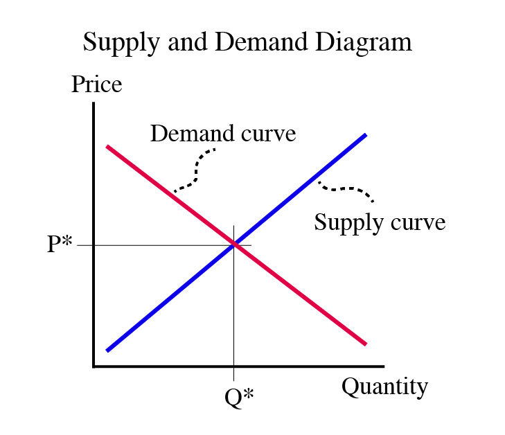
So, looking at Figure 4.1, the demand curve begins on the left, above the supply curve, and as quantity increases as the curves move to the right, they get closer and closer. Then they intersect. This intersection is the point where the utility of consumption of the marginal good is exactly the same as the cost of making it. If we go further to the right, the cost of production is higher than the utility of consumption. This means that for a quantity to the right of the intersection, nobody is willing to pay the full cost of production of the good, with the result that those goods will not be made.
The point where the supply and demand curves intersect is called the Market Equilibrium. An equilibrium is defined as some condition that is not prone to change from minor perturbances. If you drop a marble down the side of a salad bowl, the marble will settle at the bottom and will not move from the bottom unless there is a major disturbance. It is said to be in equilibrium. When a market is in equilibrium, it is not prone to change - it is at a "stable" amount of output at a "stable" price. Equilibrium is where we expect a market to be. Why? If the quantity of goods being produced is lower than the equilibrium quantity (if we are producing at the left of the equilibrium), then there are some people who are willing to pay more than the marginal cost of the good. This means that somebody can make a profit from making more of the good, so we expect production to increase until we hit the equilibrium point. If production is to the right of the equilibrium point, units are being made that nobody will buy, and firms will lose money on them. This incentivizes firms to make less of a good, once again driving the market towards equilibrium.
The equilibrium is not a number, but an ordered pair of numbers: a price and a quantity. We typically use the notation (Q*, P*) to describe an equilibrium. If I ask a question about a market equilibrium, and the answer is only a single number, it will be considered incomplete. An equilibrium consists of an equilibrium price, P*, and the quantity at which that price is observed, Q*. The equilibrium price is sometimes called the "market-clearing" price, meaning that it is the price where the market "clears" all of the goods in it: If the price is below the market clearing price, people will want to buy more, and more will be made. If the price is above the market-clearing price, more will want to be made by producers.
At any given point in time, we expect the market to be in equilibrium. Of course, a market, being the result of human wants, is always changing, and, in this context, you can think of the equilibrium as something that is always shifting, like a set of moving goalposts in a hockey game, but is something that the market is always striving to move towards. The equilibrium is like a magnet, always pulling the market towards it, but always moving, so the market is always chasing. We will talk more about these market dynamics in the next lesson.
Summarizing the supply and demand diagram:
- x-axis: measurement of quantity
- y-axis: measurement of price
- Demand curve: relationship between price and quantity people are willing to buy, derived from marginal utility of consumption
- Supply curve: relationship between price and quantity that firms are willing to sell, derived from marginal cost of production
- Intersection point of supply and demand curves: “market equilibrium”
Perfect Competition
Given all of the assumptions we have made to date, the market that is described above is what we call “perfect competition.” This does not exist in real life, but is a good starting place to study markets.
Perfect competition is based upon four assumptions:
- Nobody has market power. This means that nobody has the ability to change the market equilibrium price based on their own behavior. This means that there must be many buyers and many sellers. We also say “everybody is a price-taker,” which means that they must accept the market price, and they are not “price-setters.”
- Perfect information. This means two things – first, that everybody knows what their own choices are, and also that they know everything about the product.
- Product homogeneity. This means that in a specific market, all products are identical. In real life, no two things are identical, and people make “differentiation” between products. But, for purposes of modeling, we assume that certain groups of products are close enough to being the same.
- Free entry and exit. This means that people only make production and consumption decisions based upon their own free will. They are not forced to buy or sell things they do not want. It also means that people are not negatively affected by other people’s market decisions.
The closest we get to perfect competition is a large stock market like those in New York or London.
A perfectly competitive market gives the greatest possible wealth - we will show just how in the next lesson. Any market that fails to get this full amount is not perfect, and we say that we have a “market failure.” By “failure” we simply mean “not perfect.” All markets are in failure, but some more than others.
Many people wish to correct market failure, and to do this, they usually decide that government must act since no individual has enough power to correct the failures.
However, sometimes in their attempt to fix the problem, the government actually makes things worse (that is, they make the consumer and/or producer surplus even smaller). When this happens, we have what we call “government failure.” We have government failure when a government tries to fix a problem but only makes it worse. Even if the government has good intentions, it usually makes things worse.
Much of the rest of the course will look at deviations from this notion of perfectly competitive markets, that is, violations of one or more of our assumptions of perfect competition, and how these violations play out in real life. We will spend a lot of time looking at market failures, and ways in which we can deal with them, with a focus on how these things affect markets in the energy and resources spheres.
Take Aways
After working through the material on this page and reading the associated textbook content, you should be able to confidently:
- sketch out a supply and demand diagram, and identify the equilibrium;
- define and understand the four assumptions of “perfect competition”:
- nobody has market power
- perfect information
- product homogeneity
- free entry and exit
- understand the concepts of wealth maximization and market failure:
- when is wealth maximized?
- when is a market said to be in failure?
Wealth Created by Markets
Reading Assignment
Read Chapter 9 (Pages 196-215). If you are using an earlier version of the text, read the chapter entitled "Price Takers and the Competitive Process", or, in much earlier versions, "The Firm Under Pure Competition." This is the chapter directly following "Costs and the Supply of Goods."
We have now defined the demand and supply curves and described where they "come from" and how they fit together, giving us a "market equilibrium," which is a combination of a price and quantity that we expect a market to move towards and stay at if there are no external disturbances. If we assume for a moment that we have a stable market that is at equilibrium, we will be able to take a look at how, and by how much, a market system improves wealth in a society. And remember, when I talk about wealth, I am not talking about money, but about the things that improve the quality of our lives. Money is merely a mechanism for interaction that allows us to exchange our labor and investments for goods that we derive utility from.
There are two reasons why we have trade in markets:
- People trying to maximize their utility
- Firms trying to maximize their profits, which increases what they can pay their owners, who can then convert these profits into utility-bearing goods to help maximize owner utility
A reminder: the demand curve is defined by the maximum amount a person is willing to pay for something, which equals the utility gained from consuming goods, which equals the wealth gained. (Wealth ≠ cash). An individual's maximum willingness to pay is sometimes called the "reservation price."
An Aside...
The law of one price. As mentioned above, we are going to assume that the market is in equilibrium. A follow on from this is that the amount of goods sold will equal Q* on the supply and demand diagram and that all of those goods will be priced at the equilibrium price, P*. That is, we are assuming that everybody pays the same price, P*. We call this the "law of one price," and it holds under our assumption of perfect competition. In real life, it is not always true, but as I have mentioned several times, it is a simplifying assumption that is not unreasonable and allows us to use a simple model to develop understanding. As we move through the course, this is one of the assumptions we will relax and look at the effects.
In a perfectly competitive market, we hold that an individual (a consumer, demander, or buyer) will freely enter into a market to exchange money for goods and that a firm (a producer, supplier, or seller) will take that cash in exchange for the good in question. In order for self-interested, non-coerced individuals and firms to enter into such a transaction, it must be in the self-interest of both, and by “in the self-interest,” we mean that each side will gain from the trade. The individual will exchange money for a good that gives him/her more utility than he/she gets from the money, and the firm will gain more money from the sale than it cost to make the good. Remember, people are utility maximizers (happiness maximizers), and firms are profit maximizers.
So, in a (theoretical, perfectly competitive) market, everybody gains something from participating in the market. In the real world, this still holds generally, although not universally, true: most people do not buy things they do not value, and most firms cannot continue to operate while losing money for very long.
The question we wish to ask now is, how much wealth (happiness + profits) is generated by a market? Well, before talking about wealth, let's quickly review the concepts of Consumer Surplus (CS) and Producer Surplus (PS).
A consumer’s net gain of wealth in a trade = maximum amount willing to pay – the purchase price.
(Remember, the maximum willingness to pay is the marginal utility obtained from consuming the good. A rational person will not pay more than the value he gets from the good.) Because we assume the law of one price, all consumers pay the same price, which happens to be the equilibrium price, P*.
Add this up for all buyers, and we have the total wealth created by the market for consumers. This is called Consumer Surplus.
The consumer surplus is the sum of the net wealth gain for each buyer in the market. If a buyer has a willingness to pay (henceforth referred to as WTP) \$10 and the price is \$7, then he has gained \$3 in wealth (\$10 - \$7). If a buyer has a WTP of \$7, he has just broken even (we might say that he is “indifferent” to making this purchase, as he has the same amount of utility whether he makes the trade or not.) If a buyer has a WTP of \$6.50, he would not willingly make the trade, because he is would be exchanging \$7 of money for \$6.50 worth of happiness, and nobody would rationally decrease their amount of happiness (given our assumptions of rational behavior and perfect information).
Note that WTP is the function defined as the demand curve.
So, the consumer surplus (we’ll call this CS to save typing time for me) for the entire market (all buyers added together) is the area between the demand curve and the equilibrium price, to the left of the equilibrium quantity, or the yellow shaded area in the following diagram:

We do not have to worry about what happens to the right of the equilibrium quantity, Q*, because at this point, trades are not made, because the equilibrium price (a constant, and hence, a horizontal line) is above the willingness to pay (above the demand curve) to the right of the equilibrium point.
Now, let’s look at the supply side of the market. Remember our definition of the supply curve:
Supply curve = minimum amount a seller is willing to accept = marginal cost of producing a good.
A producer will not want to sell at below the marginal cost, because this will result in negative net revenue (, so , which equates to a LOSS!). So, any producer in the market will want to sell goods up to the point where price equals marginal cost.
Why? Because this is a profit-maximizing strategy.
Let’s spend a couple of minutes examining why this is. We can assume that we have an UPWARD SLOPING supply curve. In real life, supply curves are usually U-shaped, meaning that the marginal cost of the first few items is very high, then goes down to some minimum point, and then starts to slope upwards (that is, marginal cost will increase with the quantity produced.) Why would MC slope upwards? Because, as you start to add more resources to your production function (remember the previous lesson?), you will have to pay more to attract them away from some other use. There are some special cases where marginal cost is always sloping down – this is something called a natural monopoly that we will talk about later, and is quite common in some parts of the energy industry – but, for the time being, we can assume that near the equilibrium point, the supply curve will be upward sloping, which means that the marginal cost is increasing with increases in Q.
So, if , you are earning an accounting profit of , which is larger than 0. This means you will want to produce more of a good. As you produce more, it gets more expensive, because of the upward slope of the supply curve.
Let’s say we are producing at , with a marginal cost of . Given an equilibrium price P*, then Profit at . Now, we produce at , which means . Profit at , which is smaller than the profit at . The firm will want to keep producing more, and earning a positive but declining profit on each unit, up until we reach the point (call it unit “n”, or ) where . At this point, the accounting profit from marginal unit Qn is exactly zero. Every unit you have produced up to Qn has earned you a positive accounting profit, but now you have hit the point where , so .
As a producer, this is where you want to stop. If you make another unit, the marginal cost will be above the market equilibrium price, and you will make a negative profit (sometimes called a “loss” ) on the next unit. A rational actor will not want to make a loss, so he will prefer to stop at the point where .
This is what we call the “profit-maximizing condition”: profit is maximized when the quantity produced is sufficient to make . Make less than this quantity, and you are leaving money (and profit) on the table. Make more than this quantity, and you will be losing money on some items. In either case, making the quantity will give you the most amount of profit. Hence, the use of the term “profit-maximizing” condition.
I will point out here, again, that we are assuming a “Perfectly Competitive Market,” which is one in which there is perfect information, so every producer will know what his marginal costs are and what the market-clearing price, P*, will be. In real life, this is not true, and producers have to use their best judgment, intelligence, and experience to try to get as close to . But, for the time being, we can assume we have perfect information, just to make understanding of the basic concept a little simpler than real life.
A producer’s net gain of wealth in a trade for a single good = purchase price – minimum willingness to accept. This is the same as “equilibrium price minus marginal cost.”
To get the total profit generated from all goods sold in the market, add the “net gain” up for all goods from sellers, and we have the total wealth created by the market for producers. This is called Producer Surplus (PS).
The minimum willingness to accept (WTA) is defined as the marginal cost curve, which is also called the supply curve.
So, PS is the area between the equilibrium price and the supply curve:

“The sum of consumer surplus and producer surplus is social surplus, also referred to as economic surplus or total surplus.” We also call it the total wealth created by a market.
The qualification about trade only taking place to the left of the equilibrium also applies here. No producer would want to sell to the right of the equilibrium, because the price received will be less than the marginal cost. And, also, the supply curve is above the demand curve, so the price demanded will be above the willingness to pay
The sum of the consumer surplus and the producer surplus is the total wealth created by a market.
Market Equilibrium Example
Example: In a hypothetical market
Demand is given by:
Supply is given by:
- What is the competitive market equilibrium, the consumer surplus and the producer surplus?
- Given the data from Question 1, how much wealth will a consumer make if his willingness to pay is 70? 40? 30?
- Given the data from Question 1, how much wealth will a producer make if his willingness to accept is 70? 40? 30?
Part 1)
At equilibrium, supply equals demand (both quantity and price). So, first, we need to equate the supply and demand functions and find the equilibrium price and quantity .
Then,
At equilibrium
Then, equilibrium quantity will be
By plugging equilibrium quantity ( ) in one of the supply or demand equations (doesn’t matter which one, we should get the same answer), we will find the equilibrium price ( ):
The next step will be calculating the CS and PS at market equilibrium :
And total wealth created by the market

Note for review: Here are the steps in calculating the equlibrium, consumer surplus, and producer surplus:
- P* and Q* can be calculated by solving the supply and demand system of equations for P and Q, which give P* = 40 and Q* = 30
- Consumer surplus is the area of triangle above the P* and below the demand curve (yellow triangle): area = base times height/2
- base of this triangle = Q* = 30
- height = P1 - P*
P1 is the intercept of demand function. So, we can find P1 by plugging Q = 0 into the demand function.
P1 = 100 - 2*0 = 100
Then, height = 100 - 40 = 60 - Consumer Surplus = area of yellow triangle = base * height/2 = (30 * 60)/2 = 900
- Producer surplus, is the area of triangle below the P* and above the supply curve (red triangle): area = base times height/2
- base of the red triangle = Q* = 30
- height of the red triangle = P* - P2
- P2 is the intercept of the supply curve. So, we just need to plug Q = 0 into the supply function to find the P2.
P2 = 10 + 1*0 = 10
So, height of the red triangle = P* - P2 = 40 - 10 = 30 - Producer Surplus = area of red triangle = base * height/2 = (30*30)/2 = 450
Part 2)
: the consumer will make
: the consumer will make
: the consumer will not buy the good because willingness to pay > price
Part 3)
: the producer will not sell the good because willingness to accept < price
: the producer will make
: the producer will make
Practice Exercise
Assume In a hypothetical market demand and supply functions for a good are
Demand:
Supply:
Calculate the competitive market equilibrium, consumer surplus, producer surplus, and total wealth created by the market.
Take Aways
After working through the material on this page and reading the associated textbook content, you should be able to confidently:
- calculate the consumer surplus created by a single trade and by a market;
- calculate the producer surplus created by a single trade and by a market;
- calculate the total wealth created by a single trade and by a market;
- understand why a buyer decides to enter the market (or not);
- understand why a seller decides to enter the market (or not);
- understand why there are no trades to the right of the equilibrium.
Market Dynamics
When we use the world “dynamics,” we simply mean that things change with time, that they do not stay the same. We defined the equilibrium in a market as the point where the supply and demand curves intersect, which is also called the “market clearing” point, where the amount and price of goods that sellers want to sell matches the price and quantity that buyers want to pay. An equilibrium is a “steady state” that things tend towards, and where they will tend to stay unless there is some upsetting force. If you think of a marble in a salad bowl: if you drop the marble from the rim of the bowl, it will move around for a while, but it will settle in the bottom of the bowl, and will not move unless some external force is applied to it – unless it is disturbed.
A market tends towards an equilibrium, but the equilibrium does not stay still. Think about this: the price of a good, and the quantity sold, does not tend to stay the same over time for many goods. For example, in 1998, the average price of gasoline was $1.03/gallon, and about 350 million gallons per day were consumed in the US. By 2007, the price had risen to $2.80, and the consumption had risen to 390 million gallons/day. But in 2009, the average price was $2.35 and consumption had dropped to 378 million gallons/day. Each of these three points represents an equilibrium, and each is quite different.
Figure 4.5 is a plot of the annual average equilibria for gasoline in the United States from 1992 to 2015. The point at the start of the line, near the lower left corner, is the equilibrium for 1992, and the line then travels through the next 24 years.

In this chart, I have population-weighted sales by simply dividing sales by annual average population. You might notice that the path that is followed is pretty predictable for much of the period – the price is fairly stable for several years, from about 1992 to 2002, after which it climbs pretty steadily through 2008. We also see the quantity of sales per person growing quite steadily from 1992 to 2005. Over this period, the average person was consuming more gasoline, but the price was pretty stable. In 2005, volumes were 16% higher than 1992. Then something strange happens – for the years 2006-2012, the path of the equilibrium has “doubled back” on itself, with quantity falling as price tended to rise (if we take out the anomalous bom-bust of 2008 and 2009, prices rose quite steadily from 2005 through 2012. Then, starting in 2013, this trend reversed, and now we are starting to see some modest growth in consumption. We saw a big jump in 2015 as the price dropped a great deal after the oil price crash of Fall 2014. We will talk a little more about “why" in the next section, but I am showing you this path here to illustrate the idea of economic dynamics: how things change with time. Each point on Figure 4.5 represents an equilibrium, an intersection of (not shown) supply and demand curves. But the equilibrium moves with time, with both the equilibrium price and quantity shifting. If each point is an intersection of two lines, clearly one or both of the lines are moving with time. When you look at a standard supply and demand diagram, you are looking at something that is in two dimensions: it has length and width, or price and quantity, and these are both variable, but there is a third variable that we cannot see on the S-D diagram: time. If we had some sort of 3-D paper, there would be not two but three axes intersecting at the origin: price, quantity, and time, and the supply and demand curves would not be lines, but planes that have three dimensions, planes that are wavy and twisty, not flat.
This is a rather long-winded way of saying: things change with time. All things change with time, and markets are no exception.
Results of Changes in the Market
Please read Section 3.3 in the text
In the previous two lessons, we talked about what causes the movements of the supply and demand curves, here we will model the results of these changes. That is, what happens to the equilibrium as market dynamics occur?
Our model of a market consists of two things: a demand curve, and a supply curve. So, when we look at market dynamics, we are looking at a movement of either the demand curve or the supply curve, or, more likely, a movement of both. Let’s take a look at these one at a time first, and then together.
Movements of the Demand Curve
Below, we have a basic, properly-labeled supply and demand diagram. The axes are labeled as price, P (the y-axis), and quantity, Q (the x-axis), the upward-sloping supply curve in red, labeled “S”, the downward-sloping demand curve in blue, labeled “D”, and the equilibrium, at the intersection of the supply and demand curves, labeled “e”, and the equilibrium price and quantity, shown as P* and Q*.

It is important for me to state here: an equilibrium is ALWAYS an ordered pair: (Q*, P*). If I ask a question in a quiz or exam where I ask for an equilibrium, and you give me only a price or a quantity, you will be giving me only half of the answer. Price and quantity.
So, focusing on the demand curve, for the sake of simplicity, we will leave the slope unchanged, and simply look at side-to-side movements. The demand curve can be shifted to the right. This is the same as shifting it upwards, or the same as shifting it diagonally away from the origin. This is called an “outward” shift of the demand curve, as it moves out from the origin. Such a movement is shown in Figure 4.7.
Figure 4.7 shows a movement of the demand curve, from D1 (in light blue) to D2 (in dark blue). Look at what has happened to the equilibrium: it has shifted from (Q*1, P*1) to (Q*2, P*2). Note that P*2 > P*1, and Q*2 > Q*1. In other words, an outward shift of the demand curve results in a larger quantity of goods being sold, and at a higher price. Why? Well, remember that the demand curve is a functional relationship that defines how much people are willing to pay for any given quantity of goods, and this willingness to pay is based on how much happiness people get from consuming one more unit of the goods in question (the marginal utility). When the demand curve shifts outward like this, it means that people are willing to pay more for any given amount of goods. So, given the same upward-sloping supply curve, we can expect more goods to be sold, and at a higher price, because people are willing to pay more, and because they are willing to pay more, producers make more to match their marginal cost with the higher price.
Notice that the equilibrium has moved from e1 to e2. It has moved “along” the supply curve. The demand curve moved outwards, and the equilibrium “slid” along the static supply curve. If you read the popular press, you’ll often see writers talking about “demand for a good increasing.” What they really should say is, “The demand curve has moved outwards, and the equilibrium quantity has increased.”
I will leave it as an exercise for you to figure out what happens when the demand curve moves to the left (which is the same as the demand curve moving downwards, or towards the origin), known as an “inward” movement of the demand curve.
Movements of the Supply Curve
A movement of the demand curve is pretty unambiguous: if the curve moves outwards, equilibrium price and quantity both increase. If the demand curve moves inwards, then equilibrium price and quantity both decrease. Things are a little bit more complicated for movements of the supply curve.
First, let us look at a downward (or rightward) shift of the supply curve while holding the demand curve steady. This is shown in Figure 4.8, with the supply curve shifting from its original position, S1 (in red), to a second position, S2 (in green).
See how the equilibrium has “slid” along the demand curve, from e1 to e2. Now, notice that at e2, quantity has increased (Q*2 > Q*1), but equilibrium price has moved down (P*2 < P*1). This tells us that a movement of the supply curve downwards means that more goods will be sold, and at a lower price. This sounds like a good thing, at least from the consumer’s point of view, but the phrase “supply shifting downwards” might lead a person to think that fewer goods will be made. What is happening? Well, the supply curve is a functional relationship (there’s that phrase again) which describes the marginal cost of producing a given quantity of goods. If the curve shifts down, it means that the cost of producing the nth instance of the good has decreased. Repeating myself: costs have come down. Producers are willing to accept a lower payment for each unit of the good in question because it does not cost as much to produce. A lot of technology goods follow a path like this: when I bought my first personal computer in 1989 it cost me over $3,000, and there were far fewer sold than today. The same goes for my first CD player and first cell phone. As these technologies improved, prices dropped and the volumes sold increased, sometimes dramatically.
So, what happens in the opposite case, an upwards shift of the supply curve? I will leave the diagram to you, but it is not too hard to understand that equilibrium price will increase, and the quantity sold will decrease.
Movements of Both Curves
It is typically true that both supply and demand curves observe shifts over time. Let’s take a look at what happens when both move at the same time. First case, what about an outward shift of the demand curve and downwards shift of the supply curve? This is shown in Figure 4.9.
I have put some arrows on Figure 4.9 to show the downward movement of the supply curve, from S1 to S2, and the upward movement of the demand curve, from D1 to D2. The equilibrium has shifted from point e1 to point e2.
What has happened to equilibrium quantity? It has increased – Q*2 > Q*1. Both movements have led to an increase in Q*. What about equilibrium price? Well, the demand curve movement caused P* to increase, but the supply curve movement caused P* to decrease. One step up, one step down. Which one is bigger? Well, on the diagram, it looks like P*2 is a little bit lower than P*1, but I should make it very clear that this diagram is an illustration, and not to scale. There are no numbers on it. In a real life situation, we will be measuring things and will be able to determine the answer, but here, in the theoretical abstract, we do not know which one is bigger.
We know that Q* increases because the supply curve movement makes the equilibrium move to the right, and then the demand curve movement also makes the equilibrium move to the right. Both changes push quantity in the same direction, so we know that Q* must increase. But P*, we don’t know.
So, to summarize, if D shifts up and S shifts down, then Q* increases and the change in P* is undetermined.
I will leave it up to you to draw diagrams of the other three combinations, but I will give you a shorthand summary of the four results:
Take Aways
After working through the material on this page and reading the associated textbook content, you should be able to confidently:
- understand and describe the changes in market equilibrium caused by an outward movement of the demand curve;
- understand and describe the changes in market equilibrium caused by an inward movement of the demand curve;
- understand and describe the changes in market equilibrium caused by an upward movement of the supply curve;
- understand and describe the changes in market equilibrium caused by an downward movement of the supply curve;
- understand and describe the results of combinations of movements of the supply and demand curves;
- understand the difference between the movement of a curve and the change in equilibrium - that is, the movementOF a curve versus the movement of an equilibrium ALONG a curve.
Market Dynamics Examples
Suppose orange demand function in a small town is given by . Also, supply function is given by . Where P is the price of one pound of orange ($/lb) and Q is the total pounds of orange demanded/supplied in the market (lb). Find the equilibrium price and quantity.
Assume hurricane damages some orange farms this year. Consequently, supply curve is shifted upward. The new supply curve will be . Find the equilibrium price and quantity.
As we can see from the result upward movement of supply shifts the new equilibrium to ( ). The new equilibrium has higher price and lower quantity.
Following the previous example, we found that if demand and supply functions for a local orange market are and , then market equilibrium will be ( )
Now assume, results of a recently published study shows that eating an orange a day will have significant health benefit. And this causes the demand curve to shift outward (to the right). Assume new demand function will be
Find the equilibrium price and quantity
Then, new equilibrium is , which indicates that outward (to the right) shift of demand curve increase equilibrium price and quantity.
And let’s find the equilibrium considering both supply and demands shifts. Assume hurricane damages some orange farms causing the supply curve to shift upward with new supply curve of . Also, the recently published study causes the demand curve to shift outward (to the right) with new demand function of . Find the new equilibrium in the market. What are your expectations on the new equilibrium price and quantity? Higher or lower compared to initial case?
Causes of Market Dynamics I
Reading Assignment
In Chapter 7 ("Consumer Choice and Elasticity"), there is coverage of material concerning complements, substitutes, and income elasticities. You may wish to refer back to this chapter to complement the content here.
In the previous section, we examined what happens to the market equilibrium when the supply and/or demand curves move. Because markets are dynamic things, that is, they are always changing with time, the market equilibrium is always moving. From the previous section, you should understand what happens to a market when the demand and supply curves move up or down (or in or out.) Now we want to consider why these curves move.
It is important to remember that the supply and demand diagram is a static object, but the economy is not static, and things are changing all the time. A supply and demand diagram is only a snapshot of a market at some fixed point in time. We need to understand what causes changes, and what results from these changes.
Causes of Demand Curve Movements
When thinking of things like this, I always like to go back to “first principles.” Or what are sometimes called “fundamentals.” That is, when trying to understand why something happens, try to go back to the underlying root causes. To do that in this instance, we first have to understand what a demand curve is. You should be able to tell me at this point: it is a functional relationship that describes the quantity of goods that consumers in a market will want to purchase at any given price. Digging a bit deeper into the fundamentals, we understand where the demand curve comes from: marginal utility, or how much happiness the consumers obtain from consuming the good.
So, if the demand curve comes from the amount of utility a consumer will get from consuming the good, then the demand curve can only change if the consumers get a different amount of utility from the good in question.
That’s a bit of a mouthful. I’ll try to make it simpler: demand curves change because people change their willingness to pay. They want to buy more or less of the good. The next question then arises: what causes this change in utility?
There are several factors that can cause the demand curve to shift. If the curve shifts upwards (or outwards, away from the origin), then more of a good is demanded by the consumers at a given price. Or, looked at another way, for a fixed quantity, the price will be higher. This means that people derive more utility from a unit of the good. If the reverse happens, and the curve shifts down (or inwards, toward the origin) then less is demanded at a given price, or a lower price will be offered for a certain quantity, and this happens because something has caused the consumer to derive less utility from consumption of the good.
Some Causes of Demand Shifts
Cause #1 – Population
This one is pretty trivial. As we know, a market demand curve is simply an aggregation of every consumer’s individual demand curve. So, it is a matter of arithmetic to understand that if there are more consumers, then there are more individual demand curves to add together, and therefore, the demand curve will be further to the right. There are many examples of this. For example, when Penn State was a much smaller school, in the 1960s and 1970s, there were far fewer apartment complexes in State College. We now have many more apartments than we had in 1970 because there are far more students, and not because students today want to consume more apartments than they did 40 years ago.
Cause #2 – Income
As a person makes more money, their ability to consume more goods increases. The “willingness to pay” increases because the consumer has more money to spend. For this reason, for a lot of goods, as a person makes more money, the individual demand curve shifts to the right. In a community, the wealthier the community, the more the aggregate demand curve moves outwards. This explains why stores that sell luxury goods are usually in well-to-do suburbs, and not poor, inner-city neighborhoods.
To describe this situation, we define something called the “income elasticity of demand.” This is written as follows:
where “I” is the symbol for income
Spelled out, this means “the percent change in the quantity demanded for a given percent change in income.” If your consumption of sushi goes from 2 times a month to 3 when your salary goes up 10%, then your income elasticity of demand for sushi is .
Example, assume demand for economy car falls from 4000 to 3000 units per year if the average real income of the customers decreases from $60,000 to $50,000. Find the income elasticity of demand for the economy car in this town.
Using the income elasticity of demand formula,
The income elasticity can either be positive or negative. If it is positive, then the quantity demanded increases as income increases (a positive number divided by a positive number). Goods that have positive income elasticities are usually referred to as “normal” goods by economists. Luxury cars have positive income elasticities.
It is also possible for a good to have a negative income elasticity. This means that as I increases, Q decreases (a negative number divided by a positive number = a negative number). What does this mean? It means that as a person makes more money, their marginal utility from consuming a certain good declines. I mentioned above that while luxury cars have positive income elasticities, we might say that used cars, or economy cars, have negative elasticities: as people in a society make more money, they are less likely to consume a good. I know that as I have gone through life, my willingness to buy new cars has increased, and my desire to purchase used cars has declined.
Another example might be ramen noodles: students typically do not have a lot of money, so they buy a lot of cheap food, and ramen noodles are about as cheap as it comes. However, when students graduate and get jobs, they can afford to eat better, more satisfying meals, and given that most of us eat a fixed amount of food, this means that the quantity of ramen noodles decreases as income rises. (For the record, I still like a brick of noodles every once in a while, but I do not eat them nearly as much as when I was a student.)
Goods that have negative income elasticities are referred to by economists as “inferior” goods. An inferior good is one that we consume less of as we become wealthier. As we have more money, we can substitute for the inferior good with something that is more expensive, but more enjoyable. We will talk more about substitutes in a minute.
Cause #3 – The Price of Other Goods
The willingness to pay for a good is always relative to the willingness to pay for any and all other goods. The price of some other good can have an effect on our consumption choices.
When we think of how the price of one good can affect the demand curve for another good, we have to define two categories of goods: substitutes and complements.
A substitute is a good that you would consume instead of the good in question. As mentioned above, ramen noodles and steaks can be thought of as substitutes: if you are eating a lot of one, you are likely not eating a lot of the other. Life is full of substitution options: working instead of going to school, taking the bus instead of driving, renting a house instead of buying, taking an expensive vacation versus buying football tickets, going to a movie instead of going to a nightclub, and so on.
A complement is a good that you consume in addition to the good in question, with the condition that without one, you would not consume the other. For example, cars and gasoline (and tires) are all complements. On their own, each of these goods is fairly useless. But use them together, and they suddenly have more value. And, as you consume more of one, you are likely to consume more of another. Think of DVDs and DVD players, or iPods and earbuds, or shoes and shoelaces.
Now, we have to think about how the price of one good can affect the price of another. For this, we define the term “cross-elasticity of demand”. This is defined as follows:
where X and Y are subscripts denoting the two goods in question.
Spelled out, this statement reads: the cross-elasticity of goods X and Y is the percent change in the quantity of good X demanded that corresponds to a percent change in the price of good Y.
Assume demand for chicken is 2000 lbs per day and beef price $3/lb. Holding everything else constant, demand for chicken increases to 3000 lbs per day when beef price increase to $4/lb. Calculate cross-elasticity of demand for chicken.
The cross-elasticity can be either positive or negative, and the sign will tell us if goods are substitutes or complements. In the previous example cross-elasticity of chicken and beef is positive. So, we can say they are substitutes.
Let’s think of two common substitutes: chicken and beef. It is not hard to understand that if the price of beef goes up while the price of chicken stays the same, then people will tend to substitute chicken for beef. So, as the price of beef increases, the quantity of chicken demanded increases. The cross-elasticity in this case is a positive number divided by a positive number (or a negative divided by a negative), which gives us a positive number. Therefore, substitute goods have a positive cross-elasticity.
Now, let us think about complements. In the 1980s, CD players came on to the market. At first, CD players were very expensive, and very few people had them. Correspondingly, there were fewer music CDs sold. Over time, the price of CD players came down, and as a result, the quantity of CDs sold increased dramatically (even though the price did not change much for many years). It is easy to see that CD players and CDs are complements: one of the two is of little use without the other. So, when we look at our formula for the cross-elasticity, a decrease in the price of CD players led to an increase in the quantity of CDs demanded. A positive number ( ) is divided by a negative number ( ). Thus, the cross-elasticity is negative.
This leads to the definition of a handy rule: if the cross-elasticity of two goods can be shown to have a consistently positive value, then the goods are substitutes. If the cross-elasticity is shown to be consistently negative, the goods are complements. If the cross elasticity is either zero, or inconsistent, then it is likely that the goods are neither complements nor substitutes, but unrelated. Obviously, in our complicated economy, everything is related to everything else - the price of jet planes in Europe probably has some effect on the price of corn in Illinois, but the effect of one on the other is so dispersed as to be unobservable in any meaningful manner.
Causes of Market Dynamics II
Cause #4 – Expectations
This is similar to income, but instead refers to future changes that a buyer expects to happen in the near future. For example, if you expect gasoline to be more expensive next week, you are more likely to fill up this week. This will cause the equilibrium for gasoline to shift today.
Cause #5 – Taste (or Fashion)
Some things, such as music styles, car models, clothing or house furnishings change in style over time. As such, desires for certain styles can change. What is fashionable, and popular one day may be out-of-date and unwanted the next. For example, why is it that skinny ties or Britney Spears CDs sell millions in one year, but are not popular a couple of years later? This is a point where economics starts to approach psychology, which is an area where I have little expertise. At this point, we need simply be content with the fact that at different points in time, people will want to buy different quantities of things for reasons that do not have any direct economic causes.
Cause #6 – Information
Going back to fundamentals, the demand for a good is based upon the utility, or happiness, one gets from consuming it. Sometimes, new information comes onto the market that leads to a change in the happiness that someone derives from consuming a good. The most obvious example of this has to do with health information. We often learn that consumption of a good may have beneficial or detrimental effects on one’s health. A few years ago, the “Atkins” diet was popular, in which it was believed that people could lose weight by eating a diet that was high in proteins and low in carbohydrates. A lot of people adopted this diet, so much so that many bakeries went out of business because bread sales declined a great deal. A little while later, some detrimental health effects of the Atkins diet were publicized, and this caused some people to abandon this diet. Fewer people smoke today than in the past, because we have better information about the long-term effects of smoking on health.
Health information is not the only form of information that can move demand curves. For example, when some people publicized what they felt were poor working conditions in clothing factories in Asia, a number of people in the US decided against purchasing goods made in those factories. In other cases, people fall out of favor. There are probably not too many Brett Favre football jerseys being sold in Green Bay these days, even though he was a hero in that city for many years. Deciding to play for a rival team in Minnesota greatly reduced the demand for clothing with his name and picture on it in Green Bay.
Causes of Movements of the Supply Curve
Unlike changes in demand, changes in supply are usually simpler to explain. A downward shift of the supply curve, which means that more goods are supplied at the same price, usually results from a lowering of the cost of production. This cost reduction could be because of a new, more efficient technology, or could be because of lowered taxes, or cheaper labor costs.
An upward shift of the supply curve (less being offered at the same price) is usually the result of some disturbance in the market. The most common example is when crops are damaged by weather conditions: hurricanes, unexpected cold, not enough rain, and so on. If prices for materials or labor of energy, any of the things that go into making a good, have increased in price, then the supply curve shifts upwards. If a tax on a good is increased, then the supply curve will shift upwards, as a tax is a cost that has to be paid on the good, not to the seller of the good or to the sellers of the factors of production, but to government. We will talk more about the incidence and effects of taxes later in the course.
Sample Question
Let us suppose that the following two events happen simultaneously:
- The Food and Drug Administration releases a report showing that drinking orange juice causes bald men to grow hair.
- A giant freeze destroys the orange crop in Florida, meaning that we have to import all of our oranges from Brazil for a year.
What do you expect to happen to the equilibrium price and quantity of orange juice?
Answer
The first statement will likely cause many bald men to start drinking more orange juice. This will cause an outward shift of the demand curve.
The second statement means that oranges will likely be more expensive to produce, which corresponding to an upward shift of the supply curve.
The demand curve movement will increase the equilibrium price and quantity. The supply curve movement will increase the equilibrium price, but reduce the equilibrium quantity.
Therefore, the net result will be an increase in the price of orange juice (both curve movements cause price to increase), but the change in quantity sold is unknown from the information at hand. One movement increases quantity sold, the other decreases it. Without measurement, we do not know which effect will dominate the other.
Conclusion
When prices change, they change because either the supply curve or demand curve (or both) has moved. Whenever a price changes, to understand why we want to figure out which of the underlying curves has moved, and why. After working through this lesson, you should be able to explain what happens when supply and demand curves move, and what some of the common causes of such movements are.
Take Aways
After working through the material on this page and reading the associated textbook content, you should be able to confidently:
- explain the basic causes of the movements of the demand curve;
- changes in tastes
- the prices of other goods
- changes in income
- new information
- expectations
- population changes
- understand the concepts of complementary and substitute goods;
- explain how cross-elasticity is linked to the definition of substitutes and complements
- understand what the sign of the cross-elasticity implies
- understand the concepts of normal and inferior goods;
- explain how income-elasticity is linked to the definition of substitutes and complements
- understand what the sign of the income elasticity implies
- explain the basic causes of upwards and downwards shifts of the supply curve;
- understand that the supply curve is strongly related to the cost of producing goods.
Summary and Final Tasks
In this lesson, we studied the notions of wealth creation in markets - how both buyers and sellers can be made "better off" (increase their utility or profits) by participating in markets. We then addressed the concept that a market is a dynamic thing - it is constantly changing with time. Since we model a market by using two things: a demand curve and a supply curve - we are able to examine all changes in a market by movements of the supply and demand curves.
We looked at what happens to markets when supply and demand curves move. We then examined the root causes of movements of the supply and demand curves.
Have you completed everything?
You have reached the end of Lesson 4! Double check the list of requirements on the first page of this lesson to make sure you have completed all of the activities listed there.
Tell us about it!
If you have anything you'd like to comment on or add to the lesson materials, feel free to post your thoughts in the discussion forum in Canvas. For example, if there was a point that you had trouble understanding, ask about it.
Lesson 5 - Market Power
Lesson 5 Overview
In the previous three lessons, we learned the fundamentals of supply and demand in the framework of perfect competition. In this lesson, we will begin to relax some of the assumptions of perfect competition, and see what happens in markets when some participants have what we call "market power." This will help explain what happens in some energy markets.
What will we learn?
By the end of this lesson, you should be able to:
- list and describe the assumptions that define "perfect competition;"
- understand and explain what is meant by the phrase "market power;"
- define "monopoly" and understand monopolistic behavior;
- show the differences between competitive and monopolistic equilibria;
- explain the effects of other types of market power;
- describe how we can measure market power;
- describe what a cartel is, and how it manages prices.
What is due for Lesson 5?
This lesson will take us one week to complete. Please refer to Canvas for specific time frames and due dates. There are a number of required activities in this lesson. The chart below provides an overview of those activities that must be submitted for this lesson. For assignment details, refer to the lesson page noted.
| Requirements | Submitting Your Work |
|---|---|
| Reading: (see lesson pages for exact assignments) | Not submitted |
Perfectly Competitive Markets
Reading Assignment
From Gwartney et al. please review the Chapter 9, "Price Takers and the Competitive Process."
From Greenlaw et al. please review the chapter 8,"Perfect Competition".
As mentioned earlier in the course, the kind of market we have been examining in the past few lessons, the simplified supply-and-demand diagram, and the underlying assumptions about rational utility maximization, supply being defined by marginal cost, and the law of one price, are all part of what we call "perfect competition.” As I have said, this is an idealization. It does not exist in real life, but is a good starting place to study markets.
When we talk about "perfect," we mean that this form of market gives the best possible outcome with respect to "aggregate wealth," which is just consumer surplus and producer surplus added together. There are many ways in which markets can generate less than optimal quantities of wealth - cost can be too high, people might not know certain information, costs can be borne by others, people can manipulate markets to charge a price that is either higher or lower than the market equilibrium, and so on. In real life, it is safe to say that there is no such thing as a perfect market; that, in every case, there is a distortion of some sort that adversely affects prices, quantities, or wealth. At this point, we will go over, once again, the four things that we assume for perfectly competitive markets to exist, and over the next few weeks we will look at what happens if one or more of these assumptions is violated.
If a market produces less than the optimal (maximum) amount of wealth, then we say we have "market failure." This sounds a bit extreme - anything less than perfection is called "failure." It's a good thing college isn't like this - anything less than 100% is a fail. So, we have to consider that there are "degrees" of market failure, just like there are degrees of success in a course. Getting 90% in a class is better than getting 40%. My car having a broken clock is a lot better than having a broken transmission, even though both represent some degree of "failure." So, when we think about market failure, we have to understand when it is serious, and thus needs some fixing, or when it is not, and trying to fix it will only make things worse.
So, let's go through the four assumptions of perfect competition, and their meanings.
Nobody Has Market Power
This means that nobody has the ability to change the market equilibrium price based on their own behavior. This means that there must be many buyers and many sellers. We also say “everybody is a price-taker,” which means that they must accept the market price, and they are not “price-setters.” When we say that "nobody has the ability to affect price based upon their own decisions," then each market entrant must be small compared to the size of the market in general, such that one consumer choosing to consume or not does not "meaningfully" change the market price based upon his/her decisions. As we have seen, a market is an aggregation of individual desires and actions, and, in theory, a change in the consumption habits of some part of the market will be reflected in the form of the market as a whole. In theory, me choosing to buy peaches instead of oranges at the grocery store will affect the markets for both peaches and oranges. However, since I am only one of several hundred people that buy fruit daily in that store, my consumption choices will have a very small, almost imperceptible, effect on the price of either good.
This is sometimes called "atomistic" competition, referencing the idea of elementary particles from physics. We, and everything around us, are composed of atomic particles, but the adding or changing of a few particles does not change us in a "meaningful" manner. So, to reiterate: "nobody has market power" means that everybody is a price-taker, not a price setter, and it means that there are so many individual buyers and sellers that the actions of one or a few will not meaningfully change the market equilibrium.
Perfect Information
This means two things – first, that everybody knows what their own choices are, and also that they know everything about the product. When we say "know your own choices," we mean that you are capable of knowing what amount of marginal utility you will receive from consuming a product, and you will also know the amount of marginal utility you will obtain from consuming every possible other consumption choice. This means that when you consume something, you will definitely be spending money on the thing that maximizes your utility.
Clearly, this is an unreasonable assumption. We do not spend every waking minute calculating the marginal utility of consumption. We can't, for several reasons. Firstly, the universe of choices is too large to consider every option. Secondly, some of your consumption choices take place in the future (that is, should I spend now or save my money and spend later?) We do not know the future. We do not know how much money we will have in the future; we do not know how our tastes and needs will change in the future. The final point is, it can be difficult to measure "happiness" from a consumption choice. Smoking a cigarette might make somebody happy today but very unhappy in a few years if he gets lung cancer. How can we calculate and assign values to such things? We can't.
A great deal of work on the frontiers of economics (the part that intersects with psychology) is about trying to figure out how and why we make choices. This is not something we can address here. That is fine - we are interested in studying what kind of market outcomes we have from the results of those choices, and trying to come up with some general observations, with a bit of predictive power, about how people behave in markets. If you are interested in this area of study, you might want to take a look at a field called "behavioral economics," which concerns itself with examining why people make choices that seem, on the surface, to be against their own best interests. Many people who study in this area claim that their findings undermine the axiomatic assumption about rational utility maximization, but I prefer to think that most "irrational" behavior can be tied back to imperfect information.
A second component of information is a bit simpler to understand: information about a product. That is, when we buy something, do we understand what we are getting? If I buy a Rolex watch, I expect something made in the Rolex factory in Switzerland, not something made in China. If I buy the Chinese Rolex, thinking that it is a Swiss one, I do not have perfect information. On a more mundane level, with reference to the law of one price, am I able to get the best price? For example, I recently moved to a new city. I like to send my shirts out to be laundered, mostly because I am very bad at ironing shirts. There are several dry cleaners near where I live, so how do I know that I am getting the best price? Well, I have to invest some time and effort into discovering the prices at each of these places. What if there is a place that I missed? What if a place does not have an informative website, or will not tell me their prices over the phone? These are all types of information market failure, some more serious than others.
Speaking of the supply side of the market, the most important type of information is cost information. This may seem like a simple idea - a firm can figure out what it's spending money on - but sometimes it can be very difficult figuring out the marginal cost - the cost of producing one more item. It can also be very difficult to make production function and investment choices: should a firm expand, or buy more machinery, or hire more staff? This can be difficult to assess because the alternate states of the world that they entail in the future are unknown.
Product Homogeneity
This means that in a specific market, all products are identical. In real life, no two things are identical, and people make “differentiation” between products. But, for purposes of modeling, we assume that certain groups of products are close enough to being the same.
In many industries, firms go to great efforts to differentiate their products from others. Some of the best examples are soft drinks, hair care products, and cars. The primary tool for product differentiation is advertising. The reason that firms do this is to be able to charge higher prices. For example, a four door car with a four cylinder engine may be an undifferentiated product, but if it is a four-door, four-cylinder car with a badge on the front that says "Toyota" or "Ford," then it is a differentiated product, and each of those manufacturers will try to charge more by convincing you that the name on the front has some extra value. This is another case where modeling consumer choice becomes a bit more difficult.
Free Entry and Exit
This means that people only make production and consumption decision based upon their own free will. They are not forced to buy or sell things they do not want. It also means that people are not negatively affected by other people’s market decisions. In situations where a private economic transaction negatively affects a person who is not a willing participant in that economic transaction, we have something called an "externality." This is a very important type of market failure, and one we will study at length in the next few weeks. The most important externality we will study is pollution, which is a major issue in energy markets and is the basis for the field of environmental economics.
Another aspect of free entry is that competitors can not put up "barriers to entry".
As mentioned above, there is no such thing as a perfectly competitive market. Probably the closest we get to perfect competition is a large stock market like those in New York or London. Think about why: there are usually many buyers and sellers, there is a lot of information about the value of a company behind the stock, a share of a company is identical to any other share of that company, and there are no externalities.
Reiteration
A perfectly competitive market gives the greatest possible wealth – the sum of consumer and producer surplus. Any market that fails to get this full amount is not perfect, and we say that we have a “market failure.” By “failure” we simply mean “not perfect.” All markets are in failure, but some more than others.
Many people wish to correct market failure, and to do this, they usually decide that government must act, since no individual has enough power to correct the failures.
However, sometimes, in their attempt to fix the problem, government actually makes things worse (that is, they make the consumer and/or producer surplus even smaller). When this happens we have what we call “government failure.” We have government failure when a government tries to fix a problem, but only makes it worse. Even if government has good intentions, it usually makes things worse.
In the next few sessions, we will talk about market failure and then move on to studying government failure.
Market Power and Monopoly
Reading Assignment
For this section, please read Chapter 11: "Price Searcher Markets with High Entry Barriers." from Gwartney et al.
From Greenlaw et al. chapter 9,"Monopoly".
Our first assumption is that of market power, which states that everybody is a price taker, or that there are many buyers and sellers in a market. In this case, the equilibrium price in a market is defined by so many different transactions that anybody who wishes to buy or sell in this market has to do so at the market equilibrium price, and they are not able to move the equilibrium price with their own actions. Hence, you have to "take" whatever the price is. If you are able to move the equilibrium price with your own choices, then you can be referred to as a "price-setter." In reality, in many situations, somebody in the market has some power to change prices through their individual actions. These include:
- Monopoly: only 1 seller.
- Duopoly: 2 sellers.
- Oligopoly: a few sellers.
- Monopsony: only 1 buyer.
Monopoly
This is the most extreme, but not the most common, example of market power. A monopoly is a market with only one seller. A monopolist is free to set prices or production quantities, but not both because he faces a downward-sloping demand curve. He cannot have a high price and a high quantity of sales – if he has a high price, people will buy less.
There are three ways that a monopoly can exist and/or persist:
- All of some resource is owned by some firm (e.g., deBeers and diamonds).
- The government allows a monopoly to exist (not common in the US, but in many countries things like airlines or railways are government-designated monopolies).
- A Natural Monopoly exists (e.g., your local power company). We will talk more about natural monopolies a bit later in the course.
At this point, you might think about some markets that have a dominant market share held by a single firm, such as Microsoft in the market for spreadsheet software. These are not monopolies, in that firms in these markets do have competitors, and consumers do have choices. If a firm obtains an inordinate market share due to offering a product that many people want to buy, we do not have a monopoly. Firms in a case such as this may have a lot of market power, and may face a lot of scrutiny from the government, but they are not technically monopolies.
Why is a monopoly bad?
Monopolies are typically assumed to be undesirable market structures. They are undesirable, or "bad," because in this case "bad” means less than the most possible total wealth – the sum of the producer and consumer surpluses. A market in which there is a monopoly will generate less wealth for a society than a competitive market would.
A monopoly leads to the following:
- A lower quantity of goods produced and consumed than in a competitive market.
- A higher price than the equilibrium price in a competitive market.
- A higher profit for the firm. In a monopoly, a firm will typically make greater than zero economic profit (remember that term?).
In a competitive market, it is the act of competition that drives prices towards the equilibrium price and quantity at which the marginal firm makes zero economic profits - they are earning just enough money to cover their costs of production and to pay their owners a return that is sufficient to cover their risks. If firms in an industry are making positive economic profits, then other firms have an incentive to enter the market to try and deliver these positive profits to their owners. Generally, this extra market entry is enough to increase production and decrease equilibrium price to the point where zero economic profits are seen. In a monopoly, these competitive pressures are absent. A firm is able to earn positive economic profits, and because they are a monopoly, other firms are unable to enter their market and drive down price.
This leads to an increase in the size of the producer surplus and a decrease in the size of the consumer surplus. As a disinterested economist, we might say "who cares?" especially if we are generating wealth. That is, should we care who gets the wealth, as long as wealth is being generated? That would be a "normative" statement. However, since we are concerned with maximizing the aggregate wealth of a society, we can ask the positive question "does a monopoly decrease total wealth generated?" If it does, then we have the definition of a market failure.
It is quite easy to answer this question with a supply and demand diagram. But first, consider how a monopoly works. We may have a single seller, and this seller may be able to choose his price, but he cannot control the demand curve. Remember, the demand curve is defined by the marginal utility of consumption, a measure of how much happiness the consumers get from consuming. So, the monopolist faces a demand curve he or she cannot change. So what a monopolist can do is choose just where the supply curve intersects the demand curve. He can choose any combination of price or quantity that exists along the demand curve. If he picks a high quantity, then he chooses a low price, or vice-versa. He cannot have a high price and high quantity. When I say "high" here, I am speaking in relationship to the competitive market equilibrium.
So, a monopoly producer will typically restrict output to some quantity below the market equilibrium. This is illustrated on the following supply and demand diagram, where refers to the quantity produced by the monopolist. To find out what price we see in this market, draw the line up from until it intersects the demand curve. This gives us the monopoly price, . These contrast to the "free-market" equilibrium, which I label as and in this diagram.
As you can see, since < , then has to be greater than , because the demand curve is downward-sloping.

In a competitive market, wealth is the sum of the red, yellow, and blue areas. In the monopoly market, it is just the sum of the yellow and red areas. The blue area is wealth that is lost to society. This area is the Deadweight Loss. This labeled as "DWL" in Figure 5.1. This is the cost to a society of allowing a monopoly to operate. So, in a monopoly, the producer makes more, the consumer makes less, and the society, added together, is poorer as a result.
This is called a Social Cost: a cost to the total society.
Example
Demand is given by , Supply is given by . If the monopolist sets , what is the dead-weight loss?
Answer:
In order to find the dead-weight loss, we need to calculate the area of triangle bounded to the equilibrium point and monopolistic quantity (Qm).
Competitive market equilibrium is defined by the intersection of supply and demand, so if and . Then,
so,
.
Thus, .
If we substitute with 90 in either the supply or demand curve, then we get .
So, the equilibrium price and quantity .
The consumer surplus will be 720 x 90 x 0.5 = 32,400, and the producer surplus will be 8,100. (Why?) The total wealth generated by this market will be 40,500.
Now, how much wealth is lost if the producer can restrict output to 50?
Well, firstly, the monopoly price will be set by the demand curve, which is given by , which gives us 900 - 8*50 = 500. So, the monopoly equilibrium will be . The dead-weight loss is the triangle between the demand and supply curves and the vertical line Q = 50. The area of this triangle is 400 x 40 x 0.5 = 8,000. So, the dead-weight loss is 8,000, and the total wealth generated by this market is only 32,500. This is about 20% reduction in total aggregate wealth generated by the market. Note that consumer surplus has been reduced to 10,000 from 32,400, and producer surplus has been increased to 22,500 from 8,100. So, in this market, the producers earn 14,400 units more wealth, the consumers earn 22,400 units less, and the market generates 8,000 fewer units of wealth.
Where did this wealth go? It is the lost potential wealth from trades that would take place between Q = 50 and Q = 90. In this market, there are consumers whose willingness to pay is above the market equilibrium price, but they are unable to buy because the monopolist will not sell to them. Now, why on earth would a monopolist not want to sell something? Well, let's see why.
Profit Maximizing in a Monopoly
The goal of a firm is to maximize profits. So, if a firm is free to set whatever price (or quantity) they want, which level will maximize profits?
Profit (producer surplus) is the area below the equilibrium price and above the supply curve. The supply curve is the same thing as the Marginal Cost curve for the firm.

(Note: in Figure 5.2, I use and to represent “monopoly equilibrium quantity” and “monopoly equilibrium price.")
At which value of is the producer surplus (the profit, the red area) the largest?
Answer: it is maximized when supply = MC = MR (Marginal Revenue).
What is marginal revenue? Well, it is the amount of money a firm takes in from selling one more unit of the good. If the price is constant, then MR = price - selling one more unit means we collect one more times the price. But, in this case, since the monopolist faces a downward sloping demand curve, each additional unit he sells will have a lower price, and he will sell every unit at that lower price. As an example, using the demand curve in the previous numerical example, if the monopolist sets , then he sells 50 units at a price of 500, and has total revenue of 500 x 50 = 25,000. If he makes one more unit, he sells 51 units at a price of 492 (price is derived from the demand curve, 900-8*51=492), for a revenue of 25,095. His marginal revenue from making one more unit is 95, even though the price is 492.
So, we need to plot the marginal revenue curve.
It turns out that the marginal revenue curve is a line that has the same y-intercept as the demand curve, but has a slope that is twice as steep. So, for example, if our demand curve is given as , then 100 is the intercept and -1 is the slope (remember the equation of a line; . In our case, , which is another way of writing .
So, the marginal revenue curve has the same intercept, 100, but is twice as steep, with a slope of -2.
This is written as:
An Aside...
Here is a small aside, which is not obligatory and not something you will be quizzed on. If you know calculus, you will be able to understand the following calculus-based explanation of why the monopolist sets his quantity to be that where MR = MC, and how we derive .
A monopolist wants to maximize profit, and profit = total revenue - total costs.
We can write this as . In calculus, to find a maximum, we take the first derivative and set it to zero:
Profit is maximized when
= marginal revenue and = marginal cost
So, is the same as , which is the same as MR = MC.
To find MR: .
If the demand curve is given by then
So,
So, the MR curve has the same intercept as the demand curve, but its slope is exactly double that of the demand curve.
Generally, if a Demand curve is given as , then .

In Figure 5.3, the MR curve is shown in blue. To find the profit maximizing point, set to the amount where the MR and MC curves intersect. These will be sold at price . Any other quantity will give a smaller profit (the red area on the graph).
So, it is important to remember two things:
- The marginal revenue (MR) is a line with the same intercept as the demand curve, but with a slope twice as steep; and
- When , profit is maximized.
We say that in a monopoly, profit is maximized when , just like in a competitive market, when MR = Price = MC. You will remember that in a competitive market, the demand curve is flat. Its slope is zero. So, the derivative of this curve, which is the MR curve, also has a slope of zero (two times zero = zero). So the result that P(max) occurs when MR = MC is true not just in a monopoly, but all markets.
Example
The demand curve is given as: .
The supply curve is given as: .
- What is the profit-maximizing (monopoly) equilibrium?
- Find the Consumer Surplus and Producer Surplus
- What is the dead-weight loss?
Answers:
-
In order to answer this question, first, we need to find the monopoly equilibrium. To do so, first, we have to solve the MR = MC for the Q. MC is the supply function, and we learned that if demand curve is given as , then
So, MR equation will be .And will be set by the demand curve:
-
Consumer surplus equals the area of the under the demand curve and monopoly price , horizontal line.
Coordinates of three corners of this triangle will be:
Top left: (0, demand curve intercept) = (0, 140)
Bottom left:
Right corner:Producer surplus equals the area of the under the monopoly price and above the supply curve (red area), which equals the area of the trapezoid.
Coordinates of four corners of this trapezoid are:
Top left: (0, Pm) = (0, 100)
Bottom left: (0, supply curve intercept) = (0, 20)
Top right:
Bottom right:Note that coordinate of bottom right corner of the trapezoid (MR and supply curve intersection) can be found by plugging the Qm in the supply curve,
And the area of the trapezoid will be:
-
The dead-weight loss is the triangle between the demand and supply curves (competitive market equilibrium) and the vertical line Qm. So, first, we need to find the competitive market equilibrium:
Demand curve: .
Supply curve: .At the competitive market equilibrium: demand = supply
140 – 2Q = 20 + 2Q
Q* = 30
P* = 140 – 2*30 = 80Coordinates of three corners of this triangle will be:
Top left: , which is (20, 100)
Bottom left: = (20, 60)
Right: = (30, 80)Now that we have the coordinates of three corners, we should be able to find the area of the triangle as:
Dead-weight loss
Note that dead-weight loss can also be calculated by deducting the monopoly market total wealth (CS + PS) from competitive market total wealth.
Your turn!
Practice Exercise
Assume In a hypothetical market demand and supply functions for a good are
Demand:
Supply:
- Calculate the competitive market equilibrium, consumer surplus, producer surplus, and total wealth created by the market.
- Calculate the monopoly Price and quantity, consumer surplus, producer surplus, and total wealth.
- Caclulate the dead-weight loss of the monopoly.
Calculate the dead-weight loss using this method and compare your answer with what we calculated. You should have similar results.
Try and work it through and see if you can get these answers.
Take Aways
After this lesson and the associated readings, you should be able to:
- define and understand the meaning of “market power;”
- know the names of markets with:
- one seller,
- two sellers,
- a few sellers,
- one buyer;
- understand why a monopolist can set price or quantity, but not both;
- describe the three ways a monopoly can come into existence;
- explain the effects of a monopoly on price and quantity compared to a free market;
- understand what happens to consumer and producer surplus in a monopoly;
- understand the concept of a “dead-weight loss” and a “social cost;”
- understand and apply the rule for profit maximization in a monopoly;
- find the marginal revenue curve:
- the intercept of the marginal revenue curve,
- the slope of the marginal revenue curve;
- find the monopoly equilibrium and compare it to the competitive equilibrium.
Other Forms of Market Power
Single buyer = Monopsony
In this case, a buyer has market power and tries to maximize the consumer surplus, not the producer surplus. We essentially have a monopoly in reverse, and consumer surplus is maximized by the consumer's choice of quantity purchased. Instead of looking at the producer's marginal revenue function to define the monopoly quantity and price, we instead look at the consumer's "marginal expenditure," the amount of money he has to spend to obtain one more unit of a good, which changes with his purchase decision. Once again, we have a quantity that is less than the free-market equilibrium, but in this case a price that is lower than the free market equilibrium. This is described in the following diagram:

As you can see in Figure 5.4, the “Marginal Expenditure” line has the same intercept as the marginal cost line, but double the slope.
Monopoly-Monopsony
It is possible to have a situation where there is only one buyer and one seller. In this case, the quantity sold and the price will be a function of the negotiation between the trading partners.
Duopoly
This is the case where we have two sellers. Without getting into the mathematical details, we discover that the price is lower than the monopoly price, but higher than the competitive price. The quantity is also between the two. The best outcome for the two firms would be to share the monopoly profits between them; but each side has an incentive to cheat, which results in a different equilibrium. Incentives to cheat in a collusive environment are described in Chapter 11 of the text.
Oligopoly
In this case, we are adding a few more sellers. As we add more sellers, the equilibrium moves along the demand curve towards the competitive equilibrium, as in the following diagram:

The obvious conclusion is that the more firms in a market, the closer we get to the competitive (wealth-maximizing) solution. This is why governments generally try to stop monopolies and break market power.
Take Aways
After this lesson and the associated readings, you should be able to:
- define an equilibrium in a monopsony;
- compare a duopoly equilibrium to monopoly and competitive equilibria;
- understand how an oligopoly equilibrium compares to monopoly and competitive equilibria;
- understand what happens to the equilibrium as we add more firms.
Price Discrimination
Reading Assignment
Please read the section on Price Discrimination in Chapter 10, "Price-Searcher Markets with Low Entry Barriers." In the most recent version of the book, this is on pages 198-200.
Because we have a deadweight loss in a monopoly, some social wealth is not collected. This means that a society is poorer, in total, because of the existence of a monopoly. But it is possible for a producer to capture some of this lost wealth. This can be done by using price discrimination. Price discrimination refers to charging different prices to different customers. In a perfectly competitive market, this is not possible, because there are many firms competing for the price; but it is possible in a monopoly, because people have no other place to buy.
If the seller is able to discover just what price the buyer is willing to pay (what the buyer’s Reservation Price is), and offer a price incrementally below the reservation price, then the seller is capturing basically all of the total surplus.
There are three general ways in which price discrimination can occur:
- First degree (or perfect) price discrimination refers to charging a different price to every consumer. This is not very possible in real life.
- Second degree price discrimination refers to charging different amounts for different sized purchases. If a car rental company buys 300 cars from a dealer, they will get a better price than if I go and try to buy 1 car. This is known as bulk pricing.
- Third degree price discrimination refers to breaking up the market into different groups who have different demand curves and maximizing profit in each different market sub-group. For example, a restaurant might have a special children’s menu, with small portions at lower prices. Adults would not want to buy these small portions, but forcing adults to buy adult portions for children might make the customers decide to stay home.
Example
The Philadelphia Zoo discovers that they have two groups of customers with two different demand curves. Locals have demand , and tourists have demand . What is the profit maximizing set of prices? (The marginal cost of visitors is zero.)
Solution:
In this case, we have two separate demand curves, and as a monopolist we wish to maximize profit by charging each separate part of the market a separate, monopolistic price.
For locals, demand is given as , so .
- Since , then setting gives us , or .
- Entering into the demand curve gives us
For tourists, demand is given as , so .
- Since , then setting gives us , or .
- Entering into the demand curve gives us
So, the answer is, if it wishes to maximize profits, the zoo should charge locals \$20 for admission, and \$25 to tourists. Of course, in this case, the trick involves being able to effectively separate locals and tourists.
Take Aways
After this lesson and the associated readings, you should be able to:
- explain what first-degree price discrimination is;
- explain what second-degree price discrimination is;
- explain what third-degree price discrimination is.
Measuring Market Power
Herfindahl - Hirschman Index (HHI)
Governments are interested in controlling market power, and to do this they need a way of measuring it. The most common tool is called the Herfindahl - Hirschman Index (HHI)
This is the sum of the squares of each firm’s market share, expressed in percentage terms:
where Si is the market share of firm i in percentage. Market share can be calculated as firm's sale divided by total market sale.
So, if we have one firm in an industry, the HHI will be 10,000, and if we have an infinite number of tiny firms, it will approach zero.
Example
Say we have an industry with four firms. They have market shares of 40%, 30%, 20% and 10% respectively. What is the HHI?
HHI =
Now, what happens if the largest firm buys out the third largest firm?
Now, we have three firms with the following market shares: 60%, 30% and 10%.
So, the HHI . The concentration has increased by over 50%.
- If the HHI is less than 1000, a market is generally considered to be not concentrated.
- If the HHI is between 1000 and 1800, a market is thought to be “moderately concentrated.”
- If the HHI is above 1,800, the industry is considered to be highly concentrated.
In the third case, governments will often act to reduce concentration. This is called an “anti-trust” action.
Cartels
A cartel is a form of market power in which suppliers collude with each other to manipulate supply. The most famous cartel in the world is OPEC, the Organization of Petroleum Exporting Countries. It turns out that crude oil is found in many countries in the world. In fact, there are probably oil wells in pretty much every country in the world. But there are a few countries that have large supplies of oil that is relatively cheap to produce.
The history of the international oil industry is convoluted and full of lots of stories about power, colonialism, and nationalism. The oil in many parts of the world was controlled for about half a century by a group of American and European companies called the "Seven Sisters." The countries in which the oil was found resented this control, as they believed that the price was being kept artificially low to benefit the consuming, and not producing countries. Several of these countries banded together to take control of their own resources and formed the organization we know as OPEC.
As I mentioned, there is a lot of fascinating history in the oil industry and OPEC. If you have more interest, I suggest you look at the Wikipedia page for OPEC for a quick overview, and if you are interested in investing a little more time, I recommend reading the book "The Prize" by Daniel Yergin. However, this is an economics course, and I want to focus on the economics of cartels.
OPEC is able to act somewhat like a monopolist, even though the oil industry is not a monopoly. OPEC countries produce about 30% of the world's oil. However, they produce a lot of low cost oil, so they are able to effectively control the supply curve and where it intersects the demand curve by restricting their output. This is shown in Figure 5.6 below.

As mentioned in Figure 5.6, OPEC controls the "low cost" part of the supply curve. By exercising control and reducing output from where it would be in an uncontrolled, competitive market, they are able to shift the equilibrium from the competitive point (P*, Q*) to what I call the "OPEC" point: (P(O), Q(O)), which gives us a price that is higher than the competitive market price.
I should make it clear that OPEC is not trying to maximize the price in the short run. Since the elasticity of demand for oil is quite steep in the short run, OPEC could raise the price quite a bit more with slightly lower production. However, such actions are likely to be damaging to the OPEC nations in the longer run: it will cause recession, which hurts long-term demand, but, more importantly, having a very high oil price will incentivize the development of alternative energy sources, which means that oil would then have substitutes, and its demand elasticity would not be as steep. OPEC would not, then, be able to control the price as much.
Instead, OPEC is playing a bit of a game, whereby they are trying to find the price that is as high as possible without spurring the development of alternatives. OPEC tries to "stage-manage" the price of oil to provide the long-term maximum profit.
It should be said that cartels are difficult to hold together. The principal reasons are as follows:
- As the number of member firms (or nations) increases, it is increasingly difficult for collusion to be effective - members all have an incentive to "cheat" on the cartel by producing "a little bit" more and earning a little bit more money. But if everybody cheats a little bit, the supply increases and prices get lowered, and we move closer towards a competitive market. This has happened a lot in OPEC, and it is periodically controlled by having Saudi Arabia open up the taps for a while to lower the price in order to get the message to other OPEC nations that they can punish cheating. This brings us to the second point:
- When it is difficult to detect cheating, it is hard for collusion in a cartel to hold. OPEC nations do not allow other nations, even other OPEC nations to independently verify what their production levels are. This is very different from western nations like the US, Canada, and Britain, where the volume of petroleum production is reported by private and public firms to the government, and these figures are collected and reported by the government. Because nobody is able to independently measure and police production quotas, there is a lot of cheating.
- The third point is that low barriers to entry - we will talk more about barriers to entry in the next lesson - make it difficult to control price. In the oil business, the barrier to entry is the presence of oil in a country. If there is oil in a country, that country can produce and sell the oil relatively easily, and it turns out that many, many countries have at least some oil. The OPEC nations have a big slice, but when OPEC drives up prices by successfully restraining production, every other country has an incentive to look for oil, and frequently find it. This increases production globally and tends to lower prices. High oil prices also provide incentives for the development of other forms of energy - the substitution effect - and the last thing that OPEC wants is for oil to become obsolete because somebody figures out a better, cheaper way to power our cars and planes. We used to burn a lot of oil to generate electricity and heat homes, but we do very little of that now because there are cheaper alternatives, and we are getting closer to the point where we have alternatives for powering our vehicles. We will talk a lot more about this topic in the last lesson or two of this course.
These are the main reasons why cartels like OPEC are difficult to maintain. Please read the full list on pages 248-249 in Chapter 11.
Summary and Final Tasks
In this lesson, we took a closer look at the assumptions we make in our model of perfectly competitive markets. However, in real life, no markets are perfectly competitive - at least one of our assumptions will be violated. This results in "market failure," a situation where the market fails to generate the maximum theoretical amount of wealth.
We took a close look at the failure of the first assumption, that concerning market power. We looked at how firms that have market power can behave in ways that increase their profits, and how this behavior affects market equilibria. We looked at outcomes for various types and degrees of market power, and we looked at a couple of tools that government has to try and measure just how concentrated a market is.
Have you completed everything?
You have reached the end of Lesson 5! Double check the list of requirements on the first page of this lesson to make sure you have completed all of the activities listed there.
Tell us about it!
If you have anything you'd like to comment on or add to the lesson materials, feel free to post your thoughts in the discussion forum in Canvas. For example, if there was a point that you had trouble understanding, ask about it.Lesson 6 - Other Market Failures
Lesson 6 Overview
In the previous lesson, we talked about the first and most common violation of perfectly competitive markets, that being market power. As you are aware, there are three other assumptions of perfect competition that can be violated, leading to market failure of some degree. In this lesson, we will examine a couple of other types of market failure, those being violations of the assumption of free entry and exit as manifested in the form of barriers to entry into a market, and how market players can use imperfect market information to distort market outcomes. We will also look at a special case of monopoly, where having only one supplier actually makes sense from an economic efficiency standpoint, and how society deals with such monopolies.
What will we learn?
By the end of this lesson, you should be able to:
- list and explain the several types of barrier to entry as outlined in the next section of this lesson;
- describe just how it is that natural monopolies can exist;
- describe the negative outcomes that derive from a natural monopoly;
- explain the methods that societies use to deal with natural monopolies;
- list and describe the aspects of information market failure described in this lesson;
- understand and explain when and why firms will use information market failure to their advantage.
What is due for Lesson 6?
This lesson will take us one week to complete. Please refer to Canvas for specific time frames and due dates. There are a number of required activities in this lesson. The chart below provides an overview of those activities that must be submitted for this lesson. For assignment details, refer to the lesson page noted.
| Requirements | Submitting Your Work |
|---|---|
| Reading: Most of the reading in this lesson will be rereading of selected material from Chapter 11 of the text, "Price Searcher Markets with High Entry Barriers." | Not submitted |
| Lesson Homework and Quiz | Submitted via Canvas |
Barriers to Entry
Reading Assignment
This material is discussed in Section 9.1 of the text, in Chapter 9. You should have read Chapter 9 for the previous lesson, so this will be review for you.
In the previous lesson, we spoke about monopolies and oligopolies. These are markets where there is only one or are only a few sellers, and therefore, suppliers in these industries are able to earn greater than zero economic profits by charging at prices above the point where .
In a competitive market, this would be a signal to other suppliers to enter the market and compete for business with other suppliers by driving price down to marginal cost, and economic profits down to zero. In a monopoly, this does not happen. This is one of the violations of the assumption of "free entry and exit." Here we will talk about "free entry," or the ability of firms to enter a market. Another manifestation of this assumption is the notion of "free exit," meaning that an individual is free to choose to not participate in an economic transaction. When people are negatively and involuntarily affected by some economic transaction they do not willingly participate in, we have the issue of "externalities." This will be addressed in the following lesson.
As I said in the previous lesson, there is a very limited set of reasons why monopolies can persist. These are:
- A monopoly has government protection.
- A monopoly involves having total control over a limited-supply good.
- A natural monopoly exists, where it is economically efficient to have only one seller.
The third of these types of market, a natural monopoly, will be talked about in the next section of this lesson. In this section, we will talk about the first two types of monopoly.
Economists generally believe that market forces are always powerful enough to break a monopoly. For a monopoly to be able to stay in existence over time, it must need some protection from market forces, and such protection can only typically come from government. In most cases, government generally acts to try to reduce monopoly power, since we demonstrated in the past lesson that monopolies are detrimental to economic efficiency, as well as hurting equity. Put in simpler words, we don't like monopolies for a couple of reasons: they tend to concentrate wealth into the hands of already wealthy individuals, and they hurt the total wealth of a society by causing unsatisfied demand to exist - there are people who are willing to purchase a good at a price higher than the marginal cost, but are unable to because monopolists refuse to produce the goods, instead restricting output to the point where .
So, governments generally discourage monopolies. At the Federal level in the US, this is typically performed by the Federal Trade Commission, or FTC, which is a branch of the Department of Justice responsible for maintaining fair and open markets. Another group that polices markets, specifically in the energy arena, is the Federal Energy Regulatory Commission (FERC). I strongly suggest that you take a look at the FERC website if you are interested in how the energy industries are regulated at the Federal level. There is a wealth of information available at that website. If firms act in ways that are deemed to be detrimental to competitive markets, they can be sued, fined, or punished in other ways. One famous case involved the Department of Justice suing Microsoft for being an illegal monopoly, and seeking to break Microsoft up into three companies, two operating system developers, and one applications developer. Microsoft was able to defeat that lawsuit. Another famous case was the breakup of Standard Oil in the first decade of the last century. I suggest you read about the Standard Oil case.
However, despite the fact that government generally fights monopoly, there are some instances where governments either allow, encourage, or even protect monopolies. These, and some other barriers to free entry in a market, are described below.
Types of Barrier to Entry
Legal Restrictions
Governments sometimes restrict competition, either from domestic or international competitors. This is sometimes done to help develop a native industry where none existed, sometimes for nationalistic reasons, and sometimes because a firm has lots of influence with the government. For example, the United States restricts the importation of sugar into the country, protecting from global competition the 800 or so firms in the US that make sugar. This harms American citizens who consume sugar by making it about twice as expensive as in neighboring countries. It also drives candy manufacturing to Canada, because the cost of making candy is cheaper there, and there are few barriers to the entry of candy into the country.
Licensing Requirements
In many cases, in order to enter a profession, a government either sets licensing requirements, or empowers some other body to set such conditions. In many cases, this is generally approved of by the public: we like knowing that our doctors know what they are doing, and that our accountants are certified as competent. However, such rules apply to many other professions. In many states, if you wish to buy a casket to bury a deceased relative, you have to buy one from a funeral director, and to become a funeral director you have to get a license. The awarding of licenses is typically controlled by commissions that are dominated by members of the funeral profession. Therefore, an industry is able to restrict free entry by competitors, enabling the incumbent members to set prices higher than in a free market. The same is true of flower arrangers, or hair cutters, or tour guides in many states. The industry in question will have licensing commissions, whose role is nominally to protect the public from fraud or incompetence, but which, in reality, merely serve to restrict entry and stifle competition.
Another example of this is taxi commissions. In most cities, if you wish to operate a taxi cab, you need a license, often referred to as a "medallion." In most cities, the number of medallions available is limited. For example, in New York City, there are 13,000 taxi medallions available. Many people believe that this is far too few for a city the size of New York, and one of the effects is that a lot of unlicensed "gypsy" cabs operate, completely out of the view of the authorities, in violation of regulations.
Patents
A patent is a government license to have a monopoly for a certain length of time in a certain good. Patents raise the price of a good, but are felt necessary to promote invention and technological progress.
The above paragraphs refer to methods by which government erects barriers to entry. Below are some other methods that can be employed by firms, that are of various levels of legality. In many cases, these behaviors will be challenged by governments, but it is not always easy to observe and verify that such actions are taking place, and, if they are, whether they cross the line from "aggressive business behavior" to "illegality."
High Fixed Cost versus Small Margins
In many industries, you have to spend a lot of time and money before you are able to sell anything. The longer into the future the potential profits are, the more uncertain the return, and the more uncertainty, the greater profit required. Many such industries fall into the category of "natural monopoly," which will be addressed in the next section.
Predatory Pricing
This is connected to the above point: a firm that is established has often recovered its capital costs (its buildings and machines are paid for). This means that it can lower its price, and it will not be harmed as much as a competitor with high capital costs. So a predatory pricer will lower his price to drive his competitors out of business. In reality, this does not happen often, and economists believe that it generally does not work. But sometimes the threat of predatory pricing is enough to stop a competitor from entering a market.
Excess Production Capacity
This is also related to the above point: an existing monopolist will usually keep some spare production capacity. If a new firm enters, the old firm will increase production, thus driving down the price and making it less profitable for both firms. This is tied in with the idea of economies of scale.
Bundling
Also called “tying,” this means selling several items as a package. Perhaps the best example was Microsoft adding an Internet browser for free to their operating system. This destroyed the previous market leader, Netscape, who used to sell their browser software.
Brand Loyalty
As mentioned in the monopolistic competition section, every firm would like to have a monopoly, and the legal way to get this is through product differentiation from advertising. If you develop a valuable brand, it is difficult for people to compete – imagine launching a new drink to compete against Coca-Cola.
Natural Monopoly
Reading Assignment
Please reread "Characteristics of a Monopoly" on pages 210-213 in Chapter 11 for this section.
In a competitive market, we expect firms to compete with each other until the point where marginal cost increases to match the demand curve at the equilibrium point. For this situation to be able to occur, we make the assumption of upward-sloping supply (marginal cost) curves. This is a reasonable assumption to make, because as production of some good increases, the cost will increase because we have to compete with other goods for consumption of the inputs. That is, if we want to open a factory to make more detergent, we will have to hire workers, and assuming that we have something close to full employment, to get those workers, you will have to offer them higher wages than what they are receiving from their existing jobs. Simply put, we can reasonably expect supply curves to be upward sloping.
But sometimes, they are not. There are cases where the marginal cost, that is, the cost of satisfying one more customer, is lower than the cost of servicing the previous customer. In such a case, the marginal cost curve, and thus, the supply curve, will be downward sloping or flat over the relevant range of production.
This is called a “natural monopoly” because it is economically efficient for there to only be one supplier. The following diagram can help to illustrate just why.
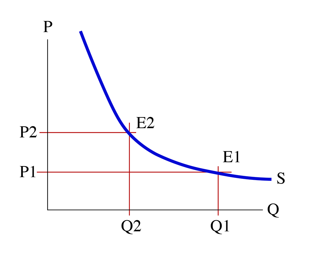
I should comment here that the textbook lumps natural monopoly in with other barriers to entry, and while it can potentially be thought of as a barrier, it is not one that is created by a market-power-seeking firm. Instead, it is a characteristic of a certain type of market - one with high capital costs and low marginal costs.
Given the downward sloping supply curve, and ignoring the demand curve for a minute, let’s say we have an equilibrium at point E1, which corresponds to quantity Q1, and gives us price P1. Let’s assume this is a monopoly equilibrium, where Q1 represents the entire size of the market – it represents everybody who wants to buy the good.
Now, let’s imagine that this was a duopoly market, where there are two suppliers. We can assume, for simplicity, that each seller in the market has exactly half of the market. This corresponds to the equilibrium E2 on the above diagram, which gives us quantity Q2 and price P2. We can assume the , and that each of the two firms supplies Q2 of the good in question.
Do you see the problem? If we have one firm only, the marginal cost of supply is P1, which is lower than the duopoly price, P2. This means that having two firms in a market ends up with the firms having to charge a higher price than if only one firm existed. In this case, it is efficient, or “natural,” for there to only be one firm in the market. This is why declining-marginal-cost industries are called natural monopolies.
What types of industries have this type of structure? Well, generally, industries that have very high capital costs, and comparatively low variable costs. This means that to be the first entrant, you have to spend a large amount on fixed costs, but the cost of servicing an extra customer is very low. Some typical industries would be the delivery of telephone services, or natural gas, or electricity, or cable television. These industries are typically referred to as “utilities,” and they require the development of large infrastructures to serve the customer base. For example, if you have a natural gas distributorship, you have to build a large network of distribution pipes and valves covering an entire city. This represents a pretty massive capital (or fixed) cost component, but the cost of servicing a new customer is very small compared to that.
Now, imagine that this was a competitive market. If there was to be competition between different natural gas suppliers, then there would have to be two sets of distribution pipes. Each firm would have to spend a lot of money, but then compete for the same size of customer base. Each firm would have to spend the same amount of money, but have half of the size of market to try to recover their costs from. Therefore, it makes sense for there to only be one firm in each city – it would be economically inefficient to have two competing natural gas distribution grids, just as it would be inefficient to have two redundant electricity grids, or two telephone grids, or sets of water distribution pipes, and so on.
The Problem of Natural Monopoly
Because natural monopolies tend to be utilities, which are services like gas, electricity, water, and telephones, which the public generally holds to be necessities of life, we are not comfortable allowing these firms to charge monopoly prices (i.e., the pricing where ). Because these are staples or necessities, the demand curve for these goods is very inelastic – it is very steep. This means that the monopolist price would be much higher than the free-market price, and a large volume of people would be denied basic necessities of life. Instead, we use the power of government to regulate prices in these markets.
The normal avenue for regulation of natural monopolies is the public utilities commission. These exist at the state-level in the United States, and at the national level in many other countries. Utilities commissions are given the task of making sure that utility companies make enough money to stay in business, but not enough to enjoy monopoly profits. They make sure that everybody is served, and served well, in theory. Since utilities are monopolies that are not subject to market forces and competition, they have little pressure to be responsive to market forces, which means that they do not have to treat their customers well, because their customers do not have the ability to switch to a different supplier.
In an ideal, perfectly competitive market, we expect price = MC. So, if we were the government power, we might want to regulate the utility to this point. Unfortunately, in a natural monopoly, this would lead to failure of the firm, because of the notion of declining marginal cost. If the firm was paid the marginal cost of the last unit sold for all units (that is, if the law of one price were to apply), then they would lose money on every unit sold, and, inevitably, fail. Another way to say this is that the marginal cost is always lower than the average cost, because the cost of the next unit is lower than all of the previous units made. For a firm to be able to survive in a natural monopoly, it must be able to charge at least the average cost.
Therefore, the goal of the utility commission is to make sure that a utility is able to charge no higher than average cost. However, most utilities are private companies (although some are owned by local governments in many parts of the world), and as private companies they strive to maximize profits. Typically, a private utility will file what is called a “rate case” to a utility commission, which is basically a statement of what the utility needs to earn in order to stay in business and ensure reliable service. It is the role of the utility commission to examine the rate case and see if it believes that the utility is exaggerating its costs. One of the problems of regulating a utility is that they usually are allowed to earn a certain percent accounting profit on their capital base. That is, the larger the capital base (the more buildings and pipes and power plants, and so on) that a utility owns, the more money it is able to earn. For this reason, utilities tend to be “over-capitalized”- they build more capital than would exist in a competitive market.
Another of the benefits of competition is that it drives innovation and efficiency: firms are always trying to come up with smarter and cheaper ways of doing things. While such actions lead to private gains in the near-term, they tend to be beneficial to society over time, as firms make profits and reinvest these into other productive uses. In a monopoly, these pressures also exist to some extent – if a firm can be smarter, it can make more money at the same market prices - but it is totally absent in a rate-regulated natural monopoly, since firms are allowed to earn a certain amount of money by the Public Utility Commission and any extra money they earn must be returned to the public. While such a result is good for the public, it is not for the utility, and therefore, the utility is unlikely to be particularly innovative or efficiency-driven.
The biggest issue in utility regulation today is the question of how to incentivize innovation in utilities, especially when public watchdog groups keep a close eye on what happens at utility commission meetings and protest loudly if they think the commission is allowing the firms to earn too much money, or include too much into the rate base. If a utility wants to spend any money on research and development, they must get approval from the commission, which will then allow the firm to recover the costs of that research. This means that electric or gas or water rates will be higher than they would be without the R&D spending, and members of the public complain if their rates go up. In many places, utility commissioners are elected by the general public, and they usually wish to be re-elected. This means that they want to keep the public happy, and they best do this by keeping rates low. So, we are stuck in a circle of bad incentives that leads to technical stagnation and a lack of innovation.
We will spend quite a bit of time talking about this when we look deeper at the issue of government failure in a few weeks.
Former Natural Monopolies
The above statements about lack of innovation and competitive pressure do not mean that natural monopolies are immune to technological innovation that weakens their market power. Instead of having multiple firms compete to provide a single service, instead, we now have competing technologies attempting to provide the same service. The most obvious example is that of telephones. It used to be that the telephone system, or at least the part of it from the end user to the phone company’s switching and transmission points, was fully hard-wired. The local phone company had to build a network of cables connected to every house, usually at very high cost, a cost that could only be recovered by either charging monopoly prices or having regulated profits. It was a classic natural monopoly, and one that is government regulated or government-owned in many parts of the world. However, new technology was developed that allowed that last piece of wire between the customer and the phone company to be replaced by radio signals. Thus, we have the cellular phone, and competition with the land-line telephone. People no longer have to rely upon the old-fashioned phone company for their voice communications needs. The same is true of cable television and satellite TV, and now we can get Internet services delivered by the cable company or the phone company or the cell-phone company. Thus, the list of markets that can be classified as natural monopolies has shrunk in recent years. We have yet to find competitive alternatives for electricity, natural gas, and water, and markets for these products remain tightly regulated.
Information Market Failure
Required Reading
Please read pages 103-106 in Chapter 5, the segments entitled "Potential information Problems" and "Information as a Profit Opportunity." This is in the chapter entitled "Difficult Cases for the market, and the Role of Government."
Perfect information is one of our assumptions of perfectly competitive markets, and it is easy to see that this assumption is perhaps the toughest one to make, simply because perfection is something that does not exist. Information can have many aspects in a market setting. The foundation for our analysis of demand in markets is the idea that people are able to place value on the consumption of goods, on understanding the amount of happiness they will obtain from the economic decisions they make. Since the realization of many of our economic decisions takes place in the future, and because the future has an unknown component, it is basically impossible for us to have perfect knowledge without perfect foresight – and that is something we do not have, and cannot have.
However, as a market failure, this is not something we can correct. We can, as individuals, educate ourselves about the world and what sort of outcomes we can come to expect. We can gain wisdom and insight, but we can never tell the future with certainty. Thus, we will consider this issue further. It is merely a manifestation of the nature of our existence and the linear nature of time.
Instead, we need to concern ourselves with information that is knowable, but the lack of knowledge by one or another party in an economic transaction causes a loss of wealth to society.
Some markets have close to perfect knowledge of present information. Perhaps the best example is the market for shares of widely traded public companies at places like the New York or London stock exchanges. The shares are all homogeneous – one share is exactly the same as another, the prices are readily available, in real-time, to anybody who is interested, and there are many, many people studying the activity of the companies that are being traded. Because they are publicly traded on stock exchanges, these companies are required to release a lot of information to the public about their business activities, their profitability, their debt levels, and so on. Generally, a person buying a share in a large public company like IBM or General Electric or Exxon knows or, at least, has the ability to know, about as much as anybody else in the market for the share in question.
There is one situation where somebody might know something about a company that the general, investing public does not: when a person is an “insider,” and has some non-public knowledge about the future of the company. A manager or director of the company may know that they are in the process of planning a takeover of another company, or are being taken over, or are about to suffer a large loss due to some non-public event. The announcement of such pieces of information can have significant effects on the price of shares of these companies. Thus, insiders can profit greatly by buying or selling stock using information that is not available to the general public. This is what is referred to as an “information asymmetry.” For this reason, insider trading of stocks is highly regulated in many countries. Insiders – managers and directors – have to make public record of their stock trades, and if a material event happens that they can reasonably be expected to have had inside information on, the securities authorities will examine the history of their trades to make sure that they did not profit from that knowledge unfairly. If they are found to have done so, they can be severely punished. In other countries, for example, Germany, the securities authorities make sure that all insider trades are publicized immediately, so that the general public can mimic them. The authorities in countries like this assume that this is a better way to disseminate information about what is going on in markets and in industry. If insiders are making big moves, and people can see them, the market will assimilate that information quicker than it otherwise would. At least, that’s the theory. If you go ahead and study finance, this is what is called the strong form of the efficient markets hypothesis, about which there is a great amount of disagreement in academic and professional circles.
The last type of information market failure concerns another type of information asymmetries: that about products or services being sold. It is not hard to realize that, typically, a seller of a product knows a great deal more about that product than the buyer. Sometimes, a seller will use this to his advantage by not telling the buyer something meaningful and important about the product. This is sometimes referred to as getting “ripped off.”
When will a seller take advantage of such a situation and “rip off” a consumer? The short answer is: when it pays to do so. More specifically, there are some conditions:
- When you can’t find out that you are being cheated until after the purchase is made, and
- When you can’t punish them once they’ve cheated you:
- When you only make a single purchase from the seller. For example, most people only purchase a house a few times in a lifetime and very rarely more than once from the same seller.
- When there is only one seller. If you feel like you’re getting ripped off by the power company or the only gas station for 20 miles, you cannot easily take your business elsewhere.
- When getting cheated is a small enough loss to not change your preferences.
- When you will never find out if you have been cheated. One example of this is people undergoing unnecessary surgery. This why they say you should always get a second opinion.
So, summing up, sellers will have an incentive to cheat buyers when buyers cannot adequately punish sellers.
Consumers can also take advantage of suppliers — moral hazard. The best example of this is insurance:
- a) Insurance companies agree to pay your damages after an accident.
- b) However, they do not control your behavior, and you have incentives to be risk-loving, knowing your damages will be paid.
Another example is academic integrity:
- a) Most teachers believe that you hand in your own work and don’t go to great lengths to certify that what you hand in is yours.
- b) However, they cannot control (or costlessly discover) whether you have done the work yourself, or copied from a friend.
Of course, when insurance companies (or teachers) catch you, consequences are usually significant.
Correcting Information Market Failure
In this case, there are private as well as public (governmental) solutions:
- Trade Organizations: If a company misbehaves, their reputation will be hurt and the trade organization will cease to support them.
- Consumer Organizations: Publications like Consumer Reports independently monitor companies’ performance and keep consumers informed.
- Anti-Fraud Legislation: If you can prove a company cheated you, they will have to pay restitution to you and prohibitive damages to the government.
Summary and Final Tasks
In this lesson, we looked at some of the other types of market failure that can exist. Firstly, we talked about one of the manifestations of the violation of the assumption of free entry and exit, that being the way in which some incumbent sellers in a marketplace try to erect barriers to entry into a market, which helps reduce the amount of competition a firm faces, whether it is a monopoly or not. There are various barriers to entry, some supported by government, some illegal, and some perfectly legal. We then talked about natural monopolies, which are typically utilities, in which it makes sense from a standpoint of economic efficiency to have only one supplier in each market. The last section was about the violation of the assumption of perfect information. We spoke of some ways that asymmetric information can be used to gain an unfair advantage in a marketplace, and when and why this information can and will be used.
Have you completed everything?
You have reached the end of Lesson 6! Double check the list of requirements on the first page of this lesson to make sure you have completed all of the activities listed there.
Tell us about it!
If you have anything you'd like to comment on or add to the lesson materials, feel free to post your thoughts in the discussion forum in Canvas. For example, if there was a point that you had trouble understanding, ask about it.
Lesson 7 - Externalities and Environmental Economics
Lesson 7 Overview
In this lesson, we reach the end of the topic of market failures. The last market failure mechanism for us to address, which is perhaps the most important to the topics of energy and sustainability, is the market failure known as an "externality," which is a violation of the assumption of free entry and exit into a market. The most important type of externality is the existence of air and water pollution. In this lesson, we will take a look at how we can use economics methods to "internalize" externalities. We will also speak of goods that are under-provided or over-exploited in an uncontrolled marketplace due to the absence of well-defined property rights.
What will we learn?
By the end of this lesson, you should be able to:
- define what an externality is;
- list and describe some examples of externalities;
- explain the difference between private and social costs;
- draw a diagram showing the private and socially optimal equilibria, and the private and social cost functions;
- show how we can define and get to the socially optimal equilibrium given a schedule of utilities/costs for each party;
- explain the fundamentals of the Coase Theorem;
- describe situations where the Coase Theorem does not work well;
- describe different approaches to pollution control;
- describe and explain the merits of different approaches to pollution abatement.
What is due for Lesson 7?
This lesson will take us one week to complete. Please refer to Canvas for specific time frames and due dates. There are a number of required activities in this lesson. The chart below provides an overview of those activities that must be submitted for this lesson. For assignment details, refer to the lesson page noted.
| Requirements | Submitting Your Work |
|---|---|
|
Read Chapter 5 in Gwartney et al., OR Chapter 12 in Greenlaw et al. Plus other assigned readings linked to in the lesson text |
Not submitted |
| Lesson Quiz and Homework | Submitted in Canvas |
Externalities
Reading Assignment
For this lesson, please read the sections entitled "Externalities - A Failure to Account for All Costs and Benefits," "External Costs," and "External Benefits" in Gwartney et al. Chapter 5 - "Difficult Cases for the Market." Or read Greenlaw et al. Chapter 12
“Externalities” are the last type of market failure we will talk about. They are a form of free entry/exit market failure. When a trade is made, there are normally two people affected by the trade: the buyer and the seller. But, sometimes, a trade or some other piece of economic activity has an effect on people who are not directly involved. Because these effects are on a person who is external to (or outside of) the trade, we call them externalities. Externalities can be either positive or negative; that is, the economic activity of one person or group can have either a positive or negative "spill-over" onto other people.
An externality is when the welfare (utility) of a person depends not only on his activities, but also on the activities of an “outside” person. An externality exists whenever an individual or firm undertakes an action that impacts another individual or firm for which the latter is not compensated (a negative externality, e.g., pollution), or for which the latter does not pay (a positive externality, e.g., voluntary vaccination). This occurs when property rights are NOT well-defined. When externality exists, the competitive market does not achieve the efficient allocation of resources in society (i.e. the market fails) because no market exists in which the affected party can express his/her preferences for the externality. The presence of externalities means we are ‘missing a market’ for the externality. Because externalities are often co-produced with other market transacted goods (e.g., emissions and electricity) this distorts the markets of the transacted goods as well as the markets connected to them.
Examples of externalities:
Pollution
This is the most common type of externality, and the one that will be addressed most frequently in this course and in real life. It can take many guises. For example, think about a case where a village makes its living from catching and selling fish from a river. Now, if a chemical plant opens 25 miles upriver and decides to discharge chemical waste into the river, then the fish all die and the people in the village lose their ability to make a living. In this case, the chemical plant (and, by extension, its customers) is not being forced to cover all of the costs of its operation. If it was required to dispose of hazardous waste in some way that did not involve dumping it into a river, then it would be faced with higher costs, and if it has higher costs, then the price of its products will be higher. If the price is higher, then consumers will purchase less.
Air Pollution
Air pollution is one of the key externalities that has been addressed in the US over the past 40 years. And coal has been the largest source of some of the worst air pollution. In 1998, coal power plants were responsible for:
- 67% of Sulfur Dioxide (SO2)
- 33% or Mercury
- 35% of Nitrous oxides (NOx)
- 40% of GHG emissions (CO2, methane, etc.)
- Particulate Matter (PM)
In the Industrial Heartland of the US - places like Michigan, Ohio, and Pennsylvania - a lot of industrial facilities have burned coal over the past 150 years. The coal that is burned in these power plants, steel mills, and factories contains sulfur. When sulfur burns, it forms a compound called Sulfur Dioxide, SO2. The SO2 is carried into the environment by the exhaust stacks connected to the boilers of these plants. When the SO2 mixes with water vapor in clouds, it forms Sulfuric Acid, H2SO4, and eventually, this falls as part of rain. This is what is known as Acid Rain, and was responsible for lowering the pH of many lakes and rivers in the north-eastern part of the United States to the point where these bodies of water were unable to sustain any life. Another form of air pollution comes from the burning of gasoline in motor vehicles, which gives us several undesirable compounds: unburned hydrocarbons and partially reacted oxygen, in a form called ozone, which, in the presence of sunlight, creates photochemical smog, which can be severely damaging to the lungs. We also get particulate emissions - another word for soot - which consists of very fine particles of partially burned hydrocarbon that float in the air and get inhaled by people, and we also get Carbon Monoxide, a poisonous gas that can cause nausea at low concentrations and death at not so high concentrations. These emissions have all been the target of environmental legislation over the past 40 years, and we will talk at length later of attempts to regulate them.
Water Pollution
A common form of water pollution is runoff of fertilizer from fields. In the central part of the US, known as the "Bread basket" (think of places like Illinois, Iowa, Kansas, and so on), farmers use a great amount of chemical fertilizer to ensure large crops of corn and soybeans. Since fertilizer is relatively cheap, farmers have an incentive to over-apply, as opposed to under-applying it. Any fertilizer that is not absorbed by the plants runs off with rainfall into rivers, and these rivers all end up flowing into the Mississippi River. As you go downstream, the concentration of the Mississippi river increases. The result is that in the Gulf of Mexico, just off the coat of Louisiana, there is a large "dead zone' several hundred square miles in size which is caused by the excess fertilizer in the water. This fertilizer accelerates the growth of algae in the water, and the algae consumes all of the oxygen in the water, meaning that nothing else can live in the water. One of the reasons that the damage from the recent oil spill in the Gulf was not larger was that it occurred in this "dead zone," so there was not a lot of marine life to kill to begin with. This situation creates a benefit for everybody who consumes corn or soybeans - which is, basically, all of us, in the form of cheap food, but it has a significantly negative effect on the biodiversity of the Gulf of Mexico, with secondary effects that are scarcely understood by humans.
Bees and Crops
This is an example of a positive externality: bee keepers take part in a market for honey; they raise and keep bees in order to harvest honey and sell it to the public. In the process of creating honey, bees fly around and pollinate plants, which enables them to grow. This is very beneficial to people who grow flowers and vegetables for a living. Without bees, these vegetable or flower growers would have to manually pollinate their plants - a very tedious and labor intensive process, or develop hybrid plants that are self-pollinating. These are both costly propositions. Indeed, these businesses rely upon the presence of bees to enable their business models to work - without them, their products would be more expensive, and thus there would be less consumed. So, the presence of bees to pollinate commercial plants is a positive externality that arises from the presence of honey farmers.
Noise
Pollution does not simply refer to dirty air or water, but it also refers to other bespoilments of the environment, and one of these is noise pollution. Noise pollution can come from a variety of sources: highways, airports, factories, construction sites, nightclubs, railroads. (I live close to a railway level crossing, and the sound of sirens and horns as the trains pass the crossing several times a day can be very annoying. Fortunately, one grows accustomed to this noise, and after a while, you don't really hear it.) It is basically another by-product of economic activity, and if the noise was forced to be reduced in some way, then the firms generating it would have one of two choices: reduce the amount of economic activity (this is common, such as airports being forced to be closed overnight), or install expensive equipment to reduce the amount of noise emitted. Once again, this has the effect of raising costs, and the raising of costs means that the equilibrium price is higher, and there will be less consumed. Sometimes the economic activity gets shut down completely - for example, a lot of bars and clubs in New York City have been forced to close because the buildings they occupy have become residential areas, and the clubs get fined for excessive noise so frequently that they are unable to continue doing business.
There can be positive and negative externalities, but since positive externalities do not present a large economic problem, economists concentrate on negative ones - positive externalities do not really present much of a market failure issue.
The general issue here is one of costs: there are costs that are borne by the participants in the economic transaction, and then there are costs that are borne by non-participants - the external costs. The costs that the participants bear - the costs to the seller that are transferred to the buyer via the price mechanism - are what we call "private" costs. In an ideal world, all economic costs will be private - they will be all borne by the people who derive utility from the transaction. However, in reality, there are many cases where there are some costs that are transferred to non-participants - such as fisheries destroyed by acid rain, or the ill-health that comes from breathing dirty air, or the problems of trying to sleep near noisy factories or railroads. These costs, which are not carried by the manufacturer or purchaser of the goods in question, are what we call "social costs," because they are borne by society. They are illustrated in the following supply and demand diagram:

In the above diagram, we have the "private" equilibrium (Q1, P1), which is the intersection of marginal private costs (MC) or supply curve (for example marginal cost of producing each kWh of electricity) and market demand. We also have the "social" equilibrium (Q2, P2), which is the intersection between Social Marginal Cost and demand curve. Social Marginal Cost is the sum of marginal private plus Marginal External Cost (Social Cost). We can define the Marginal External Cost (MEC) as for example the additional external cost from each additional kWh of electricity that is produced. We can assume the Social Marginal Cost a line parallel to the marginal private costs but above that, because it bears the social cost (for example cost of harm to the people).
The difference between these two equilibria comes from the upward shift of the supply curve when we include the social costs, which are costs that are paid by society in general, or by people "external" to the transaction, versus the private supply curve, which is the one that contains all the private costs. Therefore, "social" equilibrium would be at higher price and lower quantity. It should be clear that the true social optimum is not (Q1, P1), but instead (Q2, P2) once we account for the costs of the negative externality on society. Note that the competitive equilibrium leads to too much pollution being produced and less total wealth. If we ignored external costs from producing electricity from coal and consumed at (Q1, P1), we would obtain gains in consumer and producer surplus equal to the green trapezoid, however we also incur marginal external costs equal to the purple parallelogram. So, society experiences a wealth loss equal to the blue triangle.

I may be over-simplifying things here, but, basically, the entire field of environmental economics is concerned with trying to shift the equilibrium from the private one, (Q1, P1), to what we call the "socially optimal" equilibrium, (Q2, P2). This is often referred to as "internalizing" an externality.
In the next lesson, we will discuss methods for performing this shift, how these methods are implemented, and how effective they are.
What is not an externality?
When we talk of one person's actions affecting another person negatively, we sometimes hear about something called a "fiduciary externality." This can be boiled down to the following: if one person buys a good, they are moving the demand curve outwards. This act of moving the demand curve outwards will result in movement of the equilibrium to a point where the price will be higher than it would be without that person buying. Put another way, if I buy a good, you cannot buy it, and if you want to buy it, you may have to pay a higher price. This is most obvious in an auction scenario. Just last night, I was watching an auction for exotic cars, and, in one case, there were two bidders for a certain vehicle. Each person kept increasing their bid, that is, causing the other person to pay more. This is not a market failure. Another example could be travel at Thanksgiving: because more people want to fly, and because the number of airplanes is finite, fares tend to increase over Thanksgiving. Similarly, more people want to drive over this period, and thus roads are more congested (and thus, the opportunity cost of using them increases). These are all situations where increased demand raises prices, so that any one person is adversely affected by everybody else's economic choices, but this is not an externality in the sense that it is not a market failure - it is merely a dynamic realignment of the market equilibrium as a response to a temporary change in demand, much like the fact that roses are more expensive on February 14th than they are on February 21st, gasoline is more expensive around Memorial Day than around Columbus Day (ceteris paribus), and hotel rooms are a lot more expensive at Rehoboth beach, DE in July than in November. I reiterate: these are not market failures, except in cases where market power comes into play, but that is a separate issue.
Dealing With Externalities
Reading Assignment
For this lesson, please read the section entitled "Public Goods and Why They Pose a Problem for the Market" in Chapter 5 ("Difficult Cases...").
In this lesson, we will describe a real-world use of Coasian policy to deal with an externality and provide an example of how such systems work in general. We will also talk of other methods and why they are less attractive than Coasian methods.
We will now focus on the topic of attempting to reduce the emissions of Sulfur Dioxide (SO2) from power plants and steel mills that consume coal. We previously mentioned why SO2 emissions are "bad" - they create acid rain, which renders lakes incapable of supporting life. Acid rain also damages buildings, as any of you who have been to Pittsburgh can readily see.
There are three general ways in which SO2 emissions can be reduced. These all involve attempting to move from the private to the socially optimal level of pollution. We should note at this point that the socially optimal level of pollution is not zero, but is the point where the marginal benefit of pollution equals the marginal cost.
You might ask, what is the social benefit of pollution? Well, pollution itself does not have any benefit, except perhaps to companies selling pollution-control equipment and to class-action lawyers. However, we need to remember that it is merely a by-product of an industrial process that creates something we find to be very useful: electricity. Without burning coal, electricity would be much more expensive in the US. Therefore, when we consider the benefits of using electricity, we have to consider this as a benefit that comes from emitting SO2 into the environment.
As mentioned above, there are three general ways we can proceed:
1) Command and Control. This is exactly what it sounds like: governments issue commands in order to control the amount of pollution. This approach is simply to require that all firms employ some abatement or emissions control technology or equipment (think “scrubbers”—devices that one can attach to the end of a smokestack to pull out bad emissions from the stack). If emitters fail to comply with these rules, they face criminal sanction and the possibility of fines and imprisonment.
Command and Control approach may involve some distortions:
- Instead of forcing all firms to invest in an expensive scrubber, it may be cheaper for some firms to reduce emissions by purchasing cleaner inputs (e.g., low sulfur coal)
- Plants have different ages and design, can impose unequal cost burdens to firms
- May discourage firms from investing in newer pollution abatement technology (e.g., may need to trash investments if new C&C regulation comes along (often a motivation for firms to push for C&C regulation—in order to reduce regulatory uncertainty)
- Current firms can “capture” regulatory board and require technologies that are easy to implement (or already in place). May serve as a barrier-to-entry to new competition (e.g., Cement).
- Political distortions: a US senator, pushed for mandated scrubber technology so high-sulfur WV coal could compete with low-sulfur PRB coal
Thus Command and Control is unlikely to be the most efficient solution.
2) Pigouvian taxes. These are taxes on pollutants, and got their name from the first person to propose them, a British economist called Arthur Pigou. A Pigouvian tax moves the equilibrium from the private to the social one, but it does so by setting a fixed cost (the tax), and then allowing quantity to adjust in the marketplace. The problem with this system is that it requires more information. If the tax is too high, the quantity emitted will move to a quantity below the socially optimal value, which means that some wealth is destroyed. If the tax is too low, then we will not reduce pollution by very much, and we will be producing at a level above the socially optimal amount, which is also not a wealth maximizing situation.
3) Coasian permit trading. This is a system whereby the government delegates to itself the property right to emitting sulfur dioxide and then sells (or gives away) these property rights. A company needs a permit for every ton of SO2 they wish to emit into the environment, and the quantity of those permits is controlled by the government. This method has the benefit of allowing firms to trade permits so that firms that have a high cost of emitting can buy rights from firms that can reduce pollution at lower costs, which means that as a society we can have the same amount of pollution reduction as in the command and control method, but at a lower cost to society. This will be illustrated a little later. This method is called "cap and trade," because the government will set a cap on the amount of SO2 that can be emitted each year and then allow emitters to trade amongst themselves to obtain the socially efficient result. Cap and trade contrasts with Pigouvian tax method in this way: with a Coasian system, we are setting the socially optimal quantity, and then allowing the price to find the market equilibrium. In theory, this is equivalent to the "social cost," the difference between the two supply curves in our social versus private equilibrium diagram. The good thing is, we do not have to try to figure out this cost, which can be extremely difficult to discover, but, instead, we can simply let the market find the level. Cap and trade method seeks to creates a market for externalities. This a possible solution to the missing market problem of externalities. Once we create a market for the externality, it is no longer external to the market. Hence we say we have “internalized the externality.”
So, in theory, all three methods get the same results, but, in reality, the cap-and-trade method can be shown to work better than either alternative.
The first attempt to limit sulfur emissions, the Clean Air Act of 1970, used command and control regulation, and relied upon government to specify and administer all aspects of pollution control (i.e., micro-management). The Environmental Protection Agency (the EPA), the government agency charged with administering environmental policy, would determine performance standards applicable to each pollution source. Typically, standards were set in rates: quantity of pollution emitted per hour, or per unit-of-energy, etc. Sources then would have to find a way to meet these fixed, general standards. Each could choose one of two methods of compliance:
- Install pollution control equipment
- Reduce the number of hours of production (in the extreme, shutting down completely)
Both of these methods of compliance are very expensive. Old plants have high emission rates (because they were designed without pollution control in mind) and need to install A LOT of pollution control equipment to come into compliance. According to the law of diminishing returns, each next unit of pollution reduction costs more than the previous unit. This translates into HUGE costs to old sources, and huge costs for middle-aged sources. Another large cost comes from the fact that most industrial facilities are very valuable to society - in the hundreds of millions of dollars each. Completely abandoning a facility, even if it has been paid for, necessitates construction of a replacement facility. As a result of these high costs, industry would choose to endlessly litigate new environmental policy in the courts rather than comply, and the environment was never very adequately protected. The Clean Air Act of 1970 required all coal-fired plants to install pollution-control devices called "scrubbers," but the legal fight back was great - to this day, 40 years later, the majority of power plants built before 1970 still do not have scrubbers.
The result was that by the end of the 80s, the rates of SO2 emission were still much higher than what was thought to be the socially optimal amount, and acid rain was still a problem. At the urging of economists, the government adopted a different approach, one consistent with the teachings of Coase. In the Clean Air Act Amendments of 1990, Congress adopted a cap and trade program for sulfur dioxide, known as the Title IV program, based on the chapter in the law.
Under Title IV, every year, the EPA would decide how many permits were to be issued. This number shrank every year. The number started at about 17.3 million tons in 1991, and was down to about 9 million tons/year by 2000. The EPA would allot the permits to plants based upon their emissions in some base year, and the firms could either emit SO2 and surrender permits to the government, or it could sell the permit and then release less SO2. This aligns the incentives of the firms with the goals of reducing pollution - it would award firms for innovating and reducing pollution by being able to "sell," and hence benefit from, their pollution control efforts.
The accounting behind this system is very complex, so I will use some simple numerical examples to illustrate how such a system works.
Let us say that there are three firms: Awful Industries (Firm A), Bigbaddirty Inc (Firm B) and the Crud Corporation (Firm C). In the beginning of our problem, there are no pollution laws, and each firm is polluting at their maximum level. For each firm, this is 5 tons per hour. The air is getting terribly polluted, and the government hires a group of biologists, who say that there should never be more than 9 tons per hour emitted.
1. Using Command and Control
Firstly, the government decides to limit each firm to 3 tons each. The following are the firm profits at each level of pollution:
| Units of pollution | 0 | 1 | 2 | 3 | 4 | 5 |
|---|---|---|---|---|---|---|
| Firm A | 0 | 100 | 190 | 270 | 340 | 400 |
| Firm B | 0 | 150 | 270 | 360 | 420 | 450 |
| Firm C | 0 | 160 | 240 | 280 | 300 | 310 |
From Table 7.1, we can see that each firm makes the maximum profit at 5 units of pollution, so that is what they will do if there are no controls - emit the maximum amount. This is because reducing pollution costs money: firms have to spend to clean up their waste, and they are not able to produce as much stuff. Another way to look at this is to reverse Table 7.1 and look at the TOTAL COSTS of reducing pollution (this is also called “Pollution Abatement”):
| Units of pollution | 0 | 1 | 2 | 3 | 4 | 5 |
|---|---|---|---|---|---|---|
| Firm A | 400 | 300 | 210 | 130 | 60 | 0 |
| Firm B | 450 | 300 | 180 | 90 | 30 | 0 |
| Firm C | 310 | 150 | 70 | 30 | 10 | 0 |
Table 7.2 tells us how much it would cost to move from the uncontrolled situation to a certain amount. For example, if Firm A had to move to 1 unit, they would have to give up 300 in profit.
In order to calculate the numbers in table 7.2, we can start from the last column and move to the left. The last column to the right is when firms make no effort in reducing units of pollution. In that case, the total cost of pollution reduction is zero. Then, we move to the next column, where firms reduce only one unit of pollution (producing 4 units of pollution each). Total cost of reducing only one unit of pollution can be calculated as: (total profit at 5 unit of pollution) – (total profit at 4 unit of pollution). The next column (moving to the left) is when each firm produces only 3 unites of pollution (removing 2 units). We can calculate the total cost of producing only 3 unites of pollution as: (total profit at 5 unit of pollution) – (total profit at 3 unit of pollution). And if we continue this method to get to the first column, we will have Total cost of producing zero unit of pollution = (total profit at 5 unit of pollution) – (total profit at 0 unit of pollution).
So, what are the costs to the firms if they are each forced to emit only 3 tons each? Well, we just add up the total costs in the column headed by “3 units.” The total loss is . Remember this number.
This is the same as the government giving 3 pollution permits to each firm, and telling the firms that they may not trade the permits amongst them.
2. Cap-and-Trade
What if the government gives three permits to each firm, and says that the firms can trade them? Well, Firm A will make 70 more in profits if they can pollute 4 units. Firm C will make 40 less units of profit if they go to two units. So, we have a potential trade. Firm A is willing to pay up to 70 for an additional permit, and Firm C is willing to accept more than 40 for a permit. Since we can find a mutually beneficial amount between 40 and 70, then the trade will happen. This means that Firm A will now emit 4 units (because it has 4 permits) and Firm C will emit 2, as it now only has 2 permits.
The result is that we will have Firm A polluting 4, at a total cost of 60, Firm B will still pollute 3, at a total cost of 90, and Firm C will pollute only 2 units at a cost of 70. So, the total cost for all three firms is now .
So, now we have the same amount of pollution, but the total cost to the firms is reduced from 250 to 220. This benefits society: either the firms can make more profit, or they can lower their prices. Both of these things are good for the economy.
There is one more benefit to having a permit system: if a person wants to reduce pollution, all they have to do is buy a permit and then not use it. This reduces the total amount of pollution in the world.
In this market, permits will trade for between 40 and 70. If we have a larger market, with more firms, we can expect more trades and we can expect the equilibrium price for permits to converge to a single value. This value will be the value of the Pigouvian tax we need to have the same result, but, as I mentioned above, this would likely require quite a bit more trial-and-error on behalf of the tax-setter. Simply setting a cap and letting the price equilibrate based upon firms trading in their own best interest is a more effective way to reduce pollution.
A Tale of Two Roommates
Here is a story about two guys sharing an apartment. We’ll call them Bert and Ernie. It turns out that Bert is a big fan of Megadeth, and can't get enough of their music. However, Ernie does not like this music so much. Ernie likes quiet. So, we have a bit of a problem: two people sharing the same apartment, one who likes loud, raucous, heavy metal, and one who cherishes peace and quiet. Is there a solution? This being an economics course, we are inclined to ask, is there some application of “economics” that would allow us to define just how much music can be played and keep both people happy? Is there some way we can "optimize the social wealth" in the apartment, some way to maximize happiness in the entire in-apartment community, which consists of Bert and Ernie. (We'll not worry about any externality effects the music might have on the neighbors for now.)
Well, in economics we are fond of stating things, especially utility and happiness, in terms of money, if only for the ease of accounting and measurement it allows us, so we have to define Bert and Ernie’s “happiness” in numbers. These numbers represent happiness in money terms. Let us suppose that the happiness for between zero and 5 songs is given on the following table:
| Number of songs played | Bert's Happiness | Ernie's Happiness |
|---|---|---|
| 0 | 0 | 0 |
| 1 | 10 | -2 |
| 2 | 18 | -6 |
| 3 | 24 | -13 |
| 4 | 28 | -20 |
| 5 | 30 | -32 |
The above table contains the "total" amount of happiness for each number of songs. As you can see, the more songs played, the happier Bert gets and the more unhappy Ernie gets. We can assume, for simplicity, that all of the "happiness" numbers are denominated in dollars.
What is the “best” number of songs? Well, we want to know at which number total social happiness is maximized. Since our society here consists of two people, it's pretty easy to do - we add together everybody’s happiness and find out what the highest total is for everybody added up:
| Number of songs played | Bert's Happiness | Ernie's Happiness | Total Happiness |
|---|---|---|---|
| 0 | 0 | 0 | 0 |
| 1 | 10 | -2 | 8 |
| 2 | 18 | -6 | 12 |
| 3 | 24 | -13 | 11 |
| 4 | 28 | -20 | 8 |
| 5 | 30 | -32 | -2 |
So it appears that 2 is the “best” number of songs played. It is the “socially optimal” amount.
Now, how do we get to this amount?
Let us assume that this apartment belongs to Bert, and Ernie is his guest. So Bert has the “property right” to play music. Since he has the right, and he is happiest when playing 5 songs, then this is how much he will play in the beginning.
This being economics and all, Ernie decides that maybe he can buy a little bit of peace and quiet. So, he offers Bert some money to go from 5 songs to 4. If we go to 4, Ernie's happiness increases from -32 to -20, so he is 12 dollars better off. So, he would be willing to offer up to 12 for one less song. If we go from 5 to 4, Bert's happiness decreases from 30 to 28. He will be giving up 2 dollars of happiness to listen to one less song. So, if he is being offered more than \$2 to not play the 5th song, he should accept if he is a rational utility maximizer, and, of course, we assume that he is. For this drop in music, he must gain back at least \$2 to be better off. So, we will have a trade. Ernie will pay less than 12, but more than 2, to go from 5 songs to 4. Both guys are happy with between 2 and 12 dollars being exchanged for one less song.
We can repeat the same thing for 4 to 3 songs and 3 to 2 songs.:
From 5 to 4 songs, the payment is between \$2 and \$12
To go from 4 songs to 3 a payment of between \$4 and \$7 will satisfy both Bert and Ernie.
Now, if we have negotiated a total of three songs, and Ernie wants to go down to 2, he will offer up to 7, and Bert will accept anything over 6.
So, to date, we have had three opportunities to make trades where both people are better off - Bert is willing to give up music if he is compensated more than the happiness he is losing from not hearing music, and Ernie is willing to pay if he pays less than the amount of happiness he gains from each less song. These trades are mutually beneficial, and are "wealth generating" - both guys are better off if these "trades" are made.
So, what about going from 2 to 1 song? Well, to do this, Bert needs to get at least \$8, because that's how much value he places on the second song. However, Ernie is only willing to offer 4, since that is how much he values the extra silence. Since there is no number that is above 8 AND below 4, this trade will not be made. We will stop at 2. So, if we add up the trades, we can say that:
“We will go from 5 songs to 2 for an exchange of between \$12 and \$26.”
Note that we stop at 2 songs, which is the “socially optimal” amount.
OK, now what if we assume that the opposite is true: that Ernie owns the flat, and Bert is his guest. In this case, Bert is happiest with 0 songs. So, that is where we start. In this case, Bert is willing to offer Ernie some money in order to be able to play some music. To go from 0 songs to 1 song, he will offer up to 10. Ernie will be happy with anything more than 2.
So, we will go from 0 to 1 songs with a payment between \$2 and \$10. This will be a mutually beneficial trade, so both are willing to make it.
Now, if we want to go from 1 song to 2 songs, Bert is willing to offer up to \$8, and Ernie is willing to accept anything over \$4. Once again, there is an opportunity for a trade to be made, and it will be made.
So, what about going from 2 to 3 songs? Well, Ernie needs to get at least \$7 to want to do this trade. However, Bert is only willing to offer \$6. Since there is no number that is above 7 AND below 6, this trade will not be made. We will stop at 2. So, if we add up the trades, we can say that:
“We will go from 0 songs to 2 for an exchange of between \$6 and \$18.”
Note that we stop at 2 songs, which is the “socially optimal” amount.
You will notice that we started in two different places - in one case we started with 5 songs being played and, with voluntary exchange, we got to 2. In the other case, we started at 0, but with mutual, wealth-generating trades, we also got to 2. No matter where we start, we end up at the same place, and that place happens to be the socially optimal amount of Megadeth tunes.
OK, so this example seems a little silly. But let’s say I changed the table above to “Tons of Hideous Guck Emitted into Stream by Steel Plant Near Your House,” “Payoff to Steel Plant,” “Payoff to People in Your Town.”
Another Example
| Number of Junior Whoppers | PH Total Value | NR Total Value |
|---|---|---|
| 0 | 0 | 0 |
| 1 | 9 | 8 |
| 2 | 16 | 14 |
| 3 | 21 | 18 |
| 4 | 24 | 20 |
| 6 | 25 | 20 |
Paris Hilton and Nicole Ritchie are stuck in a room at the Motel 6 for the next 3 hours. Both are hungry. Paris has a bag of 5 Junior Whoppers, while Nicole has no food. Nicole does have money. Here are their TOTAL value of Junior Whoppers. All values are in \$ million
Assuming that Nicole does not use force, and that neither party acts out of spite (ok, let’s pretend), explain any deal that will take place. Some hints: 1) Calculate marginal values; 2) Remember, don’t have the sum of Junior Whoppers that Paris and Nicole eat exceed 5!
Practice Exercise:
Eric and James are locked in the locker room at the Jordan Center for the next five hours. Eric has 6 “mini-Mac” burgers in a bag. James has money. Each of them has total value of mini-Macs consumed (in shekels, of course) as outlined below.
| # of Macs | Eric's Valuation | James's Valuation |
|---|---|---|
| 1 | 40 | 90 |
| 2 | 70 | 160 |
| 3 | 95 | 215 |
| 4 | 116 | 265 |
| 5 | 131 | 301 |
| 6 | 140 | 333 |
A: Assume that neither party acts out of spite, and all trades are voluntary, explain what trades will be made.
B: Let us make this a little harder. Assume that every time Eric sells a mini-Mac to James, Eric has to pay 50 shekels to the government authority. How many shekels will the government collect from Eric, and why?
The Coase Theorem:
If transactions costs are not “too high,” the market will find the optimal (best, wealth maximizing) solution.
But what constitutes “transactions costs?”
What could be a transactions cost?
- Spite. Perhaps not so much in business, but often in divorce (“The War of the Roses” (1989))
- Government Regulation and taxes; say a tax on trading
- Public goods problem. Instead of having only Ernie being affected by the toxins in the stream, let us have 100,000 residents in your hometown being affected. Now, fighting pollution becomes a public goods problem. (So, the problem with externalities is that they create public good problems. We will learn more about public goods in following lessons) Here the government could come in and impose a solution. The government could say: Don’t pollute so much; or pay us X dollars every time you pollute. What is the difference?
This theory was first elaborated by a professor by the name of Ronald Coase, who won the Nobel Prize in Economics for his work in 1991. He was the first person to observe that if property rights were well defined, and could be enforced, it was possible for a society to move to the socially optimal equilibrium in cases of pollution, or other externalities. In his honor, this has become known as the "Coase Theorem," and is the foundation of a large part of environmental legislation in the United States.
Want to learn more?
If you are a little bit more interested in this, you can read the article at the following link, which was written at the time of Coase being awarded the Nobel Prize. It is written at a slightly higher technical level than most of the course content, but is not so obtuse that anyone taking this course should have difficulty reading it.
"The World According to Coase" by David D. Friedman
The most important underlying assumption of using a "Coasian" solution to an externality problem is that property rights need to be well defined and enforceable. That means that we have to know who owns what, and that the people who own those things should be able to enforce their rights, and stop unauthorized users from using resources that they own. After a little bit of thinking, this becomes self-evident. Externalities arise because an economic actor is able to off-load some of his costs onto another person, and if the afflicted person had well-defined and defendable property rights, this would not happen, or at least, it would not persist. Coase was able to home in on the underlying, root problem of externalities, and shows how such problems can be solved.
Summarizing
The Coase Theorem states that assigning property rights for the affected resource will result in the socially optimal quantity being produced.
It DOES NOT MATTER to which party the rights are assigned; to get the socially optimal quantity, all that is required is the clear definition of property rights.
When the producer has the property rights:
- The parties receiving dis-utility from the externality will pay the producer of the externality to reduce production levels.
- The optimal quantity is reached when the cost required by the producer to reduce by one more unit is higher than the benefit of the reduction.
When the affected party has the property rights:
- The producer of the externality will pay the affected party to be permitted to increase production.
- The optimal quantity is reached when the cost required by the affected parties to allow one more unit of production is higher than the benefit of that production.
This can only work with low transaction costs, which is not the case:
- If there are many affected parties, so it is expensive to coordinate the necessary contracts for the sale of property rights.
- If one person can block the sale, regardless of the costs actually imposed on them.
- When enforcement of the contract can be expensive, such as the costs of court proceedings if there is a breach of contract.
- If the costs of monitoring the offending behavior are high. That is, can we tell if someone is polluting a river?
Another issue facing application of the Coase Theorem is that of equity: it assumes that an affected party has the ability to pay a polluter to pollute less, which is not always the case. There is also a social issue here: the notion of paying a person in order to not perform a "bad deed' seems very wrong to many people. Looked at from the other perspective, allowing a company to make a payment to government in order to be able to emit pollution is seen by some people as wrong. This notion is described in the article at the following link, which I would like you to read:
Reading Assignment
Read the article: It's Immoral to Buy the Right to Pollute by Michael J. Sandel
We will talk a little bit more about this issue later. These are issues that can, and have been, addressed. The difficult part then boils down to the notion of defining property rights. Who has a property right to a river, or to the air, or to peace and quiet?
A Market Approach to Dealing with Externalities
Let's assume 2 firms, and no environmental regulation. Each firm pollutes 4 "units" (say tons) of "guck," an environmental bad. Abatement is costly.
Scenario 1) The Environmental Protection Agency (EPA) announces each firm must reduce pollution 2 units. So, each firm gets a non-tradeable right to pollute 2 units.
Scenario 2) EPA gives each firm tradeable rights to pollute 2 units (in our example, 10 in all).
So how much does it cost firms?
A small detour:
;
But…let Z=the “no regulation” state. This implies .
So, ;
;
;
We can show that:
and so on.
This all implies that we can calculate total costs by simply adding up the marginal costs from right to left.
Back to the problem…
Practice Exercise
Given the data below, calculate the marginal cost of pollution abatement.
| Amount of Firm 1 Pollution | 0 | 1 | 2 | 3 | 4 | 5 |
|---|---|---|---|---|---|---|
| TC of Abatement | 35 | 26 | 18 | 11 | 5 | 0 |
| Amount of Firm 2 Pollution | 0 | 1 | 2 | 3 | 4 | 5 |
| TC of Abatement | 60 | 44 | 30 | 18 | 8 | 0 |
Now, the EPA decides that each firm must reduce its pollution to 2. How much will this cost?
Reading off the total cost tables, we get .
Allowing Trading Between Firms
Or: The EPA gives each firm 2 pollution “credits,” which are tradeable. To pollute x units, each firm must own x credits. Since Firm 2 is the “high cost” firm, we’ll ask: Should Firm 2 buy a credit from Firm 1?
Firm 2's marginal cost of abatement (going from 2 to 3 units of pollution) is 12. Firm 1's marginal cost of abatement (going from 2 to 1) is 8. So, if Firm 1 sells a credit to Firm 2, abatement costs will go down by 4.
Check: For Firm 1, if ,
For Firm 2, if , , . Cost went down by 4.
What price should they trade at? It costs Firm 1 8 “units” to abate one more unit, so that is the lowest they should accept. Firm 2 gains 12, so that is the most they should be willing to pay. So, the price of this credit will be in the range [8, 12].
Should Firm 2 buy a second credit from Firm 1? Firm 2's marginal cost of abatement (going from 4 to 3) is 10. Firm 1's marginal cost of abatement (going from 1 to 0) is 9. So, they should trade, reducing total costs by 1 (you’ll want to check this), at a price in the range [9,10].
Market Trading of Permits to Pollute
Let's assume 5 firms, and no environmental regulation. Each firm pollutes 4 "units" (say tons) of "guck," an environmental bad. Abatement is costly.
Scenario 1) EPA announces each firm must reduce pollution 2 units. So, each firm gets a non-tradeable right to pollute 2 units.
Scenario 2) EPA gives each firm tradeable rights to pollute 2 units (in our example, 10 in all).
So, how much does it cost firms? Assume 5 firms, as in the next table.
Marginal Cost of Pollution
| Firm | 0 | 1 | 2 | 3 |
|---|---|---|---|---|
| 1 | 4 | 3 | 2 | 1 |
| 2 | 8 | 6.5 | 4 | 2 |
| 3 | 6 | 3.5 | 2.5 | 0.5 |
| 4 | 12 | 9 | 6 | 2.5 |
| 5 | 8.5 | 7 | 5.5 | 3.5 |
From this, we need to calculate a total cost table. To do this, just add up the marginal costs from right to left. Thus, the total cost for firm 1 of 3 units of emission is 1. The total cost of 2 emissions is . The total cost of 1 emission is , and so on.
This results in a total cost table:
| Firm | 0 | 1 | 2 | 3 | 4 |
|---|---|---|---|---|---|
| 1 | 10 | 6 | 3 | 1 | 0 |
| 2 | 20.5 | 12.5 | 6 | 2 | 0 |
| 3 | 12.5 | 6.5 | 3 | 0.5 | 0 |
| 4 | 29.5 | 17.5 | 8.5 | 2.5 | 0 |
| 5 | 24.5 | 16 | 9 | 3.5 | 0 |
So, the total cost of Scenario 1 (no trading, 2 units guck emissions per firm) is the sum of the total costs at 2 units of pollution:
The Benefits of Allowing Trading
Now, let’s go to scenario 2, where trading is allowed:
We need to derive supply and demand curves for permits.
What does our supply curve look like? . There is always a supply of 10 in the market.
What does the demand curve look like? Simply rank marginal pollution control costs from high to low:
| Number | Marginal Cost |
|---|---|
| 1 | 12 |
| 2 | 9 |
| 3 | 8.5 |
| 4 | 8 |
| 5 | 7 |
| 6 | 6.5 |
| 7 | 6 |
| 8 | 6 |
| 9 | 5.5 |
| 10 | 4 |
| 11 | 4 |
| 12 | 3.5 |
| 13 | 3.5 |
| 14 | 3 |
| 15 | 2.5 |
| 16 | 2.5 |
| 17 | 2 |
| 18 | 2 |
| 19 | 1 |
| 20 | 0.5 |
With 10 permits available, the market price will be the average of the 10th and the 11th value. Here, that is 4.
The top 10 demanders will get the pollution units—at a market price of 4.
How much will each firm make from the market?
| Emissions | 0 | 1 | 2 | 3 |
|---|---|---|---|---|
| MC | 4 | 3 | 2 | 1 |
If this firm could not trade, it would have costs = 3.
With a market price of 4, it sells 1 (or 2) pollution rights, has abatement costs and sells 1 or 2, revenues 4 (8)
. So, Firm 1 makes 1 off the market.
How much does Firm 2 make?
| Emissions | 0 | 1 | 2 | 3 |
|---|---|---|---|---|
| MC | 8 | 6.5 | 4 | 2 |
Before trading cost = 6. After trading cost = 6
Practice Exercise
Calculate the net wealth increase (across all 5 firms) created by the market.
Practice Exercise
You are the incredibly greedy owner of Guck, Unlimited, a major polluter. Currently, in the “free” state of the world, you emit 5 units of pollution. Your costs of pollution abatement are below:
A) Fill in the marginal cost portion of the table below.
| Units of Pollution | 0 | 1 | 2 | 3 | 4 | 5 |
|---|---|---|---|---|---|---|
| Total Cost | 119 | 72 | 44 | 24 | 10 | 0 |
| Marginal Cost | ? | ? | ? | ? | ? | ? |
B) Explain what Guck’s net costs (costs of abatement plus the costs of permits bought, minus the cost of permits sold) would be if
- Pollution permits cost $30/unit, and you must buy any you want from the market; you are allocated none;
- Pollution permits cost $40/unit on the market, and the EPA allocates you 4.
Practice Exercise
There are four firms in an industry, with total costs of pollution abatement as described below. The government decides that to pollute, a firm requires one permit per unit of pollution. The government also will auction off 7 permits. Given this, what is the market price of permits, and which firms will buy how many permits?
| Firm # | 0 | 1 | 2 | 3 | 4 |
|---|---|---|---|---|---|
| 1 | 580 | 430 | 290 | 160 | 70 |
| 2 | 770 | 470 | 250 | 100 | 30 |
| 3 | 535 | 285 | 150 | 70 | 10 |
| 4 | 630 | 450 | 290 | 150 | 50 |
Practice Exercise
There are four firms in an industry, with total costs of pollution abatement as described to the right. The government decides that to pollute, a firm requires one permit per unit of pollution. The government also will auction off 7 permits.
Given this, what is the market price of permits, and which firms will buy how many permits? What is the total cost of abatement?
| Firm # | 0 | 1 | 2 | 3 | 4 |
|---|---|---|---|---|---|
| 1 | 56 | 36 | 20 | 8 | 0 |
| 2 | 62 | 41 | 24 | 9 | 0 |
| 3 | 45 | 30 | 17 | 7 | 0 |
| 4 | 60 | 40 | 24 | 10 | 0 |
Practice Exercise
- Calculate MCs.
- Rank order MCs from high to low.
- To find the market price, take a number halfway between the 7th and 8th MC.
- Allocate the permits to the firms with the 7 highest MCs.
- Figure out the total cost of abatement by firm.
- Add up TCs across all firms.
Summary and Final Tasks
In this lesson, we examined the last of our market failures: the externality. We described several different cases where economic costs can be transferred onto people who are not willing participants in an economic transaction.
We then looked at methods of internalizing externalities, or how to move from some private equilibrium to a "socially optimal" equilibrium. As we saw, externalities typically exist because of poorly-defined or non-existent property rights. By instituting a system of property rights, and allowing self-interested exchange between elements of society, we are often able to move to the socially optimal equilibrium at the lowest possible cost to society.
We examined various methods of pollution-abatement schemes, including command-and-control and Coasian Cap-and-Trade schemes. We demonstrated why cap-and-trade systems can be more effective than command and control, and easier to operate and more accurate and effective than Pigouvian tax schemes.
We continued in the theme of poor property rights, looking at public goods and common pools, and we described ways of addressing the problems associated with the undesirable results of these property-rights failures.
Have you completed everything?
You have reached the end of Lesson 7! Double check the list of requirements on the first page of this lesson to make sure you have completed all of the activities listed there.
Tell us about it!
If you have anything you'd like to comment on or add to the lesson materials, feel free to post your thoughts in the discussion forum in Canvas. For example, if there was a point that you had trouble understanding, ask about it.Lesson 8 - Public Goods and Government Failure
Lesson 8 Overview
In this lesson, we will begin our look at why using government to attempt to correct market failures may not always be a good idea. There are times when using government does not improve aggregate welfare over a market outcome, and there are some cases when using government to do this actually makes things worse. We will talk in this lesson about some of the main underlying causes for this.
What will we learn?
By the end of this lesson, you should be able to:
- understand the concepts of public goods;
- define and explain rivality and excludability;
- know the difference between public, private, club, and common pool goods;
- explain what the concept of "methodological individualism" means;
- understand the general concept of public choice theory;
- define and explain "rational ignorance;"
- describe what a bureaucracy is;
- explain why bureaucracies exist;
- explain how bureaucracies are self-interested, and what this results in;
- describe the relationship between politicians and the agencies they oversee.
What is due for Lesson 8?
This lesson will take us one week to complete. Please refer to Canvas for specific time frames and due dates. There are a number of required activities in this lesson. The chart below provides an overview of those activities that must be submitted for this lesson. For assignment details, refer to the lesson page noted.
| Requirements | Submitting Your Work |
|---|---|
|
Please read Chapter 6 in Gwartney et al. OR Chapter 13 in Greenlaw et al. And links to other reading contained in the lesson text. |
Not submitted |
Public Goods and Common Pools
At this point in the course, I have to introduce a couple of properties of economic goods that we have not talked about. These two properties can be called "rivality" and "excludability."
"Rivality" refers to how many people can use a good. A good is called a "rival" good if it can only be used by one person, or one group of persons at a time, and the use of the good by that person makes use by another person impossible. So, a Big Mac is clearly a rival good - if I eat it, you cannot. On the other, cable television is a non-rival good. One person using cable TV does not stop another person from using it. A movie ticket could be a rival or non-rival good. If there have been 100 tickets sold to see a movie in a 500-seat theater, then the 101st ticket is not a rival good, because the consumption of that ticket does not stop anybody else from seeing the movie. On the other hand, if the theater owner has sold 499 tickets, the 500th and last ticket will be a rival good.
"Excludability" refers to the ability to stop somebody from consuming a good if they have not paid for it. If we assume for a minute that theft is not occurring, it is easy to see that excluding people from consuming Big Macs if they have not paid for them is easy. However, it can be difficult for other things. Every year on July 4th, I used to sit in the parking lot of the local Wal-Mart and watch the spectacular fireworks display put on at Longwood gardens in Kennett Square, PA. If I wanted to go into Longwood Gardens to watch, I would have to pay \$30 or more, but by sitting outside the grounds, I get to see the fireworks for free.
So we have two variables: rivality and excludability. We can draw a little 2 by 2 table, and see what we get when these properties intersect:
| Rival good | Non-rival good | |
|---|---|---|
| Excludable good | Private goods | Club goods |
| Non-excludable good | Common pools | Public goods |
So, given that we have two variables and each of these two variables has two states, we end up with 2 x 2 = 4 possible outcomes, which are defined in Table 8.1 above.
The quadrant labeled "private goods" refers to goods that are rival and excludable. This quadrant includes the vast majority of economic goods, and does not present us with any serious problems. Because they are excludable, we can assume that property rights are well-defined and are operable.
The other type of excludable good, the club good, refers to the other case where property rights enable the exclusion of non-payers. This includes things like movie theaters, golf and country clubs, cable TV, and so on. Once again, these do not present us with any serious economic issues.
Moving on to the second row of the table is where we run into some interesting issues. If a good is both non-rival and non-excludable, it is what we refer to as a public good. This is a good where it is difficult to exclude people who do not pay, but whose use of the good does not impede others from using it. The city streets are typically public goods: when I was in State College, I could drive from my apartment to campus without having to pay to use the roads, at least directly. Of course, parking is another issue, but let's not talk about that here...:-)
Public goods can be thought of as a type of market failure. Individual economic actors have incentives to under-pay - this is what is referred to as the "free-rider" problem. The price paid is usually lower than the costs of supply - quite often there is no price, as people are not forced to pay the market-clearing price which would be defined by "marginal cost = marginal benefit".
Subsequently, there is a shortage of supply. Users derive great utility from consuming the public good, but nobody can profit from operating a public good, so there is no market-based, self-interested incentive in a person or group of persons providing the good.
Let’s use National Defense to illustrate: suppose Americans are expected to pay for national defense through voluntary donations to the Department of Defense. Since I cannot be excluded from the benefits of national defense, I have incentives to not “donate” any money while still being protected. You (and everybody else) face the same incentives, so no one will voluntarily pay. So, left to this state of affairs, the Pentagon would have to defend us with imaginary weapons (and imaginary soldiers, too)!
This is why taxes are not voluntary.
The above scenario is true for all public goods; there will be less supply than the socially optimal quantity because people will pay less than what the good is actually worth to them, due to the free rider problem. To correct the situation, a central agency which can mandate payment (i.e., the government) provides the good. This is generally held to be a desirable outcome because, this way, the right amount of a public good is supplied - if we assume that government is able to define the optimal quantity of a public good. We will talk about this more in the next lesson when we introduce the concept of government failure.
Of course, with an election approaching, a large debate has arisen as to "how much" of a large number of public goods should be provided, but that is a political issue that is beyond the scope of this course.
In the above case, the government has assumed the property right for the public goods.
Now, we will look at the last of the four quadrants in the table above, the common pool, sometimes referred to as "common property resources."
Common property resources are defined by 3 characteristics:
- Non-Exclusive Property Rights
- No one person owns the resource.
- No one can be kept from consuming the resource.
- Free Access
- Everyone has unrestricted access.
- Access is easily attainable (relative to the value of the resource).
- Rationing of the common pool good via "first-come, first-served," as opposed to the usual form of rationing in a market: rationing by price.
As a result of these characteristics, exploitation - overuse - usually results. A common pool presents a problem, in that nobody who uses a common pool has an incentive to consume less today and save some for tomorrow. If you chose to defer consumption of a good to tomorrow, then somebody else will come in and consume it today. Therefore, it is in your best interest to consume extra today. When many people behave like this, the common pool will be exhausted very quickly. Some common examples:
- Hunting/Fishing
- Endangered Species
- Water Resources
- In general, non-infinite renewable resources on non-private land
Let us focus on a particular issue which has aroused a lot of concern lately, that being the notion of overfishing. The basic problem is that fish in the wild are not owned (non-exclusive property rights) until they are captured, at which point they are dead and, hence, unable to reproduce. A lot of fishing is complicated by the fact that a lot of fish exist and are caught in what are called "international waters," which are typically any oceans more than 12 miles from the coast of any nation.
Given a certain population of fish, it is possible for humans to consume a certain amount of fish in a given year, and the fish in the ocean will breed and reproduce, allowing the quantity of fish in the ocean to stay more or less constant. However, if we catch too many fish today, then the population remaining in the sea will not be able to generate enough offspring to replenish the stock, and the quantity of fish in the sea will shrink over time. Eventually, it will become extinct. Clearly, mankind as a collective entity has an incentive to not over-fish today, to ensure that enough fish in the sea will remain to allow us to consume fish for the rest of time. Unfortunately, very few individuals face the same incentive privately. Catching more fish today means more profit today, and if I were to catch fewer fish, it is likely that someone from another ship will come and catch any fish that I am trying to "conserve," because I do not have any property rights to fish in the wild.
How do we solve this problem? The common answer to this is to grant property rights to the pool. Then, when somebody owns the pool, they have an incentive to preserve some of it for tomorrow. This is why cows are not in danger of becoming extinct – all cows are owned by somebody. African elephants were in danger of going extinct because nobody owned elephants, and people would kill them for ivory. In southern Africa, elephants have been converted to private property, and the population is growing. Note that the Indian elephant has never been at risk of extinction, because in India elephants are working animals that are owned by people.
Returning to the example of fish, there was a great source of fish in the North Atlantic known as the "Grand Banks," a warm shallow area off the coast of Newfoundland in Canada. The history of the Grand Banks is described at the following link in more detail than I can cover here, so I urge you to read it. Although it is an "environmentalist' magazine, and is thus written from a certain point of view, it is generally a good rundown of the facts.
Reading Assignment
Thompson, Tim. (1987). A Run on the Banks, How "Factory Fishing" Decimated Newfoundland Cod, Emagazine.com
The bottom line is, a common-pool problem existed, which the government of Canada solved by extending their territorial waters from 12 miles to 200, and then by requiring licenses to fish at a level that was felt to be sustainable. Perhaps it was too late in this case, and many people believe that the North Atlantic cod stocks are gone forever. Nonetheless, this is a good illustration of how other countries have striven to address the common pool issue - a number of countries have extended their stewardship over marine life and limited harvests in order to ensure sustainability and an adequate supply for future generations.
Introduction to Government Failure
Reading Assignment
Read Chapter 6 in the textbook to accompany this lesson.
In the first section of the course, we found that the best way to allocate resources was through a competitive market. More specifically, we said that perfectly competitive markets produce the best outcome, and by "best" we mean the wealth maximizing outcome. We also talked about how deviations from, or interferences with, the functioning of the perfectly competitive market decreased total wealth accruing to society. We talked about ways in which markets can fail to provide the optimal, social-wealth maximizing outcome, which we called market failures.
Some of the market failure mechanisms we described:
- Market power (i.e., monopolies and oligopolies)
- Externalities
- Imperfect information
- Common Pool Resources
- Public Goods
We also examined some of the solutions to market failure:
- Market power issues are typically alleviated by reducing barriers to entry and, thus, allowing competition to occur.
- Externalities are corrected by assigning property rights.
- Common Pool Resources are corrected by assigning property rights to the government, which limits the quantity to the social optimum.
- Public Goods are corrected by having a centrally controlled agency provide the good (usually the government).
- Information failures are corrected by providing those at risk means to punish potential cheaters.
Most of the solutions require government intervention or permanent government control of the failed market. In each case, the government enters into a market in order to solve a problem of wealth not being maximized. When governments intervene in markets, they are exercising power, and exercises of power tend to have a lot of results and consequences that are neither expected nor optimal.
This is a point in the class where we veer dangerously close to politics, as government choices to intervene in market processes are typically "policy" decisions that are outcomes of election processes. I wish to avoid discussion of politics and talking about which policies might be "good" or "bad." Those are normative and not positive questions.
What we are striving to look at here is the actual results of certain policy decisions, and whether those end results are what the policy-makers intended, and whether the policy in question tends to help or hurt the economic "size of the pie."
Not all regulation is "bad" in this sense. It is broadly, if not universally, held that workplace safety rules or bans on child labor or food safety laws are net beneficial to a society, even if they represent impingements on the behavior of either private firms or individuals.
The problem of regulation is that, like all other economic processes, it suffers from diminishing returns. The first bit of regulation, which corrects major distortions or market power exercises, is generally very beneficial. We then move on to addressing the next worst distortion, which gives us a smaller benefit. And so on. We are now at a point in our history where we begin regulating smaller and smaller distortions, and we often find ourselves causing more harm to the economy than benefit by our government action. These are the types of issues we are talking about here - not fundamental discussions about the appropriate role and size of government, but whether, "at the margin," some set of government actions actually solves the problems they strive to address, and whether, in the process, they end up hurting the size of the economy more than if the government did nothing.
Reiterating, we are talking about diminishing marginal return to regulation, not whether some regulation is "good " or "bad" policy.
We will now examine some of the ways in which governmental entities behave in these situations.
Before we move on, I wish to introduce a new term, or a new paradigm. Remember that the word "paradigm", which has been greatly ridiculed as a horrible piece of biz-speak jargon, has an actual meaning: a paradigm is a "way of thinking" or a way of looking at the world. So now, I wish to introduce the concept of "methodological individualism." A good description of this concept can be found at the Wikipedia page: Methodological individualism.
However, I will briefly sum things up this way: methodological individualism is a way of looking at the world and a way of explaining outcomes that views institutions not as "things" in their entirety, but merely as collections of individuals. Thus, a government, a firm, a university, or some other grouping of people is merely a large collection of individuals and individual decisions. It boils down to this: only people can make decisions, and only people can perform actions. A firm does not make decisions; the managers inside it make decisions. Governments do not make decisions or take actions; the people who constitute the government, such as politicians and bureaucrats decide things and do things. Societies do not do things; people do things.
Thus, every action taken by some collective entity, be it a government, a company, a school, a team, a society, or a family, is actually an action undertaken by a person, or multiple persons.
I have found this to be a useful way of thinking when examining actions taken by such collective entities. It is helpful because, in a microeconomics framework, we like to look at the aggregate results of millions of separate, independent decisions and actions performed by consumers. Thinking of markets as aggregates of all of the decisions and actions of the individual economic actors is the accepted and well-practiced framework of microeconomics - it works well to explain and predict market outcomes. We look at these individuals as rational, self-interested, utility maximizers operating in an environment of imperfect information and scarce resources.
It turns out that examining and predicting the actions of non-market aggregations, such as government bodies or companies by looking at the incentives faced by the individuals that make up those entities works well. Note that when I say a company is a non-market entity, I don't mean that it does not participate in markets, but that, internally, a firm is not a market, but an authority based hierarchical structure.
So, putting this as simply as I can, if we want to figure out why governments and schools and companies do what they do, we should look at the incentives faced by the people who make decisions inside those structures, and how those individuals would act if they were rational utility maximizers, which, of course, they are.
The Positive Theory of Government
We spoke earlier in the course of the notion of "normative" and "positive' questions. Normative analyses examine what outcome "should" occur (what happens in the best of all possible worlds), assuming that we have some notion of what "should" and "best" mean. Positive analyses determine what actually is happening, and why. We have already determined how the government "should" act when it intervenes in a market place to correct market failure: it "should" strive to correct the market failure in a way that maximizes wealth in the society that is being affected by the market failure. Unfortunately, that seldom, if ever, is what happens. Now, we want to examine how the government actually acts - thus the usage of the term “The Positive Theory of Government." This is a study of what government does in real life, and why.
Public Choice
We assume that greed motivates consumers and firms, and it is logical to assume this, since we all prefer more to less, and this assumption has been shown over time to be a reliable predictor of market actions and outcomes. We now know how government should behave (as summarized above), but we want to know how governments operate, i.e., we want a positive (rather than normative) answer.
Within economics, this field of study is known as "Public Choice." It attempts to explain what factors determine how governments make decisions. Government is composed of government officials - elected politicians and civil servants. Remembering the framework of methodological individualism, we need to ask: What do government officials want? What motivates government officials? What incentives do they face?
Politicians have one great goal, the one thing that defines them as successful politicians, which is the ability to get elected and then re-elected. A politician who cannot win an election is a poor politician indeed. Civil servants, on the other hand, are motivated by their desire to get promoted to positions of higher pay and higher authority.
Using the simplest terms and most convenient definitions, GREED motivates both politicians and civil servants.
Since government agencies are controlled by individuals motivated by greed, it is easy to imagine that these agencies are not always run in a manner consistent with society’s best interest. Let us take a look at a basic civics lesson, from an economist's point of view.
How does a politician get/keep her job? He or she gets elected by the voting public. Thus, we can say that voting is the first input to the political process (i.e., all power comes from the majority’s mandate). Generally, in a representative democracy, we vote for a candidate who will represent us on all issues. However, it is unlikely that one candidate will mirror our desires completely. As a result, we must make compromises when we cast our votes. Most people tend to choose the candidate with a platform that, on average, matches ours better than any other candidate. However, there are a couple of other selection criteria that are also commonly employed by large shares of the electorate: choosing the candidate with the position closest to ours on the most important issue, and choosing the candidate who will do the least damage.
Representative democracy has the advantage of allowing someone to specialize in making decisions. It is far better to have someone thoroughly trained in making decisions, someone who has the best information on the issues actually making the decisions. For example, it would make little sense to have national referendums on how to design military aircraft. Representative democracy also gives substantial powers to elected officials who can then use it, often for a period of several years (for example, the term of office for a US Senator is 6 years), without going back to the voters. It is possible to have direct votes (referenda) on various issues; this is an alternative to electing people for extended terms. They are commonly employed in some countries, Switzerland being the most frequently cited example. However, the frequent use of direct referenda has its problems. In California, voters typically vote on over 100 items on a ballot, and one has to wonder if they really know what they are voting for. Also, when voting on a single issue, it is often being examined without any sort of context.
So, when we vote, economic theory suggests we pick the candidate who will improve our welfare. But in some sense, it can be very difficult to tell just who is the best candidate. Individuals have little incentive to seek the necessary and costly information on politicians and policy to determine which candidate will most likely improve our welfare. Thus, voters are rationally ignorant; they are not properly informed on all the issues and candidates. We say rationally ignorant because your equilibrium behavior is to be uninformed. The cost of discovering all you need to know about all of your electoral options is greater than the benefit of doing so - it is actually rational to be ignorant! (by ignorant, we mean "not in possession of all possible information").
A short (one-page) paper from Clemson University explains rational ignorance in a little more depth. You can find this paper on Canvas.
The vote of one person is seldom decisive in a democracy - it is extremely rare for an election to be decided by one vote, outside of a very small society. The lack of impact of one vote ultimately means that your vote does not count. Since you cannot directly affect the outcome, you have no incentives to acquire all the necessary information for you to act rationally (as opposed to acting ignorantly). To illustrate, compare the incentives of a consumer buying a house and a voter "buying" a politician (spending valuable, and limited, resources to choose the “right” politician). A typical consumer will generally will take great care in acquiring information about which house he buys, because if he makes a bad choice, he’ll suffer. However, voting generates a public good, in the sense that a vote for the "best" candidate benefits others. Therefore, we can say that “correct” votes will be under-supplied, and there are thus no incentives for voting efficiently.
So, as a consequence, we look for shortcuts when it comes to ways of educating ourselves about how we should vote. This is where labels, such as "Republican," "Democrat," “liberal,” or “conservative” come into play. These are ways of conveying a large bundle of information in a shorthand way. They are attempts by politicians to overcome rational ignorance. Since we expect that politicians will seek to retain office, just like car manufacturers will seek to stay in business, and since politicians are driven by rationally ignorant voters, we see a lot of image advertising which costs a lot of money – and may not properly represent the politician.
The phenomena, taken together, are part of what we call the theory of public choice, which is a study of how the public makes collective decisions with respect to choosing government. One of the founders of this field, a Nobel Prize winner called James Buchanan, referred to this as the study of "politics without romance", by which he meant that it is a study of political behavior devoid of the romantic notions of "doing the right thing for society." For a little more background in this area, please read the below article from the Concise Encyclopedia of Economics, which is a document put together by a libertarian organization called Liberty Fund.
Shughart II, William. "Public Choice". The Concise Encyclopedia of Economics.
Bureaucracies and Power
We spoke in the previous section of public choice theory, which relates to the choosing of politicians. In this section, we will look at how the other, larger part of government functions, from a "positive" point of view. A bureaucracy is an agency the government charges with a specific obligation for which the government is ultimately responsible. The word "bureaucracy" has become negative in modern society, with connotations of red tape, confusing instructions and poor service. However, this is an improvement on the system it replaced. The word "bureau" is French for "desk," and the word "bureaucracy" comes from the government structure that was developed after the French Revolution. Before the Revolution, if a person wanted anything from the government in France, they had to make a personal appeal to the king or one of his regional representatives. The decisions of these people could be completely arbitrary, or would depend on the paying of bribes or kickbacks. After the Revolution, a system of written rules, standards and practices was established, with these rules being managed by supposedly disinterested civil servants, who would decide whether somebody received a government favor based on merit and adherence to a rule or regulation, and not as a personal favor. This was largely seen as a great improvement on the previous system, and systems like this are used in most parts of the world - at least in theory.
Some examples relevant to the United States:
- The Department of Defense (DoD) is a bureaucracy charged with defending the nation.
- The Environmental Protection Agency (EPA) is a bureaucracy charged with protecting the environment.
- The National Forest Service (NFS) is a bureaucracy charged with managing the nation’s forests.
In each of the above examples, the government (either Congress or the President) is assigned (or assumes) the property rights for the said resources and programs, and then chooses to "contract out" the work to an agency working, nominally, for the politicians. This is like hiring a maid to clean your house, or a gardener to mow your lawn, except the government hires large numbers of economists, accountants, engineers, scientists, lawyers, and administrators to perform the management, execution and enforcement of the rules that the politicians put into place. So, for example, the politicians will pass a law like the Clean Air Act, with a bunch of goals and targets for cleaning up the environment, and will then delegate to an agency (in this case, the EPA) the job of making sure that the law is put into effect.
Quite a bit of academic work has been done studying how bureaucracies work. American economist William Niskanen came up with a theory of bureaucracy that can be briefly summarized as follows.
A bureaucracy is a response to a market failure, but is a form of government failure with 3 main elements:
- Bureaucracies carry out valuable programs for which society is willing to pay.
- The bureaucracy will maximize its own welfare.
- Bureaucracies are composed of individuals.
- These individuals act in their own best interests — not society’s.
- The bureaucracy knows the true costs of its programs much better than any overseers.
The third point can be summarized in the context of the first two: the bureaucrats know that the public places some value on the services they provide, for example, they want national defense, they want a clean environment. Since the bureaucrats are the people who provide the service, they have the best knowledge about their costs, much like a firm providing a good or service in society knows its costs better than its customer. However, the bureaucrats also have a good understanding of what the public (via their selection of politicians) is willing to pay for the services. So, we have a difference between a cost and a willingness to pay. In a market, this is known as the "total wealth" derived from trade, which can be divided into producer surplus and consumer surplus. A market will establish the equilibrium price, which divides the wealth up between the producers and consumers. In this case, we have a type of market, but the sellers (the bureaucrats) have market power - they are typically a monopoly, and they have information asymmetries working in their favor, and they are striving to maximize the "producer surplus" while minimizing the "consumer surplus." That is, the bureaucrats would like to be "paid" the highest amount possible, which is the total willingness to pay by society.
Furthermore, it is difficult for the government to detect or control for this behavior, as the disparity will always exist by nature of the system.
This theory is a bit extreme, however: bureaucracies do have controls - politicians, who have to be elected. Occasionally, the public grows unhappy with the capture of wealth by bureaucrats and elects politicians who campaign on the promise of reducing the size, power, and cost of the bureaucracy. Unfortunately, politicians often have less power than the bureaucrats, who have often been in their positions for many decades and know how to play the system and public sentiment. Bureaucracies are greedy and do have power, and are generally unwilling to give up that power. What incentives do agencies have to be efficient? Few, because being efficient means more work for less budget — we often hear the phrases “close enough for government work,” and “in government, 10% of the people do 90% of the work.” However, fear of losing the position provides some incentive for efficiency.
In business, many of the processes can be measured, and their "contribution" to the bottom line (profit or loss) can be assessed. How can the output of bureaucracies be measured? In many situations, it is very difficult. If there is no attack from Canada, can we really say the DoD succeeded in defending us? The next question is, how can legislators monitor bureaus? Who is more likely to show up on a bureau’s oversight committee? Congress-people, who often have vested interests in the bureaucracy. Because they are basically the people who perform the day-to-day operational functions of government, the agencies can make life very difficult for politicians if they want to. Thus, the politicians, who want re-election, will often strive to keep the bureaucracy happy because actions of the bureaucracy can make a politician look very bad in the eyes of the public. Only when a politician has strong support to act against bureaucracies will they try hard to crack down on agencies, but this can often backfire on the politicians, when the public sees that something that they value is being taken away. The public is notoriously fickle - they may elect politicians who promise to crack down on public spending, but become very unhappy when that "cracking down" means less service from government agencies.
What do bureaucracies want? Maybe the same thing as everyone else - money. However, government officials generally cannot profit from their actions - we hope - at least not in the same way that private parties can. So what do government officials maximize? Power in various forms (either budgets or power over private authorities). Often, this power manifests itself in large budgets, which means large staffs. A bureaucrat who has 5,000 people is a lot more powerful than one who has 150 people working for him.
An example, let's say we went to the EPA and gave them two choices for regulating pollution:
- The EPA decides how much pollution will occur. It then decides who will produce what.
- The EPA decides how much pollution will occur. It then sells the right to pollute. A market arises in tradeable permits.
Under (1) EPA has a lot more authority and power, so we might think they would choose this method.
Looking a little deeper into this example: the government basically “hires” the EPA to provide a clean environment. The means for accomplishing this come from a budget for which the EPA asks (since the EPA knows better than Congress how much it will cost – see the inherent flaw?) The EPA asks for as much as it can get without being rejected. This is the point at which we are indifferent between spending one more dollar on cleaning the environment and letting pollution flow freely from factories. Notice that it may only take a clever ad campaign threatening dire consequences to protect the environment to scare the public. Congress accepts the budget request because the EPA knows better how much it costs, and the bureaucrats are better off at society’s expense. The difference between the true costs and the budget are at the disposal of the bureaucrats
The Shortsightedness Effect
We expect that firms will maximize their stream of profits discounted by the interest rate. This means that firms discount the future ("discount" means "count as less valuable"). Investments that pay off in the future are less valued than ones that pay off in the present. What would you prefer, a dollar today, or a dollar tomorrow? What would you require in order to accept payment tomorrow instead of today? This is a complaint that many make about businesses - that they are focused on "short-term" profits, but do not take the long-term benefits of society into consideration when making investment or production decisions. It is a commonly held belief that governments do a better job of considering long-term effects of policies, because government does not have short-term, profit-maximizing objectives. Put in a more technical way, we would expect government to have lower "discount rates" than business - because they will place a higher value on future events, they do not "discount" them as much. So, is this true? How much do politicians discount the future?
Politicians care about getting votes. But we know that voters are rationally ignorant and are going to have a hard time predicting the impact of policy on future events. Thus, we might expect that voters would focus on how well things are going on election day. As a result, politicians have little incentive to engage in policies that will have benefits past the next election day. You see this in states with surpluses from oil revenues (Arkansas, Louisiana, Alberta), where the surpluses are generally spent immediately. Thus, while the private market has positive discount (interest) rates, we might expect government to have even higher rates. A firm, and its shareholders, might focus on short-term profits, but the firm does want to be in existence 5, or 10 or 25 years from now, and thus they are unlikely to perform actions that will hurt the company in the long term. Any firm that does something in the short-term that can be seen to hurt it in the long-term will likely be punished in the stock market. However, in the market for votes, people generally care little about the next election, and focus on the present one.
Summary and Final Tasks
In this lesson, we began to take a look at the way government functions in the real world - that is, we looked at government from a "positive" perspective, as opposed to a "normative" perspective. We looked at the public choice theory of government, which describes the flaws in the methods we use to elect politicians, and we looked at the theory of the bureaucracy, which explains why using government agencies to perform actions that are not supplied in the marketplace can be expensive, and why the bureaucracy has incentives and abilities to maximize its own utility, even in the face of opposition from politicians seeking to get elected.
In the next lesson, we will look at a couple more facets of government failure, and we will look at some of the actions that governments can take to intervene in a marketplace and what some of the concrete results are.
Have you completed everything?
You have reached the end of Lesson 8! Double check the list of requirements on the first page of this lesson to make sure you have completed all of the activities listed there.
Tell us about it!
If you have anything you'd like to comment on or add to the lesson materials, feel free to post your thoughts in the discussion forum in Canvas. For example, if there was a point that you had trouble understanding, ask about it.
Lesson 9 - Government Intervention
Lesson 9 Overview
In this lesson, we continue our analysis of what happens when governments intervene in market processes. We will talk about how firms seek to enrich themselves, at the expense of the general welfare of society, by participating in a form of behavior called "rent-seeking." We will discuss why it is difficult to get this practice under control.
We will then look at some of the instruments that the government uses to try to modify market outcomes, namely, the setting of artificial controls on prices, and we will examine what the actual outcomes are, and why they are often different from the desired outcomes.
What will we learn?
By the end of this lesson, you should be able to:
- define and explain what economic rents are;
- describe what we mean by "rent-seeking" behavior;
- explain why it is difficult to eliminate rent-seeking behavior;
- explain the idea of concentrated benefits and distributed costs;
- describe what a price cap is and graph it on a supply and demand diagram;
- describe what a price floor is and graph it on a supply and demand diagram;
- explain what we mean by the "hidden costs" of price controls, and the effects of hidden costs on producer and consumer surplus.
What is due for Lesson 9?
This lesson will take us one week to complete. Please refer to Canvas for specific time frames and due dates. There are a number of required activities in this lesson. The chart below provides an overview of those activities that must be submitted for this lesson. For assignment details, refer to the lesson page noted.
| Requirements | Submitting Your Work |
|---|---|
| Reading: Pages 72-78 (The Economics of Price Controls) in the text, and any required material linked to in the lesson. | Not submitted |
| Lesson 8 and 9 Quiz and Homework | Submitted in Canvas |
Rent-Seeking and Regulatory Capture
At this point, I want to introduce another term that has a different meaning to economists and the general public.
This term is "rent." To a layperson, rent is a term that describes payment made in exchange for temporary use of something, such as an apartment, a store, a car, or a DVD (think Netflix). However, to an economist, rent has a different meaning. An economic rent is defined as a return to a factor that is greater than the return required to incentivize the use of that factor. This is another way of describing an economic profit. Remember that an economic profit is a situation where a business generates profits that are larger than the risk-free rate plus an appropriate risk premium. In the case of economic rents, it means that some factor of production earns more than it "should" in equilibrium. In a market setting, this means that more of that factor will be employed, and competition will drive down the return to some equilibrium whereby zero economic profits are being made.
Rents, like economic profits, can be thought of as "free money" - and everybody likes free money.
One of the most common uses of the term is as part of the phrase "resource rents," which refers to the generation of positive economic profits from extracting minerals from the earth. For example, if the risk-adjusted cost of bringing oil out of the ground is \$20 per barrel, and a company is able to sell that oil for \$100 per barrel, then we say that they are collecting a resource rent of \$80 per barrel. In economic theory, because there is so much "free money" in extracting oil, then there should be a rush into the oil business, more oil produced, and the price falls to \$20. In reality, this tends not to happen quite so neatly - mostly because we have a cartel that supports the price of oil at high levels by limiting supply.
Another way to think of rent, in a somewhat pejorative sense, is to think of "unearned" profits. It can be difficult, in a positive sense, to say what exactly "unearned" means - that word is a bit like "fair" or "equitable," in the sense that it has some sort of normative connotation. However, think of the idea that rent means positive economic profits - more specifically, economic profits that are in some way shielded from market forces, and therefore, not subject to the sort of competition that tends to make them vanish. Remember that economics is dynamic by nature, and the forces of innovation and entrepreneurship send people in search of economic profits, so they will always exist. However, in a theoretically free market, as soon as economic profits appear, competition follows and the profits eventually vanish. This is not a market failure, merely the nature of competition. It is only a failure if the person earning the rents is able to stop the forces of competition from driving the rents down to zero. If this happens in a market, we have a monopoly (or, more commonly, an oligopoly) and we have a market failure. However, as I have said in the past, a monopoly can only persist in one of three situations:
- Natural monopoly (infinitely downward-sloping marginal cost curve)
- Control of all of a resource (such as deBeers and the diamond market,or, for a while, China and the rare earth minerals market)
- Government protection from competitive forces
Today, we will talk about the third of these factors - using government to protect and maintain rents. This is another source of government failure, once again referring to government failure as actions by government meant to address market failures, but which generally end up leaving worse outcomes than before the intervention. That is, government trying to fix a problem, but only making things worse.
Rent-Seeking
Rent-seeking is a way of transferring previously-existing wealth to oneself by something other than voluntary trade. It typically involves a transfer of wealth, not a creation of wealth like that which occurs in a market with voluntary trade driven by utility and profit maximization. Rent-seeking is the attempt to gain wealth without creating wealth. I will list a couple of examples of rent-seeking for illustration. Stealing is perhaps the “purest” example of rent-seeking. A thief takes what others earned without earning it. You may think that a thief invested time and energy in planning and executing the crime. However, it’s important to note that theft is simply a transfer of your stuff to me (should I steal from you), and that NOTHING IS CREATED. In a market transaction, buyers and sellers exchange goods for cash, and both sides benefit, so wealth is generated. In stealing, wealth is transferred, not generated. This is a rather extreme example, but it drives home the notion that rent-seeking is about transfers of wealth from one sector of society to another that are not the result of voluntary, mutually beneficial transactions, but instead are transfers of wealth that are effected by some sort of force. A mugger might hit you over the head and take your wallet, but when government takes wealth from one sector and transfers to another, there is the implied force that comes from the government having enforcement agents (police, prosecutors) to ensure that its wishes are carried out.
Now, putting aside the notion of simple theft, which is, in theory, opposed by governments, let us start to look at forms of rent-seeking that arise out of the seeking of favors from government. OK, so now we are talking about government power. Government has the power to pass laws, to write regulations, to collect taxes and to enforce the laws, regulations and taxes. Because members of government have lots of power, they have lots of favors to dole out, and it is the competition for these favors that forms the basis of rent-seeking. Firms are competing with each other, but instead of competing for customers by offering better products or better service at lower prices, they are competing for government favors. Instead of employing salesmen or engineers or factory workers, they are employing lawyers and lobbyists.
A lobbyist is a person who is employed by a company, or sometimes by an industry association, or by a union, or sometimes by a foreign country, who has the job of talking to politicians and bureaucrats, with the goal of having them pass laws and enact policies that are beneficial to the persons they are representing. The term "lobbyist" refers to the fact that these people used to wait "in the lobby" outside legislative bodies, waiting for the politicians to leave so that they could talk to them.
Any time or energy spent on gifts or bribes to government officials in exchange for government favors are rent-seeking. Let's say a firm is lobbying to obtain a lucrative contract, for, say, new airborne tankers - you know, the planes that refuel other warplanes in mid-flight. Once a firm has this contract, wealth is created by producing the tankers and selling them to the government. However, the resources the companies spend on acquiring the contract could have been productively used by the economy.
If you are not aware, the case of the new USAF tankers is a textbook example of rent-seeking behavior by suppliers: people have gone to jail, massive fines have been paid, a CEO lost his job, and the contract still remained unrewarded until 2010, after almost two decades of wrangling.
Recommended Reading
If you are interested, I direct you towards the Wikipedia entry on the KC-X, which presents a good summary.
Because government favors (subsidies, long-term contracts, exemptions, etc.) increase the wealth of the recipients of these favors, those eligible (or potentially eligible) will compete for the favors. We can say that rent-seeking is an equilibrium behavior - we expect firms to do it because they stand to derive meaningful benefits from it.
Firms have the incentive to waste resources on gifts for the official who will decide the winner of the contract because the firm will ultimately be better off. However, society is worse off because some resources were put to less than their best use — society’s opportunity costs have increased because a path of action that does not generate the maximum amount of utility for society was taken.
There are several ways to try to deal with the problem of rent-seeking. Out-and-out bribery is illegal (Federal employees cannot even accept free lunch at McDonalds), but making political donations, or paying for senators to take trips to Hawaii to "present a briefing" to them is not illegal. There are technocratic solutions, such as establishing objective (rather than subjective) criteria for large contracts. Also, the press will gladly expose any scandal they can uncover in light of these rules.
However, there is a basic problem that means that rent-seeking is not likely to go away anytime soon: politicians and bureaucrats have power, and as long as they have power, and exercise it, then people will compete with each other for the benefits derived from the exercise of this power. The only solution to this is to reduce the amount of power that resides in the hands of government - something that nobody in government has any incentive to do.
The Distribution of Costs and Benefits
If it is clear that rent-seeking is a practice that costs society great amounts of wealth by competing with each other for government favors, then why does the public not band together to stop it? Well, since this is an economics class, you can expect an economic answer: because stopping it is usually not beneficial for members of the public, or, to put it another way, the costs of stopping this sort of behavior is generally greater than the benefits of doing so that would accrue to any individual.
Suppose as a Penn State student (which I was, a few years ago), I am hurt by \$10/year by a new program to buy all tenured faculty members new office furniture. Furthermore, suppose it costs me \$50 (in cash and opportunities) – to organize with all affected people to fight the new program. Facing these alternatives, as a greedy individual, I am simply going to put up with the new program. It doesn't make economic sense for me to fight the program, even though fighting the program will probably be beneficial to students in aggregate.
This is the problem of concentrated benefits and distributed costs.
- You are less likely to protest a new industry tax-break if 300,000,000 people share the costs than if only 1,000 people share the costs.
- When the group of people paying are affected enough, they will organize, in the form of protests, lobbies, campaign contributions, or political activism (e.g., running for office).
Specifically, the costs of organizing have to be less than the cost of the program on the affected group. Finally, if I am rationally ignorant to the new cost (I don’t directly know about it, and don’t question a lower paycheck), I won’t even consider raising an objection. In general, we see costs being spread over broad groups, and benefits concentrated on narrow groups. As the result of all this, we see small, highly organized groups gaining benefits, while the rationally ignorant masses pay!
Examples
The sugar industry maintains high profits because of the existence of import quotas - they do not have to compete with foreign competition because of rules put in place by the government. The end result is that sugar is about twice as expensive in the US as in neighboring countries. Because of this, everybody in the US pays a few more dollars per year for their groceries, but about 800 sugar-growing businesses benefit by hundreds of millions of dollars. Because the sugar industry gets such great benefits, they spend a lot of time and effort on politicians to make sure the import quotas stay in place.
Another interesting example is the case of Breezewood, PA. If you ever drive down to DC from State College, you will find out that you cannot simply exit from the PA Turnpike directly to I-70, but instead you have to drive through the middle of this town. There have been several attempts to build bypasses around the town, but this would hurt the merchants of Breezewood, who have been able to successfully lobby to stop any attempts by PennDOT to build a bypass. Because of traffic backups through Breezewood, everybody pays a little bit, but a few people benefit greatly.
The government has passed laws requiring that a certain percentage of the gasoline sold in this country contain ethanol. This has created an industry that would not exist without the government mandate, because ethanol is generally more expensive than gasoline. This benefits farmers in the Midwest who grow the corn to make ethanol, and it helps the agribusiness companies that manufacture ethanol. But everybody else pays because ethanol has less energy per gallon than gasoline; so our fuel economy drops when we burn ethanol-containing gasoline. However, this is something most people are unaware of.
There are many other examples of rent-seeking. One of the most common ways of using government to eliminate competition is what is referred to as "regulatory capture." This is the case where regulators end up acting in ways that benefit the industries that they regulate. Many government agencies are generally created with the high-minded notion of protecting the public from rapacious behavior of corporations. However, these corporations can use the government agencies to protect themselves from competition, most frequently by encouraging a set of regulations that makes it very difficult for newcomers to enter an industry. They use the creation of regulations as a barrier to entry. For example, building electricity power lines is a relatively simple and affordable process, and a 100-mile transmission line can be built in perhaps half a year. However, it takes at least five years of navigating the regulatory process to get permission to build a new power line. Because it is so expensive and time-consuming, we probably have fewer than the ideal (economically efficient) number of power lines, and companies that own existing power lines are able to benefit from the high costs of congestion that exist on existing power lines.
Large companies are especially good at using environmental regulations to squeeze out smaller competitors, because there are economies of scale that can be put to use. A company with 20 refineries can comply with regulatory paperwork a lot more easily than a firm with one refinery, because the big company is more likely to employ specialists who do the work for all of their refineries. The small firm has to train somebody to do the regulatory filings even if it is not their primary job, or, more likely, to hire an outside consulting firm to deal with the red tape, which can be considerably more expensive than doing it yourself. For this reason, the number of small, independent refineries has shrunk greatly since 1980, and now only a few large companies dominate the industry.
Price Controls and Their Effects
Reading Assignment
Read pages 72-78 in the textbook, "The Economics of Price Controls" for this section.
When addressing market failure, one common perception of a problem is that the equilibrium price in a non-regulated market is not fair. Now, we have spent a lot of time in this course talking about "positive" and "normative" questions, and the notion of whether something is "fair" or not is manifestly a normative question. We do not have a reasonable and consistent definition of what "fairness" in a market situation is - ask a lot of people and you will get an answer that is something like "well, I know it when I see it." If some member of the political constituency is unhappy with prices, then they will often petition government to do something about these prices. One of the main tools available to a government to change the outcome of a market is a price control.
A price control comes in two flavors: a price ceiling, where the government mandates a maximum allowable price for a good, and a price floor, in which the government sets a minimum price, below which the price is not allowed to fall.
Price controls can be thought of as "binding" or "non-binding." A non-binding price control is not really an economic issue, since it does not affect the equilibrium price. If a price ceiling is set at a level that is higher than the market equilibrium, then it will not affect the price. Think of an example: suppose the borough of State College decides that it wants to make sure that no student is denied toothpaste, and decides that it will set a price ceiling of \$10 per tube on toothpaste. Well, almost all tubes of toothpaste cost a lot less than that - most are about \$3 or \$4 per tube. So setting a maximum price that is above the market equilibrium will not really affect the market equilibrium. The same can be said for price floors that are below the equilibrium price. If the state sets a minimum price of \$1.00 per gallon on gasoline, it is not going to have any effect at current price levels.
OK, so let's not worry too much about non-binding price controls. Let's restrict our thinking to ones that change the price that consumers see in the market. We'll start by talking about price ceilings, which are sometimes called price caps. Price caps are one way to address issues of market power. In situations where it is felt that the price is artificially high because of a lack of competition, one of the actions a government can take is to set a maximum price a monopolist can charge. Let's look at a couple of examples. One of the most frequently cited example is that of price caps on rental accommodations, the most famous case in the US being that of New York City. As the United States entered World War II in 1942, a crash program of ship-building was started in addition to other munitions and arms manufacturing. One of the places where many ships were built was the Brooklyn Navy Yard. The rapid increase in the demand for labor caused a lot of people to move to New York. These migrants needed places to live and soon filled up all of the available apartments in New York. Given that apartment buildings are capital, and cannot be built overnight in response to increased demand, when they filled up, landlords would be in a position of market power and would be able to charge higher and higher prices when every apartment came on the market or when a lease ended. In order to stop this from happening, as a wartime emergency measure, the City of New York instituted rent controls, setting maximum amounts on what a landlord could charge.
It should be noted that World War II ended in 1945. This was 75 years ago, but rent control persists in New York to this day. As an aside, the Federal Income Tax was originally intended to be an "emergency measure" to help pay for the costs of World War I. That war ended a little over a century ago, but the income tax is still with us. Perhaps this is a hint that we should be careful about granting politicians the power to adopt "emergency measures," as they have a habit of sticking around long after the emergency has ended.
You can imagine what these rent caps did. In a market, high prices serve as a signal to producers that demand has increased, and every businessman lives to find an unsatisfied demand. This is where the lure of positive economic profits lies. High prices act as a magnet to bring more supply to a market, and that extra supply competes with the existing supply to help drive prices down to an equilibrium. High rent prices are a signal, telling prospective builders where their product is most needed. This is what Adam Smith was talking about when he coined the metaphor "the invisible hand," guiding the behavior of consumers and producers.
Rent control removes the economic signal that buildings are in demand in New York. For this reason, providers of apartment houses have no incentive to build new apartments. So, we still have lots of workers flocking to the city, all the apartments are full, and nobody has an incentive to build new ones because the prices are controlled. This does nothing to alleviate the shortage of apartments. It just means that instead of apartments being rationed by price, they are rationed by some other method - maybe "first-come, first-served," but more likely some other method. These other methods are what we know as the "underground economy," which is otherwise referred to as a "black market".
In New York, rent control gave rise to a variety of practices, all of which were against the official rules. One was the practice of sub-letting. Say that you are lucky enough to have a rent-controlled (that is, cheap) apartment in Manhattan. You get married and start a family, and you decide you want to move out to the suburbs. Normally, a person in this situation would give up his apartment and buy a house in the burbs. However, it is profitable to officially keep your name on the lease, and instead allow somebody else to live in the apartment. Since apartments are scarce, people are willing to pay more than the market price. So maybe you can keep the lease, charge somebody \$2,000 to let them live in the building, and pay the landlord the rent-controlled rate, which might be \$600 per month. You have a big incentive to keep your name on the lease. Another practice is "key money," in which case landlords take "under-the-table" payments upfront to allow a person to move into a rent-controlled apartment. There are some other side-effects as well: because landlords can raise the price (by a small amount) when somebody vacates the apartment, they have an incentive to have people move in and out as often as possible, and they have no incentive to spend a lot of money on maintenance, as they are not interested in keeping tenants happy - a rather dysfunctional outcome that should never exist in an uncontrolled market.
Another side effect is that we still have a shortage of housing, and whenever there is a shortage, government gets called on to fix the problem. In this case, the City of New York built a lot of apartment buildings, which were commonly known as "housing projects" and quickly developed a reputation as being very unpleasant places to live. So, one government policy designed to alleviate market power led to lots of illegal and inefficient practices, lots of unhappy tenants, and the entry of the government into the housing market in a big way. It is fair to say that this is a case where a government trying to fix a problem has ended up making things a lot worse. Rent control is almost gone in New York, but has proved to be very difficult to phase out.
Anti-gouging rules are another example. In cases like this, sellers are barred from raising prices above some level that is thought to be "reasonable" in unusual circumstances that would normally allow them to raise prices. This topic often arises in the aftermath of natural disasters. Let's say, for example, that bridges to the Outer Banks of North Carolina get wiped out by a hurricane, and it is temporarily impossible to truck supplies to the islands. At the same time, power is out, so water cannot be pumped to homes. In this situation, there would be a large outward movement of the demand curve for water. At the same time, the replacement cost of the water (that is, the marginal cost of the replacement unit) would be very high, moving the supply curve up. Both of these effects should cause the price to increase significantly. When this happens, it is often decried as "greed" in the face of tragedy. In reality, raising the price of bottled water is the signal that tells other firms to do whatever they can to get water to the islands. If the price of a bottle goes up to \$10 or \$20, then some other supplier would hire helicopters or boats to make sure that they could sell water on the island. If the price is capped at, say \$3 per bottle due to anti-gouging rules, then no other company has an incentive to move water to the islands and the shortage persists longer than it otherwise would. Another example: in North Carolina, anti-gouging laws cap the price rises of gasoline when the governor activates the laws. After Hurricane Ike hit the refining belt in Southern Texas in 2008, there was an acute shortage of gasoline in the south. Several gas stations were fined for raising their prices too quickly, from \$2.50 to over \$4. Oddly enough, one station near the Orlando International Airport that always priced its gas at over \$4 per gallon, due to proximity to car rental lots, was not fined, even though their price was as high as the "gouger" stations.
Let’s look at a supply/demand diagram with a price cap.
In this diagram, we have a price cap, PC, which is a horizontal line below the equilibrium price, P*. The quantity demanded, Q(d), is the amount at which the price cap and the demand curve intersect. The quantity supplied, Q(s), is where the price cap and the supply curve intersect. From the diagram, you can see that Q(d) is greater than Q(s). That is, we have more people who want to buy than we have people who are willing to sell. This should be obvious – if the price is lowered, more people will want to buy.
So, in this market, the supply is unable to meet the demand. So there is a “Shortage” of the good in question. Only some of the demanders get to buy, but they do get to pay a lower price. We have a new equilibrium, which is defined by (PC, Q(s)), which is at a lower price and quantity than the free-market equilibrium, (P*, Q*)
What about the consumer and producer surpluses?

We know that the producer surplus is the area between the equilibrium price and the supply curve. In the above diagram, this is the red area. Obviously, this will be smaller than in the free market. The consumer surplus is the area between the demand curve and the equilibrium price, which is the blue area in the above diagram. We do not know, without numbers, if this is larger than the free-market consumer surplus. But we do see that some wealth has been transferred from the producers to the consumers (or so it seems – more on this later.)
The green area represents the buyers and sellers who would be able to trade in a free market but are unable to in the controlled market. Because they cannot trade, they gain zero wealth from this market instead of some wealth. So, the green area is wealth from trade that is lost to society. This area is called the Deadweight Loss. It is a loss in wealth caused by a price control.
Now, think about the “shortage”. We have more buyers than sellers. Usually, the buyers will compete with each other by offering more money. But they are not allowed to do that here. But they will compete in other ways. They will wait in line longer. They will get out of bed earlier and show up at the shop earlier. They will buy from people on the black market. The people who want the goods the most will compete until they have the goods.
They will use up resources (time, energy, money) in this competition, but those resources will not go to the seller. Instead, they are lost to society. If we look at the following diagram, we will see that the buyers will compete until the price has been driven up to the level called “PR”, the “Real Price.” Only people willing to pay more than PC will end up with the goods. The most they are allowed to pay in cash is PC, but they spend PR. The area between PC and PR is called the “hidden costs” – hidden because they are not observed in the official transaction. They are the costs of competing for the goods and are lost to society.

So the “hidden cost” is the yellow part of this diagram. The green is the deadweight loss, and the consumer and producer surpluses are shown in blue and red. As we can see, the “real” wealth, the producer and consumer surpluses, are much smaller than they would be in a free market.
You will also notice that the “Real Price,” PR, is higher than the equilibrium price, P*. The original goal was to lower the price, but we have ended up raising the price. Trying to help consumers by lowering the price has actually raised the price.
Example
Suppose supply and demand functions in a market are given as:
Find the completive market equilibrium price, quantity, consumer surplus, producer surplus, and total wealth.
Determine the impact of the price ceiling
is extracted from supply function by setting the price as :
And can be found from demand function by setting the price as :
As we can see supply quantity, , is less than the competitive market equilibrium, while the demand quantity, is higher.
And Real Price, PR, can be found by plugging the into the demand function:
In order to find the consumer surplus, we need to calculate the area of the blue trapezoid. Please note that is the top right corner of the trapezoid.
Producer surplus will be:
And finally, Deadweight Loss can be found in two ways:
Calculating the area of the green triangle:
Or deducting the TW with price ceiling from the completive market TW:
Hidden costs can also be calculated as:
Price Floors
Sometimes, a government wants to help producers by setting a minimum price below which people are not allowed to buy or sell. This is like the price cap in reverse. For example, in Pennsylvania, there are minimum prices on milk, which is designed to help milk producers get a "fair" price for their product. In Maryland, there are minimum prices on gasoline, which are designed to stop "big" sellers from dropping a price so low that competitors would be driven out of the market leaving a monopoly (as you will remember, this is called predatory pricing, and most economists believe that it is basically impossible to make work successfully). In the 1970s and earlier, airlines had minimum price controls, as did brokerages for buying and selling stocks.
Much like price caps, this form of price control often serves to hurt the people it is seeking to help.
Let's look at a supply-demand diagram. In this case, the government sets a minimum price that is ABOVE the free-market equilibrium price.

Note: if the price floor is below P*, it will not make any difference to the market. It will be “non-binding.” A price floor must be higher than P* in order for it to have any effect.
Now, in this case, the quantity demanded, Q(d), is lower than the quantity supplied, Q(s). We have more people who want to sell than we do people who want to buy. The new equilibrium is given by (PF, Q(d)). This is the opposite of the price cap: that gave us unsatisfied demand, which we called a shortage. In this case, we have an unsold supply, which is called a "glut."
In this case, instead of consumers competing to buy, the producers will compete to sell. In a competitive market, producers compete with each other for customers by lowering their price. But, in this case, they are forbidden from lowering their cash price below the official floor price. So, instead, they have to find other ways to compete with each other. The most common method is to compete on service. I mentioned the case of airlines being regulated up until the end of the 1970s. After President Carter deregulated the airlines, they were free to compete on price, meaning that they no longer had to try to offer better service than each other. So now we have the common complaint that flying is "no fun" anymore - planes are crowded, seats are crammed together, you get charged extra to check bags, there are no more meals on flights, no more free drinks, no more pillows, and blankets. However, the prices are certainly very much lower. I can fly from New York to Los Angeles for about $300, which is less in nominal dollars than I would have paid in 1978, when a similar flight was about $550. And that was in 1978 dollars, which would probably be worth about $1500 today - and fuel and labor costs were a lot lower in 1978 than they are today. The reason for this dramatic price drop? Competition following deregulation (removal of the price floor).
There are many tactics for competing in non-price ways. This might mean giving better service, as illustrated above; offering free delivery; giving away stuff for free; or selling “under the table” at prices below the “official” price, that is, entering a "black market" situation. Sellers will compete using these non-price tactics until only those sellers to the left of Q(d) will sell. If we fill in the areas on this diagram, it looks a lot like the one for the price cap:

Once again, the yellow area is the “hidden” costs, the difference between the amount of cash the sellers receive, and the wealth they gain after competing. Once again, the real price is actually below the free-market price that the government thought was too low.
Price controls are usually used because of good intentions on the part of the government, but it is clear that they usually end up hurting the people they are designed to help.
Example
Following the previous example, determine the impact of the price floor
We learned that the completive market equilibrium:
If price floor of imposed to the market, then:
can be found by plugging the price floor into the demand curve:
And can be found from supply function by setting the price as :
Price floor causes supply quantity, , to be higher and demand quantity, , to be lower than the competitive market equilibrium. In this case we will have excess supply to the market
In case of price floor policy, Real Price is determined by the supply function and can be found by plugging the into the supply function:
Consumer surplus is the area of the blue triangle:
Producer surplus is the area of trapezoid (red triangle + yellow rectangle):
Deadweight Loss can be found in two ways:
Calculating the area of the green triangle:
Or deducting the TW with price ceiling from the completive market TW:
In case of price floor, consumer surplus decreases and producer surplus increase. But, TW is decreased. Note that we have excess supply in the market. However, price is so high that some consumers can’t buy the product and it creates the Deadweight Loss.
Hidden costs can also be calculated as:
Summary and Final Tasks
In this lesson, we studied the behavior of firms with respect to obtaining favors from government agencies. Such favors can be in the form of contracts, regulations, price controls and import restrictions. The act of competing with other firms for these favors is called rent-seeking, as it is an attempt to obtain "unearned" economic profits. This behavior persists because of the idea of concentrated benefits and distributed costs - such behaviors can reap huge profits for the firms that are successful, and the costs are spread out over large swaths of the public who do not often have a rational basis for combating them because the cost of fighting is greater than the benefits obtained by an individual.
We then examined two types of government intervention: the setting of price floors and price ceilings. We showed that these attempts to modify the price that would be observed in a competitive market actually end up hurting the people they are intended to help: price caps cause shortages, and to obtain the goods in question, consumers have to compete with each other in non-price ways, such that the "real" cost ends up being higher than it would be in an uncontrolled market. The same is true of price floors, which lead to gluts, and force suppliers to compete with each other in non-price ways, often costing them more than the extra cash they are earning.
In the next lesson, we will start looking at some topical issues in energy and mineral economics, such as resource scarcity, climate change and energy security.
If you login to Canvas, you will find the task to be completed for this lesson: an online multiple choice quiz.
Have you completed everything?
You have reached the end of Lesson 9! Double check the list of requirements on the first page of this lesson to make sure you have completed all of the activities listed there.
Tell us about it!
If you have anything you'd like to comment on or add to the lesson materials, feel free to post your thoughts in the discussion forum in Canvas. For example, if there was a point that you had trouble understanding, ask about it.
Lesson 10 - Topical Issues, Part 1: Climate Change and Carbon Policy
Lesson 10 Overview
We have reached the point in the course where we begin to address some topical issues that are facing the energy business today and will continue to be major issues in the near future. Perhaps the largest issue facing the energy businesses today is that of climate change and carbon reduction. In this lesson, we will look at the greenhouse effect, why reducing emissions of carbon dioxide is such a large issue, what some of the controversies surrounding this issue are, and what are some of the things that can be done to reduce carbon emissions.
What will we learn?
By the end of this lesson, you should be able to:
- describe and explain the basics of the greenhouse effect;
- explain what type of market failures are present with respect to carbon emissions;
- describe some policy instruments that are available to reduce carbon emissions;
- describe and explain several of the contentious issues surrounding climate change;
- explain the strategies that can be adopted to reduce carbon emissions.
What is due for Lesson 10?
This lesson will take us one week to complete. Please refer to Canvas for specific time frames and due dates. There are a number of required activities in this lesson. The chart below provides an overview of those activities that must be submitted for this lesson. For assignment details, refer to the lesson page noted.
| Requirements | Submitting Your Work |
|---|---|
| Reading: Indexed entry on "Global Warming" in the Gwartney et al. (no reading in Greenlaw et al.), and all required material linked to in the text of the lesson. | Not submitted |
| Lesson Quiz and Homework | Submitted in Canvas |
The Economics of Climate Change
We are now moving into the part of the course where we examine some topical issues in the area of energy and environmental economics. There is currently no issue in this sphere that is more topical, and of greater importance, than that of climate change. If you work, or desire to work, in the energy sector, it is safe to say that this will be the largest issue that you face. Regardless of one's stance on the issue, it is going to be there.
We will start by going through a few of the physical basics underpinning the concept of climate change. We will then examine some of the considerations that exist in this area.
Reading Assignment
The US Energy Information Administration and NASA have good pages regarding
Please read these.
The basics: we start with something called the Greenhouse Effect. Inbound solar radiation (energy from the sun) has short wavelengths and high energy contents. The wavelength is typically less than 4 µm. This energy, in the form of radiation, passes through the atmosphere. Some of the energy is absorbed by the ground, causing the ground to warm up (which, in turn, warms the air), and some of the energy is reflected back towards space. As it reflects off the earth’s surface, some of the energy is absorbed as heating and the resulting reflected radiation has lower energy levels and longer wavelengths, of 4-100 µm. The atmosphere is basically transparent to incoming radiation, letting about 50% through, but it is not transparent to the reflected waves, and about 80% of the outgoing radiation is trapped in the lower troposphere. The troposphere is the layer of the atmosphere closest to the earth's surface, extending up about 12 miles at the equator and about 4 miles at the poles. It is the layer of the atmosphere that contains clouds as well as most of the suspended particulate matter in the environment. The troposphere gets colder as you go upwards, which means that it is a very turbulent layer - because warm air rises, there is a lot of mixing in the troposphere.
As mentioned above, the troposphere is not transparent to the lower-energy reflected solar radiation, and more of this radiation is trapped in the troposphere. This energy sort of hits a roadblock, and just piles up. This extra energy causes the troposphere to warm up, which eventually causes warming of the surface. This is why it is called the "Greenhouse" effect: in a greenhouse, panes of glass stop heat from rising out of the building, keeping the inside warmer and allowing us to grow plants in cold weather. In the atmosphere, greenhouse gases serve as the equivalent of the pane of glass - causing warmth to be trapped beneath it. Just like in a glass greenhouse, the temperature underneath is warmer than it otherwise would be. Take the roof off your garden greenhouse and the inside will soon be at the same temperature as the outside. The same is true of the earth - if we did not have gases in the troposphere trapping solar radiation, our planet would be much colder. Scientists have calculated that without the greenhouse effect, the planet would have a mean temperature of about zero degrees Fahrenheit. However, with the naturally occurring layer of greenhouse gases, the average global temperature is about 60oF. That is, the natural greenhouse effect makes the planet livable for us - without it, much more of our surface, and especially much more of our surface water, would be frozen.
The Greenhouse Effect was first described by French scientist Joseph Fourier, and quantified by Swedish physicist Svante Arrhenius in the 1890s. If you take any 300-level courses in mathematics, physics, or chemistry, you will hear those names quite frequently. Most of the greenhouse effect comes from “naturally occurring” greenhouse gases, including water vapor and carbon dioxide.
So far, so good - the greenhouse effect is something good for mankind. What does this have to do with climate change and global warming? Well, for most of the time of recorded human history, we have had more or less the same levels of greenhouse effect, and the average temperature of the planet has been reasonably steady. The amounts of greenhouse gases have performed a bit of a balancing act - trapping enough radiation to keep the temperature at 60 degrees, letting the rest out. Carbon dioxide was released into the atmosphere by decaying and burning plant life, and CO2 was removed from the atmosphere by the growing of plants. There was a cycle that remained very stable over time. However, since the beginning of the Industrial Revolution in the 1800s, we have started burning fossil fuels - first coal, and then crude oil products and natural gas. Burning fossil fuels releases carbon dioxide that was previously locked away in coal or oil deposits for millions of years.
As we burn more fossil fuel, the atmospheric concentration of CO2 is increasing; the most recent observations at the Mauna Loa observatory in Hawaii have the levels at about 419 ppm in 2022 (it was around 280 ppm about 150 years ago). At these levels, there is significant concern about trapping more outbound solar radiation, and thus warming the planet, with detrimental effects to many aspects of human life. This is referred to as “anthropogenic” global warming, with the word “anthropogenic” meaning “of human origin.” Intergovernmental Panel on Climate Change (IPCC), a group of 1,300 independent scientific experts from countries all over the world under the auspices of the United Nations, concluded that human activities have warmed the planet over the past 50 years, with more than 95% probability. It is estimated that anthropogenic greenhouse gases have led to an increase of a little over 1oF over the past century.
You should recognize this as a public goods problem: If we assume there is an "optimal" range of atmospheric CO2, then staying in this optimal range is a benefit that is neither rival or excludable - the benefits that I get from having an Earth at 60 degrees do not stop you from enjoying the same benefits, and nobody can force me to pay to keep the atmosphere at this level. We also have what appears to be a pretty large externality: by burning fossil fuel, private wealth is generated, both by the person burning the fuel, and by the person consuming the product of that burning fuel. The external effect is that greenhouse gas concentrations are rising, and these rising levels may cause a real deterioration in the quality of life for some people. The unusual thing about this externality is that the people benefiting from this private wealth creation are basically everybody alive today, and the people who will likely suffer are basically everybody who will be alive at some point in the future.
Costs of climate change
There is a variety of ways in which climate change can affect our existence on earth. Some of these effects are listed below.
Extreme weather events
Temperature rise causes changes to the earth’s atmosphere. As temperature has increased, the probability of extreme weather and climate events occurrence, such as hurricane, severe storm, heat wave, flood, and drought, has gone up.
Agriculture
A rise in temperature will affect agriculture in several ways. Warmer weather will speed up the early development of plants, making it more difficult for plants to reach maturity - this is a phenomenon that I have discovered attempting to raise tomato seedlings in my basement - too much heat too early on, and the plants obtain energy from the heat in the ground, and do not develop sufficient leaves to allow them to use photosynthesis. Plants are generally closely adapted to their environments, and changes in the environment can stress plants in ways which upset the normal development of such plants. One plant that is grown in large amounts in the US that is susceptible to such stresses is corn, and it is forecast to be one of the plants hardest hit by a meaningful increase in temperatures. Another effect is on soil moisture - higher air temperatures mean more evaporation of water from soil, and drier soil supports less agriculture or, at least, different types of agriculture. Climate change will lengthen and improve growing seasons at higher latitudes, but greatly reduce yields in regions closer to the equator. The net effect is expected to be negative, at least in the near-term, as we would lose more arable farmland than we would gain. Global food yields under climate change have been modeled to be lower by 20% in the US and 7% in the world, with a wide distribution of changes on a country-by-country basis. I should reiterate that agriculture in some regions will exhibit gains in yield and productivity on a warmer planet, but these increases are not presumed by any serious modelers to be larger than the losses observed in other regions.
Forests
Like agriculture, a warmer planet will likely drive the forests more towards the poles and away from the equator. It would also likely change the composition of our forests. Some scientists have estimated that up to 40% of the biomass currently stored in trees in the US could be lost under a "doubling of carbon" scenario. The greatest economic effect would fall on the forestry industry and on sectors that consume wood products, such as construction.
Species Loss
There has not been much work done on quantification of the economic benefits of what is called "biodiversity", and the general effects of climate changes on many species are not known.
Sea-level Rise
Global warming is expected to raise sea levels by melting of land-based glaciers, most specifically in Antarctica around the southern pole. Since the Northern icepack around the North Pole is floating ice, melting should not have a meaningful effect on water levels. Another source of sea-level rise is that water at higher temperatures expands. It has been estimated that under "business as usual" conditions, global temperatures could rise by as much as 6oF by 2100, and this would cause an average sea level rise of 66 centimeters, or about two feet. There are costs assumed to be associated with construction required to protect low-lying areas from encroaching seawater, such as levees, dikes and seawalls. There will also be a significant effect on coastal freshwater wetlands and marshes which is significantly harder to quantify. Several poor nations have large populations that live at or near current sea level, the frequently cited example being Bangladesh, in which about 10,000 square miles of the country (about 15% of its land) would be lost to a 3-foot rise in the seas, with the subsequent displacement of 20 million people. Another country in jeopardy is the Maldives, a nation consisting of 1,200 islands in the Indian Ocean, in which the highest point is only 8 feet above sea level. Even a modest sea-level rise will put much of this nation underwater.
Space-cooling Costs
The EPA has estimated that the additional electricity that would be consumed for purposes of air conditioning under a 6oF temperature rise by 2050 would cost on the order of \$45 billion per year for additional fuel consumption and capital costs to build new power plants to meet the extra demand.
Other, less severe or harder-to-quantify costs include the costs of reduced human comfort, increased morbidity from disease caused by more insects carrying communicable diseases, migration costs from regions losing land to sea rise or reduced agriculture (and the related political difficulties that generally arise from mass migrations), costs from a hypothesized increase in the number of hurricanes, loss of leisure activities such as skiing, and stresses on the water supply.
A number of studies have been performed trying to estimate the costs of climate change. Needless to say, making such estimates requires a large number of assumptions, and involves a large degree of uncertainty. These studies typically claim that the costs of climate change, if we follow a "business as usual" approach, will be on the order of 1-3% of global GDP by mid-century. How big is this? Well, 2% of US GDP today is \$294 billion- less than \$1,000 per person per year, or about \$78 per month. While not a trivial amount, it is also far from our largest expenditures, such as defense, education, or health care.
Recommended Reading
A good summary can be found in this Christian Science Monitor article: Costs of Climate Change.
This article refers to a British Government study known as the Stern review, after its author. This is one of the most thorough recent reviews of the costs of climate change, and can be found here: Stern Review or in the Penn State Library. This is a 700-page report, so I cannot assign it here, but I strongly suggest you read the Short Executive Summary. The Stern Review was not without its critics, and one of them was a critique written by Yale University forest economist Robert Mendelsohn.
Note: it is very likely that there will be some exam questions focusing on the readings listed above.
Like all public goods problems, and like most large-scale pollution-type externalities, we look to governments for solutions. This is because these problems have to be addressed collectively, and government is the way in which we act in a collective manner. The larger problem here is that climate change is not a regional or national concern, but a global concern, and there is no such thing as a global government.
Recommended Reading
In place of a global government, the governments of most countries in the world, acting together via the United Nations, have put together a group to study this issue and to make recommendations for addressing it. The body in question is called the Intergovernmental Panel on Climate Change, or the IPCC. This is a UN panel of scientists and policymakers who perform and collect scientific data and knowledge on this subject. The website for the IPCC can be found here.
The IPCC periodically publishes reports that attempt to define the current state of affairs with respect to climate change. The most recent summary report is called the Sixth Assessment report (AR6).
If you have any interest in this issue whatsoever, or if you wish to be informed about it - and I firmly believe that it will be in your long-term benefit to be well informed - I strongly suggest that you read the Summary for Policymakers.
The details and questions around climate change are very political, an area I do not wish to get into here. I wish to address the economic effects of combating climate change on the energy industry.
The default assumption is that we need to reduce carbon emissions. This can be done by a command-and-control method, whereby CO2 producers are limited by their governments in how much they can emit, but this is generally thought to be generally ineffective. Instead, economics are to be employed: if we wish to lower the demand for something, we need to raise its cost of production. Thus, to lower the “demand” for carbon (which is really a demand for the things that are produced by processes that emit carbon, such as electricity and transportation), we need to increase its cost of production. Putting carbon into the environment is basically free, but if we can assign a cost to depositing carbon into the atmosphere, then there will be less carbon produced, and fewer carbon-producing goods will be consumed. Think of carbon production as a side-effect of economic activity: We burn fossil fuels to make things or to facilitate transportation, and based upon the aggregate of all of those private choices concerning consumption of goods and travel, some amount of carbon is deposited into the environment. We can call this the “private” quantity of carbon, because it is based upon a sum of private, individual consumption choices. However, this quantity of carbon is felt to have negative effects – the result of the aggregate of all of these private decisions is creating problems for some other members of society. In this case, the sum of carbon placed into the environment is thought to cause climate change. Thus, we need to reduce carbon output. We do not want to reduce it entirely, because the decrease in economic activity that would result from such a decision would harm human welfare more than having some amount of emissions. Our goal is to find some point where we balance the costs and benefits of carbon production. Using language that has been previously employed in this course, we are looking for the socially optimal amount of carbon emissions. We need to “internalize the externality” - some people call climate change the ultimate externality. We strive to make sure that the appropriate costs are applied to carbon – not just the private costs, but also the external social costs.
So how do we put a price on carbon? First, it is necessary to figure out how much carbon we want to put into the environment. When a number has been agreed upon, then a cost must be applied.
We can raise the cost of carbon by simply applying a tax to it. This is called the Pigouvian approach, named after Pigou, the economist who devised this idea. However, the application of a tax is not the optimal mechanism for incentivizing technology development. It is preferable to allow individuals to profit from the reduction of carbon, and the best way to do this is to adopt a Coasian property-rights approach. This method has been used successfully to address the problem of sulfur dioxide emissions in the US. A brief summary of this method is as follows:
- A government assigns to itself the “right” to put emissions, such as SO2, NOx, particulates or CO2, into the environment.
- The government defines what it believes to be the socially optimal quantity of emissions.
- The government generates a number of permits equal to the amount of allowable emissions. For example, if the government sets the emissions of SO2 at 10 million tons per year, it will create 10 million permits, each one good for one ton.
- These permits are allocated to emitters, such as power plant or steel mill operators. If a company wants to emit a ton of pollution, they need a permit. Allocation can be done on a free basis or by auctioning off the permits or some combination of the two, as is the case in SO2.
The permit recipients can then either use the permits or trade them (Cap and Trade). A market for the permits is formed, and in this market, the people who value them the most will pay the highest price. This is the very definition of economic efficiency. It also means that there is an incentive to others to develop technology that would allow one to reduce carbon emissions at a cost lower than that of buying a permit, which spurs innovation and technological development. A permit system also allows something that a tax does not: an interested individual or group can purchase emission permits and then retire them without emitting carbon. This enables a real reduction in output if there are enough groups of people willing to “put their money where their mouth is”.
Climate Change Discussions
That the planet is warming is now widely accepted, but the mechanisms to address the risks are still debated. At the end of the day, devising and implementing economic instruments to address climate change has become a political decision, which means it is largely beyond the scope of discussion in this forum – economists seem to have a habit of getting themselves in hot water when they venture into the field of politics. All I can do here is spell out the framework of some of the current considerations.
What is notable is the change that has occurred in the United States over the last twenty years. The Kyoto Protocol was the first attempt to reach a global agreement on carbon reduction.
Kyoto Protocol
Kyoto Protocol was one of the early international attempts to address and reduce greenhouse gas emissions. Any action concerning ratification of the Kyoto treaty was voted down 95-0 in the US Senate in 1997. However, 12 years later, in 2009, a bill was passed through the House of Representatives, containing greenhouse gas (GHG) standards on vehicles and implementing a carbon cap and trade policy for large stationary emitters. This was called the Waxman-Markey bill (officially titled the American Clean Energy and Security Act). This bill proved to be somewhat unpopular with some parts of the American populace, and, as such, an accompanying bill was never introduced in the Senate. However, as I mentioned above, there has been a large change since 1997. Furthermore, the Environmental Protection Agency has been granted, by the Supreme Court, the responsibility of reducing carbon emissions using provisions contained in the Clean Air Act, and the EPA is currently developing policy and guidelines for the control of carbon from emitters.
Additionally in the United States, a number of state and regional cap and trade programs have been, or are being, implemented. In the northeast, up to 11 states have been participating in the Regional Greenhouse Gas Initiative (RGGI) since the program's beginning in 2009. The program provides for a cap on carbon emissions from electrical generation facilities in the 11 states which decreases over time. In California, a cap and trade program began trading allowances in 2012, with an emissions cap on electrical generation facilities beginning January 1, 2013. Other states and some Canadian provinces were considering joining California to form a regional program called the Western Climate Initiative (WCI).
Therefore, it is unlikely that this issue is going to go away. Regardless of where you stand on the political spectrum, this is an issue that you will have to address. It is not going to go away because of one election.
Recommended Reading
For more background on the Kyoto Protocol see United Nations Framework Convention on Climate Change's page on Kyoto Protocol or the Wikipedia page on Kyoto Protocol.
Paris agreement
For the first time, in December 2015, 196 nations came to a globally accepted agreement under United Nations Framework Convention on Climate Change (UNFCCC) to unitedly combat climate change and accelerate actions required for a sustainable low carbon future. The agreement objective is to reduce the impact of global warming as soon as possible by: 1) limiting the average temperature increase within 2 degrees C above the pre-industrial levels. 2) enhancing the nations’ ability to tackle the impacts of climate change. 3) making the financial efforts consistent with a low emissions and climate-resilient future.
The Paris agreement doesn’t apply enforcement mechanism to set emission targets for the nations. The agreement allows voluntary emission targets to be decided by each nation. Nations have to determine their contributions to the agreement through regular reports on their emissions and implementation efforts. These targets were politically determined rather than legally binding, as was the case in the Kyoto Protocol.
In 2017, President Donald Trump announced his decision to withdraw the United States from the Paris agreement. In 2021, President Biden announced that the United State rejoined the Paris agreement.
Recommended Reading
The Paris agreement is explained in more detail on United Nations Framework Convention on Climate Change (UNFCCC).
I will now attempt to list and briefly describe some of the major points in the climate change discussion.
Benefits versus Costs
Defining the sizes of the costs and benefits from emitting carbon is difficult. This is complicated by the fact that the beneficiaries and the victims often live in different places, and perhaps exist at different places in time. Thus, calculating the socially optimal amount of carbon emissions for each different country is very difficult. Thus, policy design is complicated, and we have the ever-present free-rider problem, whereby some countries may have more incentives to cheat on carbon emission with impunity to benefit their domestic industries and people at the expense of others.
Uncertainty of Effects
There is uncertainty in the future severity of effects from an increase in anthropogenic carbon dioxide. Where will be impacted the most? How the world temperature distribution will be affected across time? What kind of feedback loops exist? There are a number of feedback mechanisms that have been talked about. For example, the Gulf Stream is an ocean current that carries warm water from the Caribbean to the North Atlantic. The result of this is that western Europe is quite a bit warmer than most other parts of the planet that are at similar latitudes (for example, London is about 750 miles further north than New York, but both have similar climates, especially in the winter.) The Gulf Stream is driven by salinity gradients in the North Atlantic, but if a lot of fresh icecap water melts, the salinity gradient will be weakened, and this may cause the Gulf Stream to stop flowing, making northern Europe much colder. Another possible mechanism is that there is a lot of methane trapped in the permafrost of the frozen tundra of northern Canada and Siberia. If the permafrost melts, this methane will go into the environment, and methane is about 20 times more effective than CO2 at trapping heat in the troposphere. Thus, if the tundra melts, it will cause the greenhouse gas to accelerate, raising temperatures even more, and so on. These feedback loops are not well-understood. There are other ones that might work in the opposite direction. For example, warmer air means more moisture suspended in the atmosphere. Water vapor is a powerful greenhouse gas, but in the form of clouds, it is effective at blocking radiation and might reflect it back out into space before it reaches the ground. Which effect would dominate? This question is currently under investigation. However, in the face of uncertainty, it might be wise to adopt the "precautionary principle", be prepared for the worst, and try to prevent, or minimize the causes of climate change.
Tax versus Cap-and-Trade
There is a current debate against cap-and-trade, despite its success in combating acid rain in the US and the operating of a European GHG cap-and-trade market. Some people believe that such a market is overly complicated, will be easily gamed, and will result in windfall profits accruing to certain firms and industries. Tax opponents claim that using a tax is an indirect approach that is fraught with potential error, as it requires knowledge of the shape and form of the demand curve, something that is almost impossible to know. Tax supporters say that at least a tax will give price stability, and that a cap-and-trade market can lead to great price volatility, making business and tax planning very difficult.
Allocation of Permits – Domestically and Internationally
Europe has been experiencing a carbon trading regime in place for several years, and in its early phases, it was not very effective. One of the reasons for this was that each country in Europe got to decide how many permits will be issued to firms within that country. Thus, every country had an incentive to issue more permits to firms within its borders, while arguing that "somebody else" should be issued less. In the absence of any sort of superior governmental authority, this problem is difficult to overcome. When nations disagree, and one nation attempts to force another nation to change policies, compliance mechanisms typically involve trade sanctions. I should note that this permit allocation problem in the European Union has been largely overcome in recent years by fine-tuning the allocation process.
Abatement versus Adaptation
One might argue that it may make economic sense to simply let global warming happen and deal with the consequences. That is, adapting to the consequences of climate change may be a cheaper option than trying to prevent climate change. The problem is, when we don't know how severe the effects of climate change would be, how inhospitable some places will get, it is too risky to do nothing now when the window is closing. In reality, we will likely see some combination of abatement and adaptation, but adaptation is difficult to apply in an equal fashion across the globe.
International Implementation
How can all countries be forced to implement policies addressing climate change? How do we punish free-riders? How do we tell developing countries that they are not free to use fossil fuels to build industrial economies in the way that we in the west have done over the past 200 years.
Revenue Recycling
If we auction off permits, where does the revenue from these permits go? Towards clean technology development? To the reduction of income and capital investment taxes? To compensate the victims of climate change? To State governments, to dole out as political pork?
Intergenerational Equity and Discounting
Why should we make ourselves poorer today to benefit people who will be born 100 years from now, when they are likely to have better technology to deal with a warmer world? Conversely, how can we perform “bad behavior” that will inevitably make the world a worse place for future generations to live in? How can we perform cost-benefit calculations that have time-dependence built in (that is, near-term effects are valued higher than far-term effects?) For me, a dollar twenty years from now has less value than a dollar today, and a dollar earned 100 years from now has zero value to me. However, to somebody who is 25 years old in 100 years, the relative utilities of those dollars would be very different.
Geo-Engineering
It is likely that we will see some global-scale technology efforts aimed at attacking climate change. One example involves putting large mirrors in space to reduce the amount of solar radiation reaching the earth. Another is seeding the oceans with iron oxides in order to increase their capacity to store carbon. Yet another is carbon capture and sequestration, which involves storing carbon deep in the earth. All of these things are expensive, and all of them have potential adverse, unintended consequences that may cause more damage than good. How do we address these things on a global scale? Indeed, climate change is intrinsically a global issue, and we do not have a single global human institution with the power, money and authority to act upon climate change.
Many of the issues mentioned above have a common theme: uncertainty and it could be difficult to quantify the effects and timing and location and costs of climate change, and, as such, it is challenging to reach a meaningful consensus that we should do something as soon as possible. Thus, it is no longer an economic problem, but a political problem. At the end of the day, we have only one planet. You can argue any discount rate is low and unfair to undemine the problems that will be created for the next generations if we continue exploiting the resources in an unsustainable manner as we do. We may have to act now before it's too late, before we reach the irreversible point.
Reducing Carbon Emissions
Regardless of what economic or political mechanisms are put into place, if any policy is enacted, then, at the end of the day, actions will have to be taken to reduce carbon emissions. I wish to briefly look at some of the things we can do to reduce carbon emissions from fossil fuel combustion.
We burn fossil fuels for three basic reasons: to heat spaces, such as homes and offices; to transport things, such as people and cargo; and to generate electricity, which is then used to heat things or move things.
Main Fossil Fuels
Coal
About 90% of the coal we burn in the US is used to generate electricity. The rest is burned in industrial applications like steel making. We consume approximately 0.5 billion tons of coal per year in the United States. Note that lower emission and significant recent drop in the natural gas price have created incentive for the power generation sector to switch to natural gas.
Crude Oil and its Products
About 70% of crude oil is refined into products that are used for transportation, in the forms of gasoline, diesel fuel, and jet fuel. Oil products are, by far, our largest source of transportation energy. The rest is used for home heating, generating electricity, and as feed stocks for plastics and other materials, like asphalt. We consume about 20 million barrels per day of crude oil.
Natural Gas
Natural gas is used in three sectors, in approximately equal shares. It is used in residences and businesses for space heat, it is used in industries for process heat (i.e., as part of a production process), and it is burned in power plants to generate electricity. We consume about 32 trillion cubic feet of gas per year.
Carbon intensity
The amount of carbon dioxide put out by burning a certain amount of fossil fuel is called the carbon intensity:
- Coal: about 2.9 tons CO2 emitted per ton of coal burned
- Oil: about 2 tons CO2 emitted per ton of oil burned
- Natural gas: about 1.6 tons of CO2 emitted per ton of natural gas burned
Carbon Targets
The Kyoto Protocol had a goal of reducing carbon output to 95% of 1990 levels by 2012. That is, for every ton put out in 1990, the goal was to put out 0.95 tons in 2012. For comparison, the United States saw emissions rise by 7% from 1990 to 2009, so reducing to 95% of 1990 levels would be the same as reducing "business as usual" 2012 numbers by perhaps 15-20%.
Strategies for Reducing Output
Other fossil fuel substitution
As can be seen from the above intensity data, natural gas puts out less CO2 per ton than other fossil fuels. Thus, switching to gas from oil and coal is one way to reduce carbon emissions. Note that due to the extraction from abundant unconventional shale gas reservoirs during the past decade, natural gas price has been decreased significantly, which made the transition from coal to natural gas more convenient for the industry and the economy.
Non-fossil fuel substitution
We can replace carbon-creating energy sources with carbon-free ones. Alternatives include hydroelectric power (dams), nuclear power, wind, solar, geothermal, and tidal energy. Recently, methane emissions captured from agriculture, landfills, and coal mines are also being utilized. Most of these are for electricity-generating purposes and do not address transport fuel needs.
Carbon-neutral fuels
This is another way of talking about what are called bio-fuels: fuels made from plants. As the carbon that forms part of the plant came from the environment, burning plants is what is called "carbon-neutral" - we are simply cycling the carbon from the air to the plants to the combustion process, which puts the carbon back in the air, and so on.
Energy efficiency
We can choose to use less energy in our daily lives. This can be thought of as a type of factor substitution - when looking at factors of production, we can sometimes substitute one for another. For example, if I add insulation to my house, I am substituting capital for energy. If I purchase a smaller car that gets better mileage, I am investing in more capital in order to reduce my consumption of energy. This is likely to be one of the largest sources of carbon reduction.
Conservation
This is a bit like energy efficiency, but it means that instead of employing more energy-efficient capital, I simply perform less of the actions that consume energy. This could mean driving less - maybe I will go on driving vacations less frequently, or maybe walk to work. Maybe it means that I go without air conditioning in the summer by raising my thermostat, or using less heat in the winter by wearing a sweater inside.
Carbon capture and sequestration
This involves capturing the carbon before it gets into the environment and storing it in the underground formations.
Recommended Reading
A brief description is given in the following link by the National Energy Technology Laboratory (NETL), part of the U.S. Department of Energy (DOE), "Carbon Storage Faqs".We will examine the costs of some of these strategies in next week's lesson.
Summary and Final Tasks
In this lesson, we looked at what is likely to be the largest issue facing the energy business over the next quarter-century - the issue of climate change and carbon reduction. We looked at the basic physics of the greenhouse effect, and why carbon emissions from fossil-fuel combustion may be causing undesirable changes in the earth's atmosphere. We looked at the public goods/market failure aspects of carbon emissions, and looked at some of the policy options available to address this issue. We examined several controversies and contentious issues surrounding carbon reduction policy, and then we examined some of the strategies for reducing carbon output.
If you log in to Canvas, you will find the task to be completed for this lesson: an online multiple choice quiz.
Have you completed everything?
You have reached the end of Lesson 10! Double check the list of requirements on the first page of this lesson to make sure you have completed all of the activities listed there.
Tell us about it!
If you have anything you'd like to comment on or add to the lesson materials, feel free to post your thoughts in the discussion forum in Canvas. For example, if there was a point that you had trouble understanding, ask about it.
Lesson 11 - Topical Issues, Part 2: Resource Scarcity and Energy Security
Lesson 11 Overview
This week's lesson involves an examination of a couple of current issues in energy and resource economics: the idea that we are running out of natural resources, and the idea that we should try to avoid importing energy-based commodities and only consume domestically-sourced energy. We will look at the history of environmental pessimism, and then contrast this with what has actually happened over the past 200 years. We will look at some reasons why we might want to avoid using imported crude oil, and why we have failed at this goal, even though it is so frequently talked about by politicians. We will wrap up by looking at some possible alternatives to oil, given the fact that we may choose to not consume it for one reason or another.
What will we learn?
By the end of this lesson, you should be able to:
- list and describe the key points of Lester Brown's views on resource depletion;
- list and describe the key points of Julian Simon's views on cornucopianism;
- define what we mean by the term "Malthusian;"
- list and describe the main arguments for and against "energy independence;"
- list and describe the alternatives to crude oil importation.
What is due for Lesson 11?
This lesson will take us one week to complete. Please refer to Canvas for specific time frames and due dates. There are a number of required activities in this lesson. The chart below provides an overview of those activities that must be submitted for this lesson. For assignment details, refer to the lesson page noted.
| Requirements | Submitting Your Work |
|---|---|
| Reading: There are several reading assignments hyperlinked in this lesson. Please read all that are shown as required. | Not submitted |
| Lesson 11 Quiz and Homework | Submitted in Canvas |
Resource Scarcity
Reading Assignment
Please read "Special Topic: Are We Running Out of Resources" in Gwartney et al. (no reading in Greenlaw et al.).
An enduring concern, one that continues to be raised time and time again, is that we are running out of resources. This manifests itself in several ways. In the big picture, some people claim that the continuing existence of human beings on the planet is unsustainable - that the rate of population growth that has been observed over the past century will render the earth "full" sometime soon, with the result being a massive reduction in aggregate human welfare.
One of the most comprehensive recent assessments of this issue was written by Lester Brown, a well-known and active environmentalist who has been issuing warnings about our impending decline for many years.
Recommended Reading
The reference for this article is: Brown, Lester R. Nature's Limit, (Chapter 1) from the State of the World 1995, Worldwatch Institute, Washington, D.C.
In brief, Brown asks: Is civilization about to crash? He is not alone in asking this question - there are many geographers and sociologists that devote their entire careers to studying the “carrying capacity” of the earth, which is the maximum number of people the earth’s resources can provide food and water to.
This number, the maximum number of people the earth can "sustainably" support, has grown over the years with changes in technology, especially agricultural advances. Brown is the champion of the concept of "sustainable development", which refers to a way of life in which humans are "in balance" with nature, and not causing a net draw on nature's resources. The idea being, if we are diminishing the quality of the environment, and continue along the same path, then, inevitably, nature will be destroyed, and the human society that it supports must also fail.
This way of looking at the world is known as "Malthusianism", so named after a 18th-19th century English scholar and parson named Thomas Malthus. Malthus made the observation that while the population of England was increasing at some exponential rate in the early 19th century, the quantity of food being grown was only increasing at a linear rate.
Recommended Reading
Malthus's most famous work on this issue was entitled "An Essay on the Principle of Population", and a decent summary of "An Essay on the Principle of Population" can be found at Wikipedia (I won't ask you to read the original!)
It is not difficult to see that Malthus was in error: Britain (and the world) has many times the population it had in 1800, but widespread food shortages and starvation have yet to appear. The clear answer is that food production has more than kept up with population growth, to the extent that today the global population has never been higher, but on an average basis the world is consuming more calories than at any time in human history. Why? The short answer is, technology. We'll talk more about this in a little while.
Malthusianism is a strain of what is called "resource pessimism", the general idea that we are forever close to running out of something important, and dooming humanity to either a wretched existence or a miserable end. It is sometimes referred to as "doom-saying". This appears to be somewhat of a built-in human trait, and probably has some value as a survival mechanism, although I am not an expert in psychology and thus will refrain from further comment on that issue. There is, however, an opposite point of view to pessimism and doom-saying, a worldview that is sometimes referred to as "cornucopianism", from the word "cornucopia", which refers to the "horn of plenty', a symbol of abundant food supplies dating back to the ancient Greeks. The most ardent recent advocate of cornucopianism was a University of Maryland economist named Julian Simon. Please read the following article from Wired Magazine, which is a good summary of Simon's outlook.
Reading Assignment
Regis, Ed. The Doomslayer. Wired Magazine. Note: If the link does not work, check in Canvas.
In the above article, you will find an explanation of Simon's bet with Paul Ehrlich, a doom-saying environmentalist who claimed that civilization was on the brink of collapse in the 1970s. Simon offered to bet that Ehrlich was wrong. The details of the bet were that Ehrlich would pick any five commodities, and the price change over the period 1980-1990 would be examined. If the prices were lower in 1990 than in 1980, Ehrlich would pay the difference. If higher, Simon would pay. Economic theory tells us that as something becomes scarcer, its price will increase - that is, the cost of supplying it will increase, because it is harder to obtain. Couple this with the fact that as population grows, the demand curve for commodities moves outwards. We learnt earlier in the course that an upward movement of the supply curve coupled with an outward movement of the demand curve would result in a definite increase in price.
Ehrlich chose five metals that he thought we were going to "run out of" in the 1980s: chromium, copper, nickel, tin, and tungsten. A virtual purchase of \$200 of each was made in 1980. By 1990, this \$1,000 worth of metals could be purchased for \$424. The price of each metal had fallen, some in a major fashion (tin went from nearly \$9/lb to under \$4.)
I will note that the consumption of each of these metals increased over the 1980s, while their price fell. Looking back into our course notes, we discover that this is the result of two things: an outward movement of the demand curve coupled with a downward movement of the supply curve. A downward movement of the supply curve means that the cost of producing something has dropped. In this case, the costs of producing each of those metals fell, primarily due to improvements in the efficiency of mining technology.
This takes us back to the notion of sustainability: if we take any current practice, and extrapolate out from the past few data points to some point far into the future, it is almost certain that we will bump up against some sort of system constraint. The fault lies in extrapolating based upon past data, especially recent data, which typically occupy a larger space in one's consciousness than more distant data. However, the world is not linear. As we approach constraints, we change our behavior. When something gets excessively scarce, its price rises, and we choose substitutes. More frequently, we advance technological methods and increase efficiency. A couple of examples: in the first half of the 19th century, the most common source of fuel for domestic lighting was whale oil. As population grew, the amount of whale oil consumed grew, and people began to get worried about humanity killing off all the whales and running out of whale oil. Well, as it turned out, we use basically no whale oil today, and certainly none for lighting our houses. Not because we ran out of whales, but because we developed a substitute, in fact, two substitutes. The first was kerosene, which was derived from petroleum.
Trivia note: petroleum gets its name from the Greek word for rock, "petra", and the Latin word for oil, "oleum", so it was initially marketed as "rock oil", to differentiate it from whale oil. It is like "television" in that it is a word formed from one Greek root word and one Latin root word.
OK, back to the topic: the first major use of petroleum, during the period 1860-1910, was for lighting homes. The automobile did not become the main consumer of crude oil until early in the 20th century. It was a cheap and easier-to-obtain alternative to whale oil. However, it was not without its faults. It gave off vapors that smelled bad and could be dangerous, and having open flames inside a house was often fatally dangerous. Thus, kerosene as a home lighting source was replaced by an even cheaper and easier to use product - the electric light bulb. The whales were saved not by environmentalists or government actions, but by technology, first in extracting oil from the ground, and secondly in building a light bulb that was able to use remotely-generated electricity.
The second example of what appeared to be an intractable resource problem refers to transportation in New York City. At the turn of the 20th Century, New York was a fast-growing city enjoying rapid growth in wealth. One thing people do when they get a little money is travel, and in New York in the 1890s, the most popular form of transport was by horse-drawn carriage. Unfortunately, horses present a bit of a pollution problem: they have, to put it politely, "emissions". The number of horses plying the streets of New York was so great that the city was having great difficulty with the amount of waste product that came from horses: It was difficult to remove manure quickly enough, and the gutters were running full of urine, which attracted a lot of flies and disease and made the city generally a very unpleasant place to walk around, due to the very unsavory aromas. Since the city was growing, it was assumed that the number of horses in the city would grow, and the problem would only get worse. Nobody could imagine a workable solution. Of course, there are far more people in New York today than 115 years ago, but we seem to have solved the problem of horse manure. The answer, obviously, was the development of the automobile. It is perhaps easy to see why the urban planners of 1894 could not see the solution, since it was just in the process of getting invented a few thousand miles away in Europe.
Recommended Reading
You can read a little bit more about this topic here: Morris, Eric. From Horse Power to Horsepower, Access, Number 30, Spring 2007.
Mineral Scarcity
The spate of overpopulation doom-saying in the 1970s and 80s has abated somewhat. However, it has been replaced in large part by another type of resource-scarcity pessimism. This is the notion that we are going to run out of energy, specifically, we are going to run out of the fossil fuel energy that powers much of modern society.
This is not a recent development - indeed, questions about the impending exhaustion of a fossil fuel began shortly after we began using fossil fuel. In 1865 an eminent British economist named Stanley Jevons wrote a treatise entitled The Coal Question, where he raised the scary thought that at the current rate of consumption, Britain was due to run out of coal in perhaps 30 years.
Recommended Reading
A brief summary of the Coal Question can be found at Wikipedia.
I should note that there are still coal reserves in Britain, 145 years after Jevons' essay. That they are not being extracted, and why, is another question we will address shortly.
Petroleum (crude oil) was first produced in commercial quantities in northwestern Pennsylvania in the 1860s. After about 10 years, the Pennsylvania oil fields were largely tapped out - mostly because of poor oil reservoir management - this was the very first commercial oil find, and the people producing it did not understand the proper way to optimize production from an oilfield. Stated simplistically, underground pressure pushes the oil to the wells, and it can either push the oil out of the well, or the oil can be lifted. But we need reservoir pressure to "squeeze' the oil out of the rock. Maintaining reservoir pressure is one of the most important aspects of oil production, but because the early producers did not know this, they drilled thousands and thousands of wells in close proximity to each other, and bled off the pressure in the reservoir, and thus ended the great Pennsylvania Oil Rush. All that is left of it are two famous oil company names - Pennzoil and Quaker State - and a little bit of oil production still in place around Bradford, PA. So, within a decade of the first big oil find, we had the first scare about us running out of oil. We have had many since.
Today, the argument about oil scarcity is addressed under the umbrella of the term "peak oil". This term refers to the idea that the production of oil from an individual oil field, when plotted against time, approximately follows the shape of a normal distribution, whereby it starts low, increases to a maximum value at a peak, and then declines in a symmetrical fashion. The following figure shows what a normal distribution looks like.

The idea that oil production follows such a function was developed by a geologist named M. King Hubbert, and as such are called "Hubbert Curves".
At this point, you can probably guess what I am going to say next. This curve looks very scary: as soon as we pass the peak, the decline will be very fast, and many, many bad things happen as we "run out" of oil, and, of course, there is no shortage of people who believe that we are at the peak, or that we have passed the peak, or we will be over it very, very soon. "The end is nigh", says the man with the sign on the street corner. He may be right one day, but he has not been yet.
Why should we not worry about running out of oil? It seems like an eminently sensible proposition: oil is created very slowly, over hundreds of millions of years, and we are using it up much faster than it is being made. There is a finite amount in the earth's crust, and every barrel we extract means one less barrel in the ground. Surely, this can only mean that one day we will run out; how can it possibly be otherwise?
Your humble professor's contention is that we will never run out of oil. By this, I mean that for the entirety of future human existence, no matter how many thousands or millions of years that may be, there will be oil left in the ground. How so? Why, economics! As the oil in the ground gets scarcer and scarcer, the cost to extract it will increase, and its price will go up. One day, maybe soon, maybe not, the oil that is left in the ground will be so expensive to extract that we will not be interested in extracting it, much like we are no longer interested in harvesting lamp oil from whales. Economic theory tells us, when the price of a good increases, the quantity demanded of its substitutes will increase. One day, oil will be more expensive than the alternatives.
In the meantime, the price of finding new oil has not increased meaningfully over the past 20 years. The market price of oil has gone up and down wildly, gyrating from lows of almost \$10/barrel in the late 1990s to \$140/barrel in 2008 to about \$105 in July 2014, and down to about \$40 in November 2015, and between \$50 to \$60 in 2019 (this changes very frequently). However, much of this price variation is a response to short-term shortages and capacity crunches that are caused by politics, not technology. Much of the world's oil is in places that are hard to get to (offshore, the Arctic), have governments that do not properly reinvest in the oil companies they run (Mexico, Venezuela), have rebel factions that make extracting the oil dangerous and difficult (Nigeria), or choose to voluntarily restrict output to maintain a certain price range (OPEC). However, when one examines the publicly available data on oil lease sales in the US, or the publicly available data on the sales of oil companies (which own oil reserves), it can be shown that the cost of acquiring oil in the ground has not gone up very much recently. This tells us that the difficulty lies with getting the oil out of the ground in sufficient quantities as to keep prices low, and not with finding the oil. The technology for getting oil out of the ground is forever improving - the real obstacles tend to be political, and not technical or economic.
Every time the price of oil rises, we start looking for more, and every time we start looking for more, we find more. If you are interested in looking into this further, here are two words you can give to Mr. Google to see what he tells you: Tupi and Bakken.
So, I am claiming that there is plenty of oil, and we are not near the peak, at least based on available data for the cost of finding new oil. But I also spoke of "substitutes" for oil in the case that we do start to run out. I will talk about these possible alternatives later in this lesson.
Energy Security and Independence
One of the enduring aspects of every presidential campaign since 1976 has been the issue of energy security, sometimes framed as "energy independence". This issue leaped onto the public agenda after the First Oil Shock in 1973-4. US consumers saw prices rise drastically in a very short period of time, but more importantly, large shortages occurred, resulting in gas stations running dry, and lines of cars snaking more miles and miles waiting for gasoline. President Nixon fired up a commission to study the issue, and they came up with "Project Independence", an initiative to reduce net imports of energy to zero by 1980.
The results? In 1973, we imported (on net, imports minus exports) about 6 million barrels per day of crude oil and other petroleum products. By 1977, that number was up to about 8.5 million. In the wake of the Second Oil Shock it fell to about 4 million in 1985, but after that it climbed relentlessly for the next two decades, reaching over 12.5 million barrels per day in 2005. Then things changed. The number started to decline. At first, most analysts believe this was due to the great recession, but as the economy started to recover in 2009 and 2010, it was clear that oil imports were still on a down trend. The reason why? The rapid rise in domestic oil production caused by exploitation of tight oil deposits, employing the techniques of horizontal drilling and hydraulic fracturing, which had been developed in shale gas plays. By 2014, net imports were back down to 5 million barrels/day, and it is expected that they will continue to decline over the next half-decade. This number is about 4 million barrels/day in 2018. Thus, science, technology, innovation and entrepreneurship have worked were government intent failed miserable for two decades, despite each president over that time claiming that "energy independence" was an important goal.
For more details, see the following EIA web page, Petroleum Navigator.
I would like to note that the EIA website is an excellent source of information, analysis and statistics about energy production and use in the US and world today. As a professional energy economist and analyst, I probably visit this website about 75% of my days at the office - it is one of the most useful things that the Department of Energy does, in my opinion.
In the late spring of 2011, President Obama pushed this topic to the top of the agenda, with oil climbed back over the \$100 level and gasoline prices exceeding \$4/gallon in much of the country. In fact, with the stated objective of reducing supply shortages (shifting the supply curve and reducing prices), several of the world's governments, including the US, announced plans to release some of their Strategic Petroleum Reserves to the market in June of 2011. This release did have a minimal short-term price impact, but the quantities of oil released were very small- 28 countries together committed to release 60 million barrels of oil. For perspective, the US released 30 million of the barrels, the equivalent of about 1 and 1/2 days of US oil consumption.
So, despite all the talk, we continue to import about a third the oil we burn in this country - another example of actions speaking louder than words. So, why do we do this? Because it makes economic sense, at least at the microeconomic level. We use crude oil overwhelmingly for transportation - it is the most convenient, lowest opportunity-cost transportation fuel we have. Much of its convenience comes from the fact that it has more energy per pound or gallon than any other fossil fuel. We consume this oil because it is the economically optimal thing to do - we want the cheap and easy transportation that we get from oil. We want to drive, we want to fly, we want to have goods shipped by truck.
Normally, this would be uncontroversial: In a market economy, if people wish to purchase the lowest opportunity-cost good out of a range of options, we generally cheer the ability to do so. But there is so much political noise made about reducing oil consumption. Why is this? Some people will point to the fact that there are some externalities that arise from consuming oil - externalities that are not properly included in the price that we pay for crude oil. These include:
- Pollution costs: driving cars soils the air, creating smog and ozone and harming many people with respiratory ailments in places such as Los Angeles and Houston.
- Carbon emissions leading to climate change.
- Highway and city road congestion: because driving is cheap, and most roads are not priced on a per-use basis, people have an incentive to "consume" too much highway, leading to congestion, which is a massive external cost imposed on everybody else who has to use the road, at least in places like the Boston-Washington corridor, where population levels are very high, and many of the roads get very full. This is a scenario I am familiar with every day, as I live in a semi-rural part of Central New Jersey, about 50 miles away from either Philadelphia or New York.
- Balance of trade costs: the money we ship overseas would better stimulate economic growth if it stayed in the country. This is a macroeconomic argument, so it is largely beyond the scope of this course.
- Much of the world's oil comes from unstable regions, and so the US has been paying for a large military in order to keep order around the world to keep the supply of oil flowing. The cost of this military expenditure is not directly included in the cost we pay at the gas station.
- Oil prices are very volatile, so being independent would shield us from large swings in the price of oil.
Arguments for and against each of these statements can be made. For example, we certainly have lots of regulations concerning air pollution from vehicles, much of which can be found in the Clean Air Acts of 1970 and 1990. This means that our cars and our gasoline are subject to much more stringent regulation than in a "free" market, and we correspondingly pay quite a bit more than we otherwise would for both cars and gasoline. We spoke at length about climate change regulation in the last lesson, so I do not wish to revisit that issue here. To the third point, there are Federal and State gasoline taxes that are designed to fund the construction and maintenance of highways, which is the classic way of dealing with a public goods problem, which is what the public highways are (remember what a public good is - non-rival and non-excludable).
It may be true that a reduction in the importation of oil would allow a reduction in defense spending, but the public does not see any direct linkage between the two, and when we examine the actions of consumers, who are also taxpayers, it appears that the convenience of having plentiful and comparatively cheap oil is something that people are willing to pay for in the form of higher income taxes to pay for a military. I do not recall any politician ever running who promised to reduce military spending if per capita gasoline consumption declined, and I suggest that such a candidate would have great difficulty getting elected. But, that is a political question.
The seventh point bears some more examination. What if we did not import any oil, would we be shielded from global prices? Do a little thought experiment: let's say oil sells for \$50 everywhere. Then the price goes up to \$100 in the rest of the world. Would US producers be happy to sell for \$50, or would they try to sell for \$100 to, say, China or Japan? Obviously, they would try to sell to the highest bidder, meaning, if US consumers wanted the oil to stay here, they would have to bid the price up to match the world price. So, even if we did not import any oil, the price in the US would still move with the world price. The only way to stop this would be to ban exports, which is a practice that runs into opposition with a long history of US trade policy. In order to be "independent" of world prices, we would have to sever trade ties with the rest of the world, a set of actions that would severely harm the country economically.
Thus, you should now have a better understanding, from an economic perspective, of just why politicians talk a lot about reducing oil imports, but why consumers seem more than happy to ship in foreign oil, except when recession hits. We consume oil, both domestic and foreign, because we derive benefits from doing so - more than from any of the alternatives. And there are alternatives - we will talk about this in the next section.
Replacing Oil
In the previous two sections, I have spoken of two reasons why we might wish to replace oil with some other alternative:
- Scarcity: we will eventually run out of oil.
- Security: we want to reduce consumption of oil because of the many external costs associated with it.
I will you remind you that there is no meaningful indicator that we are anywhere near "running out" of oil, and we mentioned in the previous section that many of the externalities from consuming oil have been partially internalized. The public at large has shown little interest in internalizing the remaining externalities, instead being content to deal with the public-goods issues by taxation methods.
However, it is possible that one or both of these issues will change in the near future. What if we have to replace oil with something, what will it be?
There are five immediate options that I can think of:
1. Efficiency
This means using less of an input for a given amount of output. In the context of oil, it means using less oil for the same amount and type of transportation. This has been the primary method that has been employed since the 1970s, and is likely to be the most immediate one used in the near future. The major program that has been use is the Corporate Average Fuel Economy program, known by the acronym "CAFE".
In brief, CAFE led to the increase in the average fuel economy of passenger cars from about 14 miles per gallon in 1974 to about 27 MPG by 1985. After several years at the same level, new standards were announced in 2010, with the intent of raising the fuel economy to 34 MPG by 2016 (visit Bureau of Transportation Statistics for the more recent data). Also, for the first time, trucks, buses and other heavy equipment will be subject to fuel economy rules.
Recommended Reading
You can read all about the proposed rule at the National Highway Traffic Safety Administration CAFE web page (this is for your information only, not required reading).
2. Conservation
This is not the same as efficiency, which means using less fuel for the same amount and type of transportation. Instead, this means consuming less transportation or changing the mode of transportation. It can have several manifestations:
- Walking instead of driving.
- Bicycling instead of driving.
- Car-pooling instead of driving alone.
- Tele-commuting instead of physical commuting.
- Web-conferencing instead of travelling to meetings.
- Vacationing close to home instead of flying to Europe or Asia or Hawaii.
- Consuming only locally-produced goods (that do not have to be transported long distances).
- Consuming virtual goods (books, music, movies, education(?!?)) over the computer, instead of traveling to purchase physical alternatives.
- Moving closer to work/school/shopping.
- Mass transit- buses, rail, ferries, etc.
Many of these involve substituting travel with non-travel. If we assume that a person derives positive utility from traveling, then replacing travel with non-travel will necessarily result in a reduction of wealth, with the possible exception of the replacement of physical consumption with virtual, electronic consumption. Needless to say, it is difficult to get people to willingly perform actions that will make them less wealthy.
3. Natural Gas
This is perhaps the most obvious alternative. Natural gas is already used in millions of vehicles in South America and Asia. It does not require any major technical alterations to the engines that are currently used to burn gasoline. Another advantage of natural gas is that there are large volumes of it available at very low prices in the US - currently, crude oil costs about three to four times as much as natural gas in the US on an energy basis, that is, \$/Btu of heating energy.
So, the question arises: natural gas is cheap, abundant, domestic, technically feasible, and in use in many other parts of the world. Why aren't we using it? A couple of hurdles: natural gas vehicles either have to have large tanks or short range, and there is not a large infrastructure for refueling. There is also a belief that natural gas vehicles have less performance than equivalent gasoline-fueled vehicles. There are several instances where these issues are not important. For example, all of the buses that run in State College are fueled by compressed natural gas. Taxi fleets, UPS trucks, garbage trucks and school buses are other applications that have seen significant natural gas penetration. The biggest obstacle that people cite is the cost of converting an existing vehicle to natural gas, which is currently on the order of \$1,500-$2,500 per car.
Recommended Reading
The following website is that of the Natural Gas Vehicle Coalition, which is a lobbying group for the adoption of natural gas-fueled vehicles. If you are interested in this issue, there is some good information here, although you should be aware that this website is giving you only one side of the story - that of the boosters of natural gas for vehicles.
A slightly more balanced overview can be found here: Harris, William. "How Natural-gas Vehicles Work," How Stuff Works.
An update: April 6, 2011 saw the introduction of the NAT GAS Act, which is an acronym for The New Alternative Transportation to Give Americans Solutions Act. As you can see, it is very important in today's Washington that every new act have either a catchy name or a cute acronym. No matter. This is an act that largely follows the recommendations of the Pickens Plan, as mentioned above, with the goal of putting something like 250,000 natural gas fueled commercial vehicles on the road, and reducing the amount of diesel fuel (and, by extension, imported crude oil) burned every day. This bill contains a variety of tax incentives designed to grow the tiny natural gas fleet. I should note that the immediate aims are quite modest - currently, natural gas vehicles use about the equivalent of 25,000 barrels of oil per day, or about 0.12% of the oil consumed in the country. This bill would increase that number by 4 or 5 fold, that is, displacing about half a percent of oil consumption.
Recommended Reading
4. Electricity
Replacing gasoline with electricity has two major components: battery-powered vehicles, and long-distance rail powered by electric power-lines.
Recommended Reading
We are seeing a bit of a boom in electric vehicles at this moment, with about 11 different models available now or in the near future, as listed at the following Department of Energy's web page, New & Upcoming All-Electric Vehicles:
Since almost all electricity is generated by domestically sourced natural gas, coal or renewables (hydroelectricity, wind, ... ), or by uranium that is imported from nations like Canada and Australia, this type of vehicle has the capability to drastically reduce oil imports. There are several reasons why the widespread adoption of electric vehicles may be a bit far out into the future. The first is range: many of these vehicles have a limited range, and will take a long time to recharge. Thus, they will be impractical for long-distance travel. Government data indicate that over 90% of the vehicle trips taken are less than 40 mile round trips, so much of our driving could be replaced by electrics, but people would still need another vehicle for whenever they wanted to drive more than 100 miles in one day. Another issue is cost: an electric vehicle is currently costs more than a corresponding gasoline-powered vehicle, and the payback period extends beyond the life of many cars. The availability of sufficient lithium and problems with battery life are other issues that are yet to be fully surmounted. Nonetheless, as I mentioned above, we are currently in a bit of a boom for this market segment.
5. Biofuels and Biogases
Biofuels
Instead of digging our fuel up from the ground, why do we not grow it from the ground? Ethanol, which is created by fermenting a biomass such as corn or sugar cane, and biodiesel, which is made from soybeans, are two types of biologically-sourced fuels that are currently in use in the US. While biofuels are also basically 100% domestic, there are a couple of large issues that may hamper their broad-scale adoption. Firstly, the process of tilling, seeding, fertilizing, harvesting, transporting, processing, fermenting, and distilling ethanol is very energy intensive. The second issue is that corn and soybeans used to make biofuels are corn and soybeans that are not used to make food products. As such, it has effects on the price and availability of food.
Biogases
Methane derived from the anaerobic decomposition of organic materials. Landfills, wastewater treatment plants, and animal farms (manure) all have the opportunity to capture and utilize this naturally occurring methane. While much of the methane currently captured is being used to power electrical generators, increasingly the biogas is finding applications in the transportation sector. Some large waste-hauling firms such as Waste Management are powering garbage trucks with methane collected at the landfill. In these types of applications, the biogas resembles Natural Gas (see above), and has many of the same benefits and hurdles- conversion costs and distance constraints, for example.
Conclusion
As we can see, there are a variety of options that are currently available to replace crude oil as a transport fuel if we have to. However, as in the case of the automobile that solved the "intractable problem" of horse manure in New York, it is most likely that crude oil will be replaced by some technology, or combination of technologies, that has yet to be invented.
What is the Resource Curse?
Two features make natural resources different. The first is that such resources are found in nature. From an economic point of view only extraction is required for the generation of wealth. This implies that natural resources require no prior productive processes. When something does not requires productive process then there is no previous productive chain. This means that extractive activity can be developed without strong linkages to society in the rest of the country. Therefore, extractive activities based on natural resources can be conducted in a way isolated from productive activities performed in the country.
The second feature is that natural resources, because they cannot be produced, at some point run out. Thus, they are non-renewable.
Examples of natural resources that reflect these characteristics are oil; minerals like silver, copper, gold, iron; and marine resources that are non-renewable.
Resource Curse
The term resource curse represents an economic phenomenon associated with the abundance of natural resources in certain countries. The term summarizes a paradox that those naturally gifted resource countries do not always develop and grow their economies.
It should be understood that if a country has a significant resource allocation, it should use them to their advantage. However, this has not always been the case in many countries with large reserves of resources. In fact, some studies reveal that such resource abundance has been pernicious to countries who own them. It is the meaning of what is termed the “resource curse.”
The term might seem to indicate that the resources themselves are generating the curse, for example, that the goods were not of good quality, or that using them inherently creates harm. However, studies show that the curse comes not in the good as such, but in the use made of them and the conditions of the country, its people, institutions, and authorities that have received plenty of resources.
Following are two use definitions of the phrase "resource curse.”
Karabegovic (2010), states, “In the past, natural resources were thought to create economic growth and prosperity. However, in recent years, debate has flared over whether natural resources, such as minerals and metals, oil, agricultural resources, and so on, stimulate economic growth or act as a hindrance to growth. The idea that natural resources actually hinder growth is known as the “curse” of natural resources.”
Kronenberg (2004) indicates, “The curse of natural resources is a well-documented phenomenon for developing countries. Economies that are richly endowed with natural resources tend to grow slowly. Numerous researchers have found a significant negative correlation between natural resource abundance and economic growth. This finding seemed puzzling at first, because classical economic theory would predict that abundant natural resources should be good for the economy.”
Evidence accumulated over the last 15 years leaves little room for doubting the existence of a ‘resource curse’. Countries heavily dependent on natural resources – geographically concentrated resources like hard-rock minerals, oil, and gas – have performed worse, in both economic and political terms, than countries without the apparent ‘benefit’ of such natural endowments. (Arellano-Yanguas, 2008).
Interesting Examples
Empirical studies have revealed an apparent paradox: despite a few notable exceptions like the US, the richest countries today are, in general, rather poorly endowed with natural resources. (The word ‘today’ is important here. During the time of the Industrial Revolution and well into the 19th century, natural resources – especially energy sources like running water and coal – were in fact necessary requirements for growth. Apparently, the paradox emerged only in the 20th century. One reason may be that falling transport costs reduces dependence on domestic energy sources.) Most Western European countries, whose economies are based on manufacturing and services, have few natural resources.
Another example is the experience of several Asian “tiger” economies. None of South Korea, Hong Kong, Singapore, and Taiwan, the Asian tiger economies, possesses significant natural resource endowments, but their average growth rates during the second half of the twentieth century have been higher than anywhere else in the world. South Korea and Taiwan achieved this even with difficult political circumstances (Kronenberg, 2004).
One important finding in development economics is that natural resource abundant economies often grow more slowly than economies without substantial resources. For instance, growth losers, such as Nigeria, Zambia, Sierra Leone, Angola, Saudi Arabia, and Venezuela, are all resource-rich, while the Asian tigers: Korea, Taiwan, Hong Kong, and Singapore, are all resource-poor. On average resource, abundant countries lag behind countries with fewer resources. Yet we should not jump to the conclusion that all resource rich countries are cursed. Many “growth winners” such as Botswana, Canada, Australia, and Norway are rich in resources. Moreover, of the 82 countries included in a World Bank study, five countries belong both to the top eight nations according to their natural capital wealth and to the top 15 nations according to per capita income. (World Bank, 1994). (Mehlum, Moene, & Torvik, Institutions and the Resource Curse, 2006)
We discuss two contrasting examples of “resource curse” below.
Venezuela
Venezuela is blessed with oil in abundance. According to the World Factbook, Venezuela is the first of a list of countries with crude oil - proved reserves, and is one of the top producers and exporters of oil in the world. Oil exports account for over 95% of Venezuela’s exports, 50% of government revenue, and 30% of GDP (Rossi, 2011). Clearly, the oil represents the sustenance of life in Venezuela. The government, politics and economy revolve around this natural resource. Yet, Venezuela is living through perhaps its most difficult period since its independence.
In the late-2010’s, challenges in Venezuela are characterized by a poor economic performance, the worst in South America, combined with a lack of stable political institutions, and crisis of authority.
With respect to political institution, while there is a democratic government, this has not meant the renewal or change in the political party that governs the country. Both the deceased President Hugo Chavez and Nicolas Maduro, Chavez’ successor, represent continuity in power which has lasted twenty years.
“Dutch disease” took place in Venezuela in the 1970s when the government, using the money coming from oil exports, made the decision to cancel all agriculture related debt with the hope of eliminating this financial burden and increasing agricultural production. However, the opposite effect took place; most landowners of large farms sold or closed their latifundios (large farm estates) and moved to urban environments where they established other businesses not related to agriculture. Consequently Venezuela (like Nigeria) lost much of its agricultural sector due to its resource wealth. The fall of the agricultural sector and the rise of the oil industry and other service sectors have created high levels of immigration and internal migrations from rural zones to principle cities. These influxes of new arrivals over the years have created high levels of crime, violence, unemployment and poverty in these cities. (Egoávil, 2011)
Chile
The country of Chile has had outstanding economic performance, taking advantage of the natural resources it possesses.
Chile produces a third of the copper used in the world. In the past 40 years, Chile has ably handled and channeled revenues from the sale of copper. With the income from the export of copper Chile has prompted the development of other economic activities.
Similarly, decisions that authorities have taken over this time have allowed Chile to successfully lead the transition from poverty to development. In addition, these same decisions have prevented Chile from being affected by the resource curse
At first, given that the mining sector was critical for Chile, the government passed measures to strengthen the sector. The measures sought to create an attractive environment for investment in mining in particular for capital coming from abroad. However, they were not the only measures that were taken. The government of Chile adopted an economic structure with four pillars. The first was the adoption of a predictable and responsible fiscal policy, balancing tax revenues and government spending. The second pillar was the adoption of a monetary policy guided by an explicit inflation target. The third reason was the gradual opening up of financial and trade sectors. Finally, the fourth pillar was to create a solid financial system, private banks and appropriate regulatory policies.
Why the resources curse?
Experience shows that economies with low supply of natural resources have had to deal with limited resources and this situation has pushed them to seek alternative development paths. Those routes to growth and development were based in productive activities rather than in extractive activities. So, having witnessed those experiences, is it possible that economies blessed with resources can use this source as element of leveraging their growth and development? (i.e., can resources be used for growth?) In addition, while the answer must be yes, such a path is likely to be more complex and difficult than one might expect. The complexity and difficulties are due to the many undesirables effects that are involved where there is abundance of resource.
Perhaps one reason is that where there are plenty of resources and things seem to be go well for a country, authorities, population, institutions, etc., become complacent. So, a country’s society does not think it needs to consider more than the extraction and export of the resources. They do not need to think in terms of the long-run, of a goal of creating more sophisticated economy activities,
Therefore, the resource curse is not a path economies must follow. A society can take full advantage of a resource wealth. Taking this path, however, may be difficult and take decades to travel. The path, however, depends on the choices a society makes.
Explanations of The Resource Curse
Abundance in natural resources can lead to lower growth rates through several channels: Here we will discuss two: Dutch disease effects; and poor political institutions and poor government policy.
Dutch Disease Effects
The term “Dutch disease” describes a phenomenon by which the abundance of natural resources in a country becomes in a disadvantage instead of being something from which the country could benefit through the commerce. The mechanism by which Dutch disease is manifested is through international trade. It begins with the abundant natural resources extraction, then is continued in the export of those resources and ends in the inflow of foreign exchange as result of the sale of those natural resources. The term arises from what happened to the economy in the Netherlands after large amounts of natural gas was produced in that country in the late 1960s and early 1970s.
According to World Bank authors, Dutch disease results where, “In places where natural resources are abundant—that is, where they can be produced at low cost, relative to the marginal cost of production elsewhere—they generate large profits (economic rents) for the owners. This has two major effects on the relative incentive structure in the economy. First, to the extent the resources are exported, the inflow of foreign exchange appreciates the real exchange rate: that is, it raises the price of non-tradable goods relative to that of tradable goods. Second, it increases the returns to production of the resource relative to other tradable goods. Both of these effects reduce the incentive to invest in production of other tradable goods, resulting in a production and export structure concentrated in the resource. (Sinnott, Nash, & De la Torre, 2010)
For an example, assume that a country finds it has a lot of mineral wealth – say silver. The silver is mined, and then sold for dollars in the international market. The dollars come into the country and are then converted into the local currency. This raises the value of the local currency with respect to world markets, making wages and local raw material increase in price conducting higher costs for local producers. This drives people out of potentially useful areas, often in the agricultural sector.
In the 1960s, natural gas was found off the coast of the Netherlands. This led to rise in the value of the Dutch currency, making Dutch manufacturing less competitive and harming the Dutch manufacturing sector. A solution could be for a country to give up its domestic currency, like Panama switching to dollars as its currency. However, the drawbacks from such a move could be serious, as what happened in Greece in 2013 after it switched to using the Euro as its currency.
Political Authorities and Institutional Issues
The resource curse may cause the capture of political institutions for ends and interests of those who are active or are located near natural resources. This means that the resource curse affects political institutions, making them serve special interests, reducing their ability to control and supervise economic activity.
The political authorities often collude with private companies to develop projects with the income that comes from the exploitation of natural resources. While these projects may have social purposes, many irregularities often occur. For example, projects are developed with large budgets, equipment is bought with prices above the market, estimated costs increase during the development stage of the project. All these overstatements are ways by which the authorities and private companies receive private benefits from resource extraction.
This behavior leads to what economists call “rent seeking”. This means that there are civil groups, private companies or authorities, which receive income from resources, looking for getting revenues, rents or some money without providing or developing some productive activity.
Recent research shows a direct relationship between the abundance of resources and poorly run governments, poor and weak institutions or administrations led astray by special interests. This is a direct consequence of the behavior of the authorities. The authorities direct their efforts and attention to seeking to stay in power. To remain in power, the authorities use the resources at its disposal looking to catch and supply the needs of their constituents. The regime could also develop economic activities in order to create jobs and distribute them among their potential electors. The result may ultimately be a struggle between the most advantaged and disadvantaged groups, and social unrest.
For example:
Loreto, a region in the northeastern Peru, has large quantities of petroleum. The extraction of petroleum is done by companies who pay taxes. A portion of these taxes are allocated to the local governments of Loreto for developing local infrastructure and public services. However, from 2010 to 2013, corruption appears to have taken root in the local government. The authorities of the local government are being investigated to determine the extent of corruption and the use of the funds they received. The supporters of the party in government have claimed that political motives are driving the enforcement efforts. Naturally, the political party out of power has taken a different view of what is going. The resulting confrontation have often taken place in the streets of the province,
Studies about political institutions reveal a linkage between institutions and resource curse as a way in which poor economy performance is encouraged. One of these theories, the theory of institutions and the resource curse (Mehlum, Moene, & Torvik, Cursed by resources or institutions, 2005), tries to explain the impact of “institutional quality” (how well a government operates) in a country that has large natural resource endowments.
The theory focuses on the tension between production and forms of rent seeking. Producers may compete to gain the favor of authorities in order to get benefits from the natural resource. Government officeholders, due to their positions, have the ability to gain rents for themselves. This kind of linkage between institutions and rent seekers lead to impoverish the economy.
For example:
Ancash, a region in the north of Peru, is a place that has important quantities of gold and silver. The extraction of these minerals is done by companies which pay taxes as part of its activities. A portion of these taxes are allocated to the local governments of Ancash for developing local infrastructure and public services. However, in the last year, investigators have discovered a net of corruption led by the president of the region. As a consequence, the Ancash Region has gone backwards in its economic development. Much of the local infrastructure has not been developed. The public works that have been built have been made by the companies directly related to the president of the region, or with connections to friends of the president.
Summary and Final Tasks
In this lesson, we introduced the issue of resource pessimism, aka Malthusianism, the idea that man's existence on the planet threatens nature, and that our continued existence on the planet is "unsustainable." We looked at an explication of this by Lester Brown, and we examined the opposite position, taken by the cornucopian Julian Simon, that life has gotten better on earth over time, and not worse. We looked at a number of historical resource scares, and what the actual outcomes were.
We then examined the idea that the United States should not import energy, but should instead consume only domestically sourced energy. There are several reasons that have been advanced as to why we might want to do this, and several reasons why we have not. We concluded by considering that if we did, for one reason or another, wish to substitute something else for imported crude oil, what would our options be? We looked at five existing options, and finished by considering that perhaps the most likely option is one that we are not aware of yet, as it has yet to be invented.
If you log in to Canvas, you will find the task to be completed for this lesson: an online multiple choice quiz.
Have you completed everything?
You have reached the end of Lesson 11! Double check the list of requirements on the first page of this lesson to make sure you have completed all of the activities listed there.
Tell us about it!
If you have anything you'd like to comment on or add to the lesson materials, feel free to post your thoughts in the discussion forum in Canvas. For example, if there was a point that you had trouble understanding, ask about it.
Lesson 12 - Topical Issues, Part 3: Changes in the Electricity Business
Lesson 12 Overview
In this lesson, we will look at the economics of the electricity industry, which is one of the largest and most pervasive energy markets in the world today. We will describe the supply and demand fundamentals, how prices are established, and what drives changes in prices. We will then look at some topics that will affect this industry in the near future:
- The boom in the production of natural gas in the US, and what this means for the power sector.
- The drive to enlarge the share of electricity generated by renewable sources of energy.
- The future of the nuclear power industry in the wake of the recent Japanese earthquake and tsunami and ensuing nuclear accident.
What will we learn?
By the end of this lesson, you should be able to:
- describe the electricity "value chain";
- draw, label and explain the key components of a supply and demand diagram for electricity;
- explain what a generation stack is;
- describe what is meant by the term "load shape";
- list and describe various environmental regulations affecting the coal-fired electricity generation sector;
- describe the effects of these regulations on electricity prices;
- explain what "renewable portfolio standards" are.
What is due for Lesson 12?
This lesson will take us one week to complete. Please refer to Canvas for specific time frames and due dates. There are a number of required activities in this lesson. The chart below provides an overview of those activities that must be submitted for this lesson. For assignment details, refer to the lesson page noted.
| Requirements | Submitting Your Work |
|---|---|
| Reading: A number of web links concerning course reading can be found in this lesson. Please read all that are shown as required. | Not submitted |
| Lesson Quiz and Homework | Submitted in Canvas |
The Fundamentals of Electricity Markets
Electricity is a form of energy transportation and utilization that is central to our way of life today - for most of us, life without electricity would be unimaginable. We all have had the experience of a blackout, and productive life generally comes to a halt when this happens - everything shuts down and we wait for the power to come back on before being able to do almost anything.
Electricity is what we call a "secondary" energy source - it is energy that is released from some other source, and converted by mankind into electricity for transportation and end-use. Aside from lightning and static electricity, there is precious little electricity in nature - no electricity mines or wells - and that which does exist in nature is not very suitable for human use. Instead, some other form of energy is converted to electricity. The most common sources of energy are as follows:
- Chemical energy, released by burning fossil fuels such as coal, oil and natural gas, or biomass such as wood.
- Nuclear energy, which is released by the nuclear decay of radioactive elements such as uranium and plutonium.
- Potential energy, which is released by the forces of gravity pulling something towards earth. The most common form of potential energy that is converted to electricity is that stored in water.
- Kinetic energy, or the energy of some moving particle. The most common form of kinetic energy conversion is the windmill, which converts the energy of moving air into electricity.
- Solar energy, in which energy radiated from the sun is captured and converted to electricity.
It can be generalized that all of these forms of energy come from the sun, some directly and some by very circuitous routes.
Recommended Reading
For more background on the rudiments of electricity, please read the "Electricity Explained" section of the US Energy Information Administration's "Energy Explained" web page. Please be sure to read the whole thing, including all of the subpages, which will give you a thorough overview of most of what we will be talking about in this lesson.
The Electricity Value Chain
There are several steps involved in getting electricity to the end user. It is typically broken up into four steps, as follows:
- Primary energy acquisition,
- Generation,
- Transmission, and
- Distribution.
The first step, primary energy acquisition, refers to obtaining the "primary" naturally-occurring energy that will be converted to electricity. As mentioned above, for the most part in the US, this involves purchasing coal, natural gas, or uranium. These are all large, often global, industries unto themselves, and we certainly do not have time to examine these industries in depth in this lesson. If you are an Energy Business and Finance Major, or if you are enrolled in the Energy & Sustainability Policy degree program, you will learn a lot more about the structure and operation of the primary energy industries. These industries all have their own "value chain", by which I mean steps, stages, or processes that involve some enterprise that adds value to a naturally occurring resource. For example, for gasoline, the value chain looks something like this:
- Exploration: finding oil in the ground;
- Development: drilling wells and building gathering systems;
- Production: operating wells to get the oil out of the ground;
- Field processing: eliminating undesired components, such as water, sulfur, and carbon dioxide, at or near the wellhead;
- Transportation: moving the crude oil from the oilfield to the refinery, usually by tanker or pipeline;
- Refining: converting the crude oil into useful products like gasoline, diesel, heating oil, and jet fuel;
- Distribution: moving the products from the refineries to retail locations; and
- Retailing: selling the product to end-users, who then burn it to obtain energy for heating, transportation, or electricity generation.
Each one of these eight steps involves many more substeps, each of which can provide a person with a lifetime of learning opportunities and employment. Fortunately for us, the electricity value chain is a bit shorter - as listed above, after we have obtained fuel, electricity consists of three things: generation, transmission, and distribution. We will now take a look at the economics of each of these stages, going in reverse order.
First a diagram, illustrating the different parts of the system. This is borrowed from the website of PECO Energy, the utility in Philadelphia, which is part of one of the companies that I used to work for, Exelon.

As you can see, there are five numbered parts to Figure 12.1:
- The power plant, where primary energy from fuel is converted to electricity using a generator.
- High-voltage transmission lines, which efficiently move electricity over large distances from power plants to end users. These are necessary because today most power plants are built in remote places far from where people live, since a power plant is seldom a good thing to live beside.
- A substation is the link between the transmission system and the distribution system. It "steps down" the voltage to lower levels suitable for distributing to end users.
- Transformers reduce the voltage further to levels that can be used by appliances and machines operated by end users.
- Local distribution wires move this low-voltage power to end-use locations, otherwise known as homes, schools, and businesses.
Distribution
In the above diagram, parts 3, 4, and 5 represent the distribution system. In economic terms, distribution systems are natural monopolies. If we go back to our discussion of natural monopolies in the section on market power, we know that natural monopolies are usually network systems with very high initial capital costs and a very low marginal cost to serving every extra customer, or in this case, delivering the next watt of electricity. We know that a natural monopoly is an "equilibrium" outcome for this sort of market, and that a single supplier can serve each new customer at a lower cost than if there were competitors. For this reason, distribution systems, such as PECO in Philadelphia, Duquesne in Pittsburgh, ConEd in New York and ComEd in Chicago, are regulated at the state level by public utility commissions. They are allowed to charge prices that will give them an approved rate of return on their assets - typically 8-12%. Thus, there is not really much of a market at work here.
Transmission
Like distribution, transmission is somewhat of a natural monopoly - duplication of service requires large capital expenditures that will be very difficult to recover in a competitive market. Because transmission typically operates over long distances, and frequently over state lines, it is regulated at the federal level by the Federal Energy Regulatory Commission, FERC.
Generation
Unlike transmission or distribution, generation is not a natural monopoly. While the marginal cost curves and, hence, supply curves for transmission and distribution services are generally downward sloping over the applicable range of operation, the same is not true for the consumption of electrical energy. It is instructive to think of generation as the place where energy in the form of electricity is created, and the transmission and distribution systems as networks for delivering. Here, we are talking about the manufacturing and consumption of electrical energy. The supply curve for the manufacturing of electrical energy is not downward sloping, at least not over the applicable range of demand. Instead, the supply curve is very much upward sloping.
In reality, the market for electrical energy, which I will simply refer to as the market for power from here on, is perhaps the closest to a textbook example of a supply and demand diagram as we will see in any market. That is, the supply curves and demand curves are very much observable, and the intersection of the two, which sets the price, is not a result of trial-and-error and bargaining between consumer and seller, but is, in fact, the result of a complicated mathematical operation based upon costs and demand curves that are specified in rather exacting detail by the suppliers and demanders.
In the past, electricity was a "vertically integrated" industry, meaning that one company owned every stage of the production process. Utilities used to own their own generation, transmission, and distribution. However, because generation is actually a competitive market with upward-sloping supply curves, it does not need to be regulated as part of a "rate case," as is the case for distribution and transmission. So, in most of the country, in the 1980s and 1990s, the generation part of the system was sold off or spun off into separate companies. These companies are called "merchant generators" or "unregulated generators," because they are selling at marginal cost into a competitive marketplace, bidding against other firms. They are not natural monopolies that need to be controlled by public utility commissions. This is the case in most of the country, including the Northeast, Midwest, Texas, and California. It is not the case in the Southeast, Rocky Mountain states or Northwest - in those parts of the country, generation is still owned by utilities and still regulated by utility commissions. There is lots of evidence that markets systems for generation deliver lower costs and better service, but many areas are comfortable keeping generation under the control of utility commissions. They are trading off lower costs and potential innovations for stability and less price volatility.
In a competitive market, each generator enters bids for how much of its output power it wants to sell at what price. That is, each generator gives an individual supply curve to the system operator. The system operator is a quasi-governmental non-profit firm that is responsible for collecting all of the bids, arranging them in ascending order of price, and then figuring out which power plants shall be turned on, and when. This is done on a "day-ahead" basis, where generators enter their bids for tomorrow and, after a few hours of computer runs, are told if and when they will be expected to turn on the next day.
When we add together each individual supply curve, we are left with an aggregate supply curve that is called a "generation stack" - literally, all of the generators are "stacked up" in ascending order of marginal cost, and only the lowest cost ones necessary to meet expected demand will be turned on the next day.
The following diagram is a typical generation stack for the "PJM" electricity market. PJM is the name of the market which started around the Philadelphia area, with the initials "PJM" standing for "Pennsylvania-Jersey-Maryland", parts of which were covered by this market. PJM has since grown to cover a region that spans from New Jersey as far west as Illinois and as far south as North Carolina.

One important thing to note: the above diagram describes what an electricity supply curve looked like in about 2008. Things have changed a lot since then, and we will talk about those changes in the next two sections of this lesson.
In the above figure, each dot represents a power plant, and they are sorted in ascending order of marginal cost. You should be able to see some patterns. In green, we have the renewable generation, which has very low marginal costs. This should make some sense - hydro, solar, and wind power get their "fuel" - rainfall, the sun, and the wind - for free, so the marginal cost of producing a little bit more hydro, solar, or wind power is essentially zero. In purple, we have nuclear power, which has a pretty low marginal cost, because the fuel contains a very large amount of energy for a small mass. The black units are coal-fired. Coal has a variety of components to its marginal cost - most of the cost is fuel, but these plants also have to either buy emissions permits or run emissions-control equipment, which raises costs. In blue, we have natural gas units, which are typically more expensive to run than coal units because natural gas is normally more expensive than coal. At the top of the stack, in red, we have oil-powered units. These are generally very small, so they are not very efficient, and oil costs a lot of money today, so these units can be very expensive - in this case, about 6 to 10 times as expensive as a typical coal unit.
The Demand Curve
In electricity markets, the demand side is called the "load". The load is simply the sum of all demands for electricity in a market at any given time. The demand curve for electricity is considered to be a vertical line, which was previously described as a perfectly inelastic demand curve. Why is this so? When we flip on a TV or computer at home, or when a factory starts a machine, or an office or store opens and turns on the lights, we are assuming that the power will be there, instantly. Because load is changing instantly, we assume that whatever is being asked for RIGHT NOW is a fixed, and not a variable value. Whatever the load is, it must be served, meaning that it does not change according to what the price is. It does change from minute to minute, and hour to hour, and across seasons, but for every interval, it can be assumed constant, and if it is a constant, it will be a vertical line on the supply-demand graph. Thus, the price of electricity varies continuously as the intersection of the supply curve and the continuously-moving demand curve shifts about. In real-life, this calculation is done every five minutes, so in a typical wholesale electricity market like PJM, there will be 12 prices per hour, changing once every five minutes.
Load changes continuously as people turn stuff on and off, as temperature changes, as the natural light comes and goes, and so on. This pattern of changing load is called a "load shape". We can have daily load shapes, weekly ones, and annual ones. The following diagram shows the path of load for three different weeks at three different times of year in 2009.

In the above figure, some patterns should be obvious. By the way, this diagram starts at hour 1 of the week, which would be 1 am on Monday morning. Hour 120 corresponds to midnight Friday night. You can see seven distinct peaks and dips, representing high load during daytime and low load at night, between midnight and 6 am. In the winter and spring, we have two peaks each day, representing the morning (breakfast) and evening (dinner) periods. In the summer (the red line), there is a single peak which occurs at about 3-5 pm. This represents the time of day when air-conditioning is most used. In the spring (black line), loads are lower than either summer or winter, as there is less heating and lighting load than winter and less cooling load than summer. Typically, loads are lower on weekends, when offices and schools are mostly closed.
Pricing
Looking at the generation stack, you can see how price is calculated. If load is about 90 GW (Gigawatts), which is the amount of power consumed by about 75 million homes on an annual average basis, we draw a vertical line at 90 GW (in blue, below) and then draw a line across at the intersection with the stack (the orange line). As you can see, the lower orange line intersects the price axis at about \$35 per Megawatt-hour (MWh). Now, if it is a hot summer day and lots of air conditioning is being used, then, for the same system, we might see a load of 145 GW. In this case, draw the blue vertical demand line, and then project the orange line over, and you see we get a price of about \$150 per MWh. This explains why power prices can be so volatile, varying from close to zero at some hours up to, possibly, several thousands of dollars, all within the same day.

Environmental Regulations and Coal-Fired Generation
Coal is a dirty fuel:
- It contains sulfur, which forms sulfur dioxide (SO2) in the combustion process, which goes into the air where it mixes with water vapor and forms H2SO4, better known as sulfuric acid, a corrosive and toxic substance that was responsible for many lakes and rivers in the northeastern US becoming bereft of marine life in the 1950s and 60s. Sulfuric acid has also led to corrosion and damage of a large number of buildings, bridges, and other infrastructure.
- As part of the combustion process, oxides of nitrogen, NO and NO2 (known collectively as NOx) are formed. These are precursors for the formation of tropospheric (low-level) ozone, which is a substance that causes asthma and other lung irritation. High concentrations of low-level ozone have been strongly linked to higher mortality rates.
- The exhaust gases created from burning coal carry a lot of particulate matter into the environment, because as a form of sedimentary rock, coal contains lots of non-combustible inorganic matter (sand, for example). These minute particles are a precursor to photochemical smog, another soup of chemicals that has serious negative effects on the respiratory systems of human beings, especially the young, old, and infirm.
- Coal contains many heavy metals and radioactive minerals, such as mercury, vanadium, and uranium. Upon burning, these can travel into the atmosphere, where they are ingested by human beings. Exposure of humans to heavy metals is linked to developmental disabilities, especially in children.
- Coal emits more carbon dioxide per unit of energy than any other fossil fuel. This was discussed in more depth in Lesson 10. While many people believe that emissions of carbon dioxide from fossil-fuel combustion do not cause anthropogenic global warming, there is a great deal of evidence that temperatures have been warming due to the greenhouse effect, which is a broadly accepted scientific phenomenon.
- Coal burning generates a lot of toxic ash, which must then be disposed of.
Because of these factors, there is a growing opposition to the use of coal as a fuel for electricity generation. This opposition is beginning to manifest itself in a set of regulations being developed and released by the US Environmental Protection Agency.
We will talk more about these regulations in a moment, but first, let us take a look at the role of coal in the US generation sector.
In 2018, we mine about 750 million tons of coal per year in the United States (click here for the most recent data). This equates to about 4,600 lbs per year for each of the 326 million people in this country. Almost all of this coal is burned to create electricity in the US. A small percentage goes to steel-making and other industrial processes, and a small amount is exported, but about 95% is burned to generate electricity. Thus, about 12.6 pounds of coal is burned per person, every day of the year to make electricity.
How much of our electricity comes from coal? The following chart gives the breakdown of generation by fuel source.

According to EIA, coal supplies about 24% of the electricity (in 2019) we consume in this country, and until very recently, it was over half.
Looking back at the generation stack diagram in the previous section, you can see that coal also forms one of the lower-cost parts of the supply curve.
Thus, we have come to rely upon coal to provide a large chunk of comparatively cheap electricity for us. Many people would like to replace coal-fired generation with cleaner sources of generation, especially renewable energy, but, as you can see from the above graph, we would have to multiply the quantity of electricity coming from renewables by six times the current total to be able to replace coal.
Environmental Regulations Affecting Coal
The Clean Air Transport Rule
This is a regulation, which was released in July 2010, that sets new limits on SO2 and NOx emissions.
Recommended Reading
Please read this presentation from the EPA summarizing the new Air Transport Rule.
We spoke earlier in the course about the permit trading program that was enacted by the Clean Air Act Amendments of 1990, which was very successful in reducing the amount of these pollutants emitted by power plants. It was felt by many in the environmental field that the benefits of this program had hit a plateau, and for further reduction in emissions and improvements in air quality to occur, a newer, more stringent rule would be required. This is that rule. It limits the market for permit trading to within states, and not between states, meaning that plants within a state would have to collectively meet some firm emissions caps, and not buy permits from other generators out of state. There will also be fewer permits issued than under the old program.
Coal Ash Rule
As mentioned above, coal combustion generates a lot of solid waste, in the form of ash, that must be disposed of. Much of this ash is held in liquid form in holding ponds before final disposal, often in dedicated landfills, or in old coal mines, or as a component of cement. In December of 2008, a retaining wall in a holding pond at a TVA power plant in Kingston, Tennessee failed. Over a billion gallons of liquid ash spilt into a river and flooded over 300 acres of neighboring land.
Recommended Reading
A good summary of the incident can be found at this Wikipedia page.
In the wake of this event, the EPA decided to issue a rule concerning the handling and disposal of coal ash. In 2010, they released a proposed rule with two possible paths of action - either the ash will be classified as a hazardous waste, which would make it subject to stringent, and extremely expensive disposal procedures, or a less strict interpretation of the rule would classify the ash as a special waste, which would be much less expensive to deal with. The final form of the rule is yet to be announced, but it is likely that it will be the less stringent interpretation of the two.
Recommended Reading
The EPA has put together a PowerPoint presentation with a summary description of the proposed Coal Ash Rule. Please read this presentation. Reviewing this FAQ would also be useful.
Toxics Rule
In the Clean Air Act Amendments of 1990, two general classes of pollutants were created. One classification is that of "criteria pollutants." This is a list of six pollutants that are allowed at certain concentrations. These are:
- Ozone
- Particulate matter
- Carbon monoxide
- Oxides of nitrogen
- Sulfur dioxide
- Lead
These are pollutants which have an accepted allowable background concentration. It is not technically or economically feasible to attempt to eliminate all traces of these pollutants from the environment, but, instead, we seek to control them to an acceptable, albeit low, level. The general standard mechanism for attacking these pollutants is what is called "best available control technology", or BACT, which allows some consideration of economics into the definition of "best".
Recommended Reading
More on these at this EPA page: Six Common Air Pollutants
The other set of pollutants are what are known as Hazardous Air Pollutants, or HAPs. This is a specific list of 187 chemical compounds, sometimes known simply as "toxics".
Recommended Reading
Here is the EPA site on this issue: Pollutants and Sources.
For these compounds, the law prescribes the use of "maximum available control technology", or MACT. This is sort of a zero-tolerance approach, meaning that emitters of these chemicals must use the most effective method of reducing the emissions, without consideration to the cost. For coal-burning power plants, the most important toxic pollutant is mercury. In April 2011, the EPA released a new toxics rule for coal-burning power plants.
Recommended Reading
The EPA has not yet released a simple summary of the rule, but a good summary has been put out by the Natural Resources Defense Council. Please read.
Clean Water Act Rules
Coal-fired power-plants burn the coal to boil water. The steam then drives turbines, which are connected to electricity generators not unlike the alternator in your car (except in scale!) The steam is then recycled back to the boiler, but in order to be pumped back to the boiler, it has to be condensed to liquid water, so as not to damage the water pumps. For this, power plants generally use rivers or streams as sources of cooling water. In the process of sucking hundreds of thousands of gallons per hour into the plants, a lot of fish get killed, either by impinging on the filter screens on the water intakes, or by being sucked through the screens and sent through the heat exchangers. Furthermore, the warming of rivers and streams by discharged power-plant cooling water can cause serious distress to marine life by upsetting their natural habitat.
Recommended Reading
In order to minimize the negative effects on marine life, the EPA is in the process of issuing rules under the authority of the Clean Water Act. The proposed rule is here. Please read.
Carbon Rules
In 2007, several states sued the EPA, demanding that the EPA regulate emissions of carbon dioxide under the authority of the Clean Air Act. This case went to the Supreme Court, which found for the states. Therefore, the Supreme Court of the United States ordered the EPA to issue regulations concerning the emissions of carbon dioxide, both from stationary sources (power plants, steel mills, and so on) and mobile sources - cars and trucks.
Recommended Reading
I should make it clear that the EPA did not, and does not want to regulate carbon under the Clean Air Act. This is not the appropriate law; it was not written with carbon in mind, and using it as a pathway to carbon regulation would be extremely burdensome on society. The EPA would like Congress to create a law written specifically for the purpose of addressing carbon emissions and their role in climate change. The House of Representatives passed such a law, the Waxman-Markey Bill in 2009, but many of the people who voted for this law were defeated in the 2010 mid-term elections, and it was never brought to the Senate for a vote. The bill died with the previous session of Congress. It is highly unlikely that Congress will address this issue any time in the foreseeable future. In the meantime, the EPA is attempting to follow the orders of the Supreme Court and regulate carbon emissions under the auspices of the Clean Air Act.
Recommended Reading
Once again, the clearest summary of the EPA rules can be found at the NRDC.
I will warn you that the NRDC is an unapologetic pro-environment group, and their writings will be in clear support of these environmental regulations. There are plenty of other public-policy advocacy organizations that take a different view, such as the Heritage Foundation, the American Enterprise Institute and the Cato Foundation. I do not wish to present any particular political point of view - I am an economist, not a political analyst - I only wish to give you the clearest explanation of these often cumbersome and legalistic rules, and that is often found at the NRDC site.
So, we have five current or proposed rules that will affect the operation of coal-fired power plants:
- The Air Transport Rule.
- The Coal Ash Rule.
- The Toxics Rule.
- The Clean Water Act impingement rule.
- The Carbon Rule.
This set of rules is viewed by many in the coal business as a "death of a thousand cuts". What will be the likely economic effects? There are two possibilities. The first is that a great many coal-fired power plants will retire, as they will not be able to afford the cost of installing all of the necessary equipment for scrubbing and controlling these emissions.
There are about 300 GW of coal-fired power plants in the US. There have been many analyses done, and it is very likely that between 20 GW and 80 GW of these plants will be forced out of business by 2015. This will "shorten up" the coal part of the stack, meaning that more of the time, power will have to be served by higher-priced gas units. This is akin to moving the supply curve to the left.
The second effect will be to raise the cost of coal-fired generation. By requiring more equipment, more permits, more scrubbers, and such, these plants will cost more to operate. This will raise up the coal part of the stack, making many of these plants more expensive than gas. This will have the effect of moving the supply curve upwards.
We should remember from Lesson 4 what this will do. We know that moving the supply curve to the left is functionally the same as moving it upwards. Moving the supply curve upwards results in a lower quantity of consumption, and at a higher price. I will also remind you about the notion of internalizing externalities: when we do this, we strive to include the "social costs" into the economic transaction, and effectively, what we are striving to do is to move the supply curve up, and to the left, so that we move from the "private" equilibrium to the socially optimal equilibrium.
That is the goal of these regulations: to internalize the external costs on the environment that come from burning coal. It remains to be seen whether the general public is willing to pay the price of this action, in the form of higher electricity costs.
Renewable Portfolio Standards
Reading Assignment
Please read this EIA page on renewable energy.
We can see from the pie chart in the previous section of this lesson that renewable energy supplies a small fraction of electricity in the United States. However, it would be very beneficial for us to increase the share of generation coming from renewables. The primary motivation is to reduce the amount of power generated by burning coal, which has a large number of negative side-effects as described in the previous section.
There are a few points that can be made from examining this graph.
- Despite peaking in 2007, coal has declined to about 24% in 2019.
- Natural gas share has grown by nearly 90% since the start of the shale gas boom in 2005, and has surpassed coal as the most popular generation fuel, 38% in 2019.
- Nuclear energy has been quite stable, as no new plants have been built since the 1980s (20% in 2019).
- The amount of energy generated by hydroelectric facilities is trending downwards as we remove more and more dams and return more rivers to their natural state.
- Petroleum use for power generation is rapidly trending towards zero as the price of crude oil climbs.
- After being flat for many years, renewable energy has grown considerably recently. Average annual growth over the past decade has been over 12%.
However, because it was starting from a very low point, even this impressive growth still means that renewables are responsible for 18% of all electricity generated in the US in 2019.
When we speak of renewable generation, we are speaking of the following things:
- Biomass, such as wood, wood waste, agricultural products, and black liquor from paper making;
- Biogenic municipal waste or, in other words, organic trash;
- Geothermal energy;
- Tidal and wave energy;
- Landfill gas, captured from the decay of garbage in dumps;
- Solar energy;
- Wind.
While hydro is a renewable energy, it is generally considered to be in a separate class. The vast majority of renewables installed in the US over the past five years are in the form of wind power. The great appeal of wind and solar power is that the marginal cost of operating these facilities is close to zero - the fuel is free and non-polluting.
So, why are we not having more of these forms of generation built, if it is basically "free energy"? There are three basic problems:
- Capital costs are very high.
- Resources are located far from people.
- Resources are not controllable.
Capital Costs
There is an abundance of wind and solar energy in our environment. Several academics have done studies and have discovered that the amount of solar energy hitting the planet is many, many times greater than the amount of electricity we consume. The same is true for the energy contained in the wind - it contains perhaps 50 times as much energy as the world consumes in electricity. The problem with all of this energy is that it is at a very low concentration - it is broadly spread out. The greatest benefits of uranium, oil, and coal are that they have a very high energy density - they pack a lot of punch from a small package. This makes them convenient to use - I can spend 10 minutes putting 20 gallons of diesel in my car and then be able to operate the car for 10 hours or more without refueling.
Wind and solar are very diffuse. To be concentrated up to levels that are useful for people to use, a lot of equipment taking up a lot of space is required. A nuclear power plant that generates 2,500 MW of power might sit on 1,000 acres, but to get the same power from windmills, we would need to put up about 1,000 separate windmills, each on occupying 40 acres of land, for a total of 40,000 acres. If I put 1,000 square feet of solar panels on my roof, it would generate about 10 kW, or about 1/25th the power generated by my car. So, for renewables to work on the sort of scale we need, we need to build a lot of them - many windmills or many solar panels.
The table below lists the approximate costs of constructing different types of power plant. These data were generated by the EIAS, and can be found at this link.
| Plant type | \$/kW |
|---|---|
| Coal-burning steam turbine | 3,500 |
| Gas-burning jet engine | 1,000 |
| Gas-burning combined cycle | 1,000 |
| Nuclear-powered steam turbine | 6,000 |
| Onshore wind turbine | 1,900 |
| Solar (photovoltaic panel) | 2,600 |
The costs above are given in units of dollars per kilowatt of capacity to generate electricity, meaning that all different sources can be compared on the same scale. As you can see, wind turbines cost more than gas-fired plants, and solar plants cost somewhere between gas-fired and nuclear plants. It should be pointed out that solar energy has seen declining capital costs over the past few years, as the cost of manufacturing solar photovoltaic cells have fallen significantly recently. In 2008, solar cost more than nuclear plants on a per kW basis. You may have read about the "Solyndra Scandal", whereby a US solar equipment manufacturer recently declared bankruptcy after receiving several hundred millions of dollars in federal subsidies. The bankruptcy of Solyndra was caused directly by the falling price of solar panels.
The aforementioned capital costs make it difficult for investors to earn a good return on such facilities. By selling power at normal market rates, these plants typically do not pay for themselves for many years. Thinking back to the opportunity cost concept, there is probably another place where a person can invest money that will give a better return. If you can invest money elsewhere and make more money with less risk, why would you build renewable power plants?
Resource Location
In the United States, large numbers of people tend to be gathered near the coasts, be they the Atlantic, Pacific, Great Lakes, or Gulf of Mexico. Unfortunately, this is not where most of the wind and solar are. The following two maps show the locations of the most reliable wind power and the most solar energy available. These maps were obtained from the website of the National Renewable Energy Laboratory, which is located in Golden, Colorado.


As can be seen, most of the best wind is in the Great Plains: the Dakotas, Iowa, Wyoming, Kansas, and Texas. For the most part, these are thinly populated places, far from most big cities. In fact, the only large cities that obtain a large share of their power from wind are Dallas/Fort Worth, Austin, and San Antonio, in Texas. Solar potential is largely concentrated in the southwest desert states and southern California. While there are certainly many people in California, it has proved difficult to build solar plants there, due to stringent environmental regulations.
If we wish to build lots of wind and solar in these thinly-populated places, we will have to build lots of transmission to move this power to population centers, and this is also a very expensive, bureaucratic, and politically difficult proposition. Just getting a few lines built in Texas has taken several years, with lots of wrangling over who pays for the transmission. Some people would like to see the cost of this transmission broadly socialized over as broad a population base as possible, whereas others would like the costs to be borne by people who stand to benefit directly, but it has proved difficult to figure out who benefits by how much, and then how to incentivize such people to purchase transmission strictly for renewable generation, especially when fossil-fuel generation is closer and does not need new transmission. This is a public goods problem.
Resource Reliability
One of the things we want from an electric system is controllability because this gives us reliability. When I turn on my TV, I expect there to be power for it, and when I do, the power company has to be ready to respond to generate that power to deliver to my house to serve my load. The same is true of everybody else. For this reason, electricity system operators need to be able to turn plants on and off as required by load. This is what is referred to in the industry as "dispatch". The problem with wind and solar is that they are not dispatchable - they cannot be turned on and off at will by power system operators. The wind blows when it blows, and clouds block the sun, and there is precious little that we can do about it. For this reason, we cannot have a system with too many renewables, because they cannot be reliably controlled, and if there are too many in a system, then the reliability of that system is difficult to maintain. And, as I said above, we value reliability in an electricity system above everything else.
The more renewables in an electricity system, the more fast-starting gas-fired backup generators are required. Once again, the issue arises: who gets to pay for these?
Another complicating factor: the wind tends to blow the most early in the morning hours, and mostly in the spring and fall. These happen to be times when the demand for electricity is at its lowest. If you can think of the super-hot dog days of summer, you realize that one of the defining characteristics is that the air is very still - no breezes to move the air around and cool us off. Thus, the wind is not there when we need it most and is there when we need it least. If we want to utilize the wind in a more reliable manner, we need to couple the wind with energy storage, which is another subject entirely, and a rather expensive one. At least, solar has the benefit of being present at times when we most need the power.
Incentivizing Renewable Energy
So, we like renewables because they are clean, domestically sourced, and have a very low marginal cost. But they are very expensive from a capital cost perspective, because we need a lot of equipment to concentrate the diffuse atmospheric energy up to a useful density, because we need to build expensive transmission lines from the remote sites of renewable generation to population centers, and because we need to build expensive backup generation or even more expensive energy storage to maintain the reliability we have grown accustomed to.
It's a wonder that any ever gets built! So, why is so much being built? Why is it growing at about 20% per year? Because of incentive programs. 29 states, plus the District of Columbia and Puerto Rico have incentives for the building of renewable generation. These programs are summarized on the following slide, from the Department of Energy's Database of State Incentives.

Recommended Reading
You can find much, much more detail of all of these programs at the DSIRE website.
The above slide displays states that have what is called a "renewable portfolio standard". What does this mean? It means that a certain portion of the power sold to end users in a state must come from renewable sources. This is how it works:
- A state government passes a rule saying that, for example, 25% of all electricity sold by a utility to end users must be from renewable sources.
- The government creates a device called a "renewable energy certificate", abbreviated "REC".
- When a company generates power from renewable sources, it is given a REC.
- When the company sells this power to a utility, it also sells the REC with the power - the utility has to buy the REC.
- The utility has to give the government a sum of RECs that is equivalent to 25% of the power they have sold. If they do not have enough RECs they have to pay a penalty, called an "alternate compliance payment (ACP)".
So, you can see the economics at work. Let's say that a utility has to pay \$600 per MWh in ACP for each REC they do not have, but which they need. Therefore, the utility is willing to pay up to \$600 for each MWh of RECs. So, the owner of renewable generation is given a REC by the government for each MWh of power he generates, and he is then able to sell it for some price that might be as high as \$600.
Now, an example: let's say I have spent about \$5,000 to install a 2 kW solar system on my roof. Where I live, in New Jersey, solar panels have an average capacity factor of about 14.5%, so my 2 kW system generates . Let's say I sell this electricity for the going rate - \$50 per MWh. So, I make \$125/year selling electricity. This is a pretty bad investment - I have spent \$5,000 to earn \$125 per year, or a return of about 2.5%.
But with a REC, instead of just earning the \$125 for selling electricity, I also get to sell 1.4 RECs for, say, \$550 each. Now I earn per year on my \$5,000 investment. That's a 18% rate of return - pretty good.
It also helps that the Federal Government gives me a tax credit that is worth 30% of the cost of the system, or \$1,500. So, in reality, I only paid \$3,500 after tax, and I am earning \$895 per year, for a return of 26%. which is a very good investment at any time. You can understand why I am looking at putting solar panels on my house!
The REC system has an appealing feature, in that as we get more renewables, there will be more RECs generated, and we know that as something becomes more available, the cost tends to drop - the supply curve is moving to the right. So, the more renewables, the lower the value of RECs, and the lower the incentive to build more renewables than the program is targeting.
Recommended Reading
For another overview of how RECs work, please see this site put together by the Union of Concerned Scientists.
The Future of Nuclear Power
Reading Assignment
For this section, please read the "Nuclear Explained" section at the EIA website.
Nuclear power plays an important role in the nation's generation slate. There are 104 commercial nuclear reactors at 65 different sites in 31 states. These plants have a combined generation capability of about 100,000 MW. This is about 10% of the installed generation capacity in the country, but these plants provide about 20% of the electrical power consumed. This is due to the fact that these plants have very high capacity factors - collectively, about 90%. The capacity factor is the average hourly output as a fraction of the maximum possible output, so if a plant was running all of the time, its capacity factor would be 100%, if it ran half of the time, 50%, and so on. This number can be compared to coal generation, which has a capacity factor of about 67%, natural gas-fired plants at 26% and petroleum-fueled ones at 7%.
This 90% factor is more impressive when one considers that a reactor has to be taken out of service for about one month out of each 20 months in order to reload fuel into the reactor. This means that nuclear plants run about 95-97% of the time they are physically available. The result is that nuclear power plants provide lots of very reliable, low-cost, around-the-clock power and, as I have said several times, reliability is one of the most important attributes of the electrical system in the US.
Recommended Reading
Below is a map of the locations of all 104 reactors in the US. Please look at this list at the Nuclear Regulatory Commission website, with links to more information about each plant.

With population growing and the high probability that a lot of coal-fired generation will be taken out of service over the next ten years, there were expectations that we would see several new nuclear plants built by 2020. This is a bit of a turn-around from the line of thinking that was prevalent perhaps 10 years ago, when it was broadly assumed that the nuclear industry in the United States was basically dead, and that all of the existing plants would be retired upon the expiration of their original operating licenses, which were typically for periods of 25 to 40 years. Since all of the existing nuclear plants were built between 1969 and 1996, it was expected that the fleet would start shrinking in the 2000s, and be completely eliminated by 2040. This belief arose in the aftermath of two major nuclear accidents: the Three Mile Island accident in Harrisburg, PA in 1979, and the Chernobyl accident in the Soviet Union in 1986. After Three Mile Island, the construction, licensing and operations protocols in the United States became much stricter. About 60 plants that were planned in 1979 were subsequently cancelled. Construction at plants that were in the process of being built was slowed drastically, and inspections became much more stringent. No new plant was licensed for construction after 1979.
The Chernobyl accident, which was much more severe than the Three Mile Island accident, was, at the time, seen as the death knell for the nuclear industry in the US.
Recommended Reading
Good summaries of both accidents can be found at the following Wikipedia links. Please read if you are interested in learning more about these accidents.
It should be noted that Penn State has acquired a large collection of official documents, reports, photos and tapes concerning the Three Mile Island accident.
However, as we entered the 2000s, it began to be clear that retiring existing nuclear power plants would present some difficulties - primarily, that they would have to be replaced with similar quantities of generation. It was not clear what we would replace them with - coal was beginning to lose favor as the debate about climate change began to ramp up, gas was seen as a shrinking resource that was too valuable to use for making electricity, petroleum was getting to be too expensive, and nothing in the renewable area has the necessary scale to replace large volumes of reliable, dispatchable base-load power. Since Three Mile Island, the safety record of the US nuclear industry improved, and plants were being run at much higher capacity factors due to advances in management and engineering practices. Furthermore, most of the plants had been mostly or completely paid for. It began to make financial sense to avoid retiring these plants, and in the 2000s, the Nuclear Regulatory Commission began extending the operating licenses of existing facilities. The only plants that were retired were small ones that were too expensive to operate due to manpower requirements.
In the mid to late 2000s, there began to be talk of a "nuclear renaissance". For the first time in a quarter century, companies were beginning to talk about building new plants.
Recommended Reading
Given growing concerns about climate change, even many former enemies of nuclear power changed their position - please see this story from the Washington post.
Between 2007 and 2009, the NRC received license applications for 25 reactors at 15 sites from 13 companies.
However, almost all of these new applications are in doubt. The primary reason: economics. Nuclear power plants are expensive to build - estimates have run as high as \$7,500 per kW. For a new two-unit plant with 3,000 MW (or 3 million kilowatts) of generating capacity, that adds up to over \$22 billion. That is larger than the market value of almost every generating company in the US. Put another way, most companies would basically be betting the entire value of the company on successfully completing a new nuclear plant. Not surprisingly, a lot of CEOs are reluctant to take that bet. It should be noted that the \$7,500/kW figure is also hypothetical, derived from engineering estimates - there are no actual data to base it upon, because we have not built a new plant for so long. Most of the plants built in the 1970s and 1980s were plagued with massive cost over-runs, and there is no guarantee that this will not happen again. Several companies were bankrupted by the plants they tried to build in the first wave of nuclear, and the owners and managers of the generation companies all remember that.
Consider also that the construction and operating costs, while covered by the companies that own the plants, are not the only costs. For example, the amount of liability faced by a nuclear plant is limited by a law called the Price-Anderson Act. The plants collectively pay into an insurance fund to the tune of \$12 billion per year, but if an accident occurs and this insurance pool is depleted, the government picks up the rest of the tab. This law was passed in 1957 to incentivize the building of nuclear plants. It is highly unlikely that any plants would be able to obtain insurance without this act.
The other major cost relates to the disposal of spent nuclear fuel. The Federal Government has been trying to build a permanent deep-geological nuclear waste storage facility at Yucca Mountain in Nevada since 1978, but this project appears to be dead, despite expenditures of about \$20 billion of government money. There are no other plans in place, so spent nuclear fuel is currently stored at the power plants, where it is subject to the same levels of security as the reactor facilities. If and when a long-term solution is found, it will likely be paid for by the taxpayer, not the nuclear operators.
On March 11, 2011, a large earthquake off the coast of Japan triggered a tsunami that struck the Fukushima Dai-ichi power plant in Okuma, Japan. The plant, which was safely brought off-line when the earthquake struck, then lost all auxiliary power. This meant that the plant lost the ability to circulate cooling water through the reactors, which caused some of the cooling water to boil off, exposing radioactive nuclear fuel to the atmosphere and causing a major leak of radiation, the largest seen since the Chernobyl accident.
While the "nuclear renaissance" appeared to already be in rather ill health due to the aforementioned cost pressures, coupled with the expectation of low power prices for many years to come due to the new-found abundance of low-cost natural gas in the United States before Fukushima, it now appears to be all but dead. There are calls to revoke the licenses of many existing plants that share the same design as the Japanese plant. The governor of New York is demanding the retirement of the Indian Point reactors, 30 miles from New York City, their licenses expired in 2013 and 2015. After some negotiation, one of the two reactors eventaully permanently closed in early 2020 and the other is scheduled to be closed in 2021. In January 2010 the Vermont State Senate has refused to renew the state license of the Vermont Yankee plant in Vernon, VT, which was expiring in 2012. In early 2012 the owner of then power plant won a court case to veto the state decision and continued operations. However, the owner decided to close the plant due to the economic reasons in 2014. Anti-nuclear activists are again calling for the immediate retirement of the Diablo Canyon and San Onofre plants in California, both of which were built near the San Andreas Fault, which was the cause of several large earthquakes in California.
It remains to be seen what comes of these actions. The President and prominent politicians in both major parties have since reiterated their support for new and existing nuclear power. When looking forward, one must consider the economic factors. This is a classic case of trade-offs having to be made.
Retirement of existing power plants will likely have the following effects:
- Power will get more expensive, as nuclear power will be replaced by power that has a higher marginal cost - most likely, natural gas. This is another case of shifting the supply curve to the left, and we know that shifting an upwards-sloping supply curve to the left with a vertical (perfectly inelastic) demand curve will necessarily involve a higher equilibrium price.
- Electric grids will become less reliable, as the most reliable source of power will be replaced by plants that go off-line or require major maintenance much more frequently.
- Natural gas will get more expensive. Retiring nuclear plants will mean more gas will be burned to generate electricity. This will shift the demand curve for gas to the right, due to the substitution effect. This necessarily involves an increase in the equilibrium price, as was discussed in lesson 4. Since a large number of us burn natural gas to heat our homes, retiring nuclear plants will not only make our homes more expensive to power, it will also make them more expensive to heat.
For these reasons, I consider it unlikely that we will see any immediate retirements of nuclear plants, although I do consider it likely that agreements will be struck to close some of the more contentious plants in the next 5-10 years, with transition periods put in place to allow electrical system operators adapt to the changes in the structure of the market in their regions. But I have often been wrong about issues like this in the past.
Stay tuned...
Summary and Final Tasks
In this lesson, our final lesson of the course, we took a look at some of the issues facing one of the most important sources of energy used in our everyday lives, electricity. We examined the economic fundamentals behind various parts of the electricity value chain. We looked at the supply and demand aspects of the market. We then looked at some of the forces that are likely to shape the changes that are expected in this industry over the next ten years:
- The challenge to coal fired generation coming from a collection of new environmental regulations.
- The regulatory efforts to incentivize the creation and use of more renewable energy sources for electricity generation.
- The future of nuclear power in the wake of the recent Japanese nuclear accident.
If you log in to Canvas, you will find the task to be completed for this lesson: an online multiple choice quiz.
Have you completed everything?
You have reached the end of Lesson 12! Double check the list of requirements on the first page of this lesson to make sure you have completed all of the activities listed there.
Tell us about it!
If you have anything you'd like to comment on or add to the lesson materials, feel free to post your thoughts in the discussion forum in Canvas. For example, if there was a point that you had trouble understanding, ask about it.