Lesson 1: Getting Set Up and Started with Python
Overview
Overview
Because this is a data analytics course, we will start in this first lesson with a focus on the fundamentals of data. The lesson begins with a discussion of data at the conceptual level, and then progresses into some of the practical aspects of data in terms of its common structures and representations. You will get started using Python in the online Google Colaboratory service, which will be used throughout this course for lessons, assignments, and exams. Again, because this course emphasizes data, you will begin by importing data into Python.
Learning Outcomes
By the end of this lesson, you should be able to:
- explain what data are
- understand the importance of data analysis in energy and the environment
- use Google Colaboratory
- compose basic Python code
- identify different data structures
- implement approaches to import data into Python
| Type | Assignment or Assessment | Location |
|---|---|---|
| To Read | Setting up Google Colaboratory | Follow link to instructions [1] |
| To Do |
Complete Homework: Python and CoLab Practice Complete First Week Survey/ Quiz |
Canvas Canvas |
Questions?
If you have questions, please feel free to post them to the General Questions and Discussion forum in Canvas. While you are there, feel free to post your own responses if you, too, are able to help a classmate.
If your question is private in nature, please send a message through Canvas. We will check daily to respond.
What are data?
What are data?
Data are observations of a population or process. We may not be able to view the entire population or understand the whole process, but we can take measurements from them. These measurements are data. In their rawest form, data may be numbers, text, images, audio, and/or figures, to give some examples. For instance, if one wants to estimate the wind power resource in an area, they would deploy a limited set of sensors (anemometers) to measure wind speed, reported as numbers over time. Another classic example comes from political elections: it is impractical to survey the entire population of a country ahead of an election to find their position on the candidates, so polls are conducted on a sample of people from the population. The data measured here may be in text form, such as whether they "strongly agree" or "strongly disagree" with a candidate's position on a topic.
 Take a Minute
Take a minute to explore the links listed below.
Examples of Data
U.S. Energy Information Administration:
College of Earth & Mineral Science:
Oil & Gas well production data:
- DrillingInfo [6]
Why Python?
Why Python
Python is a high-level, object-oriented coding language. Python is widely used, not only in the energy industry, but also in financial institutions, government agencies, and academia. If you search for examples of Python code, the Internet is rife with them. There are Python tutorials on YouTube and online courses devoted to Python all over the internet. However, its widespread use isn't the only reason Python was selected for this course. There are other programming languages that are just as widely used, including C++, R, and Matlab, all of which can also be used for data analytics. So, what sets Python apart? There are three reasons why Python was selected for this course. It's highly functional, easy to use, and open source.
Highly Functional
Python is highly functional. You can get a lot done with Python. It's very flexible. It covers all programming basics. Python is open source, meaning that anybody in the world can contribute Python code. People can write what are called packages for Python libraries and contribute sets of code to accomplish things. This course will expose you to some widely used libraries for data science. The Pandas library works with data frames based on tables of data. Further on in the course, we will work with some statistics-oriented packages. But these sorts of libraries and packages aren't just relegated to data science. If you're a PNG student, for example, there are packages devoted to reservoir simulation, which you can utilize in Python. Python spans disciplines. Most things can be accomplished in Python. So, it is highly flexible, highly adaptable, and there are many resources available.
Easy to Use
Python is relatively easy to use, compared to C++ or Fortran, and some other languages. In particular, it's a very readable language. The syntax that you see on the screen, in terms of function names, arguments to functions, and the things that you need to provide to make Python work just makes sense. There's an intuitive feeling to it all. For example, if you want to read in a CSV file or comma-separated file, the function to do that is “Read CSV.” You pretty much know what the function is going to do just by its name. That's a really nice thing to have. Furthermore, there's no compilation of the code that's needed. Say, for example, you need to write your code, then you need to compile it in binary, then execute it. There's this intermediate step, as we'll see with Google Colab. It just runs. It just runs on the screen, in real-time. We can easily cycle back and edit your code to get things looking how you want it to look.
Open Source
Python is open source. It's free. You don't have to pay anything for it. Penn State has MATLAB readily available for students to use, but you can't take that resource with you after you graduate, and purchasing your own MATLAB licenses is expensive. With Python being open source, you can take it with you anywhere you go. It will always be free to use. You can use Colab anywhere in the world, or you can even install Python on your own machine. Additionally, the open-source nature of Python means that there are a lot of freely accessible documentation, learning resources, and support communities online.
 FAQ
FAQ
Understanding Python
Understanding Python
When we say, “Python is a coding language”, we're referring to the particular combination and order of characters (or “syntax”) that you'll be writing on the screen. Much like English is a language that can be communicated in different forms (written or spoken), Python is a language that can be communicated to the computer in different ways. In this course, instead of writing files containing Python commands (“scripts”), you'll primarily be using Jupyter Notebooks to write and run your Python code. In particular, we will use Google Colaboratory (or “Colab”) notebooks, which have the added advantages of being accessible through any web browser and running the code not on your own computer, but rather Google's servers (a “cloud” environment). Not only will these Colab notebooks contain all your Python code and provide you with an environment in which to run the code, but you can also augment your code with blocks of text. These blocks of text give you space to provide the reader with an explanation of what your code does and an interpretation of the results.

An alternative environment to Google's Colaboratory service for writing Jupyter Notebooks containing Python code is an Integrated Development Environment (IDE). An IDE is installed on one's own, local computer and run there, using that computer's resources. It provides a nice, user-friendly interface for developing code. For example, one popular IDE is Anaconda [7], which is also installed in computer labs on Penn State's campuses. Prior to installing an IDE, such as Anaconda, you must first install Python [8]. Again, Python is the language and an IDE just provides a method of writing in that language. Installing Python gives your computer the instructions for “speaking” that language, while installing the IDE gives you a convenient method for “talking” to your computer in that language.
For the assignments in this course, it doesn't matter how you develop your code, whether in Colab or an IDE. However, you must submit all assignments, including the code, in the Colab format (so you can copy and paste from the IDE to the Colab notebook, if you'd like, as long as you can successfully run the code in Colab). The reason for this restriction is that Canvas, which contains your assignments and grades, will be linked to Colab via a service called “Google Assignments”. This allows the instructors to view your work, even before you submit it (for example, if you need help), and also effectively grade your code directly in Colab.
The next section will introduce you to Google Colab and how to access it from a Canvas assignment.
FAQ
Getting Started with Python and Google Colab
Using Google Colaboratory for this Course
The assignments for this course rely on Google Colaboratory (Colab) notebooks. Each homework assignment and exam will have portions that require you to write your own Python code, and this code needs to be submitted in a Colab notebook, through Canvas (the Learning Management System for the course). Furthermore, examples in subsequent lessons are given in Colab notebooks. For these reasons, it is important to become familiar with how Colab notebooks work. Both Google Colab and Canvas are accessed online, so there is nothing you need to install. However, you do need to access course materials and assignments with your PSU Google Workspace account, so that your submissions are properly attributed to you.
Preliminary Task: Make sure your PSU Google Workspace account is setup
- Go to https://google.psu.edu/ [9]
- Click Launch
- A Google sign-in screen should open. Login with your PSU email (e.g., xyz123@psu.edu [10]), and associated password. You may need to perform two-factor authentication.
- If you encounter a new window asking what sort of account to use, select Organization G Suite Account
- Otherwise, you should be at your Google Account home page, in which case your account is successfully set up.
Overview
The following videos demonstrate:
- How to access Google Colab through Canvas (for Assignments, including their submission)
- How to create your own Google Colab notebooks from scratch (in Google Drive)
- The basics of adding code to a Colab notebook
- How to add Text Cells to a Colab notebook
- What to do if your Colab session freezes or stalls
- The basics of functions in Python
1. How to access Google Colab through Canvas
This first video starts in Canvas and walks through accessing and submitting a mock assignment that uses Colab. For all assignments and exams, a template Colab notebook is given to you for you to add your work. The video also points out how to attach supplemental work. For example, you may find it easier to write the solutions to textbook problems on paper and scan that work. The scan can be attached to your submission as a separate document alongside your Colab notebook. The video also shows how to view feedback and comments on your graded work.
2. How to create your own Google Colab notebooks from scratch
For general-purpose use, outside of this course, you may find it helpful to develop your own Colab notebooks. For example, you may find Python a convenient tool for solving some problems in another course. A Colab notebook is an easy way to develop this Python code and display your results. The video shows how easy it is to make your own, blank Colab notebook through Google Drive. The notebook, ending with the extension ".ipynb", is treated just like any other file in Google Drive.
3. The basics of adding code to a Colab notebook
Now that you know how to access or create a Colab notebook, let's get to the fun stuff: coding! The following video demonstrates how to add a "Code Cell" to the notebook. In this Code Cell, you will enter your Python code, and execute the code by pressing the "Play" button on the left side of the cell. It is important to bear in mind, especially as we progress to more complicated coding examples and assignments, that:
- The lines of Python code within a Code Cell are executed in order from top to bottom.
- The Code Cells are executed in the order in which you press the "Play" buttons (unless you do "Run All", which will run the cells in order from top to bottom in your notebook).
4. How to add Text Cells to a Colab notebook
Text Cells are very handy for providing an explanation of your work. Besides describing the steps you perform in your neighboring code cell, or interpreting the results of your code, Text Cells can also be used in this course to give your solutions to the textbook problems (if you prefer). You can even insert images into a Text Cell, which may be handy for some assignment problems which ask you to draw or sketch something. The following video gives a brief demonstration of some of these key features of Text Cells, and you are encouraged to explore other functionality of the Text Cells.
5. What to do if your Colab session freezes or stalls
Sometimes, you may unfortunately find that the code in your Colab notebook refuses to run or appears to be running but is taking an exceptionally long time. Often, this is due to an interruption of the connection to Google's servers (upon which your code is running). The following video shows you how to reset this connection, through a few different approaches you can try. In summary, we recommend trying these in order until your code is working again:
- Go to Runtime menu --> Restart Runtime (or Restart and Run All, if you want to also execute all your Code Cells in order)
- Save your Colab notebook and restart your browser (quit and open again)
- Save your Colab notebook and restart your computer
- Save a copy of your Colab notebook, as a separate file, and continue your work in that. Make sure to then attach this new notebook to your assignment submission.
6. The basics of functions in Python
A previous video introduced you to the print function and did not provide much explanation about how you would know how to use that function. This video provides some more general background on functions in Python (you will be introduced to many throughout this course). The typical format of a Python function follows:
function_name(argument_1, argument_2, ..., argument_n, parameter_1 = default_value_1, parameter_2 = default_value_2, ..., parameter_n = default_value_n) |
Different functions may only take a certain number of arguments, or some can take any number (such as print). Often, "argument" and "parameter" are conflated and used interchangeably. Either term indicates information that is passed into the function.
Summary
You now have the ability to get started using Google Colab notebooks and developing your own Python code. The Python and Colab Practice assignment in Canvas is a non-graded assignment that gives you the opportunity to practice accessing and submitting an assignment, so you can see for yourself how that works without fear of having a mistake that costs you points. You can also experiment with Python code and Text Cells in this practice assignment.
FAQ
Getting Help
Getting Help
Overview
There are many sources, outside of this course, from which you can get help when learning Python. It is important to know how to independently get help on Python code from outside sources because these will always be available to you as you develop code in the future, beyond this course. Here, we will cover a few good options:
- Google!
- Stack Overflow
- The
helpfunction in Python - The library documentation
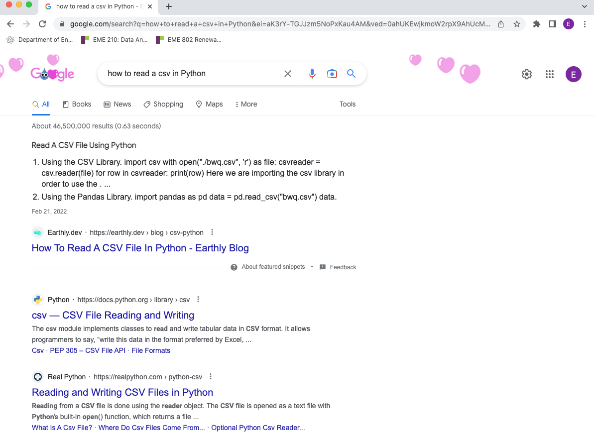
1. Google
With the appropriate search text, usually Google will return helpful information in the top three hits. You can search how to do something (e.g., "how to read a csv in Python"), and typically many tutorials will show up. Alternatively, if you get an error message in Python, you can try copying and pasting the message (or the key part of the message) in Google to see if anyone else has encountered this error (often someone has) and how they solved it.
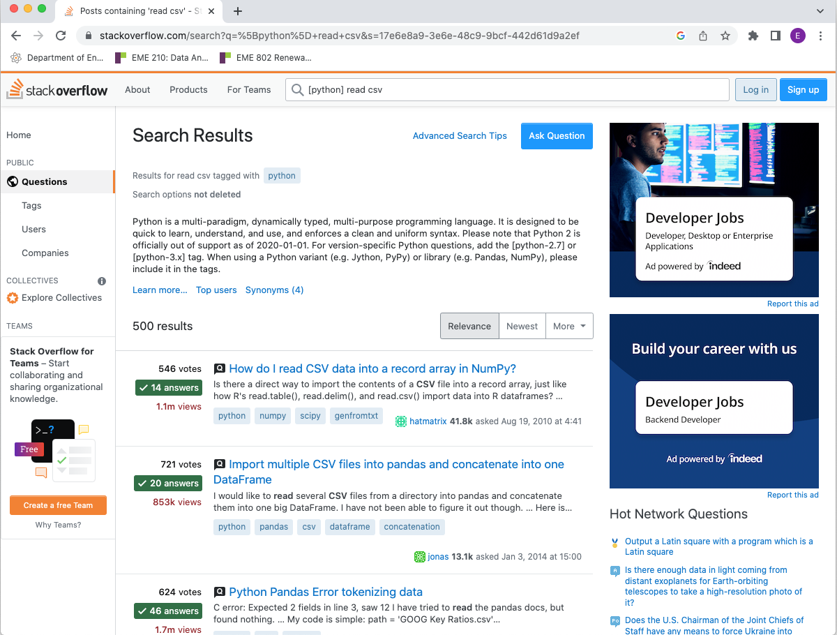
2. Stack Overflow
Stack Overflow [11] provides forums and discussions for anything related to coding (not just in Python). You can search for instructions or error diagnoses, and if you can't find what you are looking for, you can post your own question that others in the community can help you with. It is bad practice to post a question that has already been answered, so don't be surprised if you get rude responses if you do this!
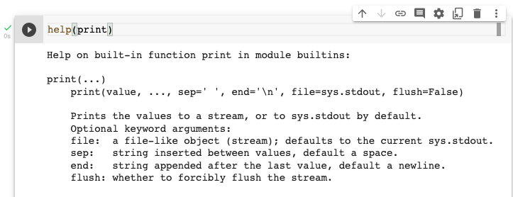
3. The help function in Python
In a Code Cell, typing and executing: help(function_name), will return some pared-down documentation of the function, including what the function does and what arguments/parameters it takes (along with default values, if any). Interpreting this sort of help is also discussed in the last part of the previous section [12], 6.) The basics of functions in Python.
4. The library documentation
You can also get detailed information on functions, constants, types, and other elements through online documentation. Any features that are natively built-in to Python are described in the Python Standard Library documentation [13]. Functions contained in imported libraries are described in that library's documentation (for example, Pandas [14]). In Python, a "library" is a collection of code, including functions, classes, and variables, among other things.
De-Bugging Code
The following video demonstrates each of these four approaches to getting help with Python:
Python Coding Fundamentals: Libraries
Libraries
In Python, a “library” is a collection of code, including functions, classes, and variables, among other things. The way that Python works is that you have different libraries that contain different sets of functions, and you use the functions in any given library once you load the library into your session. There are some base functions within Python that you can use without loading any libraries, but a lot of the more complex data analysis tasks in this class are going to require the use of libraries. Each library in Python has a documentation website, and each library's documentation will be in a similar format to other libraries. The links below take you to the documentation for most of the libraries we'll use in this course, and subsequent lessons will instruct you on the use of many of the functions contained in these libraries. Most of the libraries will have something called examples or tutorials. Some libraries may also have galleries. But, essentially, these documentation sites will have resources that you can use to build if you need an example or need to figure out how something works or even just to figure out how to customize something or see what the options are for a certain command.
The main libraries used in this course are:
NumPy | NumPy User Guide [15]
NumPy is a very popular and almost necessary library within Python called NumPy. This library is used to do mathematics with arrays, vectors and other numerical routines. If you wanted to calculate 2 + 2, for example, you could do that in Python. But if you want to do an array, 2, 2, + another array, 4, 4, and get ultimately what would be 6, 6, you need the NumPy array to do that more complex math.
Pandas | Pandas User Guide [16]
Another package that we'll be using quite a bit in this class is called Pandas. And this is really great fto use when working with complex data sets. Pandas it works with something that we'll discuss later called a DataFrame, which is akin to a table in Excel. In fact, a lot of the functionality of Pandas is similar to that of Excel. You can call with columns. You can call rows. You can do complex math. You can sort, filter, et cetera.
Matplotlib | Matplotlb User Guide [17]
Matplotlib is a very popular package used for visualizing data and making plots, and uses MATLAB-like syntax.
Seaborn | Seaboorn User Guide [18]
Seaborn is a more advanced plotting tool that's used in a lot of statistical purposes, but can be a little bit rigid in some cases when you try to add different elements to the plot.
Plotnine | Plotnine User Guide [19].
Plotnine is what is referred to as the Grammar of Graphics visualization library. This means that it operates similar to how one would construct a sentence, adding prepositions and additional verbs and nouns. For example, in a sentence, you could start with "The quick...". Then, if you wanted to extend the sentence, you could say "The quick brown fox...". You could go further and add a verb: "The quick brown fox jumps...", and so forth, continuing to add on words that ultimately keep extending the sentence with new information. Plotnine works in a similar way where, for example, one starts with a bar plot, and then adds error bars, and then text labels, and so on, building complex plots from individual elements.
Because Python is open source, there are a lot of opportunities online to find snippets of code. You are more than welcome to find an example that's close to what you're trying to do, and then modify it to work for your intended purpose. That's often how a lot of code gets built, especially at the beginning when trying to figure out how different functions operate and how to accomplish certain tasks in Python.
Take a Minute
Take a minute to explore the links to the libraries listed above.
Data Structures
Data Structures
With this being a data analytics course, it is important to start with a focus on data. Data comes in a lot of different forms and can be organized into many different structures. The list below covers some main, basic data structures, in general terms:
Scalar
A scalar is just a single value. For example:
Vector
A vector contains multiple scalars organized into a single row:
or column:
The defining feature of a vector is that it is one-dimensional, regardless of which direction it goes.
Matrix
A matrix contains multiple values organized into a 2-dimensional array:
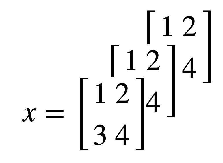
Tensor
A tensor is a multidimensional set of arrays. For example, a 3-dimensional tensor can be thought of as a stack of matrices:
Table
So far, all the data structures listed above are for a single data type (i.e., only numbers). A table contains multiple variables (or vectors) organized into columns, and the different variables can have different data types (e.g., numbers and text), although any single variable needs to contain only a single data type (we'll talk more about data types in Lesson 2). Furthermore, tables typically have labels for the variables, as column headings:
| HOME ID | DIVISION | KWH |
|---|---|---|
| 10460 | Pacific | 3491.900 |
| 10787 | East North Central | 6195.942 |
| 11055 | Mountain North | 6976.000 |
| 14870 | Pacific | 10979.658 |
| 12200 | Mountain South | 19472.628 |
| 12228 | South Atlantic | 23645.160 |
| 10934 | East South Central | 19123.754 |
| 10731 | Middle Atlantic | 3982.231 |
| 13623 | East North Central | 9457.710 |
| 12524 | Pacific | 15199.859 |
* Data Source: Residential Energy Consumption Survey (RECS) [20], U.S. Energy Information Administration (accessed Nov. 15th, 2021)
 Assess It: Check Your Knowledge
Knowledge Check
Data Structures: Pandas
Data Structures: Pandas
The previous page discussed data structures in general, using common terminology. Here, we focus on two data structures common to the Pandas library:
1. Series
There is a specific data structure in the Pandas called a series. This is very similar to a vector because it is in one-dimensional, but the key difference is that a series is labeled. For an example, run the following code:
So, the numbers 1-5 are our data in this example, whereas a-e, defined in the parameter “index”, are our indices or labels. These labels are handy for retrieving specific values out of the Series; try adding print(s['c']) to the above code and see what happens. This should return the value 3 for you.
If we didn't supply the “index” parameter, the default is to number the indices with sequential integers starting at 0.
2. DataFrame
Similarly, Pandas also has a table-style data structure, called a “DataFrame”. Typically, a DataFrame will have column labels (the same as the headings in a table, and these are treated effectively as variable names), and also row labels or indices (think of these as row numbers). So, for example, if we want to coerce the table from the previous page into a Pandas DataFrame:
Note that the first variable, HOME ID, is entered as an array (values separated by commas and encased in [ ]), whereas the other two variables are entered as Series. This is just to show some of the various ways you can enter data. Furthermore, as with the Series function, we can customize our row indices by supplying an “index” parameter to the DataFrame fuction.
Throughout this course, we'll be working a lot with DataFrames. This will be our default structure for datasets. The next few pages will show you how to import data into a DataFrame object in Python. In Lesson 2, we will cover some common tools for manipulating data into a DataFrame. It is critical to feel comfortable with DataFrames, as they are an incredibly useful way to store data and essential for any Pandas-based data analytics.
Importing Files: Option 1
Importing Files: Option 1
 Read It: Importing Files
Introducing Comma Separated Value files
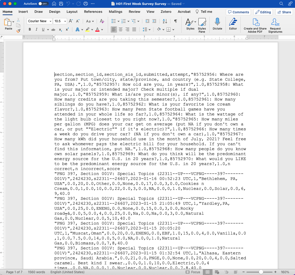
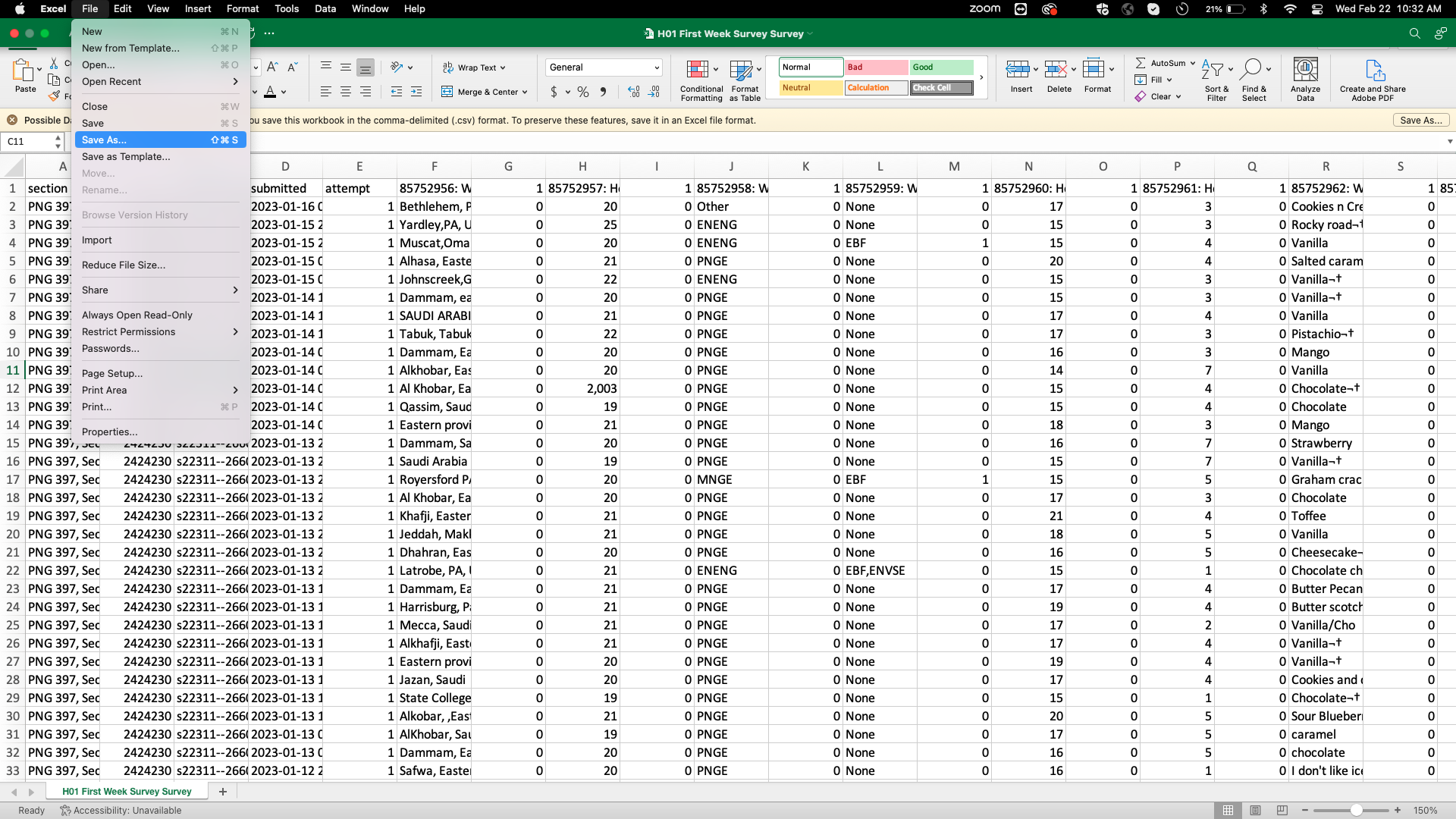
In this course, you will primarily work with CSV (comma-separated value) files. You can recognize these files in your computer file system as xxxxxxx.csv files, with the “.csv” extension. These files can be easily opened with spreadsheet software, such as Microsoft Excel or Google Sheets. Technically, they can even be opened by Microsoft Word or basic text editors. However, they may not look like a table in those formats! Below we have some examples of what a CSV file looks like in Excel, Word, and a generic text editor.


CSV files are also easy to read into nearly every programming language. This means that if you're working in Python, you can read in a CSV file, make some changes, write to a new CSV file, and send the new file to a colleague working in R or MATLAB. If it is in CSV format, they will be able to open the same file and see what you did without any issues going between the languages.
How to read files into Google Colab
When you are using Python, you can read other file types beyond CSV files. For example, Python can read an Excel spreadsheet (“.xls” or “.xlsx” extensions) or a text file (“.txt” extension). If you get into more advanced coding, you can read in GIS files or Google Maps files. In Python, you can read nearly any file type that you come across, but in this class, we'll be using CSV files.
Occasionally, you may come across data that is in Excel format (“.xlsx” extension), but want to read it into Python as a CSV file. In this case, you can easily convert your file using the “Save As...” feature, shown below.

Once you have your data in CSV format, you need to upload that data to Colab. To do this, we will be using the Pandas library [14], which was introduced previously in this lesson. In this lesson, we will be demonstrating three main ways to import CSV files into Colab, the first of which uses your existing Google Drive. Note that in order to use this method of uploading files, you will need to have your CSV file of interest stored on your Google Drive prior to running the code.
 Watch It: Video - Importing Files: Option1 (5:44 minutes)
 Try It: Apply Your Coding Skills in Google Colab
- The Google Colab file used in the video is linked here [21].
- Go to the Colab file and click “File” then “Save a copy in Drive”, this will create a new Colab file that you can edit in your own Google Drive account.
- Once you have it saved in your Drive, try to implement the following code to import a file of your choice by mounting your Google Drive:
Note: You must be logged into your PSU Google Workspace in order to access the file.
1 2 3 4 5 6 7 8 9 | from google.colab import drivedrive.mount('/content/drive')import pandas as pddf = pd.read_csv('yourfilename.csv')df # print the dataframe |
Once you have implemented this code on your own, come back to this page to test your knowledge.
Assess It: Check Your Knowledge
Knowledge Check
Importing Files: Option 2
Importing Files: Option 2
Read It: Importing Files
Here, we are continuing to explore means in which we can read CSV files into Google Colab. Here, we will use the "drag and drop" method. This does not require you to have your files stored on Google Drive, such as the previous example, but instead can be stored anywhere on your local computer.
Watch It: Video - Importing Files: Option 2 (3:03 minutes)
Try It: Apply Your Coding Skills in Google Colab
- The Google Colab file used in the video is linked here [22].
- Go to the Colab file and click "File" then "Save a copy in Drive", this will create a new Colab file that you can edit in your own Google Drive account.
- Once you have it saved in your Drive, try to implement the following code to import a file of your choice by mounting your Google Drive:
Note: You must be logged into your PSU Google Workspace in order to access the file.
1 2 3 | import pandas as pddf = pd.read_csv('yourfilename.csv') |
Once you have implemented this code on your own, come back to this page to test your knowledge.
Assess It: Check Your Knowledge
Knowledge Check
FAQ
Importing Files: Option 3
Importing Files: Option 3
Read It: Importing Files
The final demonstration for reading in CSV files is the "Upload Files" method. Similar to the "Drag and Drop" method, this method also requires your CSV file be stored somewhere on your local computer. However, instead of manually moving the file into the Google Colab space, as previously shown, we are going to create a special "upload" button which will be able to connect to your local computer. This method does involve a new library, namely the IO library [23], which will allow you to move between Google's cloud-based memory space and your individual Google Colab file space.
Watch It: Video - Importing Files: Option 3 (5:47 minutes)
Try It: Apply Your Coding Skills in Google Colab
- Click the Google Colab file used in the video is linked here [24].
- Go to the Colab file and click "File" then "Save a copy in Drive", this will create a new Colab file that you can edit in your own Google Drive account.
- Once you have it saved in your Drive, try to implement the following code to import a file of your choice by mounting your Google Drive:
Note that you must be logged into your PSU Google Workspace in order to access the file.
1 2 3 4 5 6 7 8 9 | from google.colab import filesuploaded = files.upload()import ioimport pandas as pddf = pd.read_csv(io.BytesIO(uploaded['yourfilename.csv'])) |
Once you have implemented this code on your own, come back to this page to test your knowledge.
Assess It: Check Your Knowledge
Knowledge Check
FAQ
Dictionaries vs. DataFrames
Dictionaries vs. DataFrames
Read It: Dictionaries vs. Dataframes
So far in this lesson, we have been primarily working with DataFrames. However, there is another common data structure in Python: dictionaries. Dictionaries can be used with "Base Python", so there is no need to import any additional libraries, but they do not have the same functionality as DataFrames. In the coding demonstration below, we will demonstrate how to create a dictionary and how to convert dictionaries into DataFrames.
Watch It: Video - Dictionaries vs. DataFrames (5:57 minutes)
Try It: DataCamp - Apply Your Coding Skills
Dictionaries are a quick way to create a variable from scratch. However, their functionality is limited, so we will often want to convert those dictionaries into DataFrames. Try to code this conversion in the cell below. Hint: Make sure to import the Pandas library.
Assess It: Check Your Knowledge
Knowledge Check
Summary and Final Tasks
Summary
In Lesson 1, you've now gotten a sense of what we are referring to with the word "data", and the different forms and structures in which data can typically be stored. Importantly, you can now start coding in Python in Google Colab, which will be critical for the homework assignments. Also, important is importing data with Python, and in Lesson 1 you have been presented with a number of ways of accomplishing that.
Assess it: Check Your Knowledge Quiz
Reminder - Complete all of the Lesson 1 tasks!
You have reached the end of Lesson 1! Double-check the to-do list on the Lesson 1 Overview page to make sure you have completed all of the activities listed there before you begin Lesson 2.