Lesson 4: Confidence intervals and bootstrapping
Overview
Overview
A critical step in making statistical inferences from a sample is defining how confident you are in those results. In this lesson, we will introduce sampling distributions, bootstrapping, and confidence intervals to provide this measure of confidence. You will learn how to create a sampling distribution from bootstrapping, as well as how to use that bootstrapped sampling distribution to determine the confidence interval. In particular, we will focus on two key methods for calculating confidence intervals: the standard error method and the percentile method.
Learning Outcomes
By the end of this lesson, you should be able to:
-
define a confidence interval for a dataset
-
draw conclusions from a confidence interval
-
estimate a confidence interval using bootstrapping
Lesson Roadmap
| Type | Assignment | Location |
|---|---|---|
| To Read | Lock, et al. 3.1-3.4 | Textbook |
| To Do |
Complete Homework: H05 Confidence Intervals Take Quiz 4 |
Canvas Canvas |
Questions?
If you prefer to use email:
If you have any questions, please send a message through Canvas. We will check daily to respond. If your question is one that is relevant to the entire class, we may respond to the entire class rather than individually.
If you prefer to use the discussion forums:
If you have questions, please feel free to post them to the General Questions and Discussion forum in Canvas. While you are there, feel free to post your own responses if you, too, are able to help a classmate.
Sampling Distributions
 Read It: Sampling Distributions
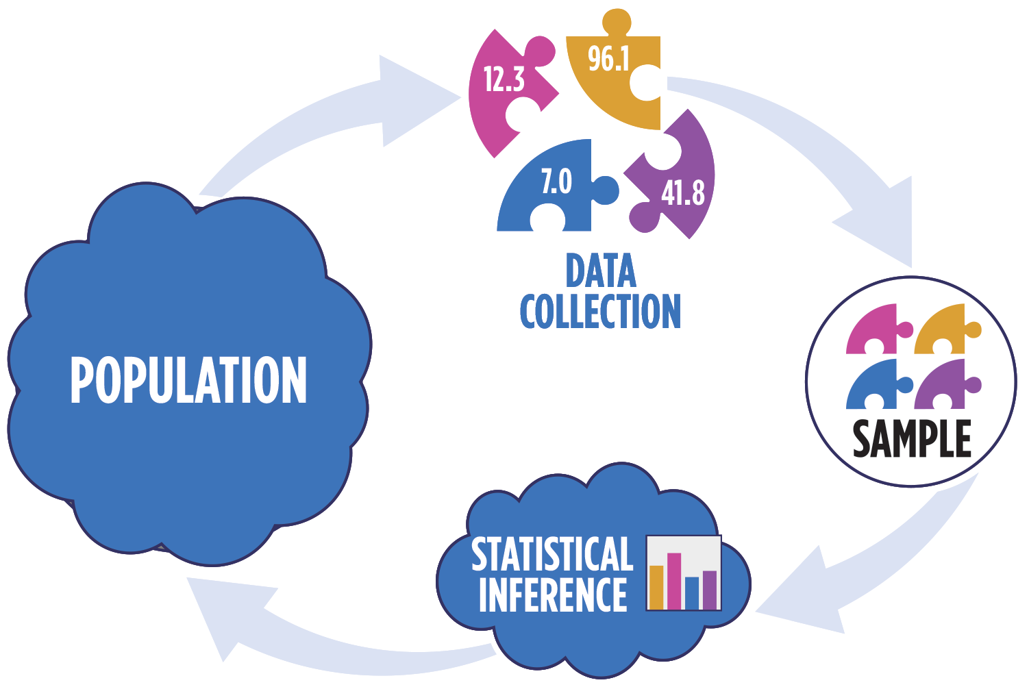
Recall the animation from Lesson 1, showing the process of collecting a sample from a population, then using that sample to make an inference about the population.
Often, we will want to collect a number of samples in order to bolster the statistical power of our inference. In other words, we want to obtain a sampling distribution, which we can use to conduct statistical inference tests. This sampling distribution is made up of some statistic (e.g., the mean) of each individual sample. For example, say we roll two dice 10 times and record the average roll, this average is . Then, we repeat the process with a new set of 10 rolls, and so on, until we have a large number of samples. Each of these individual s makes up the sampling distribution, which can be visualized in the figure below.
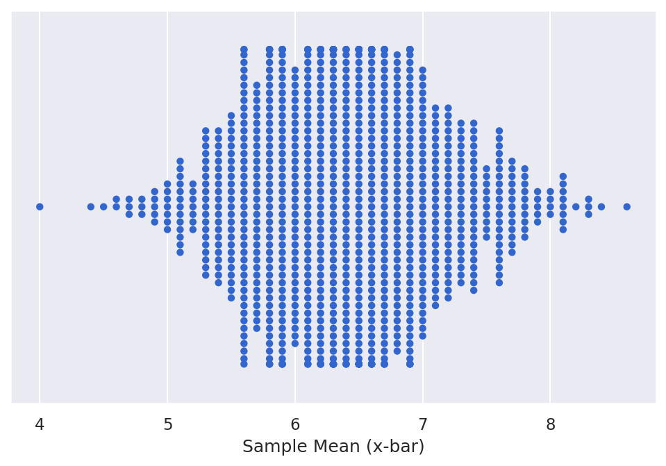
In this figure, each point represents the statistic (e.g., , ). Note that for most parameters, the sampling distribution will be centered at the population parameter if the following are met:
- The samples are random
- The sample size is large enough
- There are enough samples
Definition: The sampling distribution is the distribution of sample statistics (e.g., , ) calculated on different samples of the same size and from the same population.
 Watch It: Video - Introduction to Sampling Distributions (10:33 minutes)
Watch It: Video - Comparing Samples to Population (13:51 minutes)
 Try It: Apply Your Coding Skills in Google Colab
- Click the Google Colab file used in the video is linked here. [2]
- Go to the Colab file and click "File" then "Save a copy in Drive", this will create a new Colab file that you can edit in your own Google Drive account.
- Once you have it saved in your Drive, use the partial code below to add two additional samples to the dataframe with data from 10 dices rolls each (use either real dice or a virtual roller [3]), then calculate the new sample distribution.
Note: You must be logged into your PSU Google Workspace in order to access the file.
1 2 3 4 5 6 7 8 9 10 11 12 13 14 15 | # Dice roll data, as data framedata_df = pd.DataFrame({'sample1' : [5, 7, 4, 6, 3, 8, 7, 7, 8, 6], 'sample2' : [3, 11, 7, 9, 7, 2, 7, 5, 4, 8], 'sample3' : [7, 8, 6, 10, 8, 4, 9, 3, 9, 11], 'sample4' : [5, 6, 6, 6, 4, 7, 6, 7, 3, 7], 'sample5' : [...], 'sample6' : [...})# melting the data to get it into "long form"data_df = data_df.melt(value_vars = [...], var_name = 'Sample', value_name = 'Outcome')# Find the mean of each sampledata_means = ...data_means |
 Assess It: Check Your Knowledge
Knowledge Check
 FAQ
FAQ
Standard Deviation and Standard Error
Read It: Standard Deviation and Standard Error
When working with sampling distributions, we distinguish the standard deviation from the standard error. Both measures are calculated the same way (e.g., through the typical standard deviation formula), the difference is the type of data they are applied to. The standard deviation is applied to the actual data (sample or population) and is a measure of the variance from the mean. The standard error is applied to the sampling distribution and is a measure of the variance from the true population parameter. The video below will show the difference in calculating these measures in Python.
Watch It: Video - Standard Deviation and Standard Error (03:26 minutes)
Assess It: Check Your Knowledge
Knowledge Check
FAQ
Add new questions
Introduction to For Loops
Read It: For Loops
For loops can be used to perform calculations and store variables iteratively. In Python, there are several keywords that all for loops must have:
-
for --- This command starts the for loop
-
in --- This command sets the number of iterations
-
: --- This command says that everything that follows is meant to be executed in the loop (until the indentation changes)
Below, we demonstrate the basics of for loops.
Watch It: Video - Introduction to For Loops (07:15 minutes)
Try It: DataCamp - Apply Your Coding Skills
Try to implement a simple for loop below. You want to iterate the loop 5 times, each time printing the index number.
Assess It: Check Your Knowledge
Knowledge Check
FAQ
Bootstrapping
Read It: Bootstrapping
Recall from the Sampling Distribution lesson that sampling distributions need to be sufficiently large in order to be considered representative of the population. However, this is often difficult to get, as sampling distributions often contain upwards of 1000 samples. Remember how you rolled two dice 10 times, recording the total value each time? Imagine doing that 1000 times in order to collect a larger enough sampling distribution! To avoid this arduous process, we use bootstrapping.
Bootstrapping, as demonstrated above, allows us to approximate the sampling distribution through resampling the initial sample. In other words, we randomly select values from the original sample with replacement over many iterations to develop a bootstrapped sampling distribution. The process is outlined below.
When we implement bootstrapping in code, we will leverage for loops that follow this basic pseudo-code process:
-
Obtain a sample of size n
-
For i in 1, 2, ..., N
-
Randomly draw n values from the original sample, with replacement
-
Store these values in the ith row of the bootstrap sample
-
Calculate the statistic of interest for the ith bootstrap sample
-
Store this value as the ith bootstrap statistic
-
-
Combine all N bootstrap statistics into the bootstrap sampling distribution
Watch It: Video - Introduction to Bootstrapping (11:29 minutes)
Try It: Apply Your Coding Skills in Google Colab
- Click the Google Colab file used in the video here. [4]
- Go to the Colab file and click "File" then "Save a copy in Drive", this will create a new Colab file that you can edit in your own Google Drive account.
- Once you have it saved in your Drive, use the partial code below to implement a bootstrapping procedure.
Note: You must be logged into your PSU Google Workspace in order to access the file.
1 2 3 4 5 6 7 8 9 10 11 12 13 14 15 16 | # STEP 1: initialize variablesN = ... # insert a sufficiently large iteration valuen = 10 # sample size = 10# empty dataframe:boot_df = pd.DataFrame({'sample': [np.nan] * (N*n), 'outcome': [np.nan] * (N*n), 'type': [np.nan] * (N*n)})# implement the bootstrapping procedure:for i in range(...): low_i = n*i high_i = low_i + (n-1) boot_df.loc[low_i:high_i, 'outcome'] = np.random.choice(..., ..., ...) boot_df.loc[low_i:high_i, 'sample'] = 'boot' + str(i+1) boot_df.loc[low_i:high_i, 'type'] = 'bootstrap' |
Assess It: Check Your Knowledge
Knowledge Check
FAQ
Bootstrapped Sampling Distributions
Read It: Bootstrapped Sampling Distributions
Once we have the bootstrapped samples, we need to calculate the sampling distribution, which contains the statistic of each sample. Below we demonstrate this process.
Watch It: Video - Bootstrapped Sampling Distributions (07:52 minutes)
Try It: Apply Your Coding Skills in Google Colab
- Click the Google Colab file used in the video here [5].
- Go to the Colab file and click "File" then "Save a copy in Drive", this will create a new Colab file that you can edit in your own Google Drive account.
- Once you have it saved in your Drive, use the partial code below to calculate and plot the bootstrapped sampling distribution. Alternatively, you can continue to edit your Colab file from the previous module.
Note: You must be logged into your PSU Google Workspace in order to access the file.
1 2 3 4 5 | # Find the mean of each sampleboot_means = ...# plot(ggplot(...) + geom_dotplot(...)) |
Assess It: Check Your Knowledge
Knowledge Check
FAQ
(add new questions)
Introduction to Confidence Intervals
Read It: Confidence Intervals
When we start making statistical inferences, we need means to represent the uncertainty in the results or the confidence that we, as the analysts, have in those results. For this, we turn to confidence intervals.
Definition: A confidence interval is an interval, computed from a sample, that has a predetermined change of capturing the value of the population parameter
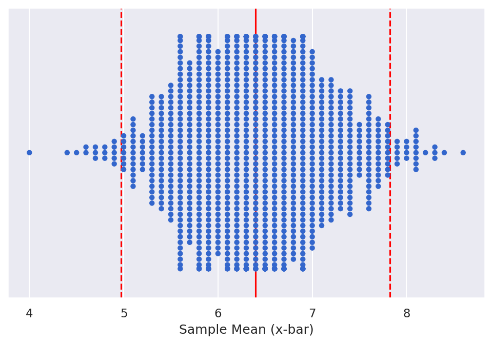
There are some key aspects here that we can further define. The first is that confidence intervals are computed from a sample. Therefore, we are not computing confidence intervals on the population, but using the sample or sampling distribution. The next aspect is the emphasis on predetermined chance. This refers to the confidence level that you are using in your analysis. Essentially, this level specifies how confident are you that the true population parameter falls within a certain range. Often, you will see the 95th, or 95%, confidence interval, which is the most common interval to use. An example of this 95% confidence interval is shown below.

In the upcoming videos, we will demonstrate two methods for using bootstrapped sampling distributions to determine the 95% confidence interval.
Assess It: Check Your Knowledge
Knowledge Check
FAQ
(add new questions)
Confidence Intervals: The Percentile Method
Read It: Confidence Intervals: The Percentile Method
For some confidence intervals, there is no easy standard error equation. In these situations, we can use the percentile method to estimate the confidence interval. In this method, we assume that the data is normally distributed so that the confidence interval can be represented by the percentage of data outside the interval. For example, with the 95% confidence interval, we can use the percentile method to say that the lower bound is at the 2.5% mark and the upper bound is at the 97.5% mark, with 95% of the data in between. To calculate this, we follow these steps:
- 100 - 95 = 5
- 5/2 = 2.5
- Lower Bound: 0 + 2.5 = 2.5
- Upper Bound: 100 - 2.5 = 97.5
- Thus, the CI is: [quantile(0.025), quantile(0.975)
This is demonstrated below.
Watch It: Video - Introduction to Sampling Distributions (07:11 minutes)
Try It: Apply Your Coding Skills in Google Colab
- Click the Google Colab file used in the video is here. [6]
- Go to the Colab file and click "File" then "Save a copy in Drive", this will create a new Colab file that you can edit in your own Google Drive account.
- Once you have it saved in your Drive, use the partial code below to calculate the 95% confidence interval using the percentile method.
Note: You must be logged into your PSU Google Workspace in order to access the file.
1 2 3 4 5 6 7 | # step 1: calculate lower percentile (this is the lower bound of the CI)LP = ...# step 2: calculate the upper percentile (this is the upper bound of the CI)UP = ...print('the 95% confidence interval is ', ...) |
Assess It: Check Your Knowledge
Knowledge Check
FAQ
Confidence Intervals: The Standard Error Method
Read It: Confidence Intervals: The Standard Error Method
To determine the 95% confidence interval through the standard error method, we use the following equation
This equation centers the confidence interval around the sampling distribution mean (""), as shown in the figure below.
In order to calculate this, we take three key steps in the code, following the development of the bootstrapped sampling distribution.
- Calculate the mean of the bootstrapped sampling distribution using
- Calculate the standard error of the bootstrapped sampling distribution using
- Calculate the 95% confidence interval using the equation above
Below we demonstrate this process.
Watch It: Video - Introduction to Sampling Distributions (07:12 minutes)
Watch It: Video - Confidence Intervals SEmethod (04:58 minutes)
Try It: Apply Your Coding Skills in Google Colab
- Click the Google Colab file used in the video here. [7]
- Go to the Colab file and click "File" then "Save a copy in Drive", this will create a new Colab file that you can edit in your own Google Drive account.
- Once you have it saved in your Drive, use the partial code below to calculate and plot the 95% confidence interval.
Note: You must be logged into your PSU Google Workspace in order to access the file.
1 2 3 4 5 6 7 8 9 10 11 12 13 14 15 | # step 1: calculate x barXB = ...# step 2: calculate the standard errorSE = ...# step 3: calculate the 95% Confidence IntervalCI = ...(ggplot(boot_means) + geom_dotplot(...) + geom_vline(aes(xintercept = 7), color = 'blue', size = 1) + geom_errorbarh(...) + geom_point(...)) |
Assess It: Check Your Knowledge
Knowledge Check
FAQ
(add new questions)
Summary and Final Tasks
Summary
Through this lesson, you are now able to define a confidence interval and calculate the interval using bootstrapped sampling distributions. You also learned how to create for loops, which we will continue to use throughout the course.
Assess It: Check Your Knowledge Quiz
Reminder - Complete all of the Lesson 4 tasks!
You have reached the end of Lesson 4! Double-check the to-do list on the Lesson 4 Overview page to make sure you have completed all of the activities listed there before you begin Lesson 5.