Lesson 6: Normal distribution and Central Limit Theorem
Overview
Overview
In the previous two lessons, you have learned how to implement confidence intervals and hypothesis tests using randomization procedures. In this lesson, we will return to these ideas, but introduce the "traditional" ways to conduct these tests through the central limit theorem. Additionally, we will discuss the one-line tests that can be used to quickly implement a hypothesis test on a given dataset. You will learn about the central limit theorem and its role in traditional statistical inference, as well as how and when to implement the one-line hypothesis tests.
Learning Outcomes
By the end of this lesson, you should be able to:
-
differentiate between the Normal vs. t-Distrbution
-
express the relationship between these distributions to confidence intervals and hypothesis tests
-
recall the Central Limit Theorem
-
test hypotheses with pre-made Python functions
Lesson Roadmap
| Type | Assignment | Location |
|---|---|---|
| To Read | Lock et. al. 5.1, 5.2, & 6 | Text book |
| To Do |
Complete homework: H08 Even More Hypothesis Testing |
Canvas |
Questions?
If you prefer to use email:
If you have any questions, please send a message through Canvas. We will check daily to respond. If your question is one that is relevant to the entire class, we may respond to the entire class rather than individually.
If you prefer to use the discussion forums:
If you have questions, please feel free to post them to the General Questions and Discussion forum in Canvas. While you are there, feel free to post your own responses if you, too, are able to help a classmate.
Normal Distribution and Z-Scores
Normal Distribution and Z-Scores
 Read It: The Normal Distribution
The normal distribution is a common distribution of data, which is frequently plotted as a bell-shaped curve. In this curve, the mean is plotted at the center or peak of the bell with the sides of the curve being completely symmetrical. The width of this curve is determined by the standard deviation of the data. In this sense, to plot a normal distribution, you need only two parameters: the mean and the standard deviation. We define, or denote, the normal distribution by using the capital letter N, followed by the mean, μ, and the standard deviation, σ. You can calculate the normal distribution for any any dataset using the probability distribution function, shown below.
The probability density function (pdf) of the Normal distribution is:
with parameters = mean and = standard deviation
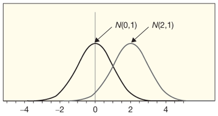
The standardized version of normal distribution has a mean of 0 and a standard deviation of 1, as shown in the figure below. Note that by changing the mean from 0 to 2, the plot shifts to the right, but maintains the same width since we did not change the standard deviation.

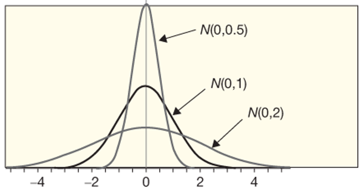
In the figure below, you can see as the standard deviation goes from 0.5 to 2, the curves get wider, but the plot remains centered at 0 since we do not change the mean at all.

 Read It: Z-Scores
Often, when working with traditional statistical inference, you will need to calculate a quantity known as the "z-score". The z-score is a means of standardizing any data to fit with the standard normal distribution (e.g., N(0,1)). This calculation is performed using the equation below. Essentially, you subtract the mean from your data and divide by the standard deviation.
Traditionally, this z-score is used to find confidence intervals and test hypotheses using the central limit theorem. However, it can also be used to detect outliers: a z-score > 3 is generally considered to be an outlier.
 Watch It: Fitting Normal Distributions - (7:45 minutes)
 Try It: Google Colab
- Click the Google Colab file used in the video here [2].
- Go to the Colab file and click "File" then "Save a copy in Drive", this will create a new Colab file that you can edit in your own Google Drive account.
- Once you have it saved in your Drive, try to edit the following code to fit a normal distribution to some data:
Note: You must be logged into your PSU Google Workspace in order to access the file.
1 2 3 4 5 6 7 8 9 10 | meandist = ...SEdist = ...phatdf['x_pdf'] = np.linspace(...) phatdf['y_pdf'] = stats.norm.pdf(..., loc = ..., scale = ...)(ggplot(...) + geom_dotplot(aes(...), dotsize = 0.25) + geom_line(aes(...), color = 'red', size = 1)) |
Once you have implemented this code on your own, come back to this page to test your knowledge.
 Assess It: Check Your Knowledge
Knowledge Check
Central Limit Theorem
Central Limit Theorem
 Read It: The Central Limit Theorem
In the previous page, we discussed the normal distribution and z-scores. The reason we are able to use the normal distribution and z-scores to find confidence intervals and conduct hypothesis tests is called the Central Limit Theorem. This statistical theory provides evidence for normally distributed sampling distributions, even if the original data are not normally distributed.
Provided a sufficiently large sample size and identically distributed independent samples, the central limit theorem finds that the standardized sample means tend towards the standard normal distribution.
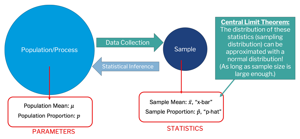
In other words, if our sample size is large enough, the sampling distribution should tend toward normal. This is why our randomization procedures often lead to bell-shaped histograms when showing the sampling distribution. The central limit theorem is also why we can make statistical inferences about a population even though we only collect a sample of the data, as shown in the image below. In other words, say you collect some data, this is your sample, which has some statistics (e.g., , , etc.). The central limit theorem tells us that the distribution of these sample statistics can be approximated with a normal distribution, assuming that the sample size is sufficiently large enough.
An important question, however, is what is "sufficiently large"? It is a little subjective, and it often depends on your data. In chapter 3 of the textbook, the authors provide an example of how to calculate the optimal sample size to meet the criteria for the central limit theorem. However, for most of this class, we will aim for at least 1,000 values in our sampling distributions. Note, this is the "N" in our randomization procedures! We also want to maintain a large enough sample from which we are randomly drawing values (the "n" in the randomization procedures). Generally, you will want at least 30 or 50 data points to ensure that you have a large enough of pool of data to draw from.

 Assess It: Check Your Knowledge
Knowledge Check
Confidence Intervals and the Central Limit Theorem
Confidence Intervals and the Central Limit Theorem
 Read It: Confidence Intervals and the Central Limit Theorem
One application of the central limit theorem is finding confidence intervals. To do this, you need to use the following equation. Note that the z* value is not the same as the z-score described earlier, which was used to standardize the normal distribution. Here, the confidence interval is the sample statistic (e.g., , , etc.) plus/minus the z* value times the standard error. Note that this is the same equation we used in Lesson 4 when you learned about the standard error method. In Lesson 4, the z* value was set to 2 for the 95% confidence interval. This was an approximation of the z* value, which is actually 1.96 for an alpha value of 0.05.
where z* is chosen so that %P of the distribution is between -z* and +z* for %P confidence level.
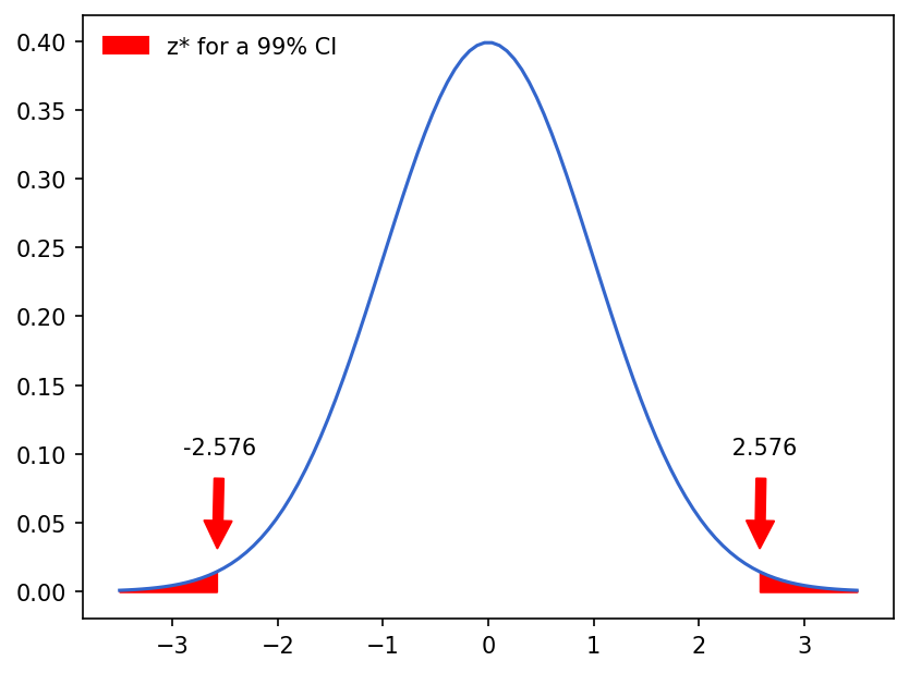
The z* value, therefore, is only dependent on the confidence level. In other words, if you consider two very different datasets, the sample statistic and standard error will change, but the z* value will remain the same as long as you are using the same confidence level for both datasets. These z* values can be found in tables that list the values for a given alpha level, making it easy to quickly find different confidence intervals for the different levels. For example, for a 99% confidence interval, shown below, the z* value is 2.576. The confidence interval could then be calculated by plugging that value into the above equation, along with the sample statistic and standard error.

Example of a 99% confidence interval calculated using the z* value.
 Watch It: Video - Confidence Interval from Normal Distribution (5:32 minutes)
 Try It: DataCamp - Apply Your Coding Skills
Try to find the 99% confidence interval of the 'phatdf' dataframe using the z* method discussed above.
 Assess It: Check Your Knowledge
Knowledge Check
Hypothesis Tests and the Central Limit Theorem
Hypothesis Tests and the Central Limit Theorem
 Read It: Hypothesis Tests and the Central Limit Theorem
Similar to calculating confidence intervals, you can also use the z-score to conduct hypothesis tests. In particular, you need to calculate a new statistic, often referred to as the "z statistic", that requires the sample statistic (e.g., ), null parameter, and standard error. Therefore, unlike the z* value for the confidence intervals, the z-statistic is wholly dependent on the data and the hypothesis test that you are conducting and will need to be recalculated for every new test you conduct. The equation for the z-statistic is shown below.
In order to obtain a conclusion from a hypothesis test, we need to find the p-value. If you are following the traditional method, the p-value is calculated as the proportion of the standard normal distribution that is at least as extreme as the z-statistic, as shown below.

 Watch It: Video - Calculating P-Values Using the Normal Distribution (5:06 minutes)
 Try It: DataCamp - Apply Your Coding Skills
Try to find the left and right tailed p-value of the proportion dataset using the z-statistic method discussed above. The null hypothesis is:
Ho: ρ = 0.5
 Assess It: Check Your Knowledge
Knowledge Check
Student's t-Distribution
Student's t-Distribution
 Read It: Student's t-Distribution
Recall that the central limit theorem only applies for "sufficiently large" sample sizes. Often, you may encounter smaller datasets for which the central limit theorem doesn't apply. In those situations, we use an approximation known as the Student's t-Distribution. In this distribution, the shape is dependent on the degrees of freedom (i.e., the maximum amount of independent values), which is often calculated as the number of data points minus one, as shown below.
Ultimately, this results in a curve that is often shorter and wider than the standard normal, with smaller sample sizes resulting in larger differences. In other words, there are fewer data points close to the mean and more data points towards the outside. These changes are shown in the figure below.

Example of the Student's t-Distribution. Notice how the plot is becoming wider (e.g., more data on the outside) as the number of samples decreases.
 Assess It: Check Your Knowledge
Knowledge Check
Traditional Statistical Inference
Traditional Statistical Inference
 Read It: Summary of Traditional Statistical Inference
Recall from earlier in the lesson, you used the z* values and the z-statistics to calculate confidence intervals and p-values. You can also use those values to make conclusions from each of the hypothesis tests that we covered in Lesson 5. Below is a table that outlines how to fond the standard error, confidence interverals, and p-value for each of the hypothesis tests using the z-related formlas.

Download pdf: Summary of Types of Inference [3]
Significance
Significance
 Read It: Significance
So far in this course, we have been using various data samples, most of which are quite large (e.g., they have a large value for "n"). However, in real world applications, you might not have access to these large datasets. Imagine you are in a situation where it is too expensive or infeasible to collect more than a dozen data points. At this point, the sample size is likely not going to be considered "sufficiently large" and some of our tests will result in very different results. In the viedo below, we will walk through an experiement to see how the p-value changes with increasing sample size, leading to different conclusions.
 Watch It: Video - Significance (10:47 minutes)
 Try It: DataCamp - Apply Your Coding Skills
- Use this link to a card drawing simulator [4].
- Draw some cards to create your own x variable with card colors.
- Then, edit the code below to calculate the p-value.
- Try drawing different amounts of cards and see how the p-value changes.
Single Mean One-Line Test
Single Mean One-Line Test
 Read It: Single Mean One-Line Test
To conduct the one-line test for a single mean hypothesis test, you will use a one sample t-test. Below, we demonstrate how to implement this code.
 Watch It: Video - Hypothesis Test for Single Mean (5:45 minutes)
 Try It: Google Colab
- Click the Google Colab file used in the video here [5].
- Go to the Colab file and click "File" then "Save a copy in Drive", this will create a new Colab file that you can edit in your own Google Drive account.
- Once you have it saved in your Drive, try to edit the following code to run the single mean one-line test. Remember to import the libraries and run the code to create some data.
Note: You must be logged into your PSU Google Workspace in order to access the file.
1 2 3 4 5 6 7 8 9 10 | # Librariesimport numpy as npimport scipy.stats as stats# create some datax = np.random.randint(0,100,1000)# run one-line testresults = ...results.pvalue |
Once you have implemented this code on your own, come back to this page to test your knowledge.
 Assess It: Check Your Knowledge
Knowledge Check
 FAQ
FAQ
Single Proportion One-Line Test
Single Proportion One-Line Test
 Read It: Single Proportion One-Line Test
To conduct the one-line test for a single proportion hypothesis test, you will use a one sample binomial test. Below, we demonstrate how to implement this code.
 Watch It: Video - Single Proportion OneLine Test (3:54 minutes)
 Try It: Google Colab
- Click the Google Colab file used in the video here [6].
- Go to the Colab file and click "File" then "Save a copy in Drive", this will create a new Colab file that you can edit in your own Google Drive account.
- Once you have it saved in your Drive, ry to edit the following code to run the single proportion one-line test. Remember to import the libraries and run the code to create some data.
Note that you must be logged into your PSU Google Workspace in order to access the file.
1 2 3 4 5 6 7 8 9 10 11 12 13 14 15 | # Librariesimport numpy as npimport scipy.stats as stats# create some datax = np.random.randint(0,100,1000)# initialize the variablessuccess_rate = ... # success = the number of data points in x above 50samp_size = ... # sample size = the total number of data points in x# implement one-line testresults = ...results.pvalue |
Once you have implemented this code on your own, come back to this page to test your knowledge.
 Assess It: Check Your Knowledge
Knowledge Check
Difference of Means One-Line Test
Difference of Means One-Line Test
 Read It: Difference of Means One-Line Test
To conduct the one-line test for a two-sample difference of means hypothesis test, you will use a t-test for two independent samples. Below, we demonstrate how to implement this code.
 Watch It: Video - Paired Mean of Differences OneLine Test (2:03 minutes)
 Try It: Google Colab
- Click the Google Colab file used in the video here [7].
- Go to the Colab file and click "File" then "Save a copy in Drive", this will create a new Colab file that you can edit in your own Google Drive account.
- Once you have it saved in your Drive, try to edit the following code to run the difference of means one-line test. Remember to import the libraries and run the code to create some data.
Note: You must be logged into your PSU Google Workspace in order to access the file.
1 2 3 4 5 6 7 8 9 10 11 | # Librariesimport numpy as npimport scipy.stats as stats# create some datax = np.random.randint(0,100,1000)y = np.random.randint(0,200,1000)# implement one-line testresults = ...results.pvalue |
Once you have implemented this code on your own, come back to this page to test your knowledge.
 Assess It: Check Your Knowledge
Knowledge Check
Paired Mean of Differences One-Line Test
Paired Mean of Differences One-Line Test
 Read It: Paired Mean of Differences One-Line Test
To conduct the one-line test for a paired mean of differences hypothesis test, you will use a t-test for two related samples. Below, we demonstrate how to implement this code.
 Watch It: Video - Hypothesis Test for Two Samples: Mean of Differences (Paired Comparison) (2:03 minutes)
 Try It: Google Colab
- Click the Google Colab file used in the video here [8].
- Go to the Colab file and click "File" then "Save a copy in Drive", this will create a new Colab file that you can edit in your own Google Drive account.
- Once you have it saved in your Drive, try to edit the following code to run the paired mean of differences one-line test. Remember to import the libraries and run the code to create some data.
Note: You must be logged into your PSU Google Workspace in order to access the file.
1 2 3 4 5 6 7 8 9 10 11 | # Librariesimport numpy as npimport scipy.stats as stats# create some datax = np.random.randint(0,100,1000)y = np.random.randint(0,200,1000)# implement one-line testresults = ...results.pvalue |
Once you have implemented this code on your own, come back to this page to test your knowledge.
 Assess It: Check Your Knowledge
Knowledge Check
Difference of Proportions One-Line Test
Difference of Proportions One-Line Test
 Read It: Difference of Proportions One-Line Test
To conduct the one-line test for a two-sample difference of proportions hypothesis test, you will use a z-test for proportions. Below, we demonstrate how to implement this code.
 Watch It: Video - Difference of Proportions (10:14 minutes)
 Try It: Google Colab
- Click the Google Colab file used in the video here [9].
- Go to the Colab file and click "File" then "Save a copy in Drive", this will create a new Colab file that you can edit in your own Google Drive account.
- Once you have it saved in your Drive, try to edit the following code to run the difference of proportions one-line test. Remember to import the libraries and run the code to create some data.
Note: You must be logged into your PSU Google Workspace in order to access the file.
1 2 3 4 5 6 7 8 9 10 11 12 13 14 15 | # Librariesimport numpy as npimport statsmodels.stats.proportion as prop# create some datax = np.random.randint(0,100,1000)y = np.random.randint(0,200,1000)# set up proportionssuccess_num = [len(x[x > 50]), len(y[y > 50])]sample_size = [len(x), len(y)]# implement one-line testresults = ...results[1] |
Once you have implemented this code on your own, come back to this page to test your knowledge.
 Assess It: Check Your Knowledge
Knowledge Check
Summary and Final Tasks
Summary
Through this lesson, you are now able to use the central limit theorem to conduct traditional statistical inference through confidence intervals and hypothesis tests. Additionally, you learned the one-line tests for each of the hypothesis tests covered in Lesson 5.
 Assess It: Check Your Knowledge Quiz
Reminder - Complete all of the Lesson 6 tasks!
You have reached the end of Lesson 6! Double-check the to-do list on the Lesson 6 Overview page to make sure you have completed all of the activities listed there before you begin Lesson 7.