Overview

In this lesson, you will learn two more means of conducting statistical inference: Chi-Square Tests and ANOVA tests. These tests will allow you to compare multiple groups within a dataset, but differ on the make-up of those gropus. Additionally, you will learn how to write hypotheses for these tests and use p-values to make conclusions.

Learning Outcomes

By the end of this lesson, you should be able to:

identify when to use Chi-square tests
employ Chi-square tests in Python
recognize the role of ANOVA in experimental design
interpret the output of an ANOVA test in Python

Lesson Roadmap

Table listing assignments
Type	Assignment	Location
To Read	Lock et. al. 7.1 (7.2 Bonus), 8.1 (8.2 Bonus), and 9.1	Textbook
To Do	Complete Homework: H09: Chi-square ANOVA Take Quiz 7	Canvas

Questions?

If you prefer to use email:

If you have any questions, please send a message through Canvas. We will check daily to respond. If your question is one that is relevant to the entire class, we may respond to the entire class rather than individually.

If you prefer to use the discussion forums:

If you have questions, please feel free to post them to the General Questions and Discussion forum in Canvas. While you are there, feel free to post your own responses if you, too, are able to help a classmate.

Introduction to Chi-Square Tests

Read It: Chi-Square Tests

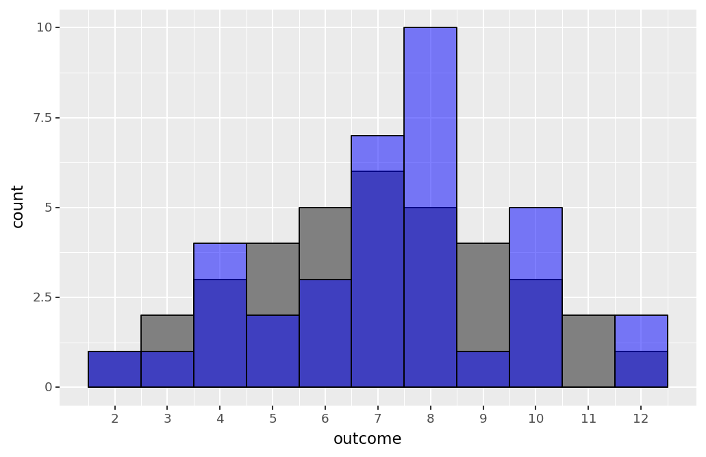
Imagine you have some data that is separated into categories. You are interested in determining if the frequencies (counts) in each category in your sample match those of the population. To answer this question, you can conduct a chi-square test! Here, "chi" is the Greek letter χ, which is pronounced "kai". For example, in the figure below, we show two histograms--the gray histogram is the theoretical rolls of two dice, while the blue is a sample of rolls. We could make some qualitative statements that compare the two plots. For instance, our sample includes more rolls of eight than the population, but the same amount of rolls of two. Often, however, we want to develop a more robust comparison than visual estimations. For this, we can conduct a chi-square test to confirm if the counts of each possible outcome are statistically significantly similar between the true population and the sample dataset.

Two Histograms of a Chi-Square Test

Credit: Eugene Morgan & Renee Obringer © Penn State is licensed under CC BY-NC-SA 4.0 [1]

To conduct a chi-square test, we first need to determine the hypotheses we will be testing. These hypotheses will look slightly different than those you learned in Lesson 5. As discussed in Lesson 5, the null hypothesis always uses equals signs. However, unlike the hypotheses in Lesson 5, for chi-square tests, the null hypothesis contains multiple proportions that are equal to the population proportions. Further, the alternative hypothesis is often written completely in words (i.e., no mathematical symbols). Generally, you can write something along the lines of "at least one proportion above is not as specified". An example of applying these hypotheses to the dice roll example is shown below.

Example of Hypotheses for Chi-Square Tests

$H_{0} : p_{2} = \frac{1}{36}, p_{3} = \frac{2}{36}, p_{4} = \frac{3}{36} \dots, p_{7} = \frac{6}{36}, \dots, p_{12} = \frac{1}{36}$

$H_{A} : At least one of the p's above is not as specified$

To conduct a chi-square test, you need to implement the following steps:

Define the hypotheses
Compute the expected count for each category: $n^{*} p_i$ where $n$ is the number of observations and $p_i$ is the population proportion
Compute the sample chi-square statistic: $x^{\land} 2 = s u m (frac {(observed count - {expected count)}^{\land} 2} {expected count}$
Find the p-value based on the idealized chi-square distribution, shown in the figure below
Make a conclusion based on the p-value

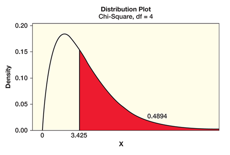
Generally, the chi-square distribution is find the p-value and make a subsequent conclusion. The chi-square distribution is interesting because it is always positive and is controlled by a single parameter, the "degrees of freedom", which we discussed in Lesson 6. Below, we show the distribution with 4 degrees of freedom. To calculate the p-value, we find the location of the test statistic and calculate the area under the curve and to the right of the sample statistic (this area is filled with red in the plot below). Generally, we will calculate the degrees of freedom as $k-1$ where $k$ is the number of categories in our dataset.

Distribution Plot Chi-Square, df=4

Credit: Eugene Morgan & Renee Obringer © Penn State is licensed under CC BY-NC-SA 4.0 [1]

Assess It: Check Your Knowledge

Knowledge Check

Chi-Square Test: Randomization Procedure

Read It: Randomization Procedure

Often, we will not have a large enough sample to conduct the chi-square test following the steps laid out in the previous discussion. In these cases, it is possible to conduct a randomization procedure to simulate additional data from a single sample and conduct a chi-square test. Below, we will demonstrate this process with a deck of cards. Our hypotheses are:

$Ho: p_{diamonds} = p_hearts = p_clubs = p_spades = 0.25$

$Ha: At least one of the proportions above is not as specified$

We will start with some data collection in the first video. Then, in the second video, we will demonstrate the randomization procedure. Finally, the third video will show the p-value calculation.

Watch It: Video - Data Collection (4:59 minutes)

Click here for a transcript.

Hello, and welcome to the lesson on chi-squared tests. So in this lesson the first part we're going to talk about chi-square tests, and in this video we're going to talk about how we can develop a randomization procedure for those chi-squared tests. Now the first step of any chi-square test, and for the majority of tests that we do in this course, is defining our hypotheses.

So here in Google Colab I have already defined our hypotheses. We have our null hypothesis that each suit in this deck of cards that I have is set to 25 percent each. In other words, this is a fair deck. There's the same percentage of hearts, as diamonds, as clubs, as spades. And then our alternative hypothesis is that one of those proportions is not as specified. It doesn't tell us which one, just that one of them is not. So, before we get started, I'm going to go ahead and draw some data from this deck of cards. So I'll go ahead and give it a shuffle. And essentially what I'm going to do is fill in this table here where I've got all zeros and I'm counting how many diamonds, hearts, clubs, and spades we get. So I'm just going to draw the top card from the deck until we've got about 20 cards drawn. And so, the first card I drew was a spade. So I come in here, increase that to one, got another spade, a heart, a club, another heart, heart, a club, spade, another spade. So right now we haven't got a lot of diamonds. Here's a heart, another heart, finally, a diamond.

So we've got about 10 so far. So here's another diamond, diamond, club, diamond, diamond, heart, heart. Oh, I did that wrong. This should be a seven, spade, diamond. And I will go ahead and stop there. We've got just over 20 data points there, so now we're going to continue with the coding portion of the lecture. And so, we now have our table, and this table is essentially, we're writing it in a dictionary, that's what these curly brackets mean. And then we're converting it to a data frame with the command PD data frame and then we're going to print the table. So I've already got my libraries added. So I'm just going to go ahead and print this table, which is essentially giving us the count. So we've got six diamonds, seven hearts, three clubs, five spades. And our goal with this will be to determine whether or not these observed proportions are essentially close enough to a 25 percent proportion. Or, whether that, whether they're not. And you know one sample isn't great in terms of our statistical analysis, and so what we're going to do is create that randomization procedure that we've done, a similar one to what we've done before, so that we can generate more samples.

Credit: © Penn State is licensed under CC BY-NC-SA 4.0 [1]

Watch It: Video - Randomization (8:40 minutes)

Click here for a transcript.

And so, I've laid out a few steps here. So our first step is to calculate the sample statistic. And in particular, our chi-squared statistic is the sum of this fraction. We've got our observed counts minus our expected counts squared, divided by the expected counts, and then all summed together.

And so, in order to calculate this chi-square sample, first we need to get our observed counts, and our expected counts. Our observed counts are what we see here, so we need to calculate the expected counts and then we need to do this summation. A,nd so the first thing that we'll do is determine the sample size. So I'm going to take this table variable up here, I'm going to do the count column, so table dot count. And this is referring to the column count. And then I'm going to sum that. So essentially, by summing all of our counts we can actually get our sample size. And then I can print that, so we can see what it looks like - twenty-one cards drawn.

Next we need to get the expected counts. And so, I'm going to create a new array using this numpy dot array command, which is essentially just all of my expected proportions. Now this is what we wrote up here in our null hypothesis, 0.25, and it's the same for each category. And so, that is my expected probability, my proportion. And so then, my count exp is just my sample size, times my proportions. And we can print that at the end.

And so we can see that it's all the same because they all have the same proportion. But the chi-square test compares counts to each other. So we need to somehow take that proportion into account, and that's what we're doing here. So in theory, we would have 5.25 cards of each suit. Now that isn't actually possible, but that is sort of the ideal count based off of our sample size, 21. And so, then the next step is to actually calculate the chi-square statistic. So I'm going to call this chi-square underscore samp, because it's my sample statistic. I'm going to do two sets of parentheses and in the first parentheses I'm going to take my observed count, so this is following this function up here. So my observed count minus my expected count, squared. So in Python when we want to do an exponential, we do two asterisk.s And then I divide that by my count EXP. And then outside of all the parentheses, I sum it. So we can run that. And now I have my sample chi-square value as 1.66.

And so, this is the first step to developing our randomization procedure. The next step is actually implementing that randomization. So once again we're going to be using this NP random choice, which we're quite familiar with at this time. And in particular, we're going to replace equals true. And so, the first step within step two, is to initialize the variables. So we need to tell it how many iterations we want to do. And I'm going to set up an empty array.

And then we can start the procedure. So we can say for i in range of n, similar to what we've done before, and then I'm going to create a new variable that I call sim suits. And this is what's going to randomly draw a suit from our options. So we can say np dot random choice, and I'm just going to draw from table suit. And if we scroll back up here, we can see that the suit column in our table data frame is diamonds, hearts, clubs, or spades. So it's just going to draw one of those categories, similar to drawing a card. Then, slightly different from what we've done before, we need to define the probability at which to draw those suits, twenty five percent each. We define how many we want to draw, our sample size, lowercase n. And we replace equals true, so that we don't run out of suits. So this will be our simulated draws, but we need to make sure those get into counts, which is what the chi-squared test compares. And so, we can say sim underscore counts. And so, in square brackets I'm going to say sum or sim suits equals equals diamonds. And then comma, our next point in the array is the sum of where sim suits equals equals hearts. And I missed a parenthesis right there. So each of these summations needs its own parentheses so that we can read it. I'm going to enter down in between because it's still wrapped in the square brackets, Python knows it's still part of the same command. So then I do sim suits equals equals clubs. And then finally the sum of sim suits it equals spades. And so this will be my simulated count variable.

And then last but not least, we need to use that simulated count variable to calculate our sample, sampling distribution, our randomization chi-squared. So this is where our empty chi-square array comes in. Set the ith term equal to sim suits, or sim counts, minus count exp, which is what we defined up here, squared, divided by count exp, and then summed together.

So, we can run this, and then we can see what the chi-square looks like, just an array, a very long array. So I won't keep that there but good to know that it worked. And so, then the next step is actually calculating our p-value.

Credit: © Penn State is licensed under CC BY-NC-SA 4.0 [1]

Watch It: Video - P-Value (2:39 minutes)

Click here for a transcript.

Credit: © Penn State is licensed under CC BY-NC-SA 4.0 [1]

Try It: DataCamp - Apply Your Coding Skills

Use the card drawing simulator linked here [2]to draw cards for your own sample. Then, apply the randomization procedure for the chi-square test.

1
2
# libraries
import numpy as np
XXXXXXXXXXXXXXXXXXXXXXXXXXXXXXXXXXXXXXXXXXXXXXXXXX

XXXXXXXXXXXXXXXXXXXXXXXXXXXXXXXXXXXXXXXXXXXXXXXXXX

1/0 0/0

Powered by DataCamp

Assess It: Check Your Knowledge

Knowledge Check

Chi-Square Test: Visualization

Read It: Visualizing Chi-Square Distributions

When creating visualizations for chi-square tests, you need to provide three key pieces of information: (1) the randomization distirbution of chi-square statistics, (2) the sample chi-square statistic, and (3) the idealized chi-square distribution. In the video below, we walk you through adding each of these parts to a single ggplot graph.

Watch It: Video - Visualization (7:06 minutes)

Click here for a transcript.

Welcome back to our video series on chi-squared tests. In this video we're going to talk about how we can visualize our chi-square randomization distribution, as well as an idealized chi-square distribution. And so, we're essentially going to make a histogram, but we're going to use a different way, different variable on the y-axis than we have in the past. So let's go ahead and get started. So, with our ggplot, our data is chi-square df. And this is part of the reason why up here we convert it into a data frame. And then we can say geom histogram, and then we have our aes statement. Our x is just chi-square, which is what we called our data. And then normally, we would leave this as it is and do a bit of a count. But we can say y equals after stats density in quotes. So this essentially tells Python to apply the density command to the data, rather than the count that is traditionally shown in a histogram. And then we can also define an outline color as black, and we can specify our bin width as 0.75. And then as we've done in the past, we can add a vertical line for our sample statistic, which is chi-square samp color is blue. And we can say line type dashed. And so here we have our our chi-square sampling distribution of the histogram and what the sample is. And so as the way the p-value works, all of the data that is above our sample statistic goes into our p-value. Which is why we have such a high one. You can see that a lot of that data is above the sample statistic.

But often it can be very helpful to show the idealized chi-square distribution. And so a chi-squared distribution, similar to the normal distribution that we learned in a previous lecture, is an idealized distribution that depends on only the degrees of freedom. And it'll generally follow this right-skew shape. So before we can actually get into the plotting, we do need to do a bit of prep work. First we need to define our degrees of freedom. And we're going to define this as 3. And officially, this is the number of categories, minus one. So we've got four suits, four categories, three minus one, or four minus one is three. And then we also need to create new columns in our chi-square df. So we need one for x pdf, and this is just a series of numbers that match the x-axis we see here. So we do np dot bin space 0 to 25, to 1000, or, with 1000 in-between. Effectively, this creates a series of numbers from 0 to 25, evenly spaced numbers from 0 to 25, and there's 1,000 values. And so, in effect this will count from 0 to 25, with putting a thousand values in between. And then we need the y pdf's. And this is where we actually figure out what the chi-squared distribution is that fits this data. And so we say stats dot chi-squared dot pdf. We give it our idealized x data, and we give it the degrees of freedom.

And so, now if we look at just the first five rows, we can see we've got our original chi-square sampling distribution, then we've got idealized x and y data. And so, if we want to plot this we can just continue on with our plot that we did last up here. And essentially, we can just add another line plot on top of it, where our x value is now x pdf, our y value is now y pdf. The color is blue, and I'm going to give it a size to make it a little bit more obvious. And so, here we can see the final plot where we've got our chi-squared distribution. We've got our idealized curve, here. And we can see that it does a pretty good job of following the data. And that is in effect, a way that we can see what the idealized chi-square curve is going to look like.

Credit: © Penn State is licensed under CC BY-NC-SA 4.0 [1]

Try It: GOOGLE COLAB

Click the Google Colab file used in the video here [3].
Go to the Colab file and click "File" then "Save a copy in Drive", this will create a new Colab file that you can edit in your own Google Drive account.
Once you have it saved in your Drive, try to edit the follwoing code to create a visualization of the data you collected in the previous DataCamp exercise.

Note: You must be logged into your PSU Google Workspace in order to access the file.

1

2

3

4

5

6

7

8

9

10

11

12

13

14

15

16

17

# Copy your data from the previosu DataCamp exercise
table = pd.DataFrame({'Suit' : ['Diamonds', 'Hearts', 'Clubs', 'Spades'],
                                'Count' : [0,0,0,0]})
 
# Rerun randomization procedure code
 
# Create Visualization
deg_f = ... 
 
chisq_df['x_pdf'] = ...
chisq_df['y_pdf'] = ...
 
(ggplot(chisq_df) +
    geom_histogram(...) +
    geom_vline(...) +
    geom_line(...)
)

Once you have implemented this code on your own, come back to this page to test your knowledge.

Assess It: Check Your Knowledge

Knowledge Check

Chi-Square Test: One Line Test

Read It: Chi-Square One Line Test

Similar to the one-line hypothesis tests discussed in Lesson 6, there is also a one-line test for chi-square tests. This test uses the stats.chisquare command in the scipy.stats library, the documentation for the command can be found here [4]. In order for this test to work, you need to provide f_obs (the observed count) and f_exp (the expected count). Below we demonstrate how to implement this code.

Watch It: Video - Chi-Square One-Line Test (2:46 minutes)

Click here for a transcript.

Credit: © Penn State is licensed under CC BY-NC-SA 4.0 [1]

Try It: GOOGLE COLAB

Click the Google Colab file used in the video here [5].
Go to the Colab file and click "File" then "Save a copy in Drive", this will create a new Colab file that you can edit in your own Google Drive account.
Once you have it saved in your Drive, try to edit the following code to implement the one-line test using the card data you collected earlier in the lesson:

Note: You must be logged into your PSU Google Workspace in order to access the file.

1

2

3

4

5

6

7

8

9

10

11

12

# Copy your data from the previosu DataCamp exercise
table = pd.DataFrame({'Suit' : ['Diamonds', 'Hearts', 'Clubs', 'Spades'],
                      'Count' : [0,0,0,0]})
 
# find expected counts
n = ...
p = ...
count_exp = ...
 
# implement one-line code
results = stats.chisquare(f_obs = ..., f_exp = ...)
print('p-value: ', ...)

Once you have implemented this code on your own, come back to this page to test your knowledge.

Assess It: Check Your Knowledge

Knowledge Check

Another Example of Chi-Square Tests

Read It: Another Example of a Chi-Square Test

So far in this lesson, we have been working with an example where all the expected proportions were equal. However, often the proportions we were work with are not expected to be equal. This situation increases the complexity of our chi-square test, since we need to make sure we are ordering things correctly within our expected counts array. Below, we demonstrate how to implement a chi-square test with unequal groups.

Watch It: Video - Chi-Square Test Part 2 (9:02 minutes)

Click here for a transcript.

Welcome back to the videos in chi-squared testing. In this lesson, in this video, we're going to go over another way that you might encounter chi-square testing. So, in the previous set of videos, we had a deck of cards that was all that had equal proportions across each of the suits. But oftentimes our populations won't have equal proportions across all groups. And so, in this video I'm going to show you how you can do a chi-square test where we have different populations across groups.

So here in this code, I'm calling it chi-square test part two, we've got some data on undergraduate enrollment in the College of Earth and Mineral Sciences in the Fall of 2022. And our goal is to compare the enrollment in the whole College of Earth and Mineral Sciences to enrollment in one of the courses we taught during the academic year. And so, our null hypothesis is that, is just each proportion based off the total enrollment on EMS. So, we can see that each major, EBF, Energy Engineering, Environmental Systems, and so on, has a different proportion of students. And then our alternative hypothesis is that at least one of these is not as specified. And so, we can go ahead and run the code that I've already got set up, which is essentially to read in the first week survey data. We can see that we've extracted just the majors from that survey. And then we can start by figuring out the count. So, before we were doing... so, we already knew the count right off the bat. But in this case, we need to actually extract amounts. So, we use this dot value counts command to do that. And we can see that we've got some other data. And we've got this Energy Engineering other data that we, that isn't going to work with our existing data set because we don't have any proportion specified for the other, or for dual majors. And so, we can go ahead and update this. First, we're going to account for this one dual major, here. We still want them to count towards the Energy Engineering count, but we don't need the other dual majors, so we can say dot replace. And so essentially, we're just going to replace comma other with nothing, empty quote open close quotation nothing, there. So, we can do that. And then we also need to remove these other majors. We don't know what major they are, so we can't count them towards any of the existing majors. So, we can just say that we want only the majors that are not equal to other.

So that ran, and then we can recount the data, this time storing it in accounts variable. So we can say majors needs to be plural there, dot value counts. Go ahead and print the counts. So here we can see how our counts actually work now that we've removed the other and added that dual major into Energy Engineering. So, this is our observed counts. The next step in our chi-square procedure is develop the existing or the expected counts, so counts_exp, is just counts dot sum. So this is our sample size of our observed data, times the array of proportions. And now, before, our array of proportions was just four times 0.25, but now that our proportions appear, are different for each category, we now need to manually import each of those. And a very critical point here; the order has to be the same as the order up here, because we ultimately are going to be comparing these two values. And so, we need to make sure that the order is the same across both observations and expected count. And so, I've listed the order here that is based off of this order. So we can do 0.493, for pp and g points 172, 0.163, and 0.04. And these values also match what we have up here in our null hypothesis.

So we can run that. We get our expected counts and then we can run the chi-square test. And for this purpose, I'm just going to do the one-liner. So we already know how to do the randomization procedure, but in this case, we'll just do the one- liner. So we say stats dot chi square. Our observation, we call it counts. Our expected values we call counts_exp. And then we can print p-value, which is just results dot p-value.

And so, then we can see the p-value is .017. And so we can write our conclusion. The p-value is less than 0.05, our significance level, so we reject the null hypothesis in favor of the alternative, that at least one of the proportions is not as specified. At least one, however, this chi-squared test doesn't tell us which one is different. It just tells us that at least one, at least one is different. And so, in order to actually get an idea about which one is different, we can just subtract our expected counts and our observed counts. And so, here we can see that the most extreme difference is png e, which had 11 more actual attendance than expected. Since the value is negative, that means observation is greater than expected. Meanwhile, the Environmental Systems group had nearly six less than expected. And so, we can then start to make some, have a discussion about which of these majors are primarily responsible for the rejection of our null hypothesis.

Credit: © Penn State is licensed under CC BY-NC-SA 4.0 [1]

Try It: GOOGLE COLAB

Click the Google Colab file used in the video here [6].
Go to the Colab file and click "File" then "Save a copy in Drive", this will create a new Colab file that you can edit in your own Google Drive account.
Once you have it saved in your Drive, try to edit the following code to conduct a one-line chi-square test with unequal groups. Remember to match the order of your expected counts to that of your observed counts!

Note: You must be logged into your PSU Google Workspace in order to access the file.

1

2

3

4

5

6

7

8

9

# Determine the count of each major
counts = ...
 
# calculate expected counts 
counts_exp = ...
 
# run the chi-square test
results = ...
print('p-value: ', ...)

Once you have implemented this code on your own, come back to this page to test your knowledge.

Assess It: Check Your Knowledge

Knowledge Check

Two-Way Chi-Square Tests

Read It: Two Chi-Square Test

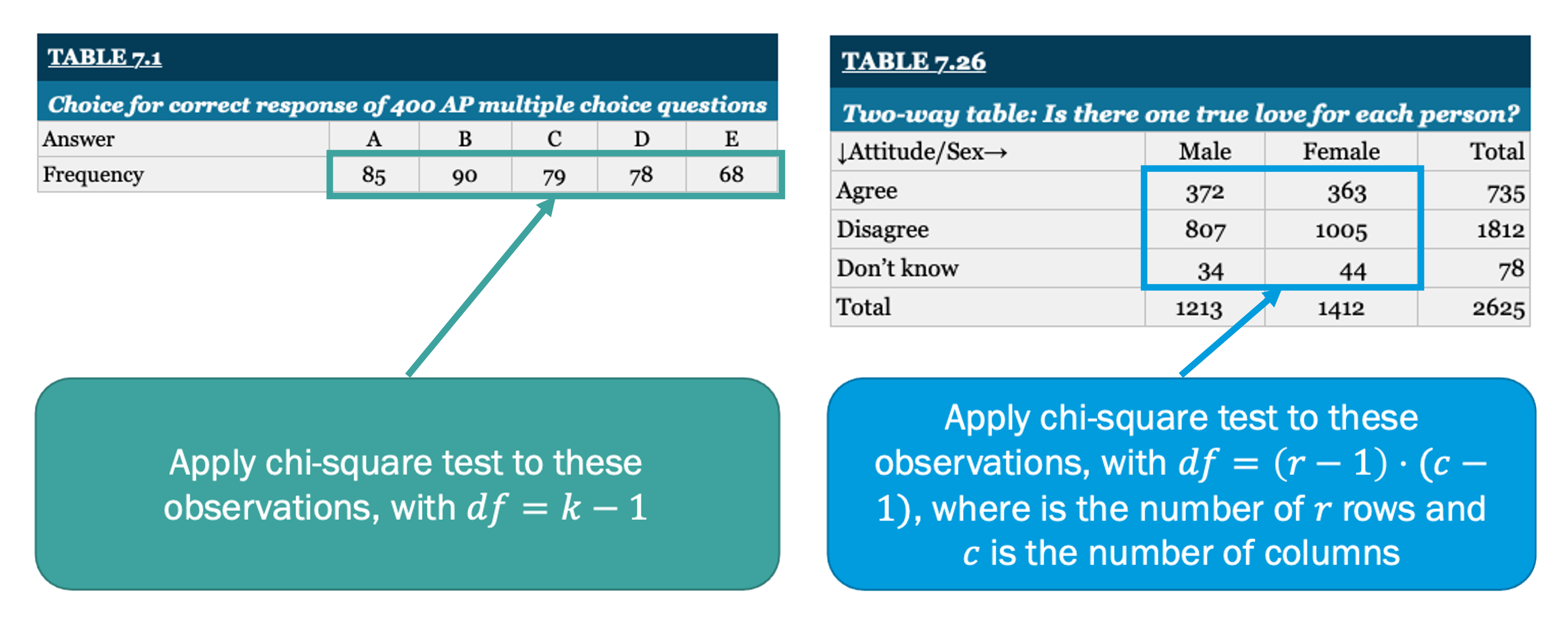
So far in this lesson we have focused on one-way chi-square tests. These tests focus on comparing one categorical variable to known proportions. There is, however, another version of the chi-square test known as the two-way test. Two-way chi-square tests compare two categorical variables, rather than one. Additionally, the degrees of freedom are calculated differently: $df = (r - 1) times (c - 1)$ where $r$ is the number of rows and $c$ is the number of columns. Below, we demonstrate two tables that might be used in chi-square tests. The table on the left shows a single categorical variable, for which we would conduct a one-way chi-square test. Conversely, the table on the right shows a two-way table (e.g., there are categorical variables along the rows and columns), for which we would need to conduct a two-way chi-square test.

Two-way chi square table vs One-way. See image description below

One-Way vs. Two-Way Tables

Credit: © Penn State is licensed under CC BY-NC-SA 4.0 [1]

One-Way Table: One categorical variable
Table 7.1
Choice for correct response of 400 AP multiple choice questions
Answer	A	B	C	D	E
Frequency	85	90	79	78	68

Two-Way Table: Two categorical variables
Table 7.26
Two-way table: Is there one true love for each person?
Attitude/Sex	Male	Female	Total
Agree	372	363	735
Disagree	807	1005	1812
Don't know	34	44	78
Total	1213	1412	2625

Below, we provide a demonstration of a two-way chi-square test using the card drawing activity from earlier. In particular, we will use the stats.chi2_contingency command from the scipy.stats library. You can read more about this command here [7].

Watch It: Video - Two-Way Test (9:00 minutes)

Click here for a transcript.

Welcome back to the final video on chi-squared testing. So, in this video, I'm going to show you how we can conduct a two-way chi-square test. And so, our two-way chi-square test ends up looking a little different in terms of the null hypothesis. Essentially, we're looking at association in instead of equal proportions.

So, what we're going to do is we're going to do another card based draw, and we're essentially going to compare the suit to the chance of winning the game. And so, our null hypothesis is that there's no association between the suit that you draw and the chance of winning the game of war, meaning the highest card wins. An alternative is that there is an association. So, I've already done some setup here to get our data in a way that we can use this two-way table. And so, I'm using a new command called product, and then I'm using that to essentially build up this list of parentheses and then creating this data frame.

And essentially, what we're going to do when I draw cards, is that we're going to draw two cards at once, and we're going to count which one wins and record the suit. So, we're going to add a third column to this table and do some counting there. So, here I've got it set up. Table two count is going to be what we call it. And so, I've got six of hearts and four of hearts here. So, that means that hearts actually gets one loss and one win, and we're going to ignore any ties that we get. So, then the next two cards I have the nine of hearts and the queen of clubs. So, that means hearts get a loss and clubs gets a win.

Then I have a tie between two nines, so I'm just going to ignore those. Then I have the nine of diamonds and the six of clubs. So, that means clubs gets its first loss and diamonds gets its first win. Then I have king of clubs and five of spades. So, clubs gets a second win and spades gets a loss.

So, that means spades gets a win and a loss. Four of diamonds and three of spades. So, spades gets another loss and diamonds gets a win. Another tie. Queen of spades and ten of spades. So again, win and a loss, a tie, two tens. We've got an ace of clubs and an eight of hearts. So, that means clubs gets a win and hearts gets a loss. An ace of hearts and a three of clubs. So, hearts gets a win and clubs gets a loss.

So, spades gets a win, diamonds gets a loss, and we will do one more draw. So, a ten of diamonds and a three of hearts. So, diamonds gets a win and hearts gets a loss. And so, what we're going to do in the rest of this video is conduct a two-way chi-square test to see if there's any association between the suit and the chance of winning. And so, here we have our table just to show you what it looks like. We can run this. So, now we have the suit, whether or not they won and the count of that situation happening. And so, the first thing we need to do to conduct the two-way chi-square test is we need to reorganize this using cross tab. So, I'm going to call this table three, and I'm going to say PD cross tab.

We want to do table two of suit and table two of win with question mark. And then we want the values to be table two count. And then I'm going to specify that the app function is np dot sum and that the margins are set to false.

So, we can print this. And we can see that we've got essentially the wins no and yes, and we've got the suit. And that's the format that we need our data to be in. Because then when we conduct the test, we can say results equals stats dot chi-square, this time, underscore contingency. And then we just give it what we called our two-way table, table three. And we can print those results to show you what it looks like. So, they give us the chi square statistic, they give us the p value, the degrees of freedom, and they give us what the expected frequency is. So, a little bit more information than we see from the one-way chi-square test. But if we just wanted to print the p value, we can just say results one, which is this is the 0th point, so this is the first point. So, we can print that, and we can see that it's the same value .57. And so, we can draw a conclusion from that. We can say that the p value is greater than our 0.05.

So, there is not sufficient evidence to say there is an association between suit and winning. In other words, our null hypothesis that we are accepting says there is no association. And so, that is the conclusion that we make from this two-way chi-square test.

Credit: © Penn State is licensed under CC BY-NC-SA 4.0 [1]

Try It: GOOGLE COLAB

Click the Google Colab file used in the video here [8].
Go to the Colab file and click "File" then "Save a copy in Drive", this will create a new Colab file that you can edit in your own Google Drive account.
Once you have it saved in your Drive, use the card drawing simulator linked here [9] to create some data and implement a two-way chi-square test:

Note: You must be logged into your PSU Google Workspace in order to access the file.

1

2

3

4

5

6

7

8

9

10

11

12

13

14

15

16

17

# draw cards and populated the table with the number of wins and losses by suit
table2['Count'] = [0, 0, # diamonds
                   0, 0, # hearts
                   0, 0, # clubs
                   0, 0] # spades
 
# reorganize the table using pd.crosstab
table3 = pd.crosstab(table2['Suit'], table2['Win?'], 
                     values = table2['Count'], 
                     aggfunc = np.sum, margins = False)
 
# conduct test
results = ...
results
 
# print p-value
print('p-value: ', ...)

Once you have implemented this code on your own, come back to this page to test your knowledge.

OPTION 2 : DATACAMP

Try It: OPTION 2 DataCamp - Apply Your Coding Skills

Dictionaries are a quick way to create a variable from scratch. However, their functionality is limited, so we will often want to convert those dictionaries into DataFrames. Try to code this conversion in the cell below. Hint: Make sure to import the Pandas library.

1
2
# Create a Simple Dictionary
mydict = {'Name':['Amy', 'Bob', 'Clair', 'Daisy'],
XXXXXXXXXXXXXXXXXXXXXXXXXXXXXXXXXXXXXXXXXXXXXXXXXX

XXXXXXXXXXXXXXXXXXXXXXXXXXXXXXXXXXXXXXXXXXXXXXXXXX

1/0 0/0

Powered by DataCamp

Assess It: Check Your Knowledge

Knowledge Check

ANOVA

One-way ANOVA

ANOVA (short for "Analysis of Variance"; more on that later) allows one to compare means across multiple groups. Here, we will just focus on one-way ANOVA, where we compare means across more than two categories of a single categorical variable. Recall that in Lesson 5 we did a comparison of means (difference of means hypothesis testing). Well, ANOVA essentially expands that comparison to more than two groups or categories so that you can efficiently see if there is a significant difference of means across many groups in just one test. Thus, it is similar to a chi-square test, except ANOVA looks at means whereas chi-square testing looks at proportions.

One-Way Chi-square vs. One-Way ANOVA
Hypothesis for a One-Way Chi-square Test are:	Hypothesis for a One-Way ANOVA Test are:
H_o: Defines proportions, $p_{i}$ , for all $k$ categories	H_o: All population means, $μ_{i}$ are equal for all $k$ categories
H_a: At least one $p_{i}$ is not as specified	H_a: At least one $μ_{i}$ is not equal to the others

Another way of stating the null and alternative hypotheses for one-way ANOVA is:

\begin{align} H_O:&\ \mu_1 = \mu_2 = ... = \mu_k \\ H_A:&\ \text{at least one mean is not equal to the others}\end{align}

Since chi-square tests look at proportions, they are suited for a categorical variable, which would then be summarized by a frequency table.

Data for a One-Way Chi-square test. See link in caption for text description

A generalized depiction of the typical data format for chi-square tests

Click for a text description of Data for a One-Way Chi-square Test.

Data for a One-Way Chi-square test
Categorical Variable
A
B
B
A
C

Data for a One-Way Chi-Square Test
Categorical Variable	Frequency
A	2
B	2
C	1

Credit: © Penn State is licensed under CC BY-NC-SA 4.0 [1]

On the other hand, ANOVA examines means and so is meant for a quantitative variable, which can be summarized into grouped sample means.

Data for a One-Way ANOVA test. See link in caption for text description

A generalized depiction of typical data for a one-way ANOVA test

Click for a text description of Data for a One-Way ANOVA Test.

Data for a One-Way ANOVA test
Categorical Variable	Quantitative Variable
A	5
B	4
B	3
A	3
C	6

Data for a One-Way ANOVA Test
Categorical Variable	Mean
A	4
B	3.5
C	6

Credit: © Penn State is licensed under CC BY-NC-SA 4.0 [1]

Analysis of Variance

The key question that ANOVA answers is: “Are the differences in the mean values significantly different?” Most likely, the sample means from each group do not agree exactly. So, how much disagreement in the sample means is needed to say that there is difference in the population means?

This is exemplified in the figure below, where one may be able to tell that the sample means (represented by asterisks) are different, but it’s hard to tell whether these differences matter much because the samples themselves (the boxplots) overlap so much.

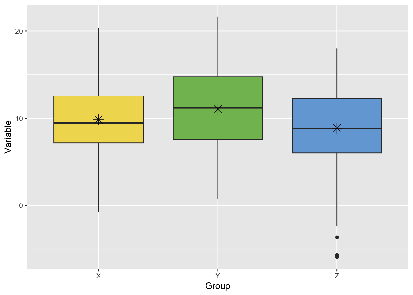
Comparative boxplots of three different samples, X, Y, and Z, of a quantitative variable ("Variable"). The asterisks denote the sample mean of each group.

Credit: © Penn State is licensed under CC BY-NC-SA 4.0 [1]

To answer this, we need to consider how much the sample means could vary by random chance alone (that is, from randomly drawing the sample from the population). Therefore, we need to analyze the variance in the sampling distribution of the mean. Continuing with the example above, the figure below shows the corresponding bootstrap distributions for each sample mean (recall from Lesson 4 that the bootstrap distribution approximates the sampling distribution). We can now see that the sample means are distinct from one another. The variances of the sample means (the spread of each boxplot) aren’t so large as to overlap with each other.

Comparative boxplots of the bootstrap distributions of sample means from the samples in the figure above

Credit: © Penn State is licensed under CC BY-NC-SA 4.0 [1]

FAQ

The F-statistic

ANOVA breaks up the total variability of the sample values into two kinds of variability: 1.) the variability within the groups and 2.) the variability between the groups. If the variability between the groups is large compared to the variability within the groups, we can say that the groups have different means. In equation form, this idea is noted:

$SS_{Total} = SSG + SSE$

The terms are defined as:

$SS_{Total}$ : the total sum of squared deviations. This takes the distance of each data point from the mean of all data, squares that distance (so they’re all positive), and adds them all up. Thus, it measures the TOTAL VARIABILITY of the data.
$SSG$ : the sum of squared deviations for groups. This takes the distance of each group’s mean from the mean of all data (ungrouped), squares that distance, and adds the values up. Thus, it measures the VARIABILITY BETWEEN GROUPS.
$SSE$ : the sum of squares for error. For each group, this takes the distance of each data point in the group from the mean of that group, squares that distance, and adds them all up. Thus, it measures the VARIABILITY WITHIN THE GROUPS.

Our goal with the ANOVA test is to compare the variability BETWEEN groups to the variability WITHIN groups, however we can’t properly compare $SSG$ to $SSE$ directly since these use different amounts of data. So we need to look at the “mean square” for each:

$\begin{align} \text{Mean square for groups: } MSG &= \frac{SSG}{k-1} \\ \text{Mean square for error: } MSE &= \frac{SSE}{n-k} \end{align}$

Here, $n$ is the total sample size (number of data values in all groups together) and $k$ is the number of groups. The denominators, $k-1$ and $n-k$ represent the “degrees of freedom” (“df” or “dof” for short) for each term. We can then find the F-statistic as:

$F = \frac{MSG}{MSE}$

which effectively compares the variability BETWEEN groups (numerator) to the variability WITHIN groups (denominator). Thus, if the null hypothesis is true and the group means are actually equal, we expect the F-statistic to be about 1. Larger values of the F-statistics indicate a larger $MSG$ relative to $MSE$ , and thus a difference in means (or at least one mean).

The F-distribution and p-value

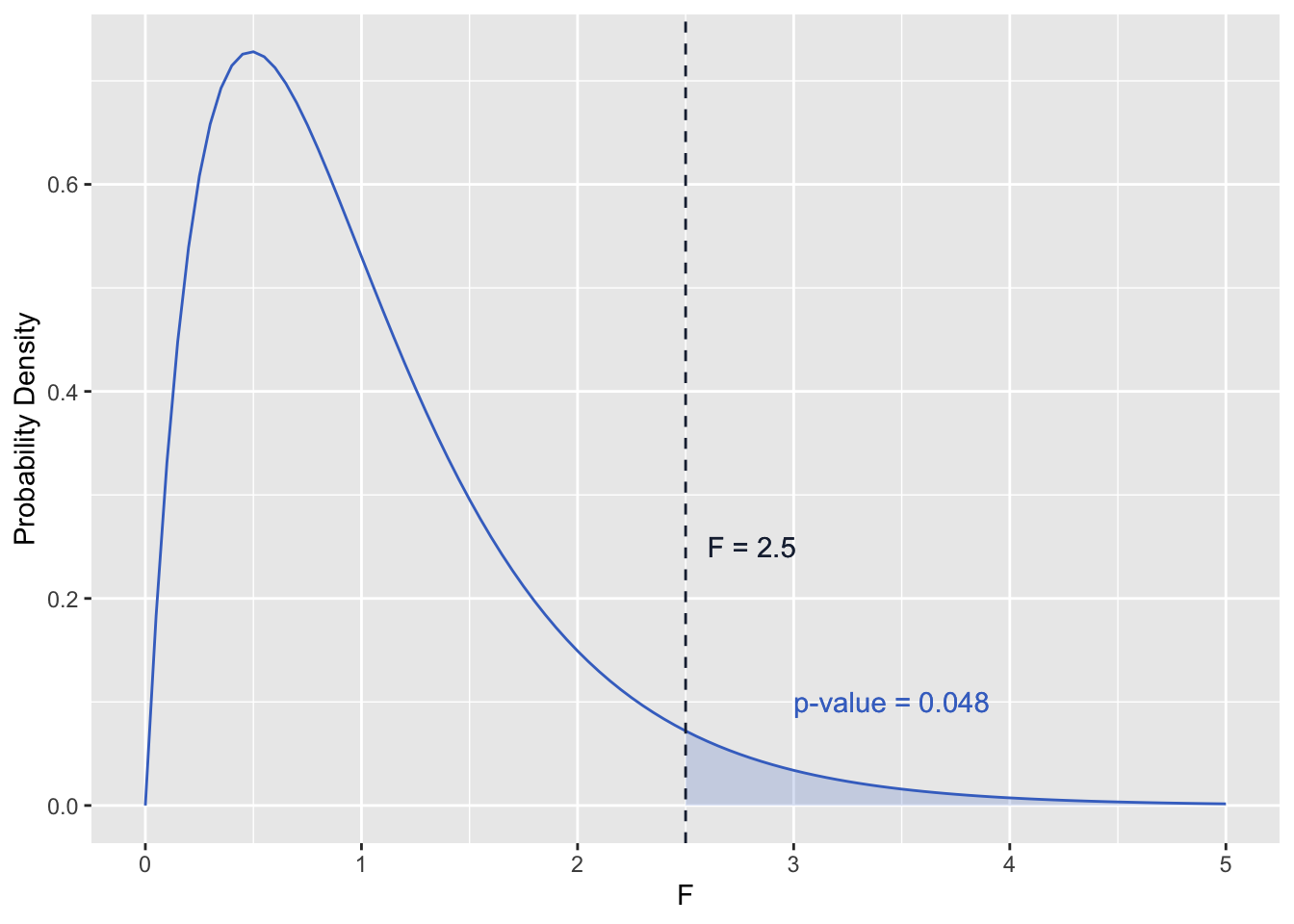
The p-value for our ANOVA test depends on the F-statistic above and the degrees of freedom. The degrees of freedom determines the shape of the probability density function for F (an example is pictured below). The p-value is then the area under the probability density function and GREATER THAN the F-statistic calculated from the sample data (shaded area in the figure below).

In this figure, the curve is the probability density function for F with degrees of freedom k − 1 = 4 and n − k = 95. The p-value is the shaded area under the curve and greater than the F-statistic value of 2.5, in this example.

With the degrees of freedom staying constant, a larger F-statistic corresponds to a lower p-value.

One-way ANOVA Table

To facilitate an understanding of where the variability in the data is coming from, sometimes the results from an ANOVA test are presented in a table, typically taking the following format:

The typical format of a one-way ANOVA table.
Source of Variation	Degrees of Freedom	Sum of Squares	Mean Squares	F	p-value
BETWEEN	$k-1$	$SSG$	$MSG$	$\frac{MSG}{MSE}$	Area under F-distribution and greater than F-statistic
WITHIN	$n-k$	$SSE$	$MSE$
TOTAL	$n-1$	$SST$

FAQ

One-way ANOVA: One Line Test

Read It: One Line Test

In this lesson, we won’t go into how to perform ANOVA using randomization distributions, but instead we’ll rely on the one-way ANOVA test function that available in scipy.stats, which is called f_oneway. The basic usage of this function requires one to input an argument for each group or category, and that argument is the series of values belonging to each group. Following the example above, we’d have:

import scipy.stats as stats
A = [5, 3]
B = [4, 3]
C = [6]
stats.f_oneway(A, B, C)

Note that we don’t have to calculate the mean for each group; f_oneway does that for us and we just need to supply the data values. More samples can be added in the analysis, just by including them as additional arguments separated by commas. Also, be sure to remove any NA/NaN values first!

The output from f_oneway is the F-statistic and the associated p-value.

Video: L07V08 ANOVA (29:42)

Credit: Dutton Institute. "L07V08 ANOVA [10]." YouTube. November 1, 2023.

Click here for a transcript of the L07V08 ANOVA video.

Hi. In this video, we're going to walk through an example of one-way ANOVA. And in this analysis, the example we'll use comes from research conducted by people in my own department. That's the Department of Energy and Mineral Engineering here at Penn State. So, the researchers here predict the volume of emissions that will come out of PA based facilities under three different policy scenarios.

Scenario one is the base case, which is that PA does not join the Regional Greenhouse Gas Initiative, which is essentially a cap and trade program, and keeps the existing alternative energy portfolio standard, which mandates a certain amount of energy has to come from alternative energy sources. Our second scenario is that PA joins RGGI and keeps the portfolio standard. And then the third scenario is that the PA joins RGGI but drops the portfolio standard. It should be noted that this research was conducted in 2021 before Pennsylvania joined RGGI in the summer of 2022. So, let's get down to the analysis. .

So, our hypotheses, which we'll always have with ANOVA, are that all three means across all three groups are equal. So, our three groups are the three different policy scenarios, and our quantitative variable here is the volume of emissions. To simplify things, we're just going to look at the volume of nitrous oxide. But do bear in mind that the data set does contain other pollutants as well, if you want to look at those. So, we're saying that the volume of nitrous oxide on average is equal across the base case scenario RGGI and no AEPS. .

The alternative is that at least one of these means is not equal from the others. So, let's get down to it. Let's see what the data say. So, first things first is to import the data, and I've already done that with these familiar commands here. One thing that should be noted is that we've got three distinct Excel sheets. .

So, we're going to read directly from Excel using read underscore Excel, this function from Pandas. We can do that, which is nice. Another thing, too, is to simplify this analysis, we're only going to look at the year 2030. So, if you open up one of these Excel files, you'll note that it's got multiple spreadsheets by year. And so we're just going to pull out the sheet for year 2030. .

So, we've imported these three Excel sheets as data frames called Base RGGI and no AEPS. Let's examine one. Let's just take a look at base here. .

And so, here's our data. Now, the task at hand for data processing is that we need to merge all three of these data frames. So, if we want to compare these three, it's helpful to have them in one data frame so that we can make a fair comparison using our statistical tools here. So, first things first is if we're going to merge these, we need to go back and use our merge function that we learned about in lesson two. And we need to identify some keys for doing this merging. .

And so, we can tell the merge function what our key variables are by setting them as indices. So, we'll use the set index command to define the key variables. And these are the variables that uniquely identify the rows here. So, we need to provide a list here and the variables that do that, If you go and inspect the data set, is the unit unique ID, the latitude, the longitude, the state, the county and the fuel type. Okay. .

And we'll use these same ones. So, all three of those data frames are structured the same and have the same variables. So, we'll do this for all three data frames that we have here and just change these names. So, RGGI and no AEPS. .

Okay, so all the set index function is doing is designating these variables as indices. Another thing that we'll do to set up the data before doing the merging is to add a suffix to the variables in the data frames. And what this will allow us to do is distinguish the variables that are in base from the variables in RGGI and from the variables in no AEPS because these variables are all currently called the same thing because they're in separate data frames. But when we merge them together, we don't want to get confused about which column belongs to which. So we'll add a suffix to just make sure that they're distinct. .

So, use this add suffix command and to base we'll add the suffix underscore base and same thing with RGGI and no AEPS, except we want to change these suffices to RGGI and no AEPS. Okay? And then we can do the merging. So, we'll make a new data frame, let's call it DF underscore merged stand for data frame that is merged. And from the Pandas library we'll use our merge function and we can't merge all three at once. So, we'll merge two into one data frame and then this merge data frame will merge with the third item. So, let's first start off by just merging Base and RGGI. .

Our left index here we'll say left index is true and right index is true just to indicate that we're using the indices here and we want to keep everything. So, we'll say how is equal to outer. So, we're going to do an outer merge in order to keep everything. And then once these two are merged, what we'll do is we'll overwrite our DF merged again using the merge command here and we'll use all of these same settings except instead of Base, we're going to use DF merged. So we're going to first merge Base and RGGI store that in DF merged and then DF merged is going to be used in another merge command to attach not RGGI but the no AEPS data frame. .

Okay? And then we'll visualize how that plays out. Okay, so we'll go ahead and run this and there we go. So, note that these items that are in bold, these are the indices. So from setting the index, these are all in bold here. .

And then we've got and then we've got all our variables. So, the different pollutants here's NOx that we'll be looking at. And note that we've attached the underscore base to distinguish that from the NOx that's currently hidden by this dot, dot, dot, but the NOx for underscore RGGI and no APS. Okay, so that all worked well. And you might be wondering, oh, why did we include latitude, longitude, state, county and fuel type in the indices, even though that they're not really keys. That we've got the same values across these first five entries, for example, for those variables. .

Whereas really unit unique ID is really the key here in that it's the unique identifier for each row. Well, it doesn't hurt to include these variables in the keys and essentially retain them for the items. These are properties of the individual units. The units here are basically power plants, factories and things like that. And so, we can retain these variables by including them in the indices without duplicating them across all the different data frames that are merged in here.

So anyway, a little bit about that. So, let's move on. So, once we've done that, let's take those variables that we have set as indices and bring them back as variables. So, we'll reset index, this reset index command will just turn these variables that were currently indices again into variables. So, let's check that out. There we go. That worked. They're not bold anymore. We have these row numbers as bold. Those are our indices now.

Okay, so that's all well and good. We've got those three data sets merged. Now the other thing that we want to do is format our data set so that we've got one quantitative variable and one categorical variable. Now the categorical variable is going to contain our groups. So, each category will represent one of the policy scenarios here, whereas the quantitative variable will contain our variable of interest, the thing that we're going to calculate the mean upon, which will be the emissions, in this case, for this particular example, the NOx emissions.

So, in order to create that format, we're going to use the melt function here. And again, you can go back to lesson two or reference the Pandas cheat sheet to learn about the basics of the melt function. But with this melt function, our ID VARS, whatever we specify in ID VARS is going to be left alone. And so, here we'll just specify unit unique ID. So, we'll keep that as is.

Now, everything that we specify in value VARS here, these are going to be called names that are going to be turned into a new variable. And so, this is going to include our NOx base, our NOx RGGI and our NOx no AEPS. So, these three columns, these are the column names. These are going to get turned into a new variable here and we're going to call that variable Pollutant. We call it Policy or whatever we want.

Let's just call it Pollutant here. And our value name is going to be Emissions because whatever we specify, basically all the values that are under these three columns are then get put into a new column that will call emissions here. But again, we could call this whatever we want. So let's see this in action.

Go ahead and run this. And there we go. So, it's taken again these three columns out of the original data frame above. Put those into the pollutant column here. So NOx space, NOx RGGI, NOx no AEPS.

And then it's taken all the variables that are under each of these and put them in the right columns here based upon where the unit unique ID falls. Okay, so we've got that nicely arranged. Now one thing that bugs me here is that we've got a pollutant variable and it starts with NOx and that's fine. This adequately describes the policy scenario. But one nice touch would be to separate out the different policy names here.

So, let's just do that real quick. So, what we'll do is we'll keep our pollutant column but we're going to change this a little bit. So, we're going to overwrite it and we're going to make a new column called Policy. And so, what we're going to do is we're going to take each of these entries and separate out the first part, which is the pollutant, put that in the pollutant column and the second part after the underscore, we'll put in the Policy column. And in order to do that we're going to use the string or STR split function.

So, we'll call our current pollutant column, say STR split and we'll tell it what thing to split upon and that is the underscore. So, we want to split upon the underscore. And another argument we're going to give it here is expand equals true, which is basically to take. So, after splitting on this underscore we'll have two strings and this will expand it into two separate items, not one single string that contains everything but the underscore. So, let's see how that plays out.

There we go. Now we still have our pollutant column and it just contains the pollutant type. In this case NOx because that's all we're looking at here. And now we have a policy call that's got the policy names. These are our three policy scenarios.

So, base the dot dot dot is covering up the RGGI but it's there. And then our no AEPS. Now, the third thing that we want to do is you might notice that we have some NAN values here. Let's just get rid of those. This is important to do because our one way ANOVA test won't work if we have NAN values in there. So, our NANS are just in our emissions column.

And really, that's the only thing we need to remove the NA values from because that's the variable that we're going to plug into. Our one way ANOVA will mainly operate on. And we only have these Nas under the no AEPS scenario. And you can get that by inspection of the data set here. I won't waste time doing that here.

And we'll just use our drop NA function to remove those NA values. Okay, there we go. Now, another good thing to do is to do some exploratory data analysis. So, here we'll look at the mean values in each of our groups.

And so, let's make a new data frame where we just kind of clean this up a little bit. We'll drop some labels here, so our unit unique ID will get rid of. And actually, we don't need to keep pollutant either, because it's NOx for everything. We don't need the unit unique IDs because we don't need to distinguish the different units from one another in the subcontinent analysis.

So, we're just going to get rid of those variables just because they're currently unnecessary. And then we'll do our group by and we're going to group by policy, and we'll calculate the mean within each group. We're going to calculate the mean emissions within each type of policy.

Let's just rename some columns here, because once we do this group mean, we'll have a column called Emissions that would really be much better called mean. And then just one other thing that we'll need to do in here is reset the index after doing the group by. So, let's see what we get as a result of this.

There we go. So, we've grouped by policy. We have our three different policy groups, and we've got the mean NOx emissions within each group here. And certainly these mean values are different from one another, so none of them are equal. But the real question here, which we'll answer with the ANOVA test, is whether these differences are significant or not.

So, do we have a statistically significant difference of means here? So, let's go ahead and do that test. So, we'll use the built in function, or I should say the function that's available from the SCIPY stats package here. And this is just Stats F underscore one way. The F is referring to the F statistic that's inherent to the ANOVA test. So, that's why it's called that name.

You don't see a nova in the test. It's referring to F test, which is, again, in reference to that F statistic. And so, we want to give it the three series of values from our quantitative variable, in this case, emissions, and we need to pull these values out of each policy. So, we need to do a bit of a filtering statement here. And so, first case is under the policy, that's equal to base, and we can include our just for safety sake, we'll include our drop NA here and just copy and paste this for our other scenarios, too.

And we'll keep the drop NA in there. It doesn't hurt. So, even though there aren't any NAs in these other two, it won't affect them, it just won't drop anything. But we'll certainly get rid of the NAs from this no APS here. Okay, so there we go.

We're supplying the emissions values for the base case and then separated with the comma from the emissions values from RGGI case, another column. And then our third argument is emissions from the no AEPS case. Okay, so let's go ahead and run this. We run it and we get some output. We get one line of output here we've got our statistic.

So, this is the F statistic value and we have our P value. You might note that this P value is pretty high. It's much higher than zero five. So, our default significance level. So, we fail to reject the null hypothesis. So, our conclusion here is you fail to reject the null hypothesis at the 0.5 significance level, exclamation point capital W. And so, what does this mean? It means that these data do not support the conclusion that any policy scenario leads to different mean emissions from the other scenarios.

So, with respect to just the mean emissions, there's no significant difference. This is interesting. Clearly, the base case is quite a bit higher than the other two. And you would think that adopting RGGI would lead to a significant difference. But this test is saying that's just not true.

In order to illuminate this conclusion a little bit better, let's visualize it. This will make a clear explanation here. So in order to do this, though, we need to calculate some error bars. So, bear with me here. So we'll make a new data frame.

We're going to take our DF two, we're going to group. Our DF two, by the way, is what we have up here after dropping these variables. And we're going to group by our policy again, except instead of doing the mean, we're going to calculate our standard deviation on the values. And we'll rename some columns here because again, it's going to call it emissions, when in fact it doesn't have the emissions, it has the standard deviation of the values there. All right, so let's do that.

And then we need another summary statistic here. I'm going to borrow the same structure. We're still going to group by policy, except instead of doing standard deviation, we're going to count. That is, we're going to count the values in each policy group. And again, we need to rename the emissions and we'll rename this.

Instead of a CD, we'll rename it count. And then we'll do some more merging. So, our new DF three, which has the means in it already. So, this is our DF three currently. We're going to add on the results of these other grouped summaries.

So, PD merge, DF three. We're going to tack on our DF four, and we're going to merge on policy. So, policy will be our key here because that's really making each row distinct. And then similarly, once we tack on DF four, we'll also then merge on DF five. And then we need to do one final calculation here, and that is we need to find our standard error with a capital E.

And this is equal to our standard deviation divided by the square root of our sample size or our count. Okay. And this formula is coming. You can go back to the lesson six to see where this formula is coming from. Basically, you can see the traditional inference stuff there on confidence intervals and where this comes from. So, let's see what this looks like now. There we go. We've got our mean, our standard deviation, our count, and our standard error. All right, finally, let's make a nice plot here. So, we'll use plot nine.

We'll import everything, and we're going to make a GG plot based upon this DF three info. And what I would like to do is I would like to make a bar plot that's showing that's breaking up our values by policy and plotting the mean for each policy. Now, here we just have a single value for each policy. So what we need to do is we need to set stat or statistic to identity, meaning that it's just going to use this single value for the height of the bar. Okay, so we can take a look at that.

There we go. There's our bar plot showing that base has a bit higher emissions. These two are pretty close, but that's just showing what we calculated already before we did the hypothesis test. Let's add in some error bars because it's the variance about these means. That's the critical information, and that's why it's called analysis of variance, is because we want to see how much these mean values could vary.

So again, we'll have an error bar for each policy and we need to specify a minimum. So, a low level of the error bar. And this will be our mean minus two times our standard error based upon our going back to confidence intervals. Right. So ,we have our statistic plus or minus two times our standard error to give us a 95% confidence interval.

And so, that would mean then that our Y max or the top of the error bar should be plus mean plus two times standard error. Okay, so let's see what this looks like. Oh, one other just esthetic thing here is that we can specify width of the error bars. Let's say zero two should look nice, but we can adjust that if it doesn't. There we go.

You've got our error bars. So, the error bars, these are showing our 95% confidence interval for the mean and otherwise showing how much this mean could vary within a reasonable realm of possibilities. Right. And so, interpreting our hypothesis test result that was much larger than zero five and where we failed to reject the null, well, we see that the mean of each one falls within the 95% confidence interval of all the other bars. So, that is, considering the variance of the means, these overlap significantly.

There's no real big significant difference. And so, that's the critical aspect to ANOVA is that you need to take into account the variability of the mean and not just the single mean value itself. Okay, thank you. That's it.

The code for the ANOVA example in the video can be accessed here [11]. Make sure to sign in with your PSU email.

FAQ

One-Way ANOVA vs. Multiple Comparisons

One-way ANOVA vs. Multiple Comparisons

One-way ANOVA is useful when we have three or more groups whose means we want to compare simultaneously. For two groups, we can resort to our usual two-sample comparison of means hypothesis test (Lesson 5). We could, instead of ANOVA, perform multiple two-sample comparison of means hypothesis tests, one for every possible pair of groups. For example, with three groups, 1, 2, and 3, we would have the following set of hypotheses to test:

Multiple, pairwise comparisons for three groups.
Test 1	$H_O: \mu_1 = \mu_2$ $H_A: \mu_1 \neq \mu_2 \ \text{or} \ \mu_1 > \mu_2 \ \text{or} \ \mu_1 < \mu_2$
Test 2	$H_O: \mu_1 = \mu_3$ $H_A: \mu_1 \neq \mu_3 \ \text{or} \ \mu_1 > \mu_3 \ \text{or} \ \mu_1 < \mu_3$
Test 3	$H_O: \mu_2 = \mu_3$ $H_A: \mu_2 \neq \mu_3 \ \text{or} \ \mu_2 > \mu_3 \ \text{or} \ \mu_2 < \mu_3$

In fact, the number of paired tests we would need to perform for $k$ groups is equal to:

$\frac{k(k-1)}{2}$

So for 4 groups, we would need 6 tests, and for 5 groups, we would need 10 tests. The number of tests we need can be quite cumbersome if we have several or more groups. Thus, ANOVA is an efficient way to test for equality in means across many groups, as it just has the one test:

H_O:

All population means,

\mu_i

, are equal for all

k

Type I Error

Furthermore, the multiple pairwise testing approach would increase the chance of committing Type I error (falsely rejecting the null hypothesis) because there would be multiple “attempts” of generating a p-value that falls below the significance level by random chance. For example, with the three tests above, at the 0.05 significance level, the expected number of tests that commit Type I error is $3 \times 0.05 = 0.15$ ; or, in other words, there’s a ~15% chance of having at least one test falsely reject the null.

Which Group?

Note that the ANOVA test doesn’t indicate which group, or groups, have means that aren’t equal to the others. The test just indicates that there is some significant inequality in the means. Usually, one can identify the standout group(s) through visualization (for example, a bar chart or comparative boxplots). If it is still not clear which group(s) are different, multiple comparison of means tests can be performed.

FAQ

Summary and Final Tasks

Summary

This lesson has covered two types of hypotheses tests to use when you have more than two samples or groups:

Chi-square test: for samples/groups of a categorical variable
ANOVA: for samples/groups of a quantitative variable

Thus, chi-square tests compare proportions across the groups, and ANOVA compares means, and the hypotheses for these tests are:

Hypothesis	Chi-Square Test	One-way ANOVA
Null	$H_O:$ Defines proportions, $p_i$ , for all $k$ categories	$H_O:$ All population means, $\mu_i$ , are equal for all $k$ categories
Alternative	$H_A:$ At least one $p_i$ is not as specified	$H_A:$ At least one $\mu_i$ is not equal to the others

Assess it: Check Your Knowledge Quiz

Reminder - Complete all of the Lesson 7 tasks!

You have reached the end of Lesson 7! Double-check the to-do list on the Lesson 7 Overview page to make sure you have completed all of the activities listed there before you begin Lesson 8.

Lesson 7: Chi-square Tests and ANOVA

Lesson 7: Chi-square Tests and ANOVA

Overview

Overview

Learning Outcomes

Lesson Roadmap

Introduction to Chi-Square Tests

Introduction to Chi-Square Tests

Read It: Chi-Square Tests

Assess It: Check Your Knowledge

Knowledge Check

Chi-Square Test: Randomization Procedure

Chi-Square Test: Randomization Procedure

Read It: Randomization Procedure

Watch It: Video - Data Collection (4:59 minutes)

Watch It: Video - Randomization (8:40 minutes)

Watch It: Video - P-Value (2:39 minutes)

Try It: DataCamp - Apply Your Coding Skills

Assess It: Check Your Knowledge

Knowledge Check

Chi-Square Test: Visualization

Chi-Square Test: Visualization

Read It: Visualizing Chi-Square Distributions

Watch It: Video - Visualization (7:06 minutes)

Try It: GOOGLE COLAB

Note: You must be logged into your PSU Google Workspace in order to access the file.

Assess It: Check Your Knowledge

Knowledge Check

Chi-Square Test: One Line Test

Chi-Square Test: One Line Test

Read It: Chi-Square One Line Test

Watch It: Video - Chi-Square One-Line Test (2:46 minutes)

Try It: GOOGLE COLAB

Note: You must be logged into your PSU Google Workspace in order to access the file.

Assess It: Check Your Knowledge

Knowledge Check

Another Example of Chi-Square Tests

Another Example of Chi-Square Tests

Read It: Another Example of a Chi-Square Test

Watch It: Video - Chi-Square Test Part 2 (9:02 minutes)

Try It: GOOGLE COLAB

Note: You must be logged into your PSU Google Workspace in order to access the file.

Assess It: Check Your Knowledge

Knowledge Check

Two-Way Chi-Square Tests

Two-Way Chi-Square Tests

Read It: Two Chi-Square Test

Watch It: Video - Two-Way Test (9:00 minutes)

Try It: GOOGLE COLAB

Note: You must be logged into your PSU Google Workspace in order to access the file.

OPTION 2 : DATACAMP

Try It: OPTION 2 DataCamp - Apply Your Coding Skills

Assess It: Check Your Knowledge

Knowledge Check

ANOVA

One-way ANOVA

Analysis of Variance

FAQ

The F-statistic

The F-distribution and p-value

One-way ANOVA Table

FAQ

One-way ANOVA: One Line Test

Read It: One Line Test

Video: L07V08 ANOVA (29:42)

FAQ

One-Way ANOVA vs. Multiple Comparisons

One-way ANOVA vs. Multiple Comparisons

Type I Error

Which Group?

FAQ

Summary and Final Tasks

Summary and Final Tasks

Summary

Assess it: Check Your Knowledge Quiz

Reminder - Complete all of the Lesson 7 tasks!

FAQ Lesson 7

FAQ Lesson 7

FAQ