Confidence Intervals: The Standard Error Method
 Read It: Confidence Intervals: The Standard Error Method
To determine the 95% confidence interval through the standard error method, we use the following equation
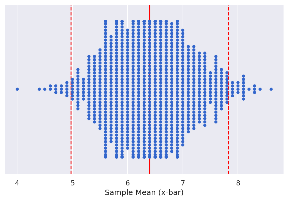
This equation centers the confidence interval around the sampling distribution mean (""), as shown in the figure below.

Confidence interval around the sampling distribution mean ("")
Credit: Eugene Morgan © Penn State is licensed under CC BY-NC-SA 4.0(link is external) [1]
In order to calculate this, we take three key steps in the code, following the development of the bootstrapped sampling distribution.
- Calculate the mean of the bootstrapped sampling distribution using
- Calculate the standard error of the bootstrapped sampling distribution using
- Calculate the 95% confidence interval using the equation above
Below we demonstrate this process.
 Watch It: Video - Introduction to Sampling Distributions (07:12 minutes)
Click here for a transcript.
Credit: © Penn State is licensed under CC BY-NC-SA 4.0 [1]
 Watch It: Video - Confidence Intervals SEmethod (04:58 minutes)
Click here for a transcript.
Credit: © Penn State is licensed under CC BY-NC-SA 4.0 [1]
 Try It: Apply Your Coding Skills in Google Colab
- Click the Google Colab file used in the video here. [2]
- Go to the Colab file and click "File" then "Save a copy in Drive", this will create a new Colab file that you can edit in your own Google Drive account.
- Once you have it saved in your Drive, use the partial code below to calculate and plot the 95% confidence interval.
Note: You must be logged into your PSU Google Workspace in order to access the file.
1 2 3 4 5 6 7 8 9 10 11 12 13 14 15 | # step 1: calculate x barXB = ...# step 2: calculate the standard errorSE = ...# step 3: calculate the 95% Confidence IntervalCI = ...(ggplot(boot_means) + geom_dotplot(...) + geom_vline(aes(xintercept = 7), color = 'blue', size = 1) + geom_errorbarh(...) + geom_point(...)) |
 Assess It: Check Your Knowledge
Knowledge Check
 FAQ
FAQ
(add new questions)