Lesson 9: Multiple Linear Regression

Overview

In the previous lesson, you have learned how to implement simple linear regression, in which you have one response variable and one predictor variable. In this lesson, we will expand what you have learned to multiple linear regression. Here, you will still have a single response variable, but will include multiple explanatory variables in your model.

Learning Outcomes

By the end of this lesson, you should be able to:

choose which variables to include in a multiple regression model
evaluate interactions between variables in a mutiple regression model

Lesson Roadmap

Table listing assignments
Type	Assignment	Location
To Read	Lock et. al. 10.1-10.3	Textbook
To Do	Complete Homework: H11 Multiple Regression Take Quiz 9	Canvas

Questions?

If you prefer to use email:

If you have any questions, please send a message through Canvas. We will check daily to respond. If your question is one that is relevant to the entire class, we may respond to the entire class rather than individually.

If you prefer to use the discussion forums:

If you have questions, please feel free to post them to the General Questions and Discussion forum in Canvas. While you are there, feel free to post your own responses if you, too, are able to help a classmate.

Introduction to Multiple Linear Regression

Read It: Multiple Linear Regression

At its core, multiple linear regression is very similar to simple linear regression. Recall the equation for a simple linear model from Lesson 8:

$Y = β_{1} X + β_{0} + ϵ$

In this equation, we have a single explanatory variable (also known as a predictor), which is denoted with $X$ . To define a multiple linear regression model, we maintain this same basic formula, but add more explanatory variables:

$Y = β_{k} X_{k} + \dots + β_{2} X_{2} + β_{1} X_{1} + β_{0} + ϵ$

Notice that we do not include multiple X values (e.g., $X_1, X_2, \dots, X_k$ ) to indicate the multiple explanatory variables included in the model.

Another similarity between simple linear regression and multiple linear regression are the conditions that need to be met for statistical validity. Recall from Lesson 8, the three conditions for simple linear regression are: (a) linear shape, (b) constant variance, and (c) no outliers. Multiple linear regression has the same conditions, except we test them by plotting the predicted values vs. the residuals, as shown below.

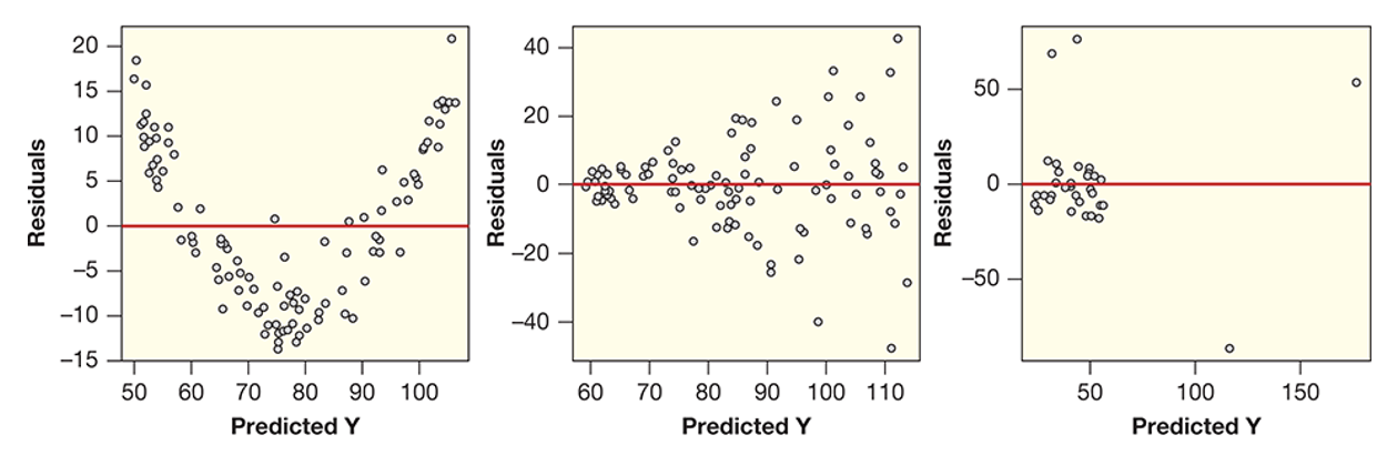
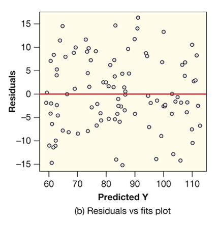
Conditions that break assumptions of the simple linear model

Credit: © Penn State is licensed under CC BY-NC-SA 4.0 [1]

Notice, for example, the curved shape between the predicted Y values and the residuals in Figure (a), this is an indication that there is a nonlinear relationship, which breaks the conditions for multiple linear regression. Likewise, in Figure (b), there is a clear fan or wedge shape between the predicted Y values and the residuals, which breaks the constant variance condition. Finally, in Figure (c), there are clear outliers, which breaks the no outliers condition. Below, we show the ideal plot of predicted Y values vs. residuals, in which none of the conditions are broken.

Ideal plot of predicted Y values vs. residuals

Credit: © Penn State is licensed under CC BY-NC-SA 4.0 [1]

You may have noticed that all of these plots are working with the predicted Y values, rather than the actual values. This means that we can only assess the validity of our multiple linear regression model after we actually implement the model. This is a particular limitation of multiple linear regression, as it can often we a lot of work to build the model, only to find out that it doesn't meet the statistical conditions. Nonetheless, the ability to include additional explanatory variables often improves our model, so it is generally a worthwhile endeavor to spend some time perfecting the multiple linear regression model.

Assess It: Check Your Knowledge

Knowledge Check

Interpreting the Output from Multiple Linear Regression

Read It: Interpreting Output from Multiple Linear Regression

After implementing multiple linear regression in Python, the primary source of interpretation will be the output of the model summary, an example of which is shown below.

Example output of implementing multiple linear regression in Python. This output is critical for interpreting your multiple linear regression model.

Credit: © Penn State is licensed under CC BY-NC-SA 4.0 [1]

There are three key areas to focus on in this plot. The first is the F-statistic and its associated p-value. As in Lesson 8, these values can be used to determine model effectiveness using the F-statistic hypothesis test. For multiple linear regression, however, the alternative hypothesis is slightly different, as shown below.

$F-statistic and p-value for whole model:$

$H_{0} : model is ineffective$

$H_{A} : at least one predictor is effective$

Notice how the alternative tells us that at least one explanatory variable (predictor) is effective, rather than focusing on the model as a whole. To figure out which predictors are effective, you need to look at the lower half of the output, where the coefficients, t-statistic, and associated p-values are listed. These p-values tell you how significant a given explanatory variables, with values < 0.05 (or your chosen significance level) being significant. You can also use these p-values to test the significance of the coefficient using the hypothesis tests below, notice that they are similar to those you learned in Lesson 8 for the hypothesis test for slope.

$t-statistic and p-value for individual predictors:$

$H_{0} : β_{i} = 0$

$H_{A} : β_{i} \neq 0$

Finally, the last piece of critical information in the model summary is the Adjusted R² value. This is the value that you will use to determine the "goodness of fit" for any multiple linear regression models. In particular, the Adjusted R² value accounts for model complexity, as well as the difference between the predicted and actual values. In this sense, adding explanatory variables that don't contribute to the model accuracy can actually reduce your Adjusted R². Mathematically, the Adjusted R² is represented below. You may notice in the above output that the Adjusted R² and regular R² are the same, this happens when there are no insignificant explanatory variables in your model. That being said, it is much more common to have a regular R² that is greater than your Adjusted R².

$R_{a d j}^{2} = 1 - (1 - R^{2}) \frac{n - 1}{n - p}$

Assess It: Check Your Knowledge

Knowledge Check

Implementing Multiple Linear Regression in Python

Read It: Implementing Multiple Linear Regression in Python

In this course we will be implementing multiple linear regression in Python. In particular, we will be using the .ols command from the statsmodels.formula.api library that you learned about in Lesson 8. More information on this command canbe found in the documentation [2]. Below we will demonstrate how to implement multiple linear regression through two videos. The first will set up the data, while the second will focus on the acutal implementation.

Watch It: Video - Data Set Up Visualization (6:50 minutes)

Click here for a transcript.

Credit: © Penn State is licensed under CC BY-NC-SA 4.0 [1]

Watch It: Video - Multiple Linear Regression (9:21 minutes)

Click here for a transcript.

Hello, and welcome to the videos on multiple linear regression. In this lesson we're going to extend what we learned about linear regression to including multiple explanatory variables within our model. So with that, let's go ahead and dive in.

Now in this video, we're mainly going to talk about the data that we're going to use in multiple linear regression, as well as do a preliminary visualization. So I've got several libraries here and I want to point out that we are using the statsmodels.formula.api library. So you learned about this in Lesson 8. This is the way we did linear regression, where we developed a formula using that tilde. We're going to use that here in multiple linear regression code. And so, what the data that we're going to work with throughout this lesson is the Pennsylvania regional greenhouse gas initiative data that we first introduced during the Anova lesson. And so, there are several Excel files that we will use. And I've already got the code set up to read this in. And so we're going to be using the 2030 data. And we're essentially going to be trying to predict the base NOx predict the RGGI NOx pollution levels based off of the base case data.

And so, I'm going to go ahead and run this. And so, as this is going, just a reminder that what this code is doing is its first reading in the Excel files specifying that we're working with sheet 2030. And then we're setting the indices for stuff that we don't want to necessarily add these suffixes to. Then we add the suffixes to differentiate between these different pollutants because we're going to in this code combine them all. So we want to have these different suffixes so that we know which column is for the base case, which is for RGGI, and which is for noaeps. And then finally, I reset the index. And so, if we look at say the first 10 rows, we can see that we've got this ID Latin lawn. We've got so many columns that it's just shortening it for us. And we can come down here, and we've got all of these different stack columns as well. And so we are going to be working with this data set throughout our multiple linear regression lesson. But before we get into multiple linear regression, before we develop the models, the first step is to always visualize the data try to figure out what exactly is going on, gives us an idea about what maybe we want to think about including in our multiple linear regression model. And so, before we can actually run this code, I need to convert the state data into a category so I'm going to say df_merged state.astype category. And this is because the states are actually labeled as numbers. And so, when we read the Excel file in, Python automatically assumes that they're numeric. But for the sake of plotting, we're going to want them to be categorical. And so, then we can use ggplot to do our main plot with our df_merged. And I'm going to set the AES statement inside this main command because our X data is going to be this X, and Y data are going to be the same across all of our plots. And so, we have X is NOx_base Y is NOx_RGGI. And then we can add a point plot. We do still need one extra AES here. We need to set the color equal to the state.

We can add a stat smooth, no need to do an AES here, we can just say the method is LM and then I'm going to show you a little bit of an extra thing with scale_color_brewer. And this is a way that you can very quickly change your color scheme to match one of the preset color_brewer color schemes. So we need to tell it that this is a qualitative data that we're plotting, so categorical data. And then we need to tell it which palette, and these all have set names that you can find online if you just Google Color Brewer. What we're going to be using is set one. And so we can run this, and we can see what we include, just NOx_base and NOx_RGGI. We can see that a lot of the data is going here, but there's this data down here, State 37. This happens to be Pennsylvania. And so our best fit line for just this linear regression isn't too great. It's trying to sort of split the middle between all of these different variables. And it looks like maybe that the state itself is an important explanatory variable and so perhaps when we do get into our multiple linear regression this suggests that maybe we should look into including state as well as NOx_base as our explanatory variable.

Credit: © Penn State is licensed under CC BY-NC-SA 4.0 [1]

Try It: DataCamp - Apply Your Coding Skills

Using the partial code below, implement a multiple linear regression model. Your response variable should be 'y' and the remaining variables should be used as explanatory variables.

1
2
# libraries
import pandas as pd
XXXXXXXXXXXXXXXXXXXXXXXXXXXXXXXXXXXXXXXXXXXXXXXXXX

XXXXXXXXXXXXXXXXXXXXXXXXXXXXXXXXXXXXXXXXXXXXXXXXXX

1/0 0/0

Assess It: Check Your Knowledge

Knowledge Check

Correlation-Based Variable Selection

Read It: Correlation-Based Variable Selection

One way to selet the optimal variables for multiple linear regression is through a correlation analysis. By determining which explanatory variables are most highly correlated with the response, you can get a better idea of important variables, thus implement models with higher adjusted R² values. Below, we demonstrate how to implement this process in Python.

Watch It: Video - Correlation Variable Selection (10:13 minutes)

Click here for a transcript.

Try It: DataCamp - Apply Your Coding Skills

Using the pre-coded variables below. Calculate and print the correlation matrix. Are any of the variables highly correlated? Which would you include in your multiple linear regression model?

1
2
# libraries
import pandas as pd
XXXXXXXXXXXXXXXXXXXXXXXXXXXXXXXXXXXXXXXXXXXXXXXXXX

XXXXXXXXXXXXXXXXXXXXXXXXXXXXXXXXXXXXXXXXXXXXXXXXXX

1/0 0/0

Assess It: Check Your Knowledge

Knowledge Check

Interaction Effects

Read It: Interaction Effects

When developing multiple linear regression models, it is possible to account for interactions between the variables. For example, maybe variable 'x' is not a great predictor of 'y', but the combined effect of 'x' and 'z' is an important predictor. In this case, the interactions can improve the accuracy of our model. In Python, we signify interactions with an asterisk (*) or a colon (:), depending on the type of interaction. The *, for example, indicates that Python should consider both the interaction between two terms and as separate predictors, while the : tells Python that you only want to consider the interaction. Below, we demonstrate the use of these key symbols in Python.

Watch It: Video - Interaction Effects (8:43 minutes)

Click here for a transcript.

Try It: DataCamp - Apply Your Coding Skills

Edit the following code to implement multiple linear regression with interaction effects. Your response variable is 'y' and all other variables can be used as explanatory variables.

1
2
# libraries
import pandas as pd
XXXXXXXXXXXXXXXXXXXXXXXXXXXXXXXXXXXXXXXXXXXXXXXXXX

XXXXXXXXXXXXXXXXXXXXXXXXXXXXXXXXXXXXXXXXXXXXXXXXXX

1/0 0/0

Assess It: Check Your Knowledge

Knowledge Check

Summary and Final Tasks

Summary

Through this lesson, you are now able to use Python to conduct multiple linear regression and interpret those results. You should also be able to select variables to include in your multiple linear regression analysis and explain why those variables were chosen. Finally, you should understand how interaction effects work in multiple linear regression and be able to implement those interactions in Python.

Assess it: Check Your Knowledge Quiz

Reminder - Complete all of the Lesson 9 tasks!

You have reached the end of Lesson 9! Double-check the to-do list on the Lesson 9 Overview page to make sure you have completed all of the activities listed there before you begin Lesson 10.