Lesson 5 Overview

Many major energy projects last a long time. Even those that aren't quite so long-lived are built with the intention that they will operate for many years. Moreover, different energy technology options have different construction and operating costs. The finances of energy projects can be difficult to evaluate for just this reason - they often involve large immediate capital outlays, followed by a stream of revenues (or costs, if the project is uneconomical) over a long period of time. The process of "discounting" is the way that we think about future costs and revenues in terms of decisions that we are forced to make today.

This lesson will be the most mathematically-intensive of the semester. We will learn about the "net present value" as a way of measuring the benefits versus the costs of a long-lived energy project. We will also discuss several other metrics that can be used to evaluate energy projects, and how these metrics are complementary — and can sometimes cause confusion. These metrics represent the “language” of the energy finance community who is responsible to make decisions about financing projects. The market participants use these metrics to compare energy capital investments against each other as well as against other ways to invest capital. For this reason it is very important for the energy professional to master them.

Learning Outcomes

By the end of this lesson, you should be able to:

• Discuss topics related to cost-benefit analysis and decision making
• determine discounted cash flows for an energy project and calculate the net present value based on the pro forma statements
• calculate the internal rate of return for an energy project
• compare the internal rate of return with the project's discount rate, and explain why the internal rate of return will not necessarily lead you to choose the most profitable project
• calculate the levelized cost of energy for an energy project
• develop a solid estimate of the capital costs for your final project

Reading Materials

There are lots of good online resources for understanding net present value. Our primary external resource will be the article Have We Caught Your Interest? [1] This article goes deeper into the math than we will need to, but is nice and concise, and has all of the relevant information on discounting. You should skim this piece before you start in on the lesson material online. You can then return to the reading as a reference.

What is due for Lesson 5?

This lesson will take us one week to complete. Please refer to the Course Calendar in Canvas for specific due dates. Specific directions and grading rubrics for assignment submissions can be found in the Lesson 5 module in Canvas.

• Final Project: Capital Costs

Questions?

If you have any questions, please post them to our Questions? discussion forum (not email). I will not be reviewing these. I encourage you to work as a cohort in that space. If you do require assistance, please reach out to me directly after you have worked with your cohort --- I am always happy to get on a one-on-one call, or even better, with a group of you.

Discounting the Future

Suppose, hypothetically (or perhaps not), that you really like chicken wings. Now, suppose that I were going to give you chicken wings right now. If you are hungry, then you will be happy since I am giving you something that: (a) sates your hunger; and (b) tastes yummy. And I'm giving them to you right now. No waiting.

Now, suppose that I told you that I would give you the same chicken wings, but one hour from now. Assume that I just bought the chicken wings, and I'm going to let them sit in my car for the next hour. How happy are you right now about the prospect of getting these particular chicken wings in one hour? Well, maybe they will get a little bit cold, and maybe in the meantime you would eat something else to satisfy your hunger, but in one hour they will seem like pretty much the same chicken wings.

Now, suppose that I buy chicken wings right now, but I'm going to wait until tomorrow (24 hours from now) to give it to you. How happy are you right now about these chicken wings that you will get tomorrow? Probably less so - first of all, you are hungry now. Sure, you will be hungry again tomorrow, but will those chicken wings taste quite as good after sitting in my car for a day? Probably not.

Now, (really, we're almost to the point), suppose that I buy chicken wings right now, but I'm going to wait six months to give them to you. How happy are you right now about these chicken wings that will sit in my car for six months before being given to you? What will happen to those chicken wings between now and six months from now? Will they still even be recognizable as chicken wings? I won't even mention the special sauce…

On the other hand, they’re chicken wings. Why is it any different to you whether you get it now, a day from now, or six months from now? Basically, there are three reasons:

1. Physical depreciation: After six months or even maybe one day, those chicken wings won't be as tasty as right now because they are a perishable product. This is the same thing as "inflation" when we talk about money. Inflation depreciates the purchasing power of a fixed quantity of money.
2. Impatience: If you are hungry, then you want the chicken wings right now, not sometime in the future. Even if I told you that I would buy you fresh chicken wings six months from now, that's not a very meaningful promise at this moment in time. Remember, you are hungry now!!!
3. Opportunity cost: If I make you wait an hour for the chicken wings, then you have to be hungry for an hour. On the other hand, you could also eat something else right now instead of having to wait an hour for the chicken wings. Whatever you chose not to eat right now in order to wait for the chicken wings reflects an "opportunity cost" that you have foregone.

Evidently, the same chicken wings (whether they will be fresh or had sat in my car for some unfathomable period of time) are worth less to you if you get them in the future than if you get them now. The process of measuring how fast those chicken wings lose value to you, relative to their value right now, is called discounting. The "discount rate" measures how quickly or slowly something loses value over time. A high discount rate means that something loses value quickly relative to its value at the present time. A low discount rate means that something loses value slowly relative to its value at the present time. A discount rate of zero means that something does not lose any value over time - it's worth just as much in a day, week, year, decade, or century as it is right now. Remember: the discount rate measures how quickly something loses value over time. It does not measure whether something is valuable or not valuable in absolute terms.

The particular method of discounting that we will cover in this lesson is known as "exponential discounting" because of the assumption that something loses value at a constant rate (percent per year) over time. An alternative discounting method that we won't cover, but you can look at in your spare time, is known as "hyperbolic discounting." Wikipedia has a nice article on hyperbolic discounting. [2]

Before we can dive in, we need some terminology:

• PV = Present Value, i.e., the value of something today (or what something in the future is worth to you in today's terms). The present value is sometimes called the "principal" (as in the case of a loan).
• FV(t) = Future Value of something at time t. This time t is usually defined relative to the present day, and usually (but not always, so be careful) in years. So, t = 5 would mean five years from this year.
• r = Discount rate, in percentage terms. This is also usually defined on an annual basis, but does not need to be. So, a value of r = 0.05 would be a discount rate of 5% per year. In the case of a loan, r is equivalent to the annual interest rate.

Suppose that you were to put some amount PV in a simple investment vehicle, like a bank account, that paid back your money plus a rate of return r every year. The future value of that amount in one year (t=1) would be:

$$FV(1)=PV(1+r)=PV+r\times PV$$

If you kept your money in the account for another year, in that second year you would earn a rate of return r on all the money that was in your account the first year:

$$FV(2)=[PV+r\times PV]\times (1+r)=PV{(1+r)}^2$$

Note that you have effectively earned interest in the second year on the interest that you earned in the first year. This phenomenon is called "compounding." Since interest is calculated once per year in this model, we call this "annual compounding."

There is a detailed section in the "Have We Caught Your Interest" reading that discusses compounding at intervals more frequent than annually, all the way up to continuous compounding. Please read this section carefully, although in this class we will use annual compounding almost exclusively.

Going back to our little bank account, more generally, in year t the future value of the investment that you make today is:

$$FV(t)=PV{(1+r)}^t$$

This equation is an indifference condition - it says that you would be equally happy getting some amount of money PV right now, or $FV(t)=PV{(1+r)}^t$ if you had to wait t years to get your money. The factor ${(1+r)}^t$ just measures your opportunity cost for having to wait t years.

Now, we will flip the equation on its head. Suppose that you were promised some amount of money FV(t) in year t, sometime in the future. What is that promise of future wealth worth to you today? In other words, what would you need to be paid today in order to be equally happy between getting money today and getting the amount FV(t) in the future? We can find this by manipulating the previous equation to solve for PV. Dividing both sides by $1/{(1+r)}^t$, we get:

$$PV=\frac{FV(t)}{{(1+r)}^t}$$

Assuming that r is greater than zero, this means that the value in the present of some amount of money that you are going to get in the future is lower than the face value of that amount of money. In other words, you would be willing to accept less money right now in exchange for not needing to wait to get it. This is sensible, if you think about it. First, people are impatient. Second, there is an opportunity cost to waiting. If I got some amount PV right now (rather than some larger amount FV(t) in the future), then I could take that amount PV and do something with it that might increase its worth t years from now.

The term $1/{(1+r)}^t$ is known as the "discount factor" and it measures how quickly something has declined in value between now and t periods from now.

Here are two examples that illustrate the mechanics of discounting.

Example #1: Suppose that r = 0.04 (4%), t=20. The discount factor is equal to:

$$1/{(1.04)}^{20}=0.46$$

Thus, PV = 0.46×FV. What this says is that the present value is less than half of the future value after 20 years.

Example #2: Now suppose that t = 100. The discount factor is equal to:

$$1/{(1.04)}^{100}=0.02$$

Thus, PV = 0.02×FV. What this says is that the present value is only 2% of the future value.

These two examples, although simple and without much context, illustrate two important properties of exponential discounting. First, at any positive discount rate, if you go far enough into the future, then the future is worthless, and you would never consider it when making decisions in the present. Second, the higher the discount rate, the faster the future becomes worthless relative to the present. Remember that the discount rate does not determine whether one thing will be worth more or less in the future than another thing. It only measures the value of something in the future relative to that same thing in the present (like chicken wings six months from now versus the exact same chicken wings today).

There is almost nothing that puts students to sleep faster than the discount rate. Frankly, it's a dry topic. But the discount rate is actually front and center - in some ways, much more so than any science - in the debate over climate change and how societies should respond. The reason for the controversy is simple - if the worst impacts of climate change are going to be felt even two generations from now, then unless we use a discount rate of zero or near zero (meaning that we value the future exactly as much as the present) it is difficult to justify large and costly climate-related interventions in the present, in order to yield substantial benefits far in the future. But such a low discount rate flies in the face of what economists actually know about preferences that people seem to have for happiness now versus happiness (or wealth) in the future. If you are really interested in this topic from the perspective of climate change, Grist has a nice piece [3] (from a while ago). Since our focus in this course is on commodity markets and business decisions, we'll find (in the next couple of lessons) that there is a logical way to determine the "right" discount rate for those types of decisions.

Project Decision Metrics: Net Present Value

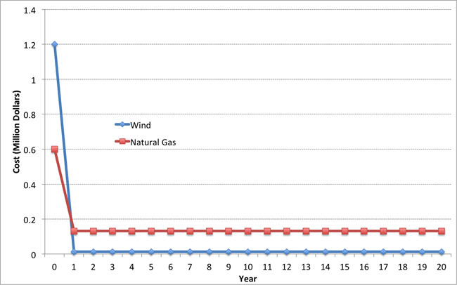
Suppose that you were an electric utility considering two potential generation investment opportunities: A natural gas-fired generator with a capital cost of 600 dollars per kW and operating costs of 50 dollars per MWh, or a wind farm with a capital cost of 1,200 dollars per kW and operating costs of 5 dollars per MWh. For the purposes of this example, assume that either power plant could meet the same reliability goals that your utility had. But your regulator wants you to minimize economic costs to consumers. Which should you pick?

This is a difficult choice because it involves tradeoffs over time. The natural gas generator has a low up-front cost but a higher operating cost. The wind generator has a higher up-front cost but a very low operating cost, because fuel from the wind is free (at the margin). This tradeoff is shown visually in Figure 5.1, for a 1 MW natural gas and wind power plant — for the sake of comparison, we assume that each of the plants operates 30% of the time, so each produces 1 MW × 8,760 × 0.3 = 2,628 MWh per year.

This 30% figure is called the capacity factor, and it measures how much electricity a power plant produces in a year versus how much it could produce each year if it operated all the time at 100% capacity.

Capacity Factor = (Annual Production) ÷ (Capacity × 8,760 hours per year).

Figure 5.1 illustrates the tradeoff but doesn't say much about which decision you should make. Part of the problem is that by investing in the wind turbine, you are accepting a high cost right now in exchange for a stream of operating cost savings in the future. Is this stream of operating cost savings worth it?

One of the most frequently-used metrics to compare projects with different capital and operating cost streams is the net present value, which incorporates the present discounted value of all project costs and revenues.

Figure 5.1: Capital and operating costs for a 1 MW natural gas and wind power plants over a 20-year operating horizon.

The net present value (NPV) is defined by two terms: the present discounted value of costs and the present discounted value of revenues. If we let B_t be the (undiscounted) revenues (benefits) of some project during year t and we let C_t be the (undiscounted) costs of the same project during year t, then we can calculate the NPV as follows:

$\text{Present discounted benefits}=PDB={\displaystyle \sum _{t=0}^T\frac{B_t}{{(1+r)}^t}}$

$\text{Present discounted costs}=PDC={\displaystyle \sum _{t=0}^T\frac{C_t}{{(1+r)}^t}}$ /p>

$\text{Net present value}=NPV=PDB-PDC={\displaystyle \sum _{t=0}^T\frac{(B_t-C_t)}{{(1+r)}^t}}$

In the equations, T is the time horizon for the project and r is the discount rate. If the net present value of a project is greater than zero, then the project is said to break even or be "feasible" in present discounted value terms. If you are in a position where you are evaluating multiple alternatives, you would normally want to choose the alternative with the highest net present value.

Sometimes, we will be interested in the net present value of a project as of some year prior to T. We will call this the "Cumulative NPV" as of year X. Mathematically, this is defined as:

$\text{Cumulative NPV}={\displaystyle \sum _{t=0}^X\frac{(B_t-C_t)}{{(1+r)}^t}}$

Where X is some number smaller than T.

To illustrate, let's go back to one of our examples from earlier in this lesson. Our wind power plant had a capital cost of $1.2 million and annual operations costs of $13,140. Suppose that it had annual revenues of $100,000 and faced a discount rate of 10% per year. Each year, it thus has annual profits of $86,860.

Assuming that all of the capital costs were incurred in Year 0 and the plant began operating in Year 1, the present discounted value of each of the first three years of operation would be:

The Cumulative NPV for the first three years would be:

Calculating NPV is reasonably straightforward in a spreadsheet program such as Excel. There are two functions in Excel, PV and NPV, that will calculate net present value for you. The difference between the PV and NPV functions is that the PV function assumes that you have the same profits in each period (as in our example above), while the NPV function does not make this assumption.

The video below shows an example of evaluating NPV using Excel. The example in the video is our natural gas plant from the previous lesson. Registered students can access the Excel file discussed in the video in Canvas.

Video: NPV Example Video (15:19)

There are two special cases where calculating the NPV is especially simple - the "annuity" and the "perpetuity." When a project's annual cash flow is the same in each year, not unlike a fixed-rate mortgage, we refer to this type of project as having an annuity structure. In this case, because the cash flow is the same each year, the summation term in the NPV can be greatly simplified. The formula for the present value of an annuity is shown below; if you are interested you can find the derivation in the reading accompanying this lesson.

$\text{Present Value of Annuity}=a\times \left(\frac{{(1+r)}^T-1}{r\times {(1+r)}^T}\right)$

where a is the annual cash flow. To illustrate this, let's calculate the present value of the wind power plant over a three year operating time horizon (T=3), using the annuity formula. One of the tricks here is that you need to take the Year 0 cash flow (the 1.2 million dollars capital cost) outside of the formula.

$\text{Present Value }=-\$1.2million+86,860\times \left(\frac{{(1.1)}^3-1}{0.1\times {(1.1)}^3}\right)=-\$983,992$ , which is just what we got using the NPV formula.

If an annuity involves identical payments over a long period of time (tens of decades, for example), we can approximate the NPV of the annuity using an extremely simple formula called a perpetuity. If we take the annuity formula and let T get really really large (tending towards infinity) then the "-1" term from the numerator becomes meaningless relative to the ${(1+r)}^T$ term, and the present value becomes:

$\text{Present value of a perpetuity}=a/r$ .

As a rule of thumb, if the annuity lasts longer than 30 years, you can probably approximate the present value reasonably well using the perpetuity formula.

Project Decision Metrics: Internal Rate of Return

The internal rate of return (IRR) is one of the most frequently used metrics for assessing investment opportunities. The IRR is defined as the discount rate for which the NPV of a project is zero. The definition is simple, but the IRR is generally impossible to calculate without a computer.

If you use Excel, there is a built-in IRR function that will calculate the IRR for you, given a stream of costs and benefits over time.

Unlike the NPV, which takes units of dollars, the IRR is given in percentage terms (% discount rate per year such that the project NPV is zero). We call this a "yield" measure of return. This can be very convenient when comparing different types of projects. In many cases, the project with the largest yield (i.e., highest IRR) will be the most desirable. The IRR can also be compared to the investor's "hurdle rate," which is the lowest return that an investor is willing to accept before putting money into a project. Energy projects that will sell their output into competitive markets often need a yield higher than, say, a 15% hurdle rate over a five-year period. This means that the project's return on investment must be at least 15%, and that this yield must be realized within five years. If the IRR of a prospective project is higher than the hurdle rate, the project could be considered attractive to an investor.

While the IRR is often an appropriate measure for determining whether an individual project is worthwhile, there are three cases where IRR may not be very useful or may yield misleading information.

First, if a project has some years with positive cash flow and some years with negative cash flow (an example is on the power plant pro forma from the previous lesson), then it is possible that the IRR may have multiple values. Mathematically, this arises because a high-order polynomial equation may have multiple (non-unique) roots. As a simple example, if the cash flows for a project over three years are -$10, $21 and -$11, then there would be two IRRs for this potential project: 0% (because it just breaks even) and 10%.

Second, if a project has negative total undiscounted cash flows over its lifetime, then the IRR is mathematically undefined.

Third, it is possible that the project with the highest IRR may not be the project with the largest NPV. In other words, some types of projects can see their NPV increase when the discount rate goes up, which is the opposite of what we would expect to happen. This situation occurs when projects have large cash outlays at their end-of-life. Nuclear power plants are a good example — at the end of a nuclear power plant's life (at least in most developed countries), the owner must pay a large amount to have the plant decommissioned. If the discount rate used by the plant's owner is low, this increases the contribution of that end-of-life cash outlay to the NPV. If the discount rate used by the plant's owner is high, then that end-of-life cash outlay is not very important, in present value terms.

Here is a simple example. Suppose that a hypothetical investment requires a $5 cash outlay in Year 0, then earns $5 per year in Years 1 through 5. In Year 6, the project requires a cash outlay of $22.50. As an exercise, calculate the NPV assuming a discount rate of 10% per year and 5% per year. You should get NPVs of $1.25 and -$0.14.

Project Decision Metrics: Levelized Cost of Energy (LCOE)

Let's return to our wind power and natural gas power plant example from earlier in this lesson. Suppose that both power plants were selling electricity into the same deregulated generation market and both had the same expected operational life. Which plant would be more profitable? Since both plants would be facing the same market price for the electricity that they sell, the more profitable plant would be the one that had the lower average cost per Megawatt-hour of electricity over its entire lifetime.

The Levelized Cost of Energy (LCOE) can be used to help evaluate problems like this one, and is one of the most commonly used metrics for assessing the financial viability of energy projects. It is used particularly often in situations like the one we just discussed - comparing the lifetime costs of different technologies for electric power generation. The LCOE can, however, be applied to other energy projects as well (like oil and gas wells, or refineries).

The LCOE is defined as the energy price ($ per unit of energy output) for which the Net Present Value of the investment is zero.

The LCOE is thus the average revenue per unit of energy output (so this would be $/MWh for a power plant, or $/barrel for an oil well, for example) over a project's lifetime such that the plant breaks even. The LCOE is sometimes called the Unit Technical Cost (UTC). It represents the lifetime average cost of energy for a specific project.

We will now get into the mathematics of calculating the LCOE. We will first present the most generic LCOE formula, and then we will discuss some simplifications of the formula.

LCOE is defined as the solution to the equation:

$${\displaystyle \sum _{t=0}^T\frac{C_t+M_t}{{(1+r)}^t}={\displaystyle \sum _{t=0}^T\frac{LCOE\times Q_t}{{(1+r)}^t}=LCOE{\displaystyle \sum _{t=0}^T\frac{Q_t}{{(1+r)}^t}}}}$$

where C_t represents all capital costs incurred in year t (these may be zero except during the first few years of the project); M_t represents all operational costs incurred in year t, and Q_t represents the total output of the project in year t. The term C_t + M_t represents the annual costs of the project (which may include payments on capital, fuel, labor, land leases and so forth). The term Q_t represents the annual energy output of the plant.

Note that if all capital costs are incurred in year zero, then the term C_t factors out of the LCOE equation. In this case, you will sometimes see the capital cost term referred to as "Total Installed Cost" (TIC) or "Overnight Cost" (OC). In this case, we write the LCOE equation as:

$${\displaystyle \sum _{t=0}^T\frac{M_t}{{(1+r)}^t}+TIC={\displaystyle \sum _{t=0}^T\frac{LCOE\times Q_t}{{(1+r)}^t}=LCOE{\displaystyle \sum _{t=0}^T\frac{Q_t}{{(1+r)}^t}}}}$$

In some other contexts (for those of you taking AE 878 through the RESS program, for example), you may see the discount rate r referred to as the "Weighted Average Cost of Capital" (WACC). We will devote an entire lesson later in the term to the relationship between the discount rate and the WACC (sneak preview: if the entity making the project investment is a for-profit entity, then the discount rate and WACC should be the same thing), and methods for calculating what the WACC should be.

We can thus solve for LCOE as:

$$LCOE=\frac{{\displaystyle \sum _{t=0}^T\frac{C_t+M_t}{{(1+r)}^t}}}{{\displaystyle \sum _{t=0}^T\frac{Q_t}{{(1+r)}^t}}}$$

There are a couple of ways to make this calculation easier. Often times when evaluating prospective energy projects we make two assumptions:

• First, annual output of the project is constant in each year.
• Second, the variable cost of production per unit of output is constant each year.

In this case, the Q and M terms from the LCOE equation are the same in each year, and we can write the LCOE as the sum of two terms:

1. Levelized Fixed Cost (LFC), which calculates the average payment required to "amortize" or pay off capital costs over T years.
2. Levelized Variable Cost (LVC), which calculates the average payment required to cover per-unit operational costs.

If the variable cost of production (this would include fuel, labor and any variable operations/maintenance costs) don't change, then the LVC is just equal to this total variable cost per unit of output. Referencing the LCOE equations above, LVC would just be equal to M ÷ Q. (The LVC may also just be given in the problem statement, as in the examples below.)

Calculating LFC is a little bit more complicated. Assume that the project involves a discount rate r; the life of the project is T years; and the capital costs are paid in one lump sum TIC at the beginning of the project. LFC solves the equation:

$$TIC={\displaystyle \sum _{t=0}^T\frac{LFC}{{(1+r)}^t}}/Q$$

which we can rewrite as:

$$LFC=\frac{TIC}{{\displaystyle \sum _{t=0}^T\frac{1}{{(1+r)}^t}}}/Q$$

Using some mathematics of finite sums (if you are really curious, Wikipedia has a detailed article on the "geometric series [5]," which describes the denominator of the LFC equation), since r is less than one, we can rewrite the denominator as $\frac{1-{(1+r)}^{-T}}{r}$

Thus,

$$LFC=\frac{TIC}{\frac{1-{(1+r)}^{-T}}{r}}/Q=\frac{TIC\times r}{1-{(1+r)}^{-T}}/Q$$

and finally, we have our expression for LCOE:

$$LCOE=LFC+LVC=\left(\frac{TIC\times r}{1-{(1+r)}^{-T}}/Q\right)+LVC$$

Along these same lines, another (less messy) way to write the LCOE when output and variable costs are constant over time uses the "fixed charge rate" (FCR). The FCR is just the fraction of the Total Installed Cost (TIC) that must be set aside each year to retire capital costs (which includes interest on debt, return on equity and so forth - we'll discuss these in more detail in future lessons). Thus, TIC × FCR is the annuity payment (the sum of principal plus interest payments, like you would have with a home mortgage or a college loan) needed to pay off the investment's capital cost. The FCR is calculated as:

$$FCR=\frac{r}{{(r+1)}^T-1}+r$$

(You may see or have seen the FCR equation written with the WACC rather than the discount rate r. Remember that, for our purposes, there is really no difference between the two.)

Using the fixed charge rate, the LCOE can be written as:

$$LCOE=\left(\frac{TIC}{Q}\times FCR\right)+\frac{M}{Q}$$

In this simpler version of the LCOE equation, note that the first term $\left(\frac{TIC}{Q}\times FCR\right)$ is just the Levelized Fixed Cost (LFC) and the second term (M/Q) is just the Levelized Variable Cost (LVC).

Here is an example: Suppose that a power plant costs $10 billion to build and has an expected life of 30 years. The variable cost of producing one MWh of electricity is $20. It will operate 24 hours a day, 360 days a year at a capacity of 1000 MW. (Note: to get output, multiply capacity and hours of operation over the plant's life). What is the levelized cost of energy if the interest rate is 5%?

Here is the answer: First, we calculate the total amount of electricity produced annually:

(360 days per year) × (24 hours per day) × 1000 MW=8.64 million MWh per year.

This is Q in our LCOE formula. LVC is equal to $20 per MWh. So, we calculate LCOE as:

$$LCOE=\left(\frac{TIC\times r}{1-{(1+r)}^{-T}}/Q\right)+LVC$$

$$LCOE=\left(\frac{\$10bil\times 0.05}{1-{(1+0.05)}^{-30}}/8.64mil\right)+20$$

$$=\$75.29/MWh+\$20/MWh=\$95.29MWh$$

As an exercise for yourself, calculate the LCOE for the natural gas power plant and the wind power plant that we laid out earlier in this lesson. As a reminder, the wind plant has a capital cost of $1.2 million and a variable cost of $5/MWh. The natural gas plant has a capital cost of $600,000 and a variable cost of $50/MWh. Each plant produces 2,628 MWh per year. Assume a 10% annual discount rate and a 20-year life for each project. You should find that the wind plant has LCOE = $58.63/MWh and the gas plant has LCOE = $76.82 per MWh.

The LCOE can be used to compare energy projects to prevailing market prices. If the market price is higher than the LCOE, then the margin per unit of output is positive (Market price - LCOE is greater than zero) and the project should be profitable. If the market price is lower than the LCOE, then the project will have negative margins and will not be profitable. There are some pitfalls to using LCOE in this way to evaluate variable renewables like wind and solar, since the LCOE is often compared to the average electricity price. If you think about it, this comparison is biased against solar and biased towards wind because solar is more likely to be producing electricity during the daytime (when prices are high) and wind is more likely to be producing electricity during the nighttime (when prices are usually low). A more consistent approach, which is just as relevant for fossil-fired power plants as for renewables, would be to compare the LCOE to the average price when you would expect the power plant to be generating electricity.

Lesson 5 Summary and Final Tasks

Summary

Most energy projects involve large capital outlays at the beginning of project life, followed by a stream of costs and benefits during the project's years in operation. (Some types of energy projects would end their lives with large capital outlays as well, to handle decommissioning or other environmental issues.) Since waiting to enjoy future benefits from an energy project involves opportunity costs, a dollar of benefit in the future is worth less than a dollar of benefit now. These streams of future costs and benefits need to be expressed in terms of value at the time that the project decision is being considered or initiated. This process is called "discounting."

Project alternatives may have different capital and operating costs, even if they ultimately produce the same product. Electricity is probably the best example of this - power plants generally exhibit a tradeoff between capital and operating cost. We developed three different but related metrics to evaluate stand-alone projects and to compare the relative economic merits of project alternatives. The net present value will tell you which project will be the most profitable in absolute present-value dollar terms. The internal rate of return can be useful in comparing percentage returns or "yields" on different projects, or for checking whether a proposed investment exceeds the hurdle rate set by an individual investor or company. The internal rate of return cannot, however, always identify the most profitable project. The levelized cost of energy will tell you the average revenue per unit of output required for a proposed investment to break even, in present value terms. Levelized costs are often compared to prevailing market prices to estimate margins, but this comparison needs to be done with care if energy projects are not expected to run around the clock.

Reminder - Complete all of the Lesson 5 tasks!

You have reached the end of Lesson 5! Double-check the What is Due for Lesson 5? list on the first page of this lesson to make sure you have completed all of the activities listed there before you begin Lesson 6.