Overview

In Lesson 1, we learned that the main function and purpose of the solar energy systems is to convert sun radiation - i.e., light or heat - into electricity. However, the efficiency of such conversion is not very high. One way to make many known solar technologies feasible with respect to their efficiency, total output, environmental impact, and cost is to concentrate the incoming radiation. Concentration of light will be the main topic of Lesson 2.

Sunlight is a practically inexhaustible natural resource which is also universally available. However, one of the disadvantages or difficulties related to its utilization is a relative low density of the solar flux. To generate sufficient power to meet demands of large populated zones, a vast area should be covered by solar collectors, and a significant amount of materials and resources should be spent on production and service of those collectors. This expense raises a question about economic viability of solar and initiates the search for ways to increase the sunlight conversion efficiency one way or the other. Generally, there are two ways to solve the problem - to improve the conversion device (intrinsic factor) or to increase the input flux (extrinsic factor). While the first avenue is subject to energy engineering research and innovation (e.g., developing new types of photovoltaic materials and devices), the second option - concentration of the incident solar flux - is already widely implemented. This lesson presents basic concepts for sunlight concentration and discusses typical optical geometries common in utility scale solar plants. This material provides background for further discussion of such technologies as concentrating solar power (CSP) or concentrating photovoltaics (CPV) later in this course.

Learning Objectives

By the end of this lesson, you should be able to:

1. understand the physical principles of light concentration;
2. list the main types of concentration systems used for utility scale solar facilities;
3. calculate parameters of the typical light concentrating systems (CPC, parabolic concentrators).

2.1 Available Solar Radiation and How It Is Measured

Before talking about concentration of light for practical purposes, it would be good for us to review what kinds of natural radiation are available to us and how that radiation is characterized and measured.

Solar Constant

The fraction of the energy flux emitted by the sun and intercepted by the earth is characterized by the solar constant. The solar constant is defined as essentially the measure of the solar energy flux density perpendicular to the ray direction per unit area per unit of time. It is most precisely measured by satellites outside the earth atmosphere. The solar constant is currently estimated at 1361 W/m² [cited from Kopp and Lean, 2011 [1]]. This number actually varies by 3% because the orbit of the earth is elliptical, and the distance from the sun varies over the course of the year. Some small variation of the solar constant is also possible due to changes in Sun's luminosity. This measured value includes all types of radiation, a substantial fraction of which is lost as the light passes through the atmosphere [IPS - Radio and Space Services].

Transformations in the Atmosphere

As the solar radiation passes through the atmosphere, it gets absorbed, scattered, reflected, or transmitted. All these processes result in reduction of the energy flux density. Actually, the solar flux density is reduced by about 30% compared to extraterrestrial radiation flux on a sunny day and is reduced by as much as 90% on a cloudy day. The following main losses should be noted:

• absorbed by particles and molecules in the atmosphere - 10-30%
• reflected and scattered back to space - 2-11%
• scattered to earth (direct radiation becomes diffuse) - 5-26% [Stine and Harrigan, 1986]

As a result, the direct radiation reaching the earth surface (or a device installed on the earth surface) never exceeds 83% of the original extraterrestrial energy flux. This radiation that comes directly from the solar disk is defined as beam radiation. The scattered and reflected radiation that is sent to the earth surface from all directions (reflected from other bodies, molecules, particles, droplets, etc.) is defined as diffuse radiation. The sum of the beam and diffuse components is defined as total (or global) radiation.

It is important for us to differentiate between the beam radiation and diffuse radiation when talking about solar concentration in this lesson, because the beam radiation can be concentrated, while the diffuse radiation, in many cases, cannot. For that matter, the solar systems utilizing concentrating collectors will work best in sunny locations and may be not feasible in those with a lot of weather variability and clouds. 

Solar Radiation Metrics

Consider the following metrics commonly used to report the solar resource (irradiance) data. These values can be determined from the field measurements or from empirical correlations.  

Theoretically, these three metrics are interrelated:

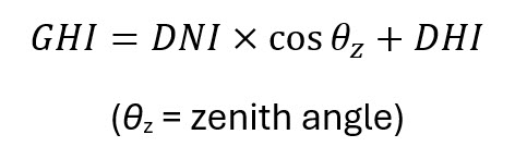
However, in practice, field measurements may somewhat deviate from this relationship.

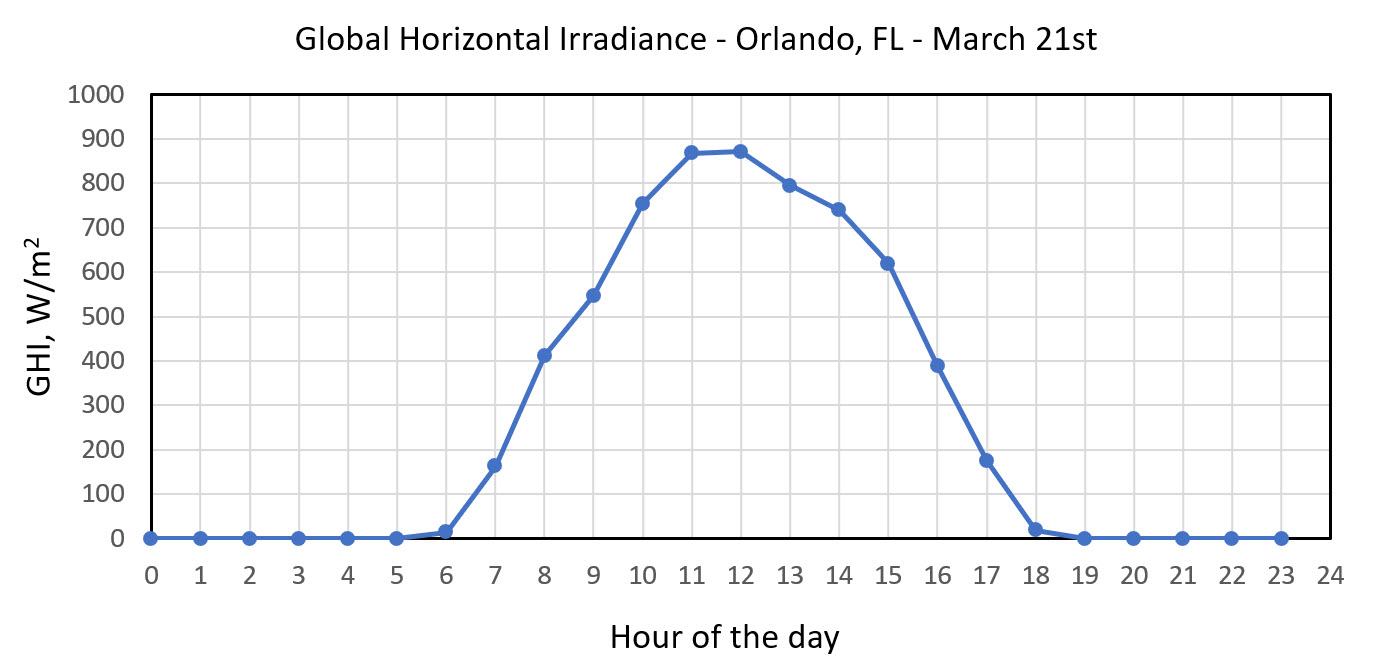
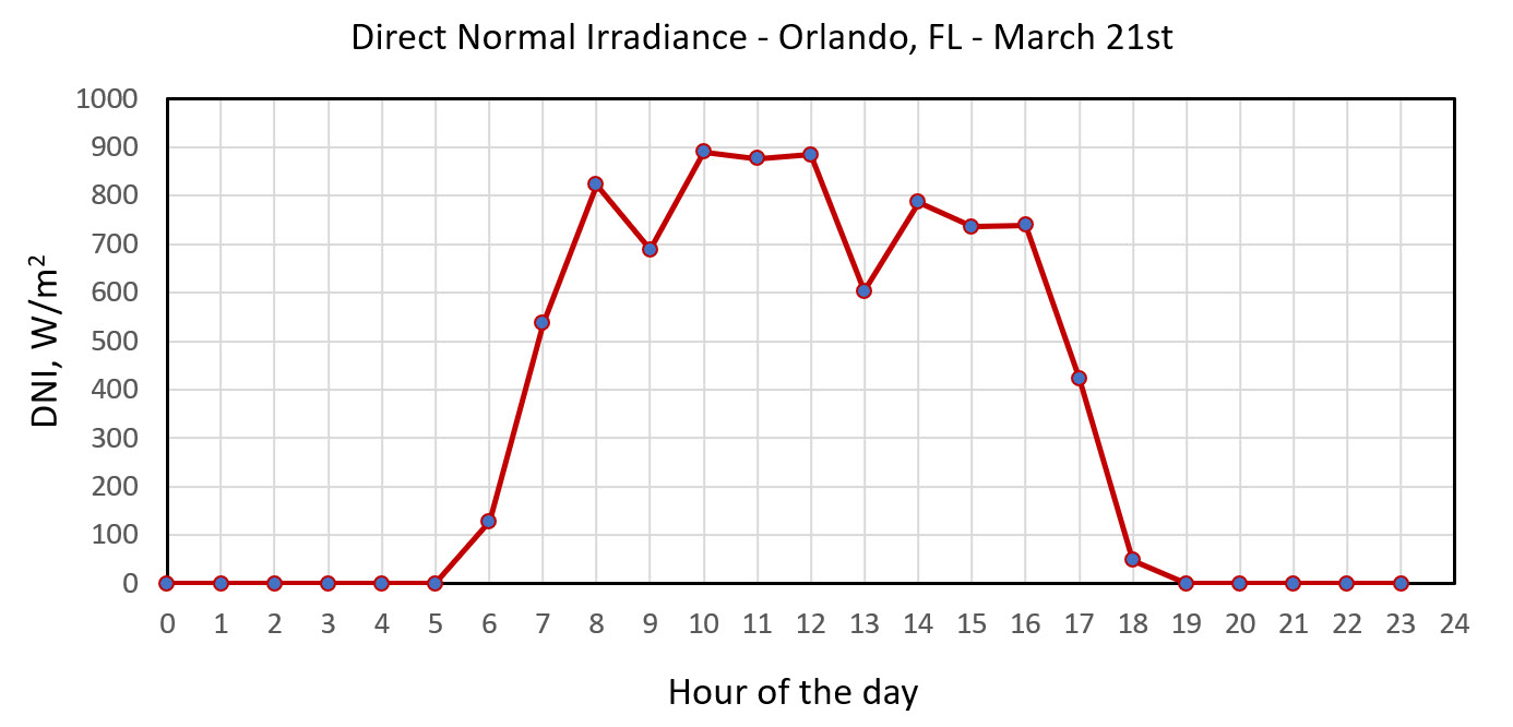
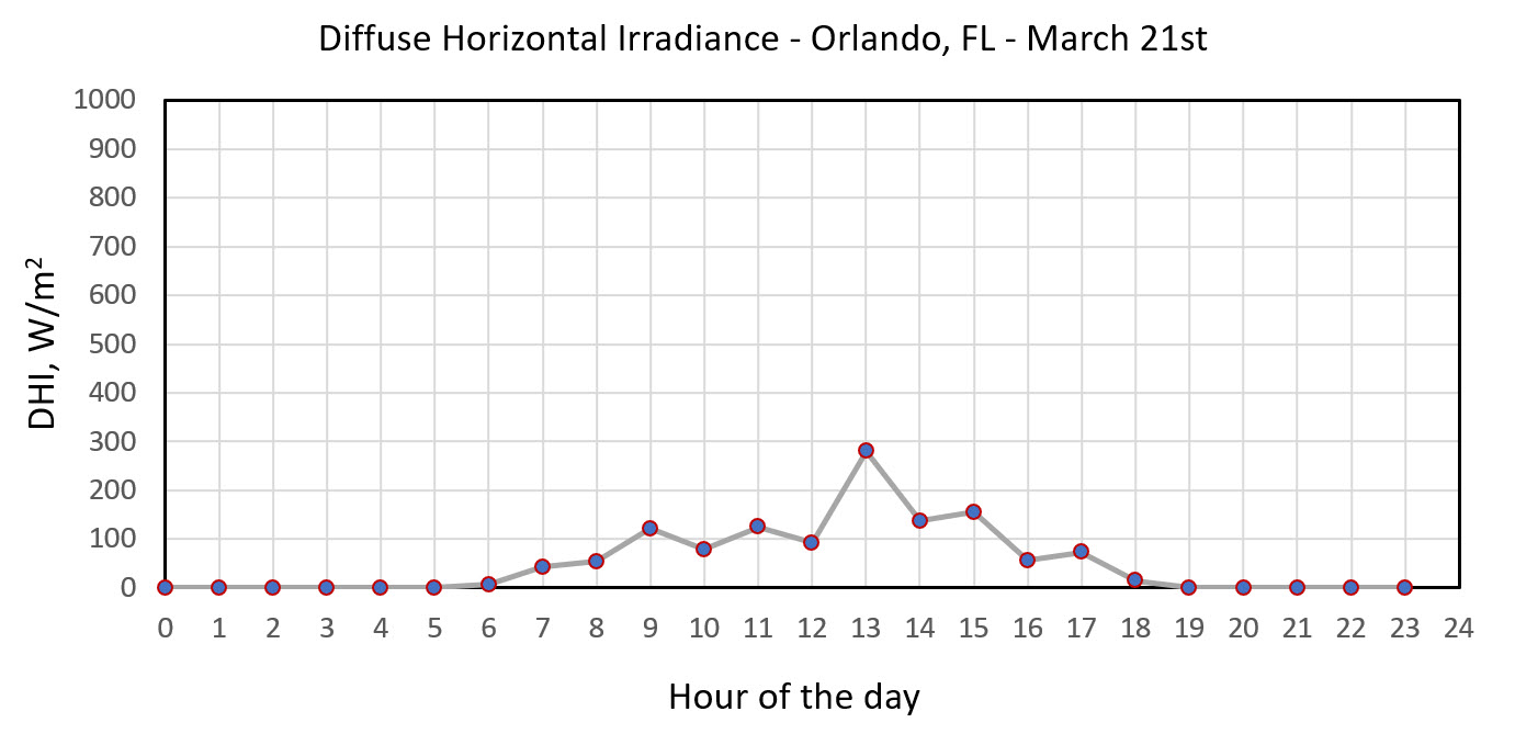
A typical solar resource data file (Typical Meteorological Year or TMY) would include all of these metrics measured for a specific location for each hour for each day in a year. Note that these values (measured in W/m²) indicate the instantaneous solar flux, which of course will vary during the day. In the morning and in the evening, the irradiance will be lower, but it will often reach its peak around solar noon. If there are clouds or other weather phenomena, the irradiance will temporarily drop.

The plots below give you an example of such variance. The GHI, DNI, and DHI data are plotted for the day of March 21st (equinox) in Orlando, FL. While it seemed to be a relatively sunny day (the beam component evidently dominates over diffuse, reaching ~900 W/m²), there are some minor interruptions (possibly from clouds) to this profile.

Daily profiles for different types of solar radiation in Orlando, FL, on March 21 - extracted from the TMY weather file. 

Credit: Mark Fedkin

The TMY files with all these metrics given for each day for different locations around the globe are publicly available from the NSRDB database. 

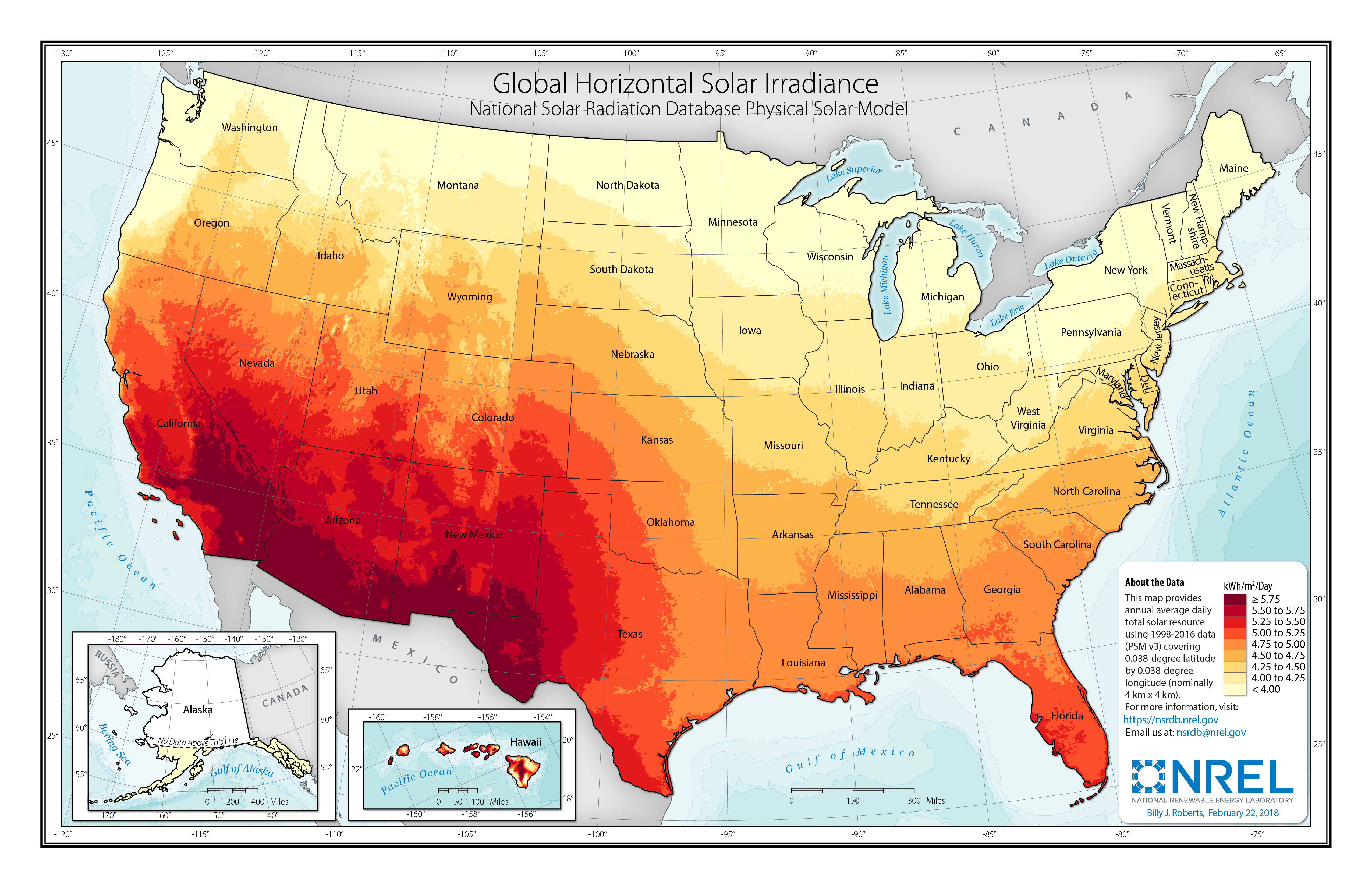
Solar Maps

The GHI data are also used to generate solar resource maps. However, the instantaneous values of global irradiance are not best for mapping due to their continuous variability. Instead, GHI are integrated to determine the daily average irradiation (total energy from the sky).

Look again at the GHI plot (blue curve above) – essentially, this total daily energy will be equal to the area under the irradiance curve! This total daily irradiation value (measured in kWh/m²/day) can be better related to the total energy converted and delivered by your solar system. In a practical sense, it is a more intuitive metric to map.

Also, let’s not forget the seasonal variations. The solar daily irradiation will be understandably higher during summer months and lower during winter months. Hence, the map below is based on the annual average values of daily irradiation.

Solar Irradiation Map for the U.S. in terms of annual average daily GHI (kWh/m²/day)

Sengupta, M., Y. Xie, A. Lopez, A. Habte, G. Maclaurin, and J. Shelby. 2018. "The National Solar Radiation Data Base (NSRDB)." Renewable and Sustainable Energy Reviews 89 (June): 51-60.

National Renewable Energy Laboratory [3]

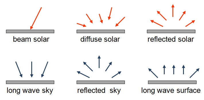
Short-Wave and Long-Wave

Short-wave radiation, in the wavelength range from 0.3 to 3 μm, comes directly from the sun. It includes both beam and diffuse components.

Long-wave radiation, with wavelength 3 μm or longer, originates from the sources at near-ambient temperatures - atmosphere, earth surface, light collectors, other bodies.

The solar radiation reaching the earth is highly variable and depends on the state of the atmosphere at a specific locale. Two atmospheric processes can significantly affect the incident irradiation: scattering and absorption.

Scattering is caused by interaction of the radiation with molecules, water, and dust particles in the air. How much light is scattered depends on the number of particles in the atmosphere, particle size, and the total air mass the radiation comes through.

Absorption occurs upon interaction of the radiation with certain molecules, such as ozone (absorption of short-wave radiation - ultraviolet), water vapor, and carbon dioxide (absorption of long-wave radiation - infrared).

Due to these processes, out of the whole spectrum of solar radiation, only a small portion reaches the earth's surface. Thus, most x-rays and other short-wave radiation is absorbed by atmospheric components in the ionosphere, ultraviolet is absorbed by ozone, and not-so abundant long-wave radiation is absorbed by CO2. As a result, the main wavelength range to be considered for solar applications is from 0.29 to 2.5 μm  [Duffie and Beckman, 2013].

Figure 2.1. Different types of radiation at the earth surface: orange - short wave; blue - long wave.

Credit: Mark Fedkin - modified after Duffie and Beckman, 2013

Transmittance

The effects of radiation scattering and absorption vary with the time of the day (due to the change of the air mass through which the beam passes through) and seasonally with the time of the year. Hence, the actual beam irradiance on the surface can be empirically estimated using a set of atmospheric parameters and Sun-Earth geometry.

Hottel’s method (Hottel 1976) describes the beam radiation transmitted through the atmosphere under the “clear-sky” conditions using atmospheric transmittance coefficient.

$$G_{bn}={\tau }_b\times G_{on}$$

where G _bn is the beam irradiance normal to the receiving surface, G _on is the extraterrestrial irradiance (solar constant in a general case), and τ _b is beam transmittance.

The transmittance value can be evaluated by Hottel’s model using solar zenith angle and altitude for several different climate regimes. Or, it can be determined by direct measurement of the beam irradiance on the normal surface.

Instruments

The amount of solar radiation on the earth's surface can be instrumentally measured, and precise measurements are important for providing background solar data for solar energy conversion applications.

Described below are the most important types of instruments to measure solar radiation:

1. Pyrheliometer is used to measure direct beam radiation at normal incidence. There are different types of pyrheliometers. According to Duffie and Beckman (2013), Abbot silver disc pyrheliometer and Angstrom compensation pyrheliometer are important primary standard instruments. Eppley normal incidence pyrheliometer (NIP) is a common instrument used for practical measurements in the US, and Kipp and Zonen actinometer is widely used in Europe. Both of these instruments are calibrated against the primary standard methods.

   Based on their design, the above listed instruments measure the beam radiation coming from the sun and a small portion of the sky around the sun. Based on the experimental studies involving various pyrheliometer design, the contribution of the circumsolar sky to the beam is relatively negligible on a sunny day with clear skies. However, a hazy sky or a uniform thin cloud cover redistributes the radiation so that the contribution of the circumsolar sky to the measurement may become more significant.

2. Pyranometer is used to measure total hemispherical radiation - beam plus diffuse - on a horizontal surface. If shaded, a pyranometer measures diffuse radiation. Most of solar resource data come from pyranometers. The total irradiance (W/m²) measured on a horizontal surface by a pyranometer is expressed as follows:

   \[{I_{tot}} = {I_{beam}}\cos \theta + {I_{diff}}\]

   (2.1)

   where θ is the zenith angle (i.e., angle between the incident ray and the normal to the horizontal instrument plane.

   Examples of pyranometers are Eppley 180^o or Eppley black-and-white pyranometers in the US and Moll-Gorczynsky pyranometer in Europe. These instruments are usually calibrated against standard pyrheliometers. There are pyranometers with thermocouple detectors and with photovoltaic detectors. The detectors ideally should be independent on the wavelength of the solar spectrum and angle of incidence. Pyranometers are also used to measure solar radiation on inclined surfaces, which is important for estimating input to collectors. Calibration of pyranometers depends on the inclination angle, so experimental data are needed to interpret the measurements.

3. Photoelectric sunshine recorder. The natural solar radiation is notoriously intermittent and varying in intensity. The most potent radiation that creates the highest potential for concentration and conversion is the bright sunshine, which has a large beam component. The duration of the bright sunshine at a locale is measured, for example, by a photoelectric sunshine recorder. The device has two selenium photovoltaic cells, one of which is shaded, and the other is exposed to the available solar radiation. When there is no beam radiation, the signal output from both cells is similar, while in bright sunshine, signal difference between the two cells is maximized. This technique can be used to monitor the bright sunshine hours.

   A more detailed explanation of how these instruments work and what kind of data is obtained from those measurements is available in the following Duffie and Beckman (2013) book, referred below. Please spend some time acquiring basic knowledge on solar resource data. For everyone who took EME 810 and is more or less familiar with this topic, this still may be a useful refresher.

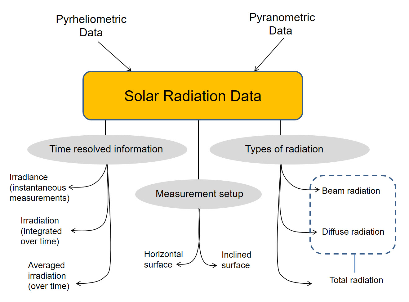
Solar radiation data collected through the above-mentioned instrumental methods provide the basis for development of any solar projects. We can summarize the types of solar resource data as follows:

Figure 2.2. Overview of different types of solar radiation data.

Click here for a text description

Solar radiation data supplied via pyrheliometric and pyranometric measurements may represent time resolved information: e.g., irradiance (instantaneous measurements of solar energy flux), irradiation (integrated energy flux over time), or averaged irradiation. Depending on measurement setup, the data can be for horizontal or inclined surface. The data can characterize different types of radiation: beam, diffuse, or total.

Credit: Mark Fedkin

Before moving on, please work through the following self-check questions to assess your learning:

2.2 Types and Elements of Concentrating Collectors

Any general setup for the conversion of the solar energy includes a receiver - a device that is able to convert the solar radiation into a different kind of energy. This can be either a heat absorber (to harvest thermal energy) or a photovoltaic cell (to convert light to electric energy). In the first case, the thermal radiation is absorbed to heat a medium (fluid), which transfers that absorbed energy to a generator. In the second case, light causes a photovoltaic effect in the material of the solar cell, which generates electric current. In both of these situations, the amount of energy available for the conversion is only as much as the solar source supplies per unit area of the converter.

If we need more energy for use, we have two options. The first option is to increase the system scale (for example by increasing the number of receivers). In other words, we have to expand the plant area, which would involve additional cost for construction, service, maintenance, and may require additional land, more materials, etc. It has been done to some extent, but sometimes it is not a sufficient measure to meet the energy demands, especially if land area is a constraint. The second option is to concentrate the radiation flux. This can be achieved by placing a concentrator (usually some kind of optical device) between the light source (sun) and the receiver. By common terminology, a solar collector is a sunlight processing system that includes a concentrator and a receiver in its setup; it is also characterized by aperture - the cross sectional area through which sunlight accesses the system.

The most common concentrators are reflectors (mirrors) and refractors (lenses), which modify and redirect the incident sunlight beam. The design of the concentrating optics varies. Some of the examples of concentrating collectors, which involve diversely shaped mirrors, are shown in Figure 2.3, as they applied to the solar-to-thermal energy conversion.

Figure 2.3. Types of concentrating sunlight collectors: (a) tubular absorbers with diffuse back reflector, (b) tubular absorbers with specular cusp reflectors, (c) plane receiver with plain reflectors (V-trough), (d) multisectional planar concentrator, (e) compound parabolic concentrator (f) parabolic trough, (g) fresnel concentrator, (h) array reflectors (heliostats) with central receiver. Concentration of light on the receiver is achieved by shaping the reflectors (mirrors) around the receiver (represented by blue circles).

Credit: Mark Fedkin - modified after Duffie and Beckman, 2013

The process of light concentration implies first of all that the energy flux is increased due to confining it to a smaller area. This brings several important benefits:

• reaching higher temperatures for heat collectors;
• heat losses from the surface of the receiver are decreased because the receiving area is decreased;
• higher energy conversion rate can be achieved over smaller area.

There are two major classes of solar concentrators: imaging and non-imaging. Imaging concentrators are called imaging because they produce an optical image of the sun on the receiver. Non-imaging concentrators do not produce such an image, but rather disperse the light from the sun over the whole area of the receiver. Non-imaging concentrators have relatively low concentration ratio (<10) compared to the imaging concentrators.

All of the optical tools designed for manipulating sunlight for the purpose of its concentration and efficient utilization are based on the fundamental optics principles, which you may remember from physics courses. In case you need to refresh your knowledge of those fundamentals before we study the light concentration principles, please refer to the following reading and video:

Out of the different types of concentrators listed above, mainly the following four technologies have been adopted for use in the utility scale CSP facilities [Mendelsohn et al., 2012]:

1. Parabolic trough
2. Solar tower
3. Parabolic dish
4. Linear Fresnel reflector

All of these are imaging concentrators which allow relatively high concentration temperatures: about 400 ^oC for parabolic troughs, up to 650 ^oC for Stirling dishes, and above 1000 ^oC for solar power towers. Just for comparison, non-imaging concentrators would work maximum up to 200 ^oC. These technologies will be introduced in more detail in Lessons 7 and 8 of this course.

There are also developments for non-imaging compound parabolic collectors (CPC) to be used at the utility scale for low-temperature applications [Baig et al., 2009], but this technology is not as widespread due to its moderate concentrating capabilities. Its flexibility with respect to using non-beam radiation and more relaxed technical requirements to positioning of concentrators are still attractive, so this technology will be also included in our consideration.

Concentrating photovoltaics is another technology class that uses concentrated light, but those devices will be covered separately in Lessons 5 and 6 of this course.

2.3 Concentration Ratio

The light concentration process is typically characterized by the concentration ratio (C). By physical meaning, the concentration ratio is the factor by which the incident energy flux (I_o) is optically enhanced on the receiving surface (I_r) - see Figure 2.4. So, confining the available energy coming through a chosen aperture to a smaller area on the receiver, we should be able to increase the flux.

In the above equation, C_geo is called the geometric concentration ratio. It is easy to use, as the areas of the devices are known, although it is adequate only when the radiation flux is uniform over the aperture and over the receiver. Also, please note that for some imaging concentrators, the area of the available receiver surface can be different from the area of the image produced by the concentrator on the receiver. So, if the image does not cover the entire surface of the receiver, we need to use the image area to estimate the concentration ratio.

Figure 2.4. Schematic representation of light concentration process.

Credit: Mark Fedkin

The concentration ratio can also be represented by the energy flux ratio at the aperture and at the receiver. In this case, it is termed optical concentration ratio C_opt (or flux concentration ratio) and can be directly applied to thermal calculations.

In case the ambient energy flux over the aperture (insolation) and over the receiver (irradiance) is uniform, the geometric and optical concentration ratios are equal (C_geo = C_opt).

The concentration ratios are important metrics used to characterize and rank optical concentrators. Next, we will look at several examples of concentrator designs and see what values of concentration ratios they can provide.

There is a theoretical limit to solar concentration. For circular concentrators - 45,000, and for linear concentrators - 212, based on the geometrical considerations; however, these limits may be unreachable by real systems because of non-idealities and losses. If you are interested in the analytical estimation of the concentration limits, refer to Duffie and Beckman's (2013) book (p.325) for more details.

In general sunlight, concentration systems are roughly classified into: low concentration range (C<10), medium concentration range (10<C<100), and high concentration range (C>100). However, only some of the systems provide uniform concentrated light flux (e.g., V-troughs or pyramidal plane reflectors) and can be characterized by a single concentration ratio. Many systems with curved reflecting surfaces (e.g., conical, parabolic, spherical) create a distribution of flux density over the receiver and would rather be characterized by a variable C over the receiver width. In that case, a local concentration ratio (C_l) is the main parameter to characterize the performance of the ideal concentrator:

where I(y) is determined for any local position y from the center of the produced image, and I_ap is the intensity of the incident radiation at the aperture.

Figure 2.5. Example of distribution of local radiation intensity over the receiver of an imaging collector.

Credit: Mark Fedkin after Duffie and Beckman, 2013

In many typical cases of imaging concentrators, the reflectance of the surface (ρ), i.e., the fraction of light radiation reflected from the surface compared to the total incident radiation, is also taken into account. Then the local intensity of the concentrated light, I(y), can be described as follows:

Further, in this lesson, we will study some examples that use this equation to estimate energy distribution within a concentrated image on the receiver. It would be better to have a specific type of concentrator to apply these concepts. Please read through the following text to enforce your understanding of the concentration ratios.

2.4 Concentration with a Parabolic Reflector

Parabolic geometry is the basis for such concentrating solar power (CSP) technologies as troughs or dishes. Parabolic trough is also considered one of the most mature and most commercially proven technologies in the utility scale CSP facilities (Mendelsohn et al., 2012), so we will look at the physical principles of parabolic concentrators in some more detail.

Geometrically, a parabola is a locus of points that lie on equal distance from a line (directrix) and a point (focus) - see Figure 2.6. For each point of the parabola, DR = FR. The distance VF between the vertex and focus of the parabola is the focal distance (f). The line perpendicular to the directrix that passes through the focus is the axis of the parabola; the axis divides the parabola into two parts that are symmetrical.

With origin at its vertex, and the axis of the parabola taken as x-axis, a parabola is described by the equation:

where f is the focal length.

Figure 2.6. Geometry of the parabola.

Credit: Mark Fedkin

By definition of the focal point of the parabola, all incoming rays parallel to the axis of the parabola are reflected through the focus. This provides an opportunity for light concentration by using parabolic surfaces. If we assume that solar light arrives to the surface as essentially parallel rays, and apply the Snell's law (the angle of reflection equals the angle of incidence), we can assign the focal point as an ideal location for the receiver (Figure 2.7).

Figure 2.7. Geometry of a parabolic reflector. All rays parallel to the parabola axis are reflected through the focal point.

Credit: Mark Fedkin

Solar applications deal with a parabola of a finite height (Figure 2.8). The design of the parabolic reflector takes into account the available aperture size (a), focus location (f - i.e., where receiver would be placed), and height of the reflector (h). These parameters are interrelated via the equation (Stine and Harrigan, 1986):

Figure 2.8. Corresponding variation of the parabolic curvature and focal distance for a fixed aperture.

Credit: Mark Fedkin

This figure above shows that the flatter the reflecting surface, the longer the focal length. The "flatness" of the shape of a finite parabola is typically characterized by the rim angle ($\varphi$ ). When rim angle increases (within the same aperture), the parabola becomes more curved, and the focal distance shortens.

Figure 2.9. Parabolic trough mirror installation on a solar farm.

Credit: Kuraymat (via Flickr) [8]

Parabolic trough (Figure 2.9) is a typical example of an imaging concentrator that utilizes the geometric relationships discussed above. Parabolic trough is one of the most widely implemented technologies for sunlight concentration at the utility scale. This type of collectors relies on sun tracking to ensure that the beam radiation is directed parallel to the parabolic axis.

A parabolic mirror produces an image of the sun on the surface of the receiver, so the receiver size needs to be matched to the image size. Consider Figure 2.10, which illustrates this idea. Since the sun is not really a point source, solar beam incident on the reflector is represented as a cone with an angular width 0.53^o (so the half-angle between the cone axis and its side is 0.267^o). Being reflected at a point on the parabolic surface, the beam hits the focal plane, where it produces an image of a certain dimension, centered around the focal point. The diameter of the cylindrical receiver (D), which would intercept the entire reflected image can be theoretically calculated using aperture width (a), and rim angle ($\varphi$ ) as follows (Duffie and Beckman, 2013):

Figure 2.10. Beam reflection in an imaging parabolic concentrator with aperture a. Blue area imitates the position of a cylindrical (tubular) receiver at the focal point. Gray area imitates a flat receiver at the focal plane. The minimal size of the receiver to intercept all of the reflected radiation should be matched to the diameter of the reflected beam at the focal plane.

Credit: Mark Fedkin - modified after Duffie and Beckman, 2013

For the linear receiver, the width of the image (W) produced on the focal plane can be determined as follows:

The equations presented here can be used to estimate the size of the reflected light image on the receiver for different shapes of parabolic reflectors. The formulas include a as a chosen aperture of the reflector (width of the trough), and ($\varphi$ ) as a measure of parabolic curvature. Note that these are the minimal theoretical dimensions of the reflected image that would be produced by the ideal parabolic mirror that is perfectly aligned. If there are any flaws in the mirror surface or trueness of the angle, additional spreading of the image may occur. If you are interested in more explanation of how these formulas were derived, please refer to Duffie and Beckman, 2013 book (Section 7.9)

The above-described geometrical concepts apply to the cross-section of a parabolic reflector. In reality, the reflector itself is a three-dimensional shape, i.e., a parabolic cylinder with a finite length (l). So, the cone-shaped ray reflected at a point on the surface of a parabolic reflector will produce an ellipse-shaped image on the focal plane. We can see that as the reflection point is moved away from the vertex towards the rim, the ellipse transforms from a circular to a more and more elongated shape (because the cone would be sectioned by the focal plane at greater and greater angle - Figure 2.11).

Figure 2.11. Cross section of a cone (shown as gray shaded area) in the direction perpendicular to its axis (left) and at an angle to its axis (right).

Credit: Mark Fedkin

Knowing the angular width of the cone, the dimensions of the ellipse image can be theoretically derived and presented as a function of $\varphi$ (angle of deviation from the parabola axis). Below are the equations describing the length of the minor and major axes of the ellipse.

where r is the distance between the focus and reflection point (local radius) on the parabolic mirror (r=f at the vertex); $\varphi$ is the angle between the parabola axis and the ray, and 0.267^o is the half-angle of the ray cone width.

The superposition of these individual ellipses produced by each element of the reflector form the total image, which is not uniform, but rather has a distribution of light intensity. The focal length (which is related to the rim angle of the reflector) is responsible for image size, while the aperture is responsible for the total amount of energy concentrated by a collector. So, the total image intensity (brightness) at the receiver should be a function of a/f. The image brightness essentially reflects the energy flux concentration:

The distribution of intensity of the energy flux within the concentrated image may have a profile similar to Figure 2.5. Different models have been applied to quantify that profile. For example, one of the approaches is called nonuniform solar disk, which suggests that the sunlight intensity coming out of the center of the solar disk is higher than that coming from its edges [Evans, 1977]. Without going into too much detail of this model, we can use the diagrams presented in the book by Duffie and Beckman (2013), which allow connecting various parameters of a parabolic concentrator with the local intensity on the receiver.

Please refer to the following reading to study the tools for image analysis via the nonuniform solar disk model, and be sure to study the example presented therein, which is very helpful.

Please answer the following quick questions to check your understanding of some of the basic points in this section. The parabola cheatsheet [9]presents a useful summary for your notes. 

2.5 CPC Collectors - Concentration of Diffuse Radiation

The compound parabolic concentrators (CPC) are typical representatives of non-imaging concentrators, which are capable of collecting all available radiation - both beam and diffuse - and directing it to the receiver. These concentrators do not have such strict requirements for the incidence angle as the parabolic troughs have, which makes them attractive from the point of view of system simplicity and flexibility. Like parabolic and other shapes, CPC concentrators can be applied in both linear (troughs) and three-dimensional (parabolocylinder) versions. The same as in "pure" parabola case, troughs are most widespread and useful for this type of concentrator.

The geometry of a CPC collector is demonstrated in Figure 2.12. If we consider a CPC trough, this diagram represents its cross-section. Each side of the shape is a parabola, and each of the parabolas has its focus at the lower edge of the other parabola (e.g., F is the focus of the right-hand parabola in Figure 2.12). Each parabola axis is tilted relative to the axis of the CPC shape. One of its key parameters is acceptance half-angle (${\theta }_c$), which is the angle between the axis of the collector and the line connecting the focus of one of the parabolas with the opposite edge of the aperture. The collector is designed in such a way that each ray coming into the CPC aperture at an angle smaller that $\theta$ reaches the receiver; if this angle is greater than ${\theta }_c$ , the ray will return (Figure 2.13). The relationship between the size of the aperture (2a), the size of the receiver (2a') and the acceptance half-angle is expressed through the following equation:

Knowing that the geometric concentration ratio is the quotient of the aperture area to the receiver area (see Section 2.3), for a linear CPC concentrator, we can obtain the relationship between the concentration ratio and the acceptance angle:

Figure 2.12. Geometry of the compound parabolic concentrator (CPC).

Click for a text description of the image

One large parabolic mirror with a second mirror sitting tangent to the parabolic axis with an end at mirror #1’s focus. The distance between the two upper ends of the parabolas is labeled aperture (2a) and the bottom two ends is labeled receiver. Dashed lines connect one top end to the opposite bottom end. The angle between their y intercept, y-axis and upper tip represents the acceptance half-angle.

Credit: Mark Fedkin after Duffie and Beckman, 2013

Figure 2.13. Reflection of light directed to the CPC concentrator at different angles. All rays with the angle of incidence smaller or equal to the acceptance angle reach the receiver at the bottom; all rays with the angle of incidence higher than the acceptance angle are reflected back to the aperture.

Credit: Mark Fedkin

There are some other useful expressions that describe the design of CPC concentrators. The following equations relate the focal distance of the side parabola (f) to the acceptance angle, receiver size, and height of the collector (Duffie and Beckman, 2013):

Please complete the following reading to further explore the work principle of CPC concentrators.

The following self-check questions will help you to test check your learning of the principles of CPC collectors:

Summary and Activities

Lesson 2 covers fundamental principles of light concentration that are important for a number of solar energy conversion technologies - both thermal and photovoltaic conversion. The general scheme of the solar energy concentration is this:

Input solar energy flux ⇒ Optical concentration device ⇒ Output concentrated solar energy flux

We touched upon each of these stages. First, we looked at the available solar radiation at the earth surface - the input we start with. Then, we considered a few techniques that concentrate the available flux, confining it to a smaller area. Finally, we looked at the output and its characteristics. Theoretical and empirical laws presented in the readings provide you with the background for estimating such parameters as concentration ratio and output energy density. Most of the theoretical considerations presented here are made for ideal systems. In reality, you can expect that imperfect optics will require additional corrections for non-ideality and losses. Limitations and advantages of specific concentrating technologies will be considered in further lessons, separately for CSP and photovoltaic systems.

After you have covered the assigned materials for this lesson, please complete the following assignments:

References for Lesson 2