Hidden Content Book
OLD Chapter 5: How We Know Where We Are: Land Surveying, GPS, and Technology
1. Overview
As you recall from Chapter 1, geographic data represent spatial locations and non-spatial attributes measured at certain times. We defined "feature" as a set of positions that specifies the location and extent of an entity. Positions, then, are a fundamental element of geographic data. Like the letters that make up these words, positions are the building blocks from which features are constructed. A property boundary, for example, is made up of a set of positions connected by line segments.
In theory, a single position is a "0-dimensional" feature: an infinitesimally small point from which 1-dimensional, 2-dimensional, and 3-dimensional features (lines, areas, and volumes) are formed. In practice, positions occupy 2- or 3-dimensional areas as a result of the limited resolution of measurement technologies and the limited precision of location coordinates. Resolution and precision are two aspects of data quality. This chapter explores the technologies and procedures used to produce positional data, and the factors that determine its quality.
Objectives
Students who successfully complete Chapter 5 should be able to:
- Identify and define the key aspects of data quality, including resolution, precision, and accuracy;
- List and explain the procedures land surveyors use to produce positional data, including traversing, triangulation, and trilateration;
- Calculate plane coordinates by open traverse;
- Calculate elevations by leveling;
- Explain how radio signals broadcast by Global Positioning System satellites are used to calculate positions on the surface of the Earth;
- State the kinds and magnitude of error associated with uncorrected GPS positioning; and
- Identify and explain methods used to improve the accuracy of GPS positioning.
Comments and Questions
Registered students are welcome to post comments, questions, and replies to questions about the text. Particularly welcome are anecdotes that relate the chapter text to your personal or professional experience. In addition, there are discussion forums available in the ANGEL course management system for comments and questions about topics that you may not wish to share with the whole world.
To post a comment, scroll down to the text box under "Post new comment" and begin typing in the text box, or you can choose to reply to an existing thread. When you are finished typing, click on either the "Preview" or "Save" button (Save will actually submit your comment). Once your comment is posted, you will be able to edit or delete it as needed. In addition, you will be able to reply to other posts at any time.
Note: the first few words of each comment become its "title" in the thread.
 |
Students who register for this Penn State course gain access to assignments and instructor feedback, and earn academic credit. Information about Penn State's Online Geospatial Education programs is available at http://gis.e-education.psu.edu [1]. |
2. Checklist
The following checklist is for Penn State students who are registered for classes in which this text, and associated quizzes and projects in the ANGEL course management system, have been assigned. You may find it useful to print this page out first so that you can follow along with the directions.
Chapter 5 Checklist (for registered students only) |
||
| Step | Activity | Access/Directions |
|---|---|---|
| 1 | Read Chapter 5 | This is the second page of the Chapter. Click on the links at the bottom of the page to continue or to return to the previous page, or to go to the top of the chapter. You can also navigate the text via the links in the GEOG 482 menu on the left. |
| 2 | Submit five practice quizzes including:
|
Go to ANGEL > [your course section] > Lessons tab > Chapter 5 folder > [quiz] |
| 3 | Perform "Try this" activities including:
"Try this" activities are not graded. |
Instructions are provided for each activity. |
| 4 | Submit the Chapter 5 Graded Quiz | ANGEL > [your course section] > Lessons tab > Chapter 5 folder > Chapter 5 Graded Quiz. See the Calendar tab in ANGEL for due dates. |
| 5 | Read comments and questions posted by fellow students. Add comments and questions of your own, if any. | Comments and questions may be posted on any page of the text, or in a Chapter-specific discussion forum in ANGEL. |
3. Geospatial Data Quality
Quality is a characteristic of comparable things that allows us to decide that one thing is better than another. In the context of geographic data, the ultimate standard of quality is the degree to which a data set is fit for use in a particular application. That standard is called validity. The standard varies from one application to another. In general, however, the key criteria are how much error is present in a data set, and how much error is acceptable.
Some degree of error is always present in all three components of geographic data: features, attributes, and time. Perfect data would fully describe the location, extent, and characteristics of phenomena exactly as they occur at every moment. Like the proverbial 1:1 scale map, however, perfect data would be too large, and too detailed to be of any practical use. Not to mention impossibly expensive to create in the first place!
4. Error and Uncertainty
Positions are the products of measurements. All measurements contain some degree of error. Errors are introduced in the original act of measuring locations on the Earth surface. Errors are also introduced when second- and third-generation data is produced, say, by scanning or digitizing a paper map.
In general, there are three sources of error in measurement: human beings, the environment in which they work, and the measurement instruments they use.
Human errors include mistakes, such as reading an instrument incorrectly, and judgments. Judgment becomes a factor when the phenomenon that is being measured is not directly observable (like an aquifer), or has ambiguous boundaries (like a soil unit).
Environmental characteristics, such as variations in temperature, gravity, and magnetic declination, also result in measurement errors.
Instrument errors follow from the fact that space is continuous. There is no limit to how precisely a position can be specified. Measurements, however, can be only so precise. No matter what instrument, there is always a limit to how small a difference is detectable. That limit is called resolution.
The diagram below shows the same position (the point in the center of the bullseye) measured by two instruments. The two grid patterns represent the smallest objects that can be detected by the instruments. The pattern at left represents a higher-resolution instrument.
Resolution.
The resolution of an instrument affects the precision of measurements taken with it. In the illustration below, the measurement at left, which was taken with the higher-resolution instrument, is more precise than the measurement at right. In digital form, the more precise measurement would be represented with additional decimal places. For example, a position specified with the UTM coordinates 500,000 meters East and 5,000,000 meters North is actually an area 1 meter square. A more precise specification would be 500,000.001 meters East and 5,000,000.001 meters North, which locates the position within an area 1 millimeter square. You can think of the area as a zone of uncertainty within which, somewhere, the theoretically infinitesimal point location exists. Uncertainty is inherent in geospatial data.
The precision of a single measurement.
Precision takes on a slightly different meaning when it is used to refer to a number of repeated measurements. In the illustration below, there is less variance among the nine measurements at left than there is among the nine measurements at right. The set of measurements at left is said to be more precise.
The precision of multiple measurements.
Hopefully you have noticed that resolution and precision are independent from accuracy. As shown below, accuracy simply means how closely a measurement corresponds to an actual value.
Accuracy.
I mentioned the U.S. Geological Survey's National Map Accuracy Standard in Chapter 2. In regard to topographic maps, the Standard warrants that 90 percent of well-defined points tested will be within a certain tolerance of their actual positions. Another way to specify the accuracy of an entire spatial database is to calculate the average difference between many measured positions and actual positions. The statistic is called the root mean square error (RMSE) of a data set.
5. Systematic vs. Random Errors
The diagram below illustrates the distinction between systematic and random errors. Systematic errors tend to be consistent in magnitude and/or direction. If the magnitude and direction of the error is known, accuracy can be improved by additive or proportional corrections. Additive correction involves adding or subtracting a constant adjustment factor to each measurement; proportional correction involves multiplying the measurement(s) by a constant.
Unlike systematic errors, random errors vary in magnitude and direction. It is possible to calculate the average of a set of measured positions, however, and that average is likely to be more accurate than most of the measurements.
Systematic and random errors.
In the sections that follow we compare the accuracy and sources of error of two important positioning technologies: land surveying and the Global Positioning System.
6. Survey Control
Geographic positions are specified relative to a fixed reference. Positions on the globe, for instance, may be specified in terms of angles relative to the center of the Earth, the equator, and the prime meridian. Positions in plane coordinate grids are specified as distances from the origin of the coordinate system. Elevations are expressed as distances above or below a vertical datum such as mean sea level, or an ellipsoid such as GRS 80 or WGS 84, or a geoid.
Land surveyors measure horizontal positions in geographic or plane coordinate systems relative to previously surveyed positions called control points. In the U.S., the National Geodetic Survey (NGS) maintains a National Spatial Reference System (NSRS) that consists of approximately 300,000 horizontal and 600,000 vertical control stations (Doyle,1994). Coordinates associated with horizontal control points are referenced to NAD 83; elevations are relative to NAVD 88. In a Chapter 2 activity you may have retrieved one of the datasheets that NGS maintains for every NSRS control point, along with more than a million other points submitted by professional surveyors.

Benchmark used to mark a vertical control point. (Thompson, 1988).
In 1988 NGS established four orders of control point accuracy, which are outlined in the table below. The minimum accuracy for each order is expressed in relation to the horizontal distance separating two control points of the same order. For example, if you start at a control point of order AA and measure a 500 km distance, the length of the line should be accurate to within 3 mm base error, plus or minus 5 mm line length error (500,000,000 mm × 0.01 parts per million).
| Order | Survey activities |
Maximum base error (95% confidence limit) |
Maximum Line-length dependent error (95% confidence limit) |
| AA | Global-regional dynamics; deformation measurements | 3 mm |
1:100,000,000
(0.01 ppm)
|
| A | NSRS primary networks | 5 mm | 1:10,000,000 (0.1 ppm) |
| B | NSRS secondary networks; high-precision engineering surveys | 8 mm | 1:1,000,000 (1 ppm) |
| C | NSRS terrestrial; dependent control surveys for mapping, land information, property, and engineering requirements | 1st: 1.0 cm 2nd-I: 2.0 cm 2nd-II: 3.0 cm 3rd: 5.0 cm |
1st: 1:100,000 2nd-I: 1:50,000 2nd-II: 1:20,000 3rd: 1:10,000 |
Control network accuracy standards used for U.S. National Spatial Reference System (Federal Geodetic Control Committee, 1988).
Doyle (1994) points out that horizontal and vertical reference systems coincide by less than ten percent. This is because
....horizontal stations were often located on high mountains or hilltops to decrease the need to construct observation towers usually required to provide line-of-sight for triangulation, traverse and trilateration measurements. Vertical control points however, were established by the technique of spirit leveling which is more suited to being conducted along gradual slopes such as roads and railways that seldom scale mountain tops. (Doyle, 2002, p. 1)
You might wonder how a control network gets started. If positions are measured relative to other positions, what is the first position measured relative to? The answer is: the stars. Before reliable timepieces were available, astronomers were able to determine longitude only by careful observation of recurring celestial events, such as eclipses of the moons of Jupiter. Nowadays geodesists produce extremely precise positional data by analyzing radio waves emitted by distant stars. Once a control network is established, however, surveyors produce positions using instruments that measure angles and distances between locations on the Earth's surface.
7. Measuring Angles
Angles can be measured with a magnetic compass, of course. Unfortunately, the Earth's magnetic field does not yield the most reliable measurements. The magnetic poles are not aligned with the planet's axis of rotation (an effect called magnetic declination), and they tend to change location over time. Local magnetic anomalies caused by magnetized rocks in the Earth's crust and other geomagnetic fields make matters worse.
For these reasons land surveyors rely on transits (or their more modern equivalents, called theodolites) to measure angles. A transit consists of a telescope for siting distant target objects, two measurement wheels that work like protractors for reading horizontal and vertical angles, and bubble levels to ensure that the angles are true. A theodolite is essentially the same instrument, except that some mechanical parts are replaced with electronics.

Transit. (Raisz, 1948). Used by permission.
Surveyors express angles in several ways. When specifying directions, as is done in the preparation of a property survey, angles may be specified as bearings or azimuths. A bearing is an angle less than 90° within a quadrant defined by the cardinal directions. An azimuth is an angle between 0° and 360° measured clockwise from North. "South 45° East" and "135°" are the same direction expressed as a bearing and as an azimuth. An interior angle, by contrast, is an angle measured between two lines of sight, or between two legs of a traverse (described later in this chapter).

Azimuths and bearings.
In the U.S., professional organizations like the American Congress on Surveying and Mapping, the American Land Title Association, the National Society of Professional Surveyors, and others, recommend minimum accuracy standards for angle and distance measurements. For example, as Steve Henderson (personal communication, Fall 2000, updated July 2010) points out, the Alabama Society of Professional Land Surveyors (http://www.aspls.org/Standards_of_Practice.html [2]) recommends that errors in angle measurements in "commercial/high risk" surveys be no greater than 15 seconds times the square root of the number of angles measured.
To achieve this level of accuracy, surveyors must overcome errors caused by faulty instrument calibration; wind, temperature, and soft ground; and human errors, including misplacing the instrument and misreading the measurement wheels. In practice, surveyors produce accurate data by taking repeated measurements and averaging the results.
8. Measuring Distances
To measure distances, land surveyors once used 100-foot long metal tapes that are graduated in hundredths of a foot. (This is the technique I learned as a student in a surveying class at the University of Wisconsin in the early 1980s. The picture shown below is slightly earlier.) Distances along slopes are measured in short horizontal segments. Skilled surveyors can achieve accuracies of up to one part in 10,000 (1 centimeter error for every 100 meters distance). Sources of error include flaws in the tape itself, such as kinks; variations in tape length due to extremes in temperature; and human errors such as inconsistent pull, allowing the tape to stray from the horizontal plane, and incorrect readings.
Surveying team measuring a baseline distance with a metal (Invar) tape. (Hodgson, 1916).
Since the 1980s, electronic distance measurement (EDM) devices have allowed surveyors to measure distances more accurately and more efficiently than they can with tapes. To measure the horizontal distance between two points, one surveyor uses an EDM instrument to shoot an energy wave toward a reflector held by the second surveyor. The EDM records the elapsed time between the wave's emission and its return from the reflector. It then calculates distance as a function of the elapsed time. Typical short-range EDMs can be used to measure distances as great as 5 kilometers at accuracies up to one part in 20,000, twice as accurate as taping.
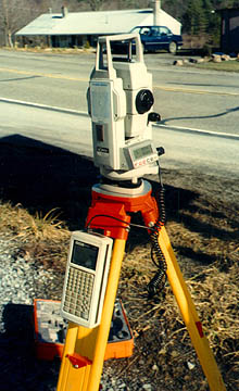
Total station.
Instruments called total stations combine electronic distance measurement and the angle measuring capabilities of theodolites in one unit. Next we consider how these instruments are used to measure horizontal positions in relation to established control networks.
9. Horizontal Positions
Surveyors have developed distinct methods, based on separate control networks, for measuring horizontal and vertical positions. In this context, a horizontal position is the location of a point relative to two axes: the equator and the prime meridian on the globe, or x and y axes in a plane coordinate system. Control points tie coordinate systems to actual locations on the ground; they are the physical manifestations of horizontal datums. In the following pages we review two techniques that surveyors use to create and extend control networks (triangulation and trilateration) and two other techniques used to measure positions relative to control points (open and closed traverses).
10. Traverse
Surveyors typically measure positions in series. Starting at control points, they measure angles and distances to new locations, and use trigonometry to calculate positions in a plane coordinate system. Measuring a series of positions in this way is known as "running a traverse." A traverse that begins and ends at different locations is called an open traverse.
An open traverse. (Adapted from Robinson, et al., 1995)
For example, say the UTM coordinates of point A in the illustration above are 500,000.00 E and 5,000,000.00 N. The distance between points A and P, measured with a steel tape or an EDM, is 2,828.40 meters. The azimuth of the line AP, measured with a transit or theodolite, is 45º. Using these two measurements, the UTM coordinates of point P can be calculated as follows:
XP = 500,000.00 + (2,828.40 × sin 45) = 501,999.98
YP = 5,000,000.00 + (2,828.40 × cos 45°) = 5,001,999.98
A traverse that begins and ends at the same point, or at two different but known points, is called a closed traverse. Measurement errors in a closed traverse can be quantified by summing the interior angles of the polygon formed by the traverse. The accuracy of a single angle measurement cannot be known, but since the sum of the interior angles of a polygon is always (n-2) × 180, it's possible to evaluate the traverse as a whole, and to distribute the accumulated errors among all the interior angles.
Errors produced in an open traverse, one that does not end where it started, cannot be assessed or corrected. The only way to assess the accuracy of an open traverse is to measure distances and angles repeatedly, forward and backward, and to average the results of calculations. Because repeated measurements are costly, other surveying techniques that enable surveyors to calculate and account for measurement error are preferred over open traverses for most applications.
11. Triangulation
Closed traverses yield adequate accuracy for property boundary surveys, provided that an established control point is nearby. Surveyors conduct control surveys to extend and densify horizontal control networks. Before survey-grade satellite positioning was available, the most common technique for conducting control surveys was triangulation.
The purpose of a control survey is to establish new horizontal control points (B, C, and D) based upon an existing control point (A).
Using a total station equipped with an electronic distance measurement device, the control survey team commences by measuring the azimuth alpha, and the baseline distance AB. These two measurements enable the survey team to calculate position B as in an open traverse. Before geodetic-grade GPS became available, the accuracy of the calculated position B may have been evaluated by astronomical observation.
Establishing a second control point (B) in a triangulation network.
The surveyors next measure the interior angles CAB, ABC, and BCA at point A, B, and C. Knowing the interior angles and the baseline length, the trigonometric "law of sines" can then be used to calculate the lengths of any other side. Knowing these dimensions, surveyors can fix the position of point C.
Establishing the position of point C by triangulation.
Having measured three interior angles and the length of one side of triangle ABC, the control survey team can calculate the length of side BC. This calculated length then serves as a baseline for triangle BDC. Triangulation is thus used to extend control networks, point by point and triangle by triangle.
Extending the triangulation network.
13. Vertical Positions
A vertical position is the height of a point relative to some reference surface, such as mean sea level, a geoid, or an ellipsoid. The roughly 600,000 vertical control points in the U.S. National Spatial Reference System (NSRS) are referenced to the North American Vertical Datum of 1988 (NAVD 88). Surveyors created the National Geodetic Vertical Datum of 1929 (NGVD 29, the predecessor to NAVD 88), by calculating the average height of the sea at all stages of the tide at 26 tidal stations over 19 years. Then they extended the control network inland using a surveying technique called leveling. Leveling is still a cost-effective way to produce elevation data with sub-meter accuracy.
A leveling crew at work in 1916. (Hodgson, 1916).
The illustration above shows a leveling crew at work. The fellow under the umbrella is peering through the telescope of a leveling instrument. Before taking any measurements, the surveyor made sure that the telescope was positioned midway between a known elevation point and the target point. Once the instrument was properly leveled, he focused the telescope crosshairs on a height marking on the rod held by the fellow on the right side of the picture. The chap down on one knee is noting in a field book the height measurement called out by the telescope operator.
A level used for determining elevations.
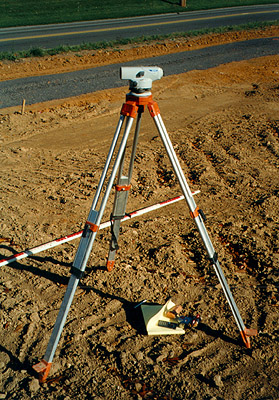
Leveling is still a cost-effective way to produce elevation data with sub-meter accuracy. A modern leveling instrument is shown in the photograph above. The diagram below illustrates the technique called differential leveling.

Differential leveling. (Adapted from Wolf & Brinker, 1994)
The diagram above illustrates differential leveling. A leveling instrument is positioned midway between a point at which the ground elevation is known (point A) and a point whose elevation is to be measured (B). The height of the instrument above the datum elevation is HI. The surveyor first reads a backsight measurement (BS) off of a leveling rod held by his trusty assistant over the benchmark at A. The height of the instrument can be calculated as the sum of the known elevation at the benchmark (ZA) and the backsight height (BS). The assistant then moves the rod to point B. The surveyor rotates the telescope 180°, then reads a foresight (FS) off the rod at B. The elevation at B (ZB) can then be calculated as the difference between the height of the instrument (HI) and the foresight height (FS).
Former student Henry Whitbeck (personal communication, Fall 2000) points out that surveyors also use total stations to measure vertical angles and distances between fixed points (prisms mounted upon tripods at fixed heights), then calculate elevations by trigonometric leveling.
Heights
Surveyors use the term height as a synonym for elevation. There are several different ways to measure heights. A properly-oriented level defines a line parallel to the geoid surface at that point (Van Sickle, 2001). An elevation above the geoid is called an orthometric height. However, GPS receivers cannot produce orthometric heights directly. Instead, GPS produces heights relative to the WGS 84 ellipsoid. Elevations produced with GPS are therefore called ellipsoidal (or geodetic) heights.
| Practice Quiz | Registered Penn State students should return now to the Chapter 5 folder in ANGEL (via the Resources menu to the left) to take a self-assessment quiz about Vertical Positions. You may take practice quizzes as many times as you wish. They are not scored and do not affect your grade in any way. |
|
Students who register for this Penn State course gain access to assignments and instructor feedback, and earn academic credit. Information about Penn State's Online Geospatial Education programs is available at http://gis.e-education.psu.edu [1]. |
14. Global Positioning System
Positioning signals broadcast from three Global Positioning System satellites are received at a location on Earth. (U.S. Federal Aviation Administration, 2007b)
The Global Positioning System (GPS) employs trilateration to calculate the coordinates of positions at or near the Earth's surface. Trilateration refers to the trigonometric law by which the interior angles of a triangle can be determined if the lengths of all three triangle sides are known. GPS extends this principle to three dimensions.
A GPS receiver can fix its latitude and longitude by calculating its distance from three or more Earth-orbiting satellites, whose positions in space and time are known. If four or more satellites are within the receiver's "horizon," the receiver can also calculate its elevation, and even its velocity. The U.S. Department of Defense created the Global Positioning System as an aid to navigation. Since it was declared fully operational in 1994, GPS positioning has been used for everything from tracking delivery vehicles, to tracking the minute movements of the tectonic plates that make up the Earth's crust, to tracking the movements of human beings. In addition to the so-called user segment made up of the GPS receivers and people who use them to measure positions, the system consists of two other components: a space segment and a control segment. It took about $10 billion to build over 16 years.
Russia maintains a similar positioning satellite system called GLONASS (http://www.glonass-ianc.rsa.ru [3]). Member nations of the European Union are in the process of deploying a comparable system of their own, called Galileo (http://www.esa.int/esaNA/ [4]). The first experimental GIOVE-A satellite began transmitting Galileo signals in January 2006. The goal of the Galileo project is a constellation of 30 navigation satellites by 2020. If the engineers and politicians succeed in making Galileo, GLONASS, and the U.S. Global Positioning System interoperable, as currently seems likely, the result will be a Global Navigation Satellite System (GNSS) that provides more than twice the signal-in-space resource that is available with GPS alone. The Chinese began work on their own system, called Beidou, in 2000. At the end of 2011 they had ten satellites in orbit, serving just China, with the goal being a global system of 35 satellites by 2020.
In this section you will learn to:
- Explain how radio signals broadcast by Global Positioning System satellites are used to calculate positions on the surface of the Earth; and
- Describe the functions of the space, control, and user segments of the Global Positioning System.
15. Space Segment
The space segment of the Global Positioning System currently consists of approximately 30 active and spare NAVSTAR satellites (new satellites are launched periodically, and old ones are decommissioned). "NAVSTAR" stands for "NAVigation System with Timing And Ranging." Each satellite circles the Earth every 12 hours in sidereal time along one of six orbital "planes" at an altitude of 20,200 km (about 12,500 miles). The satellites broadcast signals used by GPS receivers on the ground to measure positions. The satellites are arrayed such that at least four are "in view" everywhere on or near the Earth's surface at all times, with typically up to eight and potentially 12 "in view" at any given time.

The constellation of GPS satellites. Illustration © Smithsonian Institution, 1988. Used by Permission.
| Try This! | The U.S. Coast Guard's Navigation Center publishes status reports on the GPS satellite constellation. Its report of August 17, 2010, for example, listed 31 satellites, five to six in each of the six orbits planes (A-F), and one scheduled outage, on August 19, 2010. You can look up the current status of the constellation at http://www.navcen.uscg.gov/index.php [5] |

Artist's rendition of a NAVSTAR satellite (NAVSTAR GPS Joint Program Office, n.d.).
| Try This! | Scientific programmers at the U.S. National Aeronautics and Space Administration (NASA) have created an interactive, three-dimensional model of the Earth and the orbits of the more than 500 man-made satellites that surround it. The model is a Java applet called J-Track 3D Satellite Tracking (http://science.nasa.gov/realtime/jtrack/3d/JTrack3D.html/ [6]). Your browser must have Java enabled to view the applet. Instructions at the site describe how you can zoom in and out, and drag to rotate the model. To view orbits of particular satellites, choose Select from the Satellite menu. The Block IIA and R series are the most current generation of NAVSTAR satellites. |
16. Control Segment
The control segment of the Global Positioning System is a network of ground stations that monitors the shape and velocity of the satellites' orbits. The accuracy of GPS data depends on knowing the positions of the satellites at all times. The orbits of the satellites are sometimes disturbed by the interplay of the gravitational forces of the Earth and Moon.

The control segment of the Global Positioning System (U.S. Federal Aviation Administration, 2007b).
Monitor Stations are very precise GPS receivers installed at known locations. They record discrepancies between known and calculated positions caused by slight variations in satellite orbits. Data describing the orbits are produced at the Master Control Station at Colorado Springs, uploaded to the satellites, and finally broadcast as part of the GPS positioning signal. GPS receivers use this satellite Navigation Message data to adjust the positions they measure.
If necessary, the Master Control Center can modify satellite orbits by commands transmitted via the control segment's ground antennas.
17. User Segment
The U.S. Federal Aviation Administration (FAA) estimated in 2006 that some 500,000 GPS receivers are in use for many applications, including surveying, transportation, precision farming, geophysics, and recreation, not to mention military navigation. This was before in-car GPS navigation gadgets emerged as one of the most popular consumer electronic gifts during the 2007 holiday season in North America.
Basic consumer-grade GPS receivers, like the rather old-fashioned one shown below, consist of a radio receiver and internal antenna, a digital clock, some sort of graphic and push-button user interface, a computer chip to perform calculations, memory to store waypoints, jacks to connect an external antenna or download data to a computer, and flashlight batteries for power. The radio receiver in the unit shown below includes 12 channels to receive signal from multiple satellites simultaneously.

Recreation-grade GPS receiver, circa 1998.
NAVSTAR Block II satellites broadcast at two frequencies, 1575.42 MHz (L1) and 1227.6 MHz (L2). (For sake of comparison, FM radio stations broadcast in the band of 88 to 108 MHz.) Only L1 was intended for civilian use. Single-frequency receivers produce horizontal coordinates at an accuracy of about three to seven meters (or about 10 to 20 feet) at a cost of about $100. Some units allow users to improve accuracy by filtering out errors identified by nearby stationary receivers, a post-process called "differential correction." $300-500 single-frequency units that can also receive corrected L1 signals from the U.S. Federal Aviation Administration's Wide Area Augmentation System (WAAS) network of ground stations and satellites can perform differential correction in "real-time." Differentially-corrected coordinates produced by single-frequency receivers can be as accurate as one to three meters (about 3 to 10 feet).
The signal broadcast at the L2 frequency is encrypted for military use only. Clever GPS receiver makers soon figured out, however, how to make dual-frequency models that can measure slight differences in arrival times of the two signals (these are called "carrier phase differential" receivers). Such differences can be used to exploit the L2 frequency to improve accuracy without decoding the encrypted military signal. Survey-grade carrier-phase receivers able to perform real-time kinematic (RTK) differential correction, can produce horizontal coordinates at sub-meter accuracy at a cost of $1000 to $2000. No wonder GPS has replaced electro-optical instruments for many land surveying tasks.
Meanwhile, a new generation of NAVSTAR satellites (the Block IIR-M series) will add a civilian signal at the L2 frequency that will enable substantially improved GPS positioning.
18. Satellite Ranging
GPS receivers calculate distances to satellites as a function of the amount of time it takes for satellites' signals to reach the ground. To make such a calculation, the receiver must be able to tell precisely when the signal was transmitted, and when it was received. The satellites are equipped with extremely accurate atomic clocks, so the timing of transmissions is always known. Receivers contain cheaper clocks, which tend to be sources of measurement error. The signals broadcast by satellites, called "pseudo-random codes," are accompanied by the broadcast ephemeris data that describes the shapes of satellite orbits.

GPS receivers calculate distance as a function of the difference in time of broadcast and reception of a GPS signal. (Adapted from Hurn, 1989).
The GPS constellation is configured so that a minimum of four satellites is always "in view" everywhere on Earth. If only one satellite signal was available to a receiver, the set of possible positions would include the entire range sphere surrounding the satellite.

Set of possible positions of a GPS receiver relative to a single GPS satellite. (Adapted from Hurn, 1993).
If two satellites are available, a receiver can tell that its position is somewhere along a circle formed by the intersection of two spherical ranges.

Set of possible positions of a GPS receiver relative to two GPS satellites. (Adapted from Hurn, 1993).
If distances from three satellites are known, the receiver's position must be one of two points at the intersection of three spherical ranges. GPS receivers are usually smart enough to choose the location nearest to the Earth's surface. At a minimum, three satellites are required for a two-dimensional (horizontal) fix. Four ranges are needed for a three-dimensional fix (horizontal and vertical).

Set of possible positions of a GPS receiver relative to three GPS satellites. (Adapted from Hurn, 1993).
Satellite ranging is similar in concept to the plane surveying method trilateration, by which horizontal positions are calculated as a function of distances from known locations. The GPS satellite constellation is in effect an orbiting control network.
| Try This! | Trimble has a tutorial "designed to give you a good basic understanding of the principles behind GPS without loading you down with too much technical detail". Check it out at http://www.trimble.com/gps/index.shtml [7]. Click "Why GPS?" to get started. |
| Practice Quiz | Registered Penn State students should return now to the Chapter 5 folder in ANGEL (via the Resources menu to the left) to take a self-assessment quiz about GPS Components. You may take practice quizzes as many times as you wish. They are not scored and do not affect your grade in any way. |
|
Students who register for this Penn State course gain access to assignments and instructor feedback, and earn academic credit. Information about Penn State's Online Geospatial Education programs is available at http://gis.e-education.psu.edu [1]. |
19. GPS Error Sources
A thought experiment (Wormley, 2004): Attach your GPS receiver to a tripod. Turn it on and record its position every ten minutes for 24 hours. Next day, plot the 144 coordinates your receiver calculated. What do you suppose the plot would look like?
Do you imagine a cloud of points scattered around the actual location? That's a reasonable expectation. Now, imagine drawing a circle or ellipse that encompasses about 95 percent of the points. What would the radius of that circle or ellipse be? (In other words, what is your receiver's positioning error?)
The answer depends in part on your receiver. If you used a hundred-dollar receiver, the radius of the circle you drew might be as much as ten meters to capture 95 percent of the points. If you used a WAAS-enabled, single frequency receiver that cost a few hundred dollars, your error ellipse might shrink to one to three meters or so. But if you had spent a few thousand dollars on a dual frequency, survey-grade receiver, your error circle radius might be as small as a centimeter or less. In general, GPS users get what they pay for.
As the market for GPS positioning grows, receivers are becoming cheaper. Still, there are lots of mapping applications for which it's not practical to use a survey-grade unit. For example, if your assignment was to GPS 1,000 manholes for your municipality, you probably wouldn't want to set up and calibrate a survey-grade receiver 1,000 times. How, then, can you minimize errors associated with mapping-grade receivers? A sensible start is to understand the sources of GPS error.
In this section you will learn to:
- State the kinds and magnitude of error and uncertainty associated with uncorrected GPS positioning; and
- Use a PDOP chart to determine the optimal times for GPS positioning at a given location and date.
Note: My primary source for the material in this section is Jan Van Sickle's text GPS for Land Surveyors, 2nd Ed. If you want a readable and much more detailed treatment of this material, I recommend Jan's book. See the bibliography at the end of this chapter for more information about this and other resources.
20. User Equivalent Range Errors
"UERE" is the umbrella term for all of the error sources below, which are presented in descending order of their contributions to the total error budget.
- Satellite clock: GPS receivers calculate their distances from satellites as a function of the difference in time between when a signal is transmitted by a satellite and when it is received on the ground. The atomic clocks on board NAVSTAR satellites are extremely accurate. They do tend to stray up to one millisecond of standard GPS time (which is calibrated to, but not identical to, to Coordinated Universal Time). The monitoring stations that make up the GPS "Control Segment" calculate the amount of clock drift associated with each satellite. GPS receivers that are able to make use of the clock correction data that accompanies GPS signals can reduce clock error significantly.
- Upper atmosphere (ionosphere): Space is nearly a vacuum, but the atmosphere isn't. GPS signals are delayed and deflected as they pass through the ionosphere, the outermost layers of the atmosphere that extend from approximately 50 to 1,000 km above the Earth's surface. Signals transmitted by satellites close to the horizon take a longer route through the ionosphere than signals from satellites overhead, and are thus subject to greater interference. The ionosphere's density varies by latitude, by season, and by time of day, in response to the Sun's ultraviolet radiation, solar storms and maximums, and the stratification of the ionosphere itself. The GPS Control Segment is able to model ionospheric biases, however. Monitoring stations transmit corrections to the NAVSTAR satellites, which then broadcast the corrections along with the GPS signal. Such corrections eliminate only about three-quarters of the bias, however, leaving the ionosphere the second largest contributor to the GPS error budget.
- Receiver clock: GPS receivers are equipped with quartz crystal clocks that are less stable than the atomic clocks used in NAVSTAR satellites. Receiver clock error can be eliminated, however, by comparing times of arrival of signals from two satellites (whose transmission times are known exactly).
- Satellite orbit: GPS receivers calculate coordinates relative to the known locations of satellites in space. Knowing where satellites are at any given moment involves knowing the shapes of their orbits as well as their velocities. The gravitational attractions of the Earth, Sun, and Moon all complicate the shapes of satellite orbits. The GPS Control Segment monitors satellite locations at all times, calculates orbit eccentricities, and compiles these deviations in documents called ephemerides. An ephemeris is compiled for each satellite and broadcast with the satellite signal. GPS receivers that are able to process ephemerides can compensate for some orbital errors.
- Lower atmosphere: (troposphere, tropopause, and stratosphere) The three lower layers of atmosphere encapsulate the Earth from surface to an altitude of about 50 km. The lower atmosphere delays GPS signals, adding slightly to the calculated distances between satellites and receivers. Signals from satellites close to the horizon are delayed the most, since they pass through more atmosphere than signals from satellites overhead.
- Multipath: Ideally, GPS signals travel from satellites through the atmosphere directly to GPS receivers. In reality, GPS receivers must discriminate between signals received directly from satellites and other signals that have been reflected from surrounding objects, such as buildings, trees, and even the ground. Some, but not all, reflected signals are identified automatically and rejected. Antennas are designed to minimize interference from signals reflected from below, but signals reflected from above are more difficult to eliminate. One technique for minimizing multipath errors is to track only those satellites that are at least 15° above the horizon, a threshold called the "mask angle."
Douglas Welsh (personal communication, Winter 2001), an Oil and Gas Inspector Supervisor with Pennsylvania's Department of Environmental Protection, wrote about the challenges associated with GPS positioning in our neck of the woods: "...in many parts of Pennsylvania the horizon is the limiting factor. In a city with tall buildings and the deep valleys of some parts of Pennsylvania it is hard to find a time of day when the constellation will have four satellites in view for any amount of time. In the forests with tall hardwoods, multipath is so prevalent that I would doubt the accuracy of any spot unless a reading was taken multiple times." Van Sickle (2005) points out, however, that GPS modernization efforts and the GNSS may well ameliorate such gaps.
Have you had similar experiences with GPS? If so, please post a comment to this page .
21. Dilution of Precision
The arrangement of satellites in the sky also affects the accuracy of GPS positioning. The ideal arrangement (of the minimum four satellites) is one satellite directly overhead, three others equally spaced near the horizon (above the mask angle). Imagine a vast umbrella that encompasses most of the sky, where the satellites form the tip and the ends of the umbrella spines.
GPS coordinates calculated when satellites are clustered close together in the sky suffer from dilution of precision (DOP), a factor that multiplies the uncertainty associated with User Equivalent Range Errors (UERE - errors associated with satellite and receiver clocks, the atmosphere, satellite orbits, and the environmental conditions that lead to multipath errors). The DOP associated with an ideal arrangement of the satellite constellation equals approximately 1, which does not magnify UERE. According to Van Sickle (2001), the lowest DOP encountered in practice is about 2, which doubles the uncertainty associated with UERE.
GPS receivers report several components of DOP, including Horizontal Dilution of Precision (HDOP) and Vertical Dilution of Precision (VDOP). The combination of these two components of the three-dimensional position is called PDOP - position dilution of precision. A key element of GPS mission planning is to identify the time of day when PDOP is minimized. Since satellite orbits are known, PDOP can be predicted for a given time and location. Various software products allow you to determine when conditions are best for GPS work.
MGIS student Jason Setzer (Winter 2006) offers the following illustrative anecdote:
I have had a chance to use GPS survey technology for gathering ground control data in my region and the biggest challenge is often the PDOP (position dilution of precision) issue. The problem in my mountainous area is the way the terrain really occludes the receiver from accessing enough satellite signals.
During one survey in Colorado Springs I encountered a pretty extreme example of this. Geographically, Colorado Springs is nestled right against the Rocky Mountain front ranges, with 14,000 foot Pike's Peak just west of the city. My GPS unit was easily able to 'see' five, six or even seven satellites while I was on the eastern half of the city. However, the further west I traveled, I began to see progressively less of the constellation, to the point where my receiver was only able to find one or two satellites. If a 180 degree horizon-to-horizon view of the sky is ideal, then in certain places I could see maybe 110 degrees.
There was no real work around, other than patience. I was able to adjust my survey points enough to maximize my view of the sky. From there it was just a matter of time... Each GPS bird has an orbit time of around twelve hours, so in a couple of instances I had to wait up to two hours at a particular location for enough of them to become visible. My GPS unit automatically calculates PDOP and displays the number of available satellites. So the PDOP value was never as low as I would have liked, but it did drop enough to finally be within acceptable limits. Next time I might send a vendor out for such a project!
| Try This! |
Trimble Inc., a leading manufacturer of GPS receivers, offers GPS mission planning software for free downloads. This activity will introduce you to the capabilities of the software, and will prepare you to answer questions about GPS mission planning later.
|
| Practice Quiz | Registered Penn State students should return now to the Chapter 5 folder in ANGEL (via the Resources menu to the left) to take a self-assessment quiz about GPS Error Sources. You may take practice quizzes as many times as you wish. They are not scored and do not affect your grade in any way. |
|
Students who register for this Penn State course gain access to assignments and instructor feedback, and earn academic credit. Information about Penn State's Online Geospatial Education programs is available at http://gis.e-education.psu.edu [1]. |
22. GPS Error Correction
A variety of factors, including the clocks in satellites and receivers, the atmosphere, satellite orbits, and reflective surfaces near the receiver, degrade the quality of GPS coordinates. The arrangement of satellites in the sky can make matters worse (a condition called dilution of precision). A variety of techniques have been developed to filter out positioning errors. Random errors can be partially overcome by simply averaging repeated fixes at the same location, although this is often not a very efficient solution. Systematic errors can be compensated for by modeling the phenomenon that causes the error and predicting the amount of offset. Some errors, like multipath errors caused when GPS signals are reflected from roads, buildings, and trees, vary in magnitude and direction from place to place. Other factors, including clocks, the atmosphere, and orbit eccentricities, tend to produce similar errors over large areas of the Earth's surface at the same time. Errors of this kind can be corrected using a collection of techniques called differential correction.
In this section you will learn to:
- Explain the concept of differential correction and other methods used to improve the accuracy of GPS positioning; and
- Perform differential correction using data and services of the U.S. National Geodetic Survey.
23. Differential Correction
Differential correction is a class of techniques for improving the accuracy of GPS positioning by comparing measurements taken by two or more receivers. Here's how it works:
The locations of two GPS receivers--one stationary, one mobile--are illustrated below. The stationary receiver (or "base station") continuously records its fixed position over a control point. The difference between the base station's actual location and its calculated location is a measure of the positioning error affecting that receiver at that location at each given moment. In this example, the base station is located about 25 kilometers from the mobile receiver (or "rover"). The operator of the mobile receiver moves from place to place. The operator might be recording addresses for an E-911 database, or trees damaged by gypsy moth infestations, or street lights maintained by a public works department

A GPS base station is fixed over a control point, while about 25 km away, a mobile GPS receiver is used to measure a series of positions.
The illustration below shows positions calculated at the same instant (3:01 pm) by the base station (left) and the mobile receiver (right).

Actual and calculated positions of a base station and mobile receiver.
The base station calculates the correction needed to eliminate the error in the position calculated at that moment from GPS signals. The correction is later applied to the position calculated by the mobile receiver at the same instant. The corrected position is not perfectly accurate because the kinds and magnitudes of errors affecting the two receivers are not identical, and because of the low frequency of the GPS timing code.

Error correction calculated at the base station is applied to the position calculated by the mobile receiver.

GPS base station used for differential correction. Notice that the antenna is located directly above a control point monument.
24. Real-Time Differential Correction
For differential correction to work, fixes recorded by the mobile receiver must be synchronized with fixes recorded by the base station (or stations). You can provide your own base station, or use correction signals produced from reference stations maintained by the U.S. Federal Aviation Administration, the U.S. Coast Guard, or other public agencies or private subscription services. Given the necessary equipment and available signals, synchronization can take place immediately ("real-time") or after the fact ("post-processing"). First let's consider real-time differential.
WAAS-enabled receivers are an inexpensive example of real-time differential correction. "WAAS" stands for Wide Area Augmentation System (http://gps.faa.gov [9]), a collection of about 25 base stations set up to improve GPS positioning at U.S. airport runways to the point that GPS can be used to help land airplanes (U.S. Federal Aviation Administration, 2007c). WAAS base stations transmit their measurements to a master station, where corrections are calculated and then uplinked to two geosynchronous satellites (19 are planned). The WAAS satellite then broadcasts differentially-corrected signals at the same frequency as GPS signals. WAAS signals compensate for positioning errors measured at WAAS base stations, as well as clock error corrections and regional estimates of upper-atmosphere errors (Yeazel, 2003). WAAS-enabled receivers devote one or two channels to WAAS signals, and are able to process the WAAS corrections. The WAAS network was designed to provide approximately 7-meter accuracy uniformly throughout its U.S. service area.
DGPS: The U.S. Coast Guard has developed a similar system, called the Differential Global Positioning Service (http://www.navcen.uscg.gov/?pageName=dgpsMain [10]). The DGPS network includes some 80 broadcast sites, each of which includes a survey-grade base station and a "radiobeacon" transmitter that broadcasts correction signals at 285-325 kHz (just below the AM radio band). DGPS-capable GPS receivers include a connection to a radio receiver that can tune in to one or more selected "beacons." Designed for navigation at sea near U.S. coasts, DGPS provides accuracies no worse than 10 meters. Stephanie Brown (personal communication, Fall 2003) reported that where she works in Georgia, "with a good satellite constellation overhead, [DGPS accuracy] is typically 4.5 to 8 feet."
Survey-grade real-time differential correction can be achieved using a technique called real-time kinematic (RTK) GPS. According to surveyor Laverne Hanley (personal communication, Fall 2000), "real-time kinematic requires a radio frequency link between a base station and the rover. I have achieved better than centimeter accuracy this way, although the instrumentation is touchy and requires great skill on the part of the operator. Several times I found that I had great GPS geometry, but had lost my link to the base station. The opposite has also happened, where I wanted to record positions and had a radio link back to the base station, but the GPS geometry was bad."
25. Post-Processed Differential Correction
Kinematic positioning can deliver accuracies of 1 part in 100,000 to 1 part in 750,000 with relatively brief observations of only one to two minutes each. For applications that require accuracies of 1 part in 1,000,000 or higher, including control surveys and measurements of movements of the Earth's tectonic plates, static positioning is required (Van Sickle, 2001). In static GPS positioning, two or more receivers measure their positions from fixed locations over periods of 30 minutes to two hours. The receivers may be positioned up to 300 km apart. Only dual frequency, carrier phase differential receivers capable of measuring the differences in time of arrival of the civilian GPS signal (L1) and the encrypted military signal (L2) are suitable for such high-accuracy static positioning.
CORS and OPUS: The U.S. National Geodetic Survey (NGS) maintains an Online Positioning User Service (OPUS) that enables surveyors to differentially-correct static GPS measurements acquired with a single dual frequency carrier phase differential receiver after they return from the field. Users upload measurements in a standard Receiver INdependent EXchange format (RINEX) to NGS computers, which perform differential corrections by referring to three selected base stations selected from a network of continuously operating reference stations. NGS oversees two CORS networks; one consisting of its 600 base stations of its own, another a cooperative of public and private agencies that agree to share their base station data and to maintain base stations to NGS specifications.

The Continuously Operating Reference Station network (CORS) (Snay, 2005)
The map above shows distribution of the combined national and cooperative CORS networks. Notice that station symbols are colored to denote the sampling rate at which base station data are stored. After 30 days, all stations are required to store base station data only in 30 second increments. This policy limits the utility of OPUS corrections to static positioning (although the accuracy of longer kinematic observations can also be improved). Mindful of the fact that the demand for static GPS is steadily declining, NGS' future plans include streaming CORS base station data for real-time use in kinematic positioning.
| Try This! |
This optional activity (contributed by Chris Piburn of CompassData Inc.) will guide you through the process of differentially-correcting static GPS measurements using the NGS' Online Positioning User Service (OPUS), which refers to the Continuously Operating Reference Station network (CORS). The context is a CompassData project that involved a carrier phase differential GPS survey in a remote study area in Alaska. The objective was to survey a set of nine ground control points (GCPs) that would later be used to orthorectify a client's satellite imagery. So remote is this area that no NGS control point was available at the time the project was carried out. The alternative was to establish a base station for the project and to fix its position precisely with reference to CORS stations in operation elsewhere in Alaska. The project team flew by helicopter to a hilltop located centrally within the study area. With some difficulty they hammered an 18 inch #5 rebar into the rocky soil to serve as a control monument. After setting up a GPS base station receiver over the rebar, they flew off to begin data collection with their rover receiver. Thanks to favorable weather, Chris and his team collected the nine required photo-identifiable GCPs on the first day. The centrally-located base station allowed the team to minimize distances between the base and the rover, which meant they could minimize the time required to fix each GCP. At the end of the day, the team had produced five hours of GPS data at the base station and nine fifteen-minute occupations at the GCPs As you might expect, the raw GPS data were not sufficiently accurate to meet project requirements. (The various sources of random and systematic errors that contribute to the uncertainty of GPS data are considered elsewhere in this chapter.) In particular, the monument hammered into the hilltop was unsuitable for use as a control point because the uncertainty associated with its position was too great. The project team's first step in removing positioning errors was to post-process the data using baseline processing software, which adjusts computed baseline distances (between the base station and the nine GCPs) by comparing the phase of the GPS carrier wave as it arrived simultaneously at both the base station and the rover. The next step was to fix the position of the base station precisely in relation to CORS stations operating elsewhere in Alaska. The following steps will guide you through the process of submitting the five hours of dual frequency base station data to the U.S. National Geodetic Survey's Online Positioning User Service (OPUS), and interpreting the results. (For information about OPUS, see http://www.ngs.noaa.gov/OPUS/about.html [11] ) 1. Download the GPS data file. The compressed RINEX format file is approximately 6 Mb in size and will take about 1 minute to download via high speed DSL or cable, or about 15 minutes via 56 Kbps modem. If you can't download this file, contact me right away so we can help you resolve the problem.
2. Examine the RINEX file.
The RINEX Observation file contains all the information about the signals that CompassData's base station receiver tracked during the Alaska survey. Explaining all the contents of the file is well beyond the scope of this activity. For now, note the lines that disclose the antenna type, approximate position of the antenna, and antenna height. You'll report these parameters to OPUS in the next step. 3. Submit GPS data to OPUS
When you receive your OPUS solution by return email, you will want to discover the magnitude of differential correction that OPUS calculated. To do this you'll need to determine (a) the uncorrected position originally calculated by the base station, (b) the corrected position calculated by OPUS, and (c) the mark-to-mark distance between the original and corrected positions. In addition to the original RINEX file you downloaded earlier, you'll need the OPUS solution and two free software utilities provided by NGS. Links to these utilities are listed below. 4. Determine the position of the base station receiver prior to differential correction.
5. Determine the corrected position of the base station receiver. The OPUS solution you receive by email reports corrected coordinates in Earth-Centered Earth-Fixed X, Y, Z, as geographic coordinates, and as UTM and State Plane coordinates. Look for the latitude and longitude coordinates and ellipsoidal height that are specified relative to the NAD 83 datum. They should be very close to:
6. Calculate the difference between the original and corrected base station positions. NGS provides another software utility to calculate the three-dimensional distance between two positions. Unlike the previous XYZ to GEODETIC converter, however, the "invers3d.exe" is a program you download to your computer.
|

| Practice Quiz | Registered Penn State students should return now to the Chapter 5 folder in ANGEL (via the Resources menu to the left) to take a self-assessment quiz about GPS Error Correction. You may take practice quizzes as many times as you wish. They are not scored and do not affect your grade in any way. |
|
Students who register for this Penn State course gain access to assignments and instructor feedback, and earn academic credit. Information about Penn State's Online Geospatial Education programs is available at http://gis.e-education.psu.edu [1]. |
26. Summary
Positions are a fundamental element of geographic data. Sets of positions form features, as the letters on this page form words. Positions are produced by acts of measurement, which are susceptible to human, environmental, and instrument errors. Measurement errors cannot be eliminated, but systematic errors can be estimated, and compensated for.
Land surveyors use specialized instruments to measure angles and distances, from which they calculate horizontal and vertical positions. The Global Positioning System (and to a potentially greater extent, the emerging Global Navigation Satellite System) enables both surveyors and ordinary citizens to determine positions by measuring distances to three or more Earth-orbiting satellites. As you've read in this chapter (and may known from personal experience), GPS technology now rivals electro-optical positioning devices (i.e., "total stations" that combine optical angle measurement and electronic distance measurement instruments) in both cost and performance. This raises the question, "If survey-grade GPS receivers can produce point data with sub-centimeter accuracy, why are electro-optical positioning devices still so widely used?" In November 2005 I posed this question to two experts--Jan Van Sickle and Bill Toothill--whose work I had used as references while preparing this chapter. I also enjoyed a fruitful discussion with an experienced student named Sean Haile (Fall 2005). Here's what they had to say:
Jan Van Sickle, author of GPS for Land Surveyors and Basic GIS Coordinates, wrote:
In general it may be said that the cost of a good total station (EDM and theodolite combination) is similar to the cost of a good 'survey grade' GPS receiver. While a new GPS receiver may cost a bit more, there are certainly deals to be had for good used receivers. However, in many cases a RTK system that could offer production similar to an EDM requires two GPS receivers and there, obviously, the cost equation does not stand up. In such a case the EDM is less expensive.
Still, that is not the whole story. In some circumstances, such as large topographic surveys, the production of RTK GPS beats the EDM regardless of the cost differential of the equipment. Remember, you need line of sight with the EDM. Of course, if a topo survey gets too large, it is more cost effective to do the work with photogrammetry. And if it gets really large, it is most cost effective to use satellite imagery and remote sensing technology.
Now, lets talk about accuracy. It is important to keep in mind that GPS is not able to provide orthometric heights (elevations) without a geoid model. Geoid models are improving all the time, but are far from perfect. The EDM on the other hand has no such difficulty. With proper procedures it should be able to provide orthometric heights with very good relative accuracy over a local area. But, it is important to remember that relative accuracy over a local area with line of sight being necessary for good production (EDM) is applicable to some circumstances, but not others. As the area grows larger, as line of sight is at a premium, and a more absolute accuracy is required the advantage of GPS increases.
It must also be mentioned that the idea that GPS can provide cm level accuracy must always be discussed in the context of the question, 'relative to what control and on what datum?'
In relative terms, over a local area, using good procedures, it is certainly possible to say that an EDM can produce results superior to GPS in orthometric heights (levels) with some consistency. It is my opinion that this idea is the reason that it is rare for a surveyor to do detailed construction staking with GPS, i.e. curb and gutter, sewer, water, etc. On the other hand, it is common for surveyors to stake out property corners with GPS on a development site, and other features where the vertical aspect is not critical. It is not that GPS cannot provide very accurate heights, it is just that it takes more time and effort to do so with that technology when compared with EDM in this particular area (vertical component).
It is certainly true that GPS is not well suited for all surveying applications. However, there is no surveying technology that is well suited for all surveying applications. On the other hand, it is my opinion that one would be hard pressed to make the case that any surveying technology is obsolete. In other words, each system has strengths and weaknesses and that applies to GPS as well.
Bill Toothill, professor in the Department of GeoEnvironmental Sciences and Engineering at Wilkes University, wrote:
GPS is just as accurate at short range and more accurate at longer distances than electro-optical equipment. The cost of GPS is dropping and may not be much more than a high end electro-optical instrument. GPS is well suited for all surveying applications, even though for a small parcel (less than an acre) traditional instruments like a total station may prove faster. This depends on the availability of local reference sites (control) and the coordinate system reference requirements of the survey.
Most survey grade GPS units (dual frequency) can achieve centimeter level accuracies with fairly short occupation times. In the case of RTK this can be as little as five seconds with proper communication to a broadcasting 'base'. Sub-centimeter accuracies is another story. To achieve sub-centimeter, which most surveyors don't need, requires much longer occupation times which is not conducive for 'production' work in a business environment. Most sub-centimeter applications are used for research, most of which are in the geologic deformation category. I have been using dual frequency GPS for the last eight years in Yellowstone National Park studying the deformation of the Yellowstone Caldera. To achieve sub-centimeter results we need at least 4-6 hours of occupation time at each point along a transect.
Sean Haile,a U.S. Park Service employee at Zion National Park whose responsibilities include GIS and GPS work, takes issue with some of these statements, as well as with some of the chapter material. While a student in this class in Fall 2005, Sean wrote:
A comparison of available products from [one manufacturer] shows that traditional technologies can achieve accuracy of 3mm. Under ideal conditions, the most advanced GPS equipment can only get down to 5mm accuracy, with real world results probably being closer to 10mm. It is true that GPS is often the faster and easier to use technology in the field when compared to electro-optical solutions, and with comparable accuracy levels has displaced traditional methods. If the surveyor needs to be accurate to the mm, however, electro-optical tools are more accurate than GPS.
There is no way, none, that you can buy a sub-centimeter unit anywhere for $1000-2000. Yes, the prices are falling, but it has only been recently (last three years) that you could even buy a single channel sub-meter accuracy GPS unit for under $10,000. The units you mention in the chapter for $1000-2000, they would be 'sell your next of kin' expensive during that same time period. I am not in the business of measuring tectonic plates, but I deal with survey and mapping grade differential correction GPS units daily, so I can speak from experience on that one.
And Bill's response that GPS is well suited for all survey applications? Well I sincerely beg to differ. GPS is poorly suited for surveying where there is limited view of the horizon. You could wait forever and never get the required number of SVs. Even with mission planning. Obstructions such as high canopy cover, tall buildings, big rock walls... all these things can result in high multi-path errors, which can ruin data from the best GPS units. None of these things affect EDM. Yes, you can overcome poor GPS collection conditions (to an extent) by offsetting your point from a location where signal is good, but when you do that, you are taking the exact measurements (distance, angle) that you would be doing with an EDM except with an instrument that is not suited to that application!
The Global Navigation Satellite System (GNSS) may eventually overcome some of the limitations of GPS positioning. Still, these experts seem to agree that both GPS and electro-optical surveying methods are here to stay.
| Quiz |
Registered Penn State students should return now to the Chapter 5 folder in ANGEL (via the Resources menu to the left) to access the graded quiz for this chapter. This one counts. You may take graded quizzes only once. The purpose of the quiz is to ensure that you have studied the text closely, that you have mastered the practice activities, and that you have fulfilled the chapter's learning objectives. You are welcome to review the chapter during the quiz. Once you have submitted the quiz and posted any questions you may have to either our discussion forums or chapter pages, you will have completed Chapter 5. |
Comments and Questions
Registered students are welcome to post comments, questions, and replies to questions about the text. Particularly welcome are anecdotes that relate the chapter text to your personal or professional experience. In addition, there are discussion forums available in the ANGEL course management system for comments and questions about topics that you may not wish to share with the whole world.
To post a comment, scroll down to the text box under "Post new comment" and begin typing in the text box, or you can choose to reply to an existing thread. When you are finished typing, click on either the "Preview" or "Save" button (Save will actually submit your comment). Once your comment is posted, you will be able to edit or delete it as needed. In addition, you will be able to reply to other posts at any time.
Note: the first few words of each comment become its "title" in the thread.
|
Students who register for this Penn State course gain access to assignments and instructor feedback, and earn academic credit. Information about Penn State's Online Geospatial Education programs is available at http://gis.e-education.psu.edu [1]. |
27. Bibliography
Brinker, R. C. & Wolf, P. R. (1984). Elementary surveying (7th ed.). New York: Harper and Row.
Dana, P. H. (1998). Global positioning system overview. The geographer's craft project. Retrieved August 2, 1999, from http://www.colorado.edu/geography/gcraft/notes/gps/gps_f.html [17]
Doyle, D. R. (1994). Development of the National Spatial Reference System. Retrieved Feburary 10, 2008, from http://www.ngs.noaa.gov/PUBS_LIB/develop_NSRS.html [18]
Federal Geodetic Control Committee (1988). Geometric geodetic accuracy standards and specifications for using GPS relative positioning techniques. Retrieved February 10, 2008, from http://www.ngs.noaa.gov/FGCS/tech_pub/GeomGeod.pdf [19]
Hall, G. W. (1996). USCG differential GPS navigation service. Retrieved November 9, 2005, from http://www.navcen.uscg.gov/pdf/dgps/dgpsdoc.pdf [20]
Hodgson, C. V. Measuring base with invar tape. Tape underway. Base line and astro party, ca. 1916. NOAA Historical Photo Collection (2004). Retrieved on April 20, 2006, from http://www.photolib.noaa.gov/ [21].
Hurn, J. (1989). GPS: A guide to the next utility. Sunnyvale CA: Trimble Navigation Ltd.
Hurn, J. (1993). Differential GPS Explained. Sunnyvale CA: Trimble Navigation Ltd.
Monmonier, M. (1995). Boundary litigation and the map as evidence. In Drawing the Line: Tales of Maps and Cartocontroversy. New York: Henry Holt.
National Geodetic Survey (n. d.). Retrieved November 4, 2009, from http://www.ngs.noaa.gov [22]
National Geodetic Survey (n.d.). National Geodetic Survey - CORS, Continuously Operating Reference Stations. Retrieved August 2, 1999, from http://www.ngs.noaa.gov/CORS/cors-data.html [23]
NAVSTAR GPS Joint Program Office. Retrieved October 21, 2000, from http://gps.losangeles.af.mil/ [24]
Norse, E. T. (2004). Tracking new signals from space - GPS modernization and Trimble R-Track Technology. Retrieved November 9, 2005, from http://www.trimble.com/survey_wp_gpssys.asp?Nav=Collection-27596 [25]
Raisz, E. (1948). McGraw-Hill series in geography: General cartography (2nd ed.). York, PA: The Maple Press Company.
Robinson, A. et al. (1995). Elements of cartography (5th ed.). New York: John Wiley & Sons.
Smithsonian National Air and Space Museum (1998). GPS: A new constellation. Retrieved August 2, 1999, from http://www.nasm.si.edu/gps/ [26]
Snay, R. (2005, September 13). CORS users forum--towards real-time positioning. Power point presentation presented at the 2005 CORS Users Forum, Long Beach, CA. Presentation retrieved October 26, 2005, from http://www.ngs.noaa.gov/CORS/Presentations/CORSForum2005/Richard_Snay_Forum2005.pdf [27]
Thompson, M. M. (1988). Maps for America, cartographic products of the U.S. Geological Survey and others (3d ed.). Reston, Va.: U.S. Geological Survey.
U.S. Coast Guard Navigation Center (n .d.). DGPS general information. Retrieved February 10, 2008, from http://www.navcen.uscg.gov/?pageName=dgpsMainwww.navcen.uscg.gov/ [10]
U.S. Federal Aviation Administration (2007a). Frequently asked questions. Retrieved February 10, 2008, from http://www.faa.gov/about/office_org/headquarters_offices/ato/service_units/techops/navservices/gnss/faq/gps/ [28]
U.S. Federal Aviation Administration (2007b). Global Positioning System: How it works. Retrieved February 10, 2008, from http://www.faa.gov/about/office_org/headquarters_offices/ato/service_units/techops/navservices/gnss/gps/howitworks/ [29]
U.S. Federal Aviation Administration. (2007c). Wide Area Augmentation System. Retrieved Feburary 10, 2008, from http://www.faa.gov/about/office_org/headquarters_offices/ato/service_units/techops/navservices/gnss/gps/howitworks/ [29]
Van Sickle, J. (2001). GPS for land surveyors. New York: Taylor and Francis.
Van Sickle, J. (2004). Basic GIS coordinates. Boca Raton: CRC Press.
Wolf, P. R. & Brinker, R. C. (1994). Elementary surveying (9th ed.). NY, NY: HarperCollins College Publisher.
Wormley, S. (2006). GPS errors and estimating your receiver's accuracy. Retrieved April 20, 2006, from http://www.edu-observatory.org/gps/gps_accuracy.html [30]
Yeazel, J. (2006). WAAS and its relation to enabled hand-held GPS receivers. Retrieved October 12, 2005, from http://gpsinformation.net/exe/waas.html [31]
Old Chapter 7: Representing Surfaces
1. Overview
Chapters 6 and 7 consider the origins and characteristics of the framework data themes that make up the United States' proposed National Spatial Data Infrastructure (NSDI). The seven themes include geodetic control, orthoimagery, elevation, transportation, hydrography, government units (administrative boundaries), and cadastral (property boundaries). Most framework data, like the printed topographic maps that preceded them, are derived directly or indirectly from aerial imagery. Chapter 6 introduces the field of photogrammetry, which is concerned with the production of geographic data from aerial imagery. The chapter begins by considering the nature and status of the U.S. NSDI in comparison with other national mapping programs. It considers the origins and characteristics of the geodetic control and orthoimagery themes. The remaining five themes are the subject of Chapter 7.
Objectives
Students who successfully complete Chapter 6 should be able to:
- Explain how the distribution of authority for mapping and land title registration among various levels of government affects the availability of framework data;
- Describe how topographic data are compiled from aerial imagery;
- Explain the difference between a vertical aerial photograph and an orthoimage;
- List and describe characteristics and status of the USGS National Map; and
- Discuss the relationship between the National Map and the NSDI framework.
Comments and Questions
Registered students are welcome to post comments, questions, and replies to questions about the text. Particularly welcome are anecdotes that relate the chapter text to your personal or professional experience. In addition, there are discussion forums available in the ANGEL course management system for comments and questions about topics that you may not wish to share with the whole world.
To post a comment, scroll down to the text box under "Post new comment" and begin typing in the text box, or you can choose to reply to an existing thread. When you are finished typing, click on either the "Preview" or "Save" button (Save will actually submit your comment). Once your comment is posted, you will be able to edit or delete it as needed. In addition, you will be able to reply to other posts at any time.
Note: the first few words of each comment become its "title" in the thread.
|
Students who register for this Penn State course gain access to assignments and instructor feedback, and earn academic credit. Information about Penn State's Online Geospatial Education programs is available at http://gis.e-education.psu.edu [32]. |
2. Checklist
The following checklist is for Penn State students who are registered for classes in which this text, and associated quizzes and projects in the ANGEL course management system, have been assigned. You may find it useful to print this page out first so that you can follow along with the directions.
Chapter 6 Checklist (for registered students only) |
||
| Step | Activity | Access/Directions |
|---|---|---|
| 1 | Read Chapter 6 | This is the second page of the Chapter. Click on the links at the bottom of the page to continue or to return to the previous page, or to go to the top of the chapter. You can also navigate the text via the links in the GEOG 482 menu on the left. |
| 2 | Submit two practice quizzes including:
|
Go to ANGEL > [your course section] > Lessons tab > Chapter 6 folder > [quiz] |
| 3 | Perform "Try this" activities including:
"Try this" activities are not graded. |
Instructions are provided for each activity. |
| 4 | Submit the Chapter 6 Graded Quiz | ANGEL > [your course section] > Lessons tab > Chapter 6 folder > Chapter 6 Graded Quiz. See the Calendar tab in ANGEL for due dates. |
| 5 | Read comments and questions posted by fellow students. Add comments and questions of your own, if any. | Comments and questions may be posted on any page of the text, or in a Chapter-specific discussion forum in ANGEL. |
4. Vector and Raster Approaches
The terms raster and vector were introduced back in Chapter 1 to denote two fundamentally different strategies for representing geographic phenomena. Both strategies involve simplifying the infinite complexity of the Earth's surface. As it relates to elevation data, the raster approach involves measuring elevation at a sample of locations. The vector approach, on the other hand, involves measuring the locations of a sample of elevations. I hope that this distinction will be clear to you by the end of this chapter.
Vector and raster representations of the same terrain surface.
The illustration above compares how elevation data are represented in vector and raster data. On the left are elevation contours, a vector representation that is familiar with anyone who has used a USGS topographic map. The technical term for an elevation contour is isarithm, from the Greek words for "same" and "number." The terms isoline, isogram, and isopleth all mean more or less the same thing. (See any cartography text for the distinctions.)
As you will see later in this chapter, when you explore Digital Line Graph hypsography data using Global Mapper or dlgv 32 Pro, elevations in vector data are encoded as attributes of line features. The distribution of elevation points across the quadrangle is therefore irregular. Raster elevation data, by contrast, consist of grids of points at which elevation is encoded at regular intervals. Raster elevation data are what's called for by the NSDI Framework and the USGS National Map. Digital contours can now be rendered easily from raster data. However, much of the raster elevation data used in the National Map was produced from digital vector contours and hydrography (streams and shorelines). For this reason we'll consider the vector approach to terrain representation first.
3. National Geographic Information Strategies
In 1998 Ian Masser published a comparative study of the national geographic information strategies of four developed countries: Britain (England and Wales), the Netherlands, Australia, and the U.S. Masser built upon earlier work which found that countries with relatively low levels of digital data availability and GIS diffusion also tended to be countries where there had been a fragmentation of data sources in the absence of central or local government coordination” (p. ix). Comparing his four case studies in relation to the seven framework themes identified for the U.S. NSDI, Masser found considerable differences in data availability, pricing, and intellectual property protections. Differences in availability of core data, he found, are explained by the ways in which responsibilities for mapping and for land titles registration are distributed among national, state, and local governments in each country.
The following table summarizes those distributions of responsibilities.
| Britain (England & Wales) | Netherlands | Australia | United States | |
| Central government | Land titles registration, small- and large-scale mapping, statistical data | Land titles registration, small- and large-scale mapping, statistical data | Some small-scale mapping, statistical data | Small-scale mapping, statistical data |
| State/Territorial government | Not applicable | Not applicable | Land titles registration, small- and large-scale mapping | Some land titles registration and small- and large-scale mapping |
| Local government | None | large-scale mapping, population registers | Some large-scale mapping | Land titles registration, large-scale mapping |
Distribution of responsibilities among different levels of government (Masser, 1998).
Masser's analysis helps to explain what geospatial professionals in the U.S. have known all along -- that the coverage of framework data in the U.S. is incomplete or fragmented because thousands of local governments are responsible for large-scale mapping and land titles registration, and because these activities tend to be poorly coordinated. In contrast, core data coverage is more or less complete in Australia, the Netherlands, and Britain, where central and state governments have authority over large-scale mapping and land-titles registration.
Other differences among the four countries relate to fees charged by governments to use the geographic and statistical data they produce, as well as the copyright protections they assert over the data. U.S. federal government agencies, Masser notes, differ from their counterparts by charging no more than the cost of reproducing their data in forms suitable for delivery to customers. State and local government policies in the U.S. vary considerably, however. Longstanding debates persist in the U.S. about the viability and ethics of recouping costs associated with public data.
The U.S. also differs starkly from Britain and Australia in regards to copyright protection. Most data published by the U.S. Geological Survey or U.S. Census Bureau resides in the public domain and may be used without restriction. U.K. Ordnance Survey data, by contrast, is protected by Crown copyright, and is available for use by others for fees and under the terms of restrictive licensing agreements. One consequence of the federal government’s decision to release its geospatial data to the public domain, some have argued, was the early emergence of a vigorous geospatial industry in the U.S.
| Try this! | To learn more about the Crown copyright policy of the Great Britain’s Ordnance Survey, search the Internet for “ordnance survey crown copyright.” The USGS policy is explained at http://www.usgs.gov/visual-id/credit_usgs.html [33](or search on “acknowledging usgs as information source”) |
4. Legacy Data: USGS Topographic Maps
Since the eighteenth century, the preparation of a detailed basic reference map has been recognized by the governments of most countries as fundamental for the delimitation of their territory, for underpinning their national defense and for management of their resources (Parry, 1987).
Specialists in geographic information recognize two broad functional classes of maps, reference maps and thematic maps. As you recall from Chapter 3, a thematic map is usually made with one particular purpose in mind. Often, the intent is to make a point about the spatial pattern of a single phenomenon. Reference maps, on the other hand, are designed to serve many different purposes. Like a reference book, such as a dictionary, encyclopedia, or gazetteer, reference maps help people look up facts. Common uses of reference maps include locating place names and features, estimating distances, directions, and areas, and determining preferred routes from starting points to a destination. Reference maps are also used as base maps upon which additional geographic data can be compiled. Because reference maps serve various uses, they typically include a greater number and variety of symbols and names than thematic maps. The portion of the United States Geological Survey (USGS) topographic map shown below is a good example.

A typical reference map. A portion of a USGS topographic quadrangle map (USGS, 1971)
The term topography derives from the Greek topographein, "to describe a place." Topographic maps show, and name, many of the visible characteristics of the landscape, as well as political and administrative boundaries. Topographic map series provide base maps of uniform scale, content, and accuracy (more or less) for entire territories. Many national governments include agencies responsible for developing and maintaining topographic map series for a variety of uses, from natural resource management to national defense. Affluent countries, countries with especially valuable natural resources, and countries with large or unusually active militaries, tend to be mapped more completely than others.
The systematic mapping of the entire U.S. began in 1879, when the U.S. Geological Survey (USGS) was established. Over the next century USGS and its partners created topographic map series at several scales, including 1:250,000, 1:100,000, 1:63,360, and 1:24,000. The diagram below illustrates the relative extents of the different map series. Since much of today’s digital map data was digitized from these topographic maps, one of the challenges of creating continuous digital coverage of the entire U.S. is to seam together all of these separate map sheets.

Relative extents of the several USGS quadrangle map series. (Thompson, 1988).
Map sheets in the 1:24,000-scale series are known as quadrangles or simply quads. A quadrangle is a four-sided polygon. Although each 1:24,000 quad covers 7.5 minutes longitude by 7.5 minutes latitude, their shapes and area coverage vary. The area covered by the 7.5-minute maps varies from 49 to 71 square miles (126 to 183 square kilometers), because the length of a degree of longitude varies with latitude.

Topographer compiling topographic map using a plane table and alidade (NOAA, 2007).
Through the 1940s, topographers in the field compiled by hand the data depicted on topographic maps. Anson (2002) recalls being outfitted with a 14 inch x 14 inch tracing table and tripod, plus an alidade [a 12 inch telescope mounted on a brass ruler], a 13 foot folding stadia rod, a machete, and a canteen... (p. 1). Teams of topographers sketched streams, shorelines, and other water features; roads, structures, and other features of the built environment; elevation contours, and many other features. To ensure geometric accuracy, their sketches were based upon geodetic control provided by land surveyors, as well as positions and spot elevations they surveyed themselves using alidades and rods. Depending on the terrain, a single 7.5-minute quad sheet might take weeks or months to compile. In the 1950s, however, photogrammetric methods involving stereoplotters that permitted topographers to make accurate stereoscopic measurements directly from overlapping pairs of aerial photographs provided a viable and more efficient alternative to field mapping. We’ll consider photogrammetry in greater detail later on in this chapter.
By 1992 the series of over 53,000 separate quadrangle maps covering the lower 48 states, Hawaii, and U.S. territories at 1:24,000 scale was completed, at an estimated total cost of $2 billion. However, by the end of the century the average age of 7.5-minute quadrangles was over 20 years, and federal budget appropriations limited revisions to only 1,500 quads a year (Moore, 2000). As landscape change has exceeded revisions in many areas of the U.S., the USGS topographic map series has become legacy data outdated in terms of format as well as content.
| Try This! | Search the Internet on "USGS topographic maps" to investigate the history and characteristics of USGS topographic maps in greater depth. View preview images, look up publication and revision dates, and order topographic maps at "USGS Store." |
6. Scanned Topographic Maps
Many digital data products have been derived from the USGS topographic map series. The simplest of such products are Digital Raster Graphics (DRGs). DRGs are scanned raster images of USGS 1:24,000 topographic maps. DRGs are useful as backdrops over which other digital data may be superimposed. For example, the accuracy of a vector file containing lines that represent lakes, rivers, and streams could be checked for completeness and accuracy by plotting it over a DRG.

Portion of a Digital Raster Graphic (DRG) for Bushkill, PA
DRGs are created by scanning paper maps at 250 pixels per inch resolution. Since at 1:24,000 1 inch on the map represents 2,000 feet on the ground, each DRG pixel corresponds to an area about 8 feet (2.4 meters) on a side. Each pixel is associated with a single attribute: a number from 0 to 12. The numbers stand for the 13 standard DRG colors.

Magnified portion of a Digital Raster Graphic (DRG) for Bushkill, PA
Like the paper maps from which they are scanned, DRGs comply with National Map Accuracy Standards (http://nationalmap.gov/gio/standards/ [34]). A subset of the more than 50,000 DRGs that cover the lower 48 states have been sampled and tested for completeness and positional accuracy.
DRGs conform to the Universal Transverse Mercator projection used in the local UTM zone. The scanned images are transformed to the UTM projection by matching the positions of 16 control points. Like topographic quadrangle maps, all DRGs within one UTM zone can be fit together to form a mosaic after the map "collars" are removed.
To investigate DRGs in greater depth, visit http://topomaps.usgs.gov/drg/ [35] or search the Internet on “USGS Digital Raster Graphics”
| Try This! |
Explore a DRG with Global Mapper (dlgv32 Pro)You can use a free software application called Global Mapper (also known as dlgv32 Pro) to investigate the characteristics of a USGS Digital Raster Graphic. Originally developed by the staff of the USGS Mapping Division at Rolla, Missouri as a data viewer for USGS data, Global Mapper has since been commercialized, but is available in a free trial version. The instructions below will guide you through the process of installing the software and opening the DRG data. Penn State students will later be asked questions that will require you to explore the data for answers. Global Mapper (dlgv32 Pro) Installation InstructionsSkip this step if you already downloaded and installed Global Mapper or dlgv32 Pro.
Downloading and exploring DRG data in Global Mapper
|
7. Federal Geographic Data Committee
Even before the USGS completed its nationwide 7.5-minute quadrangle series, the U.S. federal government had begun to rethink and reorganize its national mapping program. In 1990 the U.S. Office of Management and Budget issued Circular A-16, which established the Federal Geographic Data Committee (FGDC) as the interagency coordinating body responsible for facilitating cooperation among federal agencies whose missions include producing and using geospatial data. FGDC is chaired by the Department of Interior, and is administered by USGS.
In 1994 President Bill Clinton’s Executive Order 12906 charged the FGDC with coordinating the efforts of government agencies and private sector firms leading to a National Spatial Data Infrastructure (NSDI). The Order defined NSDI as "the technology, policies, standards and human resources necessary to acquire, process, store, distribute, and improve utilization of geospatial data" (White House, 1994). It called upon FGDC to establish a National Geospatial Data Clearinghouse, ordered federal agencies to make their geospatial data products available to the public through the Clearinghouse, and required them to document data in a standard format that facilitates Internet search. Agencies were required to produce and distribute data in compliance with standards established by FGDC. (The Departments of Defense and Energy were exempt from the order, as was the Central Intelligence Agency.)
Finally, the Order charged FGDC with preparing an implementation plan for a National Digital Geospatial Data Framework, the "data backbone of the NSDI" (FGDC, 1997, p. v). The seven core data themes that comprise the NSDI Framework are listed below, along with the government agencies that have lead responsibility for creating and maintaining each theme. Later on in this chapter, and in the one that follows, we’ll investigate the framework themes one by one.
| Geodetic Control | Department of Commerce, National Oceanographic and Atmospheric Administration, National Geodetic Survey |
| Orthoimagery | Department of Interior, U.S. Geological Survey |
| Elevation | Department of Interior, U.S. Geological Survey |
| Transportation | Department of Transportation |
| Hydrography | Department of Interior, U.S. Geological Survey |
| Administrative units (boundaries) | Department of Commerce, U.S. Census Bureau |
| Cadastral | Department of Interior, Bureau of Land Management |
Seven data themes that comprise the NSDI Framework and the government agencies responsible for each.
| Try This! | Visit the Federal Geographic Data Committee at http://www.fgdc.gov/ [38] Investigate the components of the NSDI, including metadata, clearinghouse, and standards. In particular, compare the relatively recent Geospatial One-Stop portal to the FGDC’s “legacy” network of clearinghouse providers. Can you find a clearinghouse node for your state or area of interest? |
8. USGS National Map
Executive Order 12906 decreed that a designee of the Secretary of the Department of Interior would chair the Federal Geographic Data Committee. The USGS, an agency of the Department of Interior, has lead responsibility for three of the seven NSDI framework themes--orthoimagery, elevation, and hydrography, and secondary responsibility for several others. In 2001, USGS announced its vision of a National Map that "aligns with the goals of, and is one of several USGS activities that contribute to, the National Spatial Data Infrastructure" (USGS, 2001, p. 31). A 2002 report of the National Research Council identified the National Map as the most important initiative of USGS’ Geography Discipline at the USGS (NRC, 2002). Recognizing its unifying role across its science disciplines, USGS moved management responsibility for the National Map from Geography to the USGS Geospatial Information Office in 2004. (One reason that the term "geospatial" is used at USGS and elsewhere is to avoid association of GIS with a particular discipline, i.e. Geography.)
In 2001, USGS envisioned the National Map as the Nation’s topographic map for the 21st Century (USGS, 2001, p.1). Improvements over the original topographic map series were to include:
| Currentness | Content will be updated on the basis of changes in the landscape instead of the cyclical inspection and revisions cycles now in use [for printed topographic map series]. The ultimate goal is that new content be incorporated with seven days of a change in the landscape. |
| Seamlessness | Features will be represented in their entirety and not interrupted by arbitrary edges, such as 7.5-minute map boundaries. |
| Consistent classification | Types of features, such as "road" and "lake/pond," will be identified in the same way throughout the Nation. |
| Variable resolution | Data resolution, or pixel size, may vary among imagery of urban, rural, and wilderness areas. The resolution of elevation data may be finer for flood plain, coastal, and other areas of low relief than for areas of high relief. |
| Completeness | Data content will include all mappable features (as defined by the applicable content standards for each data theme and source). |
| Consistency and integration | Content will be delineated geographically (that is, in its true ground position within the applicable accuracy limit) to ensure logical consistency between related features. For example, ... streams and rivers [should] consistently flow downhill... |
| Variable positional accuracy | The minimum positional accuracy will be that of the current primary topographic map series for an area. Actual positional accuracy will be reported in conformance with the Federal Geographic Data Committee’s Geospatial Positioning Accuracy Standard. |
| Spatial reference systems | Tools will be provided to integrate data that are mapping using different datums and referenced to different coordinates systems, and to reproject data to meet user requirements. |
| Standardized content | ...will conform to appropriate Federal Geographic Data Committee, other national, and/or international standards. |
| Metadata | At a minimum, metadata will meet Federal Geographic Data Committee standards to document ... [data] lineage, positional and attribute accuracy, completeness, and consistency. |
Characteristics of the National Map (USGS, 2001, p. 11-13.)
As of 2008, USGS’ ambitious vision has not yet been fully realized. Insofar as it depends upon cooperation by many federal, state and local government agencies, the vision may never be fully achieved. Still, elements of a National Map do exist, including national data themes, data access and dissemination technologies such as the Geospatial One Stop portal (http://geo.data.gov/geoportal/ [39]) and the National Map viewer (http://nmviewogc.cr.usgs.gov/viewer.htm [40]), and the U.S. National Atlas (http://nationalatlas.gov/ [41]). A new Center of Excellence for Geospatial Information Science (CEGIS) has been established under the USGS Geospatial Information Office to undertake the basic GIScience research needed to devise and implement advanced tools that will make the National Map more valuable to end users.
The data themes included in the National Map are shown in the following table, in comparison to the NSDI framework themes outlined earlier in this chapter. As you see, the National Map themes align with five of the seven framework themes, but do not include geodetic control and cadastral data. Also, the National Map adds land cover and geographic names, which are not included among the NSDI framework themes. Given USGS’ leadership role in FGDC, why do the National Map themes deviate from the NSDI framework? According to the Committee on Research Priorities for the USGS Center of Excellence for Geospatial Science, “these themes were selected because USGS is authorized to provide them if no other sources are available, and [because] they typically comprise the information portrayed on USGS topographic maps (NRC, 2007, p. 31).

Comparison of data themes included in the National Map and NSDI framework.
The following sections of this chapter, and the one that follows, will describe the derivation, characteristics, and status of the seven NSDI themes in relation to the National Map. Chapter 8, Remotely Sensed Image Data, will include a description of the National Land Cover Data program that provides the land cover theme of the National Map. Registered students used the USGS Geographic Information Names Information System for a project assignment (http://geonames.usgs.gov/domestic/ [42]).
9. Theme: Geodetic Control
In the U.S. the National Geodetic Survey (NGS) maintains a national geodetic control network called the National Spatial Reference System (NSRS). The NSRS includes approximately 300,000 horizontal and 600,000 vertical control points (Doyle, 1994). High-accuracy control networks are needed for mapping projects that span large areas; to design and maintain interstate transportation corridors including highways, pipelines, and transmission lines; and to monitor tectonic movements of the Earth's crust and sea level changes, among other applications (FGDC, 1998a).
Some control points are more accurate than others, depending on the methods surveyors used to establish them. The Chapter 5 page titled "Survey Control" [43] outlines the accuracy classification adopted in 1988 for control points in the NSRS. As geodetic-grade GPS technology has become affordable for surveyors, expectations for control network accuracy have increased. In 1998, the FGDC's Federal Geodetic Control Subcommittee published a set of Geospatial Positioning Accuracy Standards (see http://www.fgdc.gov/standards/standards_publications/ [44]). One of these is the Standards for Geodetic Networks (FGDC, 1998a). The table below presents the latest accuracy classification for horizontal coordinates and heights (ellipsoidal and orthometric). For example, the theoretically infinitesimal location of a horizontal control point classified as "1-Millimeter" must have a 95% likelihood of falling within a 1 mm "radius of uncertainty" (FGDC, 1998b, 1-5).
| Accuracy Classification |
Radius of Uncertainty (95% confidence) |
| 1-Millimeter | 0.001 meters |
| 2-Millimeter | 0.002 meters |
| 5-Millimeter | 0.005 meters |
| 1-Centimeter | 0.010 meters |
| 2-Centimeter | 0.020 meters |
| 5-Centimeter | 0.050 meters |
| 1-Decimeter | 0.100 meters |
| 2-Decimeter | 0.200 meters |
| 5-Decimeter | 0.500 meters |
| 1-Meter | 1.000 meters |
| 2-Meter | 2.000 meters |
| 5-Meter | 5.000 meters |
| 10-Meter | 10.000 meters |
Accuracy classification for geodetic control networks (FGDC, 1998).
If in Chapter 2 you retrieved a NGS datasheet for a control point, you probably found that the accuracy of your point was reported in terms of the 1988 classification. If yours was a "first order" (C) control point, its accuracy classification is 1 centimeter. NGS does plan to upgrade the NSRS, however. Its 10-year strategic plan states that "the geodetic latitude, longitude and height of points used in defining NSRS should have an absolute accuracy of 1 millimeter at any time" (NGS, 2007, 8).
| Think about it | Why does the 1998 standard refer to absolute accuracies while the 1988 standard (outlined in Chapter 5) is defined in terms of maximum error relative to distance between two survey points? What changed between 1988 and 1998 in regard to how control points are established? |
| Practice Quiz | Registered Penn State students should return now to the Chapter 6 folder in ANGEL (via the Resources menu to the left) to take a self-assessment quiz about National Spatial Data Legacies. You may take practice quizzes as many times as you wish. They are not scored and do not affect your grade in any way. |
|
Students who register for this Penn State course gain access to assignments and instructor feedback, and earn academic credit. Information about Penn State's Online Geospatial Education programs is available at http://gis.e-education.psu.edu [1]. |
Chapter 7: Representing Surfaces
1. Overview
Chapters 6 and 7 consider the origins and characteristics of the framework data themes that make up the United States' proposed National Spatial Data Infrastructure (NSDI). Chapter 6 discussed the geodetic control and orthoimagery themes. This chapter describes the origins, characteristics and current status of the elevation, transportation, hydrography, governmental units and cadastral themes.
Objectives
Students who successfully complete Chapter 7 should be able to:
- Given a regular or irregular array of spot elevations, construct a triangulated irregular network, interpolate contour intervals and draw contour lines;
- Compare vector and raster representations of terrain elevation;
- Acquire and view digital elevation data from the National Elevation Dataset;
- Calculate an interpolated spot elevation based on neighboring elevations;
- Contrast the characteristics of three global elevation data products;
- Describe the characteristics and current status of the NSDI hydrography, transportation, and governmental units themes as implemented in USGS' National Map; and
- Interpret the size and relative location of a land parcel designated in terms of the U.S. Public Land Survey System.
Comments and Questions
Registered students are welcome to post comments, questions, and replies to questions about the text. Particularly welcome are anecdotes that relate the chapter text to your personal or professional experience. In addition, there are discussion forums available in the ANGEL course management system for comments and questions about topics that you may not wish to share with the whole world.
To post a comment, scroll down to the text box under "Post new comment" and begin typing in the text box, or you can choose to reply to an existing thread. When you are finished typing, click on either the "Preview" or "Save" button (Save will actually submit your comment). Once your comment is posted, you will be able to edit or delete it as needed. In addition, you will be able to reply to other posts at any time.
Note: the first few words of each comment become its "title" in the thread.
|
Students who register for this Penn State course gain access to assignments and instructor feedback, and earn academic credit. Information about Penn State's Online Geospatial Education programs is available at http://gis.e-education.psu.edu [32]. |
2. Checklist
The following checklist is for Penn State students who are registered for classes in which this text, and associated quizzes and projects in the ANGEL course management system, have been assigned. You may find it useful to print this page out first so that you can follow along with the directions.
Chapter 7 Checklist (for registered students only) |
||
| Step | Activity | Access/Directions |
|---|---|---|
| 1 | Read Chapter 7 | This is the second page of the Chapter. Click on the links at the bottom of the page to continue or to return to the previous page, or to go to the top of the chapter. You can also navigate the text via the links in the GEOG 482 menu on the left. |
| 2 | Submit 3 practice quizzes including:
|
Go to ANGEL > [your course section] > Lessons tab > Chapter 7 folder > [quiz] |
| 3 | Perform "Try this" activities including:
"Try this" activities are not graded. |
Instructions are provided for each activity. |
| 4 | Submit the Chapter 7 Graded Quiz | ANGEL > [your course section] > Lessons tab > Chapter 7 folder > Chapter 7 Graded Quiz. See the Calendar tab in ANGEL for due dates. |
| 5 | Read comments and questions posted by fellow students. Add comments and questions of your own, if any. | Comments and questions may be posted on any page of the text, or in a Chapter-specific discussion forum in ANGEL. |
3. Theme: Elevation
The NSDI Framework Introduction and Guide (FGDC, 1997, p. 19) points out that "elevation data are used in many different applications." Civilian applications include flood plain delineation, road planning and construction, drainage, runoff, and soil loss calculations, and cell tower placement, among many others. Elevation data are also used to depict the terrain surface by a variety of means, from contours to relief shading and three-dimensional perspective views.
The NSDI Framework calls for an "elevation matrix" for land surfaces. That is, the terrain is to be represented as a grid of elevation values. The spacing (or resolution) of the elevation grid may vary between areas of high and low relief (i.e., hilly and flat). Specifically, the Framework Introduction states that
Elevation values will be collected at a post-spacing of 2 arc-seconds (approximately 47.4 meters at 40° latitude) or finer. In areas of low relief, a spacing of 1/2 arc-second (approximately 11.8 meters at 40° latitude) or finer will be sought (FGDC, 1997, p. 18).
The elevation theme also includes bathymetry--depths below water surfaces--for coastal zones and inland water bodies. Specifically,
For depths, the framework consists of soundings and a gridded bottom model. Water depth is determined relative to a specific vertical reference surface, usually derived from tidal observations. In the future, this vertical reference may be based on a global model of the geoid or the ellipsoid, which is the reference for expressing height measurements in the Global Positioning System (Ibid).
USGS has lead responsibility for the elevation theme. Elevation is also a key component of USGS' National Map. The next several pages consider how heights and depths are created, how they are represented in digital geographic data, and how they may be depicted cartographically.
5. Contours
Contour lines trace the elevation of the terrain surface at regularly-spaced intervals (Raisz, 1948. © McGraw-Hill, Inc. Used by permission).
Drawing contour lines is a way to represent a terrain surface with a sample of elevations. Instead of measuring and depicting elevation at every point, you measure only along lines at which a series of imaginary horizontal planes slice through the terrain surface. The more imaginary planes, the more contours, and the more detail is captured.
Contour lines representing the same terrain as in the first figure, but in plan view. (Raisz, 1948. © McGraw-Hill, Inc. Used by permission).
Until photogrammetric methods came of age in the 1950s, topographers in the field sketched contours on the USGS 15-minute topographic quadrangle series. Since then, contours shown on most of the 7.5-minute quads were compiled from stereoscopic images of the terrain, as described in Chapter 6. Today computer programs draw contours automatically from the spot elevations that photogrammetrists compile stereoscopically.
Although it is uncommon to draw terrain elevation contours by hand these days, it is still worthwhile to know how. In the next few pages you'll have a chance to practice the technique, which is analogous to the way computers do it.
6. Contouring By Hand
This page will walk you through a methodical approach to rendering contour lines from an array of spot elevations (Rabenhorst and McDermott, 1989). To get the most from this demonstration, I suggest that you print the illustration in the attached image file [45]. Find a pencil (preferably one with an eraser!) and straightedge, and duplicate the steps illustrated below. A "Try This!" activity will follow this step-by-step introduction, providing you a chance to go solo.

Beginning a triangulated irregular network.
Starting at the highest elevation, draw straight lines to the nearest neighboring spot elevations. Once you have connected to all of the points that neighbor the highest point, begin again at the second highest elevation. (You will have to make some subjective decisions as to which points are "neighbors" and which are not.) Taking care not to draw triangles across the stream, continue until the surface is completely triangulated.

Complete TIN. Note that the triangle sides must not cross hydrologic features (i.e., the stream) on a terrain surface.
The result is a triangulated irregular network (TIN). A TIN is a vector representation of a continuous surface that consists entirely of triangular facets. The vertices of the triangles are spot elevations that may have been measured in the field by leveling, or in a photogrammetrist's workshop with a stereoplotter, or by other means. (Spot elevations produced photogrammetrically are called mass points.) A useful characteristic of TINs is that each triangular facet has a single slope degree and direction. With a little imagination and practice, you can visualize the underlying surface from the TIN even without drawing contours.
Wonder why I suggest that you not let triangle sides that make up the TIN cross the stream? Well, if you did, the stream would appear to run along the side of a hill, instead of down a valley as it should. In practice, spot elevations would always be measured at several points along the stream, and along ridges as well. Photogrammetrists refer to spot elevations collected along linear features as breaklines (Maune, 2007). I omitted breaklines from this example just to make a point.
You may notice that there is more than one correct way to draw the TIN. As you will see, deciding which spot elevations are "near neighbors" and which are not is subjective in some cases. Related to this element of subjectivity is the fact that the fidelity of a contour map depends in large part on the distribution of spot elevations on which it is based. In general, the density of spot elevations should be greater where terrain elevations vary greatly, and sparser where the terrain varies subtly. Similarly, the smaller the contour interval you intend to use, the more spot elevations you need.
(There are algorithms for triangulating irregular arrays that produce unique solutions. One approach is called Delaunay Triangulation which, in one of its constrained forms, is useful for representing terrain surfaces. The distinguishing geometric characteristic of a Delaunay triangulation is that a circle surrounding each triangle side does not contain any other vertex.)

Tick marks drawn where elevation contours cross the edges of each TIN facet.
Now draw ticks to mark the points at which elevation contours intersect each triangle side. For instance, see the triangle side that connects the spot elevations 2360 and 2480 in the lower left corner of the illustration above? One tick mark is drawn on the triangle where a contour representing elevation 2400 intersects. Now find the two spot elevations, 2480 and 2750, in the same lower left corner. Note that three tick marks are placed where contours representing elevations 2500, 2600, and 2700 intersect.
This step should remind you of the equal interval classification scheme you read about in Chapter 3. The right choice of contour interval depends on the goal of the mapping project. In general, contour intervals increase in proportion to the variability of the terrain surface. It should be noted that the assumption that elevations increase or decrease at a constant rate is not always correct, of course. We will consider that issue in more detail later.

Threading elevation contours through a TIN.
Finally, draw your contour lines. Working downslope from the highest elevation, thread contours through ticks of equal value. Move to the next highest elevation when the surface seems ambiguous.
Keep in mind the following characteristics of contour lines (Rabenhorst and McDermott, 1989):
- Contours should always point upstream in valleys
- Contours should always point downridge along ridges
- Adjacent contours should always be sequential or equivalent
- Contours should never split into two
- Contours should never cross or loop
- Contours should never spiral
- Contours should never stop in the middle of a map
How does your finished map compare with the one I drew below?

| Try This! |
Now try your hand at contouring on your own. The purpose of this practice activity is to give you more experience in contouring terrain surfaces.
Here are a couple of somewhat simpler problems and solutions in case you need a little more practice.
You will be asked to demonstrate your contouring ability again in the Lesson 7 Quiz and in the final exam. Kevin Sabo (personal communication, Winter 2002) remarked that "If you were unfortunate enough to be hand-contouring data in the 1960's and 70's, you may at least have had the aid of a Gerber Variable Scale. (See http://www.nzeldes.com/HOC/Gerber.htm [52]) After hand contouring in Lesson 7, I sure wished I had my Gerber!" |
| Practice Quiz | Registered Penn State students should return now to the Chapter 7 folder in ANGEL (via the Resources menu to the left) to take a self-assessment quiz about Contouring. You may take practice quizzes as many times as you wish. They are not scored and do not affect your grade in any way. |
|
Students who register for this Penn State course gain access to assignments and instructor feedback, and earn academic credit. Information about Penn State's Online Geospatial Education programs is available at http://gis.e-education.psu.edu [1]. |
7. Digital Line Graph (DLG)
Identification
Digital Line Graphs (DLGs) are vector representations of most of the features and attributes shown on USGS topographic maps. Individual feature set (outlined in the table below) are encoded in separate digital files. DLGs exist at three scales: small (1:2,000,000), intermediate (1:100,000) and large (1:24,000). Large-scale DLGs are produced in tiles that correspond to the 7.5-minute topographic quadrangles from which they were derived.
| Layer | Features |
| Public Land Survey System (PLSS) | Township, range, and section lines |
| Boundaries | State, county, city, and other national and State lands such as forests and parks |
| Transportation | Roads and trails, railroads, pipelines and transmission lines |
| Hydrography | Flowing water, standing water, and wetlands |
| Hypsography | Contours and supplementary spot elevations |
| Non-vegetative features | Glacial moraine, lava, sand, and gravel |
| Survey control and markers | Horizontal and vertical monuments (third order or better) |
| Man-made features | Cultural features, such as building, not collected in other data categories |
| Woods, scrub, orchards, and vineyards | Vegetative surface cover |
Layers and contents of large-scale Digital Line Graph files. Not all layers available for all quadrangles (USGS, 2006).

Portion of three Digital Line Graph (DLG) layers for USGS Bushkill, PA quadrangle; imaged with Global Mapper (dlgv32 Pro) software. Transportation features are arbitrarily colored red, hydrography blue, and hypsography brown. The square symbols are nodes and the triangles represent polygon centroids.
Data quality
Like other USGS data products, DLGs conform to National Map Accuracy Standards. In addition, however, DLGs are tested for the logical consistency of the topological relationships among data elements. Similar to the Census Bureau's TIGER/Line, line segments in DLGs must begin and end at point features (nodes), and line segments must be bounded on both sides by area features (polygons).
Spatial Reference Information
DLGs are heterogenous. Some use UTM coordinates, others State Plane Coordinates. Some are based on NAD 27, others on NAD 83. Elevations are referenced either to NGVD 29 or NAVD 88 (USGS, 2006a).
Entities and attributes
The basic elements of DLG files are nodes (positions), line segments that connect two nodes, and areas formed by three or more line segments. Each node, line segment, and area is associated with two-part integer attribute codes. For example, a line segment associated with the attribute code "050 0412" represents a hydrographic feature (050), specifically, a stream (0412).
Distribution
Not all DLG layers are available for all areas at all three scales. Coverage is complete at 1:2,000,000. At the intermediate scale, 1:100,000 (30 minutes by 60 minutes), all hydrography and transportation files are available for the entire U.S., and complete national coverage is planned. At 1:24,000 (7.5 minutes by 7.5 minutes), coverage remains spotty. The files are in the public domain, and can be used for any purpose without restriction.
Large- and Intermediate -scale DLGs are available for download through EarthExplorer system (http://earthexplorer.usgs.gov [53]). You can plot 1:2,000,000 DLGs on-line at the USGS' National Atlas of the United States (http://nationalatlas.gov/ [41]).
Digital Line Graph Hypsography
In one sense, DLGs are as much "legacy" data as the out-of-date topographic maps from which they were produced. Still, DLG data serve as primary or secondary sources for several themes in the USGS National Map, including hydrography, boundaries, and transportation. DLG hypsography data are not included in the National Map, however. It is assumed that GIS users can generate elevation contours as needed from DEMs. DLG hypsography and hydrography layers are the preferred sources from which USGS DEMs are produced, however.

Portion of the hypsography and hydrography layers of a large-scale Digital Line Graph (DLG). USGS Bushkill, PA quadrangle; imaged with Global Mapper (dlgv32 Pro) software.
Hypsography refers to the measurement and depiction of the terrain surface, specifically with contour lines. Several different methods have been used to produce DLG hypsography layers, including:
- Scanning contour lines on photographic film or paper maps, converting the scanned raster data to vectors, then editing and attributing the vector features;
- Manually digitizing and attributing contour lines on photographic film or paper maps; and
- Producing contours by photogrammetric processes.
The preferred method is to manually digitize contour lines in vector mode, then to key-enter the corresponding elevation attribute data.

The highlighted contour line has been selected, and its attributes reported in a Global Mapper window. Notice that the line feature is attributed with a unique Element ID code (LE01, 639) and an elevation (1000 feet).
| Try This! |
Exploring DLGs with Global Mapper (dlgv32 Pro)Now I'd like you to use Global Mapper (or dlgv32 Pro) software to investigate the characteristics of the hypsography layer of a USGS Digital Line Graph (DLG). The instructions below assume that you have already installed software on your computer. (If you haven't, return to installation instructions [54] presented earlier in Chapter 6). First you'll download and a sample DLG file. In a following activity you'll have a chance to find and download DLG data for your area.
|
8. Digital Elevation Model (DEM)
The term "Digital Elevation Model" has both generic and specific meanings. In general, a DEM is any raster representation of a terrain surface. Specifically, a DEM is a data product of the U.S. Geological Survey. Here we consider the characteristics of DEMs produced by the USGS Later in this chapter we'll consider sources of global terrain data.
Identification
USGS DEMs are raster grids of elevation values that are arrayed in series of south-north profiles. Like other USGS data, DEMs were produced originally in tiles that correspond to topographic quadrangles. Large scale (7.5-minute and 15-minute), intermediate scale (30 minute), and small scale (1 degree) series were produced for the entire U.S. The resolution of a DEM is a function of the east-west spacing of the profiles and the south-north spacing of elevation points within each profile.
DEMs corresponding to 7.5-minute quadrangles are available at 10-meter resolution for much, but not all, of the U.S. Coverage is complete at 30-meter resolution. In these large scale DEMs elevation profiles are aligned parallel to the central meridian of the local UTM zone, as shown in the illustration below. See how the DEM tile in the illustration below appears to be tilted? This is because the corner points are defined in unprojected geographic coordinates that correspond to the corner points of a USGS quadrangle. The farther the quadrangle is from the central meridian of the UTM zone, the more it is tilted.

Arrangement of elevation profiles in a large scale USGS Digital Elevation Model (USGS, 1987).
As shown below, the arrangement of the elevation profiles is different in intermediate- and small-scale DEMs. Like meridians in the northern hemisphere, the profiles in 30-minute and 1-degree DEMs converge toward the north pole. For this reason the resolution of intermediate- and small-scale DEMs (that is to say, the spacing of the elevation values) is expressed differently than for large-scale DEMs. The resolution of 30-minute DEMs is said to be 2 arc seconds and 1-degree DEMs are 3 arc seconds. Since an arc second is 1/3600 of a degree, elevation values in a 3 arc second DEM are spaced 1/1200 degree apart, representing a grid cell about 66 meters "wide" by 93 meters "tall" at 45º latitude.

Arrangement of elevation profiles in a small scale USGS Digital Elevation Model (USGS, 1987).
The preferred method for producing the elevation values that populate DEM profiles is interpolation from DLG hypsography and hydrography layers (including the hydrography layer enables analysts to delineate valleys with less uncertainty than hypsography alone). Some older DEMs were produced from elevation contours digitized from paper maps or during photogrammetric processing, then smoothed to filter out errors. Others were produced photogrammtrically from aerial photographs.
Data quality
The vertical accuracy of DEMs is expressed as the root mean square error (RMSE) of a sample of at least 28 elevation points. The target accuracy for large-scale DEMs is seven meters; 15 meters is the maximum error allowed.
Spatial Reference Information
Like DLGs, USGS DEMs are heterogenous. They are cast on the Universal Transverse Mercator projection used in the local UTM zone. Some DEMs are based upon the North American Datum of 1983, others on NAD 27. Elevations in some DEMs are referenced to either NGVD 29 or NAVD 88.
Entities and attributes
Each record in a DEM is a profile of elevation points. Records include the UTM coordinates of the starting point, the number of elevation points that follow in the profile, and the elevation values that make up the profile. Other than the starting point, the positions of the other elevation points need not be encoded, since their spacing is defined. (Later in this lesson you'll download a sample USGS DEM file. Try opening it in a text editor to see what I'm talking about.)
Distribution
DEM tiles are available for free download through many state and regional clearinghouses. You can find these sources by searching Geospatial One Stop (http://gos2.geodata.gov/wps/portal/gos [57])
As part of its National Map initiative, the USGS has developed a "seamless" National Elevation Dataset (http://ned.usgs.gov/ [58]) that is derived from DEMs, among other sources. NED data are available at three resolutions: 1 arc second (approximately 30 meters), 1/3 arc second (approximately 10 meters), and 1/9 arc second (approximately 3 meters). Coverage ranges from complete at 1 arc second to extremely sparse at 1/9 arc second. An extensive FAQ on NED data is published at: http://seamless.usgs.gov/faq_listing.php?id=2 [59] The second of the two following activities involves downloading NED data and viewing it in Global Mapper.
| Try This! |
Exploring DEMs with Global Mapper (dlgv32 Pro)Global Mapper time again! This time you'll investigate the characteristics of a USGS DEM. The instructions below assume that you have already installed the software on your computer. (If you haven't, return to installation instructions [54] presented earlier in Chapter 6). The instructions will remind you how to open a DEM in dlgv32 Pro. In the practice quiz that follows you'll be asked questions require you to explore the data for answers.
You can change the appearance of the DEM in the Options section of the Control Center. You can also alter the appearance of the DEM by choosing Tools > Configuration, and changing the settings in, especially, Vertical Options and Shader Options. To see the DEM with(out) hill shading, click the button farthest right on the tool bar (with the mountain and sun icon). |
| Try This! |
Download your own National Elevation Dataset (NED) data
|

| Practice Quiz | Registered Penn State students should return now to the Chapter 7 folder in ANGEL (via the Resources menu to the left) to take a self-assessment quiz about DLGs and DEMs. You may take practice quizzes as many times as you wish. They are not scored and do not affect your grade in any way. |
|
Students who register for this Penn State course gain access to assignments and instructor feedback, and earn academic credit. Information about Penn State's Online Geospatial Education programs is available at http://gis.e-education.psu.edu [1]. |
9. Interpolation
DEMs are produced by various methods. The method preferred by USGS is to interpolate elevations grids from the hypsography and hydrography layers of Digital Line Graphs.

A USGS 7.5-minute DEM and the DLG hypsography and hydrography layers from which it was produced.
The elevation points in DLG hypsography files are not regularly spaced. DEMs need to be regularly spaced to support the slope, gradient, and volume calculations they are often used for. Grid point elevations must be interpolated from neighboring elevation points. In the figure below, for example, the gridded elevations shown in purple were interpolated from the irregularly spaced spot elevations shown in red.

Elevation values in DEMs are interpolated from irregular arrays of elevations measured through photogrammetric methods, or derived from existing DLG hypsography and hydrography data.
Here's another example of interpolation for mapping. The map below shows how 1995 average surface air temperature differed from the average temperature over a 30-year baseline period (1951-1980). The temperature anomalies are depicted for grid cells that cover 3° longitude by 2.5° latitude.

1995 Surface Temperature Anomalies. (National Climatic Data Center, 2005).
The gridded data shown above were estimated from the temperature records associated with the very irregular array of 3,467 locations pinpointed in the map below. The irregular array is transformed into a regular array through interpolation. In general, interpolation is the process of estimating an unknown value from neighboring known values.

The Global Historical Climate Network. (Eischeid et al., 1995).
Elevation data are often not measured at evenly-spaced locations. Photogrammetrists typically take more measurements where the terrain varies the most. They refer to the dense clusters of measurements they take as "mass points." Topographic maps (and their derivatives, DLGs) are another rich source of elevation data. Elevations can be measured from contour lines, but obviously contours do not form evenly-spaced grids. Both methods give rise to the need for interpolation.

Interpolating an intermediate value on a number line.
The illustration above shows three number lines, each of which ranges in value from 0 to 10. If you were asked to interpolate the value of the tick mark labeled "?" on the top number line, what would you guess? An estimate of "5" is reasonable, provided that the values between 0 and 10 increase at a constant rate. If the values increase at a geometric rate, the actual value of "?" could be quite different, as illustrated in the bottom number line. The validity of an interpolated value depends, therefore, on the validity of our assumptions about the nature of the underlying surface.
As I mentioned in Chapter 1, the surface of the Earth is characterized by a property called spatial dependence. Nearby locations are more likely to have similar elevations than are distant locations. Spatial dependence allows us to assume that it's valid to estimate elevation values by interpolation.
Many interpolation algorithms have been developed. One of the simplest and most widely used (although often not the best) is the inverse distance weighted algorithm. Thanks to the property of spatial dependence, we can assume that estimated elevations are more similar to nearby elevations than to distant elevations. The inverse distance weighted algorithm estimates the value z of a point P as a function of the z-values of the nearest n points. The more distant a point, the less it influences the estimate.

The inverse distance weighted interpolation procedure.
| Practice Quiz | Registered Penn State students should return now to the Chapter 7 folder in ANGEL (via the Resources menu to the left) to take a self-assessment quiz about Interpolation. You may take practice quizzes as many times as you wish. They are not scored and do not affect your grade in any way. |
|
Students who register for this Penn State course gain access to assignments and instructor feedback, and earn academic credit. Information about Penn State's Online Geospatial Education programs is available at http://gis.e-education.psu.edu [1]. |
10. Slope
Slope is a measure of change in elevation. It is a crucial parameter in several well-known predictive models used for environmental management, including the Universal Soil Loss Equation and agricultural non-point source pollution models.
One way to express slope is as a percentage. To calculate percent slope, divide the difference between the elevations of two points by the distance between them, then multiply the quotient by 100. The difference in elevation between points is called the rise. The distance between the points is called the run. Thus, percent slope equals (rise / run) x 100.

Calculating percent slope. A rise of 100 feet over a run of 100 feet yields a 100 percent slope. A 50-foot rise over a 100-foot run yields a 50 percent slope.
Another way to express slope is as a slope angle, or degree of slope. As shown below, if you visualize rise and run as sides of a right triangle, then the degree of slope is the angle opposite the rise. Since degree of slope is equal to the tangent of the fraction rise/run, it can be calculated as the arctangent of rise/run.

A rise of 100 feet over a run of 100 feet yields a 45° slope angle. A rise of 50 feet over a run of 100 feet yields a 26.6° slope angle.
You can calculate slope on a contour map by analyzing the spacing of the contours. If you have many slope values to calculate, however, you will want to automate the process. It turns out that slope calculations are much easier to calculate for gridded elevation data than for vector data, since elevations are more or less equally spaced in raster grids.
Several algorithms have been developed to calculate percent slope and degree of slope. The simplest and most common is called the neighborhood method. The neighborhood method calculates the slope at one grid point by comparing the elevations of the eight grid points that surround it.

The neighborhood algorithm estimates percent slope in cell 5 by comparing the elevations of neighboring grid cells.
The neighborhood algorithm estimates percent slope at grid cell 5 (Z5) as the sum of the absolute values of east-west slope and north-south slope, and multiplying the sum by 100. The diagram below illustrates how east-west slope and north-south slope are calculated. Essentially, east-west slope is estimated as the difference between the sums of the elevations in the first and third columns of the 3 x 3 matrix. Similarly, north-south slope is the difference between the sums of elevations in the first and third rows (note that in each case the middle value is weighted by a factor of two).

The neighborhood algorithm for calculating percent slope.
The neighborhood algorithm calculates slope for every cell in an elevation grid by analyzing each 3 x 3 neighborhood. Percent slope can be converted to slope degree later. The result is a grid of slope values suitable for use in various soil loss and hydrologic models.
12. Lidar
For many applications, 30-meter DEMs whose vertical accuracy is measured in meters are simply not detailed enough. Greater accuracy and higher horizontal resolution can be produced by photogrammetric methods, but precise photogrammetry is often too time-consuming and expensive for extensive areas. Lidar is a digital remote sensing technique that provides an attractive alternative.
Lidar stands for LIght Detection And Ranging. Like radar (RAdio Detecting And Ranging), lidar instruments transmit and receive energy pulses, and enable distance measurement by keeping track of the time elapsed between transmission and reception. Instead of radio waves, however, lidar instruments emit laser light (laser stands for Light Amplifications by Stimulated Emission of Radiation).
Lidar instruments are typically mounted in low altitude aircraft. They emit up to 5,000 laser pulses per second, across a ground swath some 600 meters wide (about 2,000 feet). The ground surface, vegetation canopy, or other obstacles reflect the pulses, and the instrument's receiver detects some of the backscatter. Lidar mapping missions rely upon GPS to record the position of the aircraft, and upon inertial navigation instruments (gyroscopes that detect an aircraft's pitch, yaw, and roll) to keep track of the system's orientation relative to the ground surface.
In ideal conditions, lidar can produce DEMs with 15-centimeter vertical accuracy, and horizontal resolution of a few meters. Its cost is prohibitive for small missions, but is justified for larger projects in which detail is essential. For example, lidar has been used successfully to detect subtle changes in the thickness of the Greenland ice sheet that result in a net loss of over 50 cubic kilometers of ice annually.

Image of Greenland, viewed from the south, showing changes in ice thickness measured by airborne lidar. Ice sheet thickness decreasing at 40-60 cm per year in darker blue areas (Goddard Space Flight Center, n.d.).
To learn more about the use of lidar in mapping changes in the Greenland ice sheet, visit NASA’s Scientific Visualization Studio http://svs.gsfc.nasa.gov/stories/greenland/ [62]
13. Global Elevation Data
This page profiles three data products that include elevation (and, in one case, bathymetry) data for all or most of the Earth's surface.
ETOPO1

Shaded and colored terrain image produced from ETOPO1 data. (National Geophysical Data Center, 2009).
ETOPO1 is a digital elevation model that includes both topography and bathymetry for the entire world. It consists of more than 233 million elevation values which are regularly spaced at 1 minute of latitude and longitude. At the equator, the horizontal resolution of ETOPO1 is approximately 1.85 kilometers. Vertical positions are specified in meters, and there are two versions of the dataset: one with elevations at the “Ice Surface" of the Greenland and Antarctic ice sheets, and one with elevations at “Bedrock" beneath those ice sheets. Horizontal positions are specified in geographic coordinates (decimal degrees). Source data, and thus data quality, vary from region to region.
You can download ETOPO1 data from the National Geophysical Data Center at http://www.ngdc.noaa.gov/mgg/global/global.html [63]
GTOPO30

Shaded and colored terrain image produced from GTOPO30 data. Data are distributed as 33 tiles (USGS, 2006b).
GTOPO30 is a digital elevation model that extends over the world's land surfaces (but not under the oceans). GTOPO30 consists of more than 2.5 million elevation values, which are regularly spaced at 30 seconds of latitude and longitude. At the equator, the resolution of GTOPO30 is approximately 0.925 kilometers -- two times greater than ETOPO1. Vertical positions are specified to the nearest meter, and horizontal positions are specified in geographic coordinates. GTOPO30 data are distributed as tiles, most of which are 50° in latitude by 40° in longitude.
GTOPO30 tiles are available for download from USGS' EROS Data Center at http://eros.usgs.gov/#/Find_Data/Products_and_Data_Available/gtopo30_info [64] GTOPO60, a resampled and untiled version of GTOPO30, is available through the USGS' Seamless Data Distribution Service at http://seamless.usgs.gov [61]
Shuttle Radar Topography Mission (SRTM)
From February 11 to February 22, 2000, the space shuttle Endeavor bounced radar waves off the Earth's surface, and recorded the reflected signals with two receivers spaced 60 meters apart. The mission measured the elevation of land surfaces between 60° N and 57° S latitude. The highest resolution data products created from the SRTM mission are 30 meters. Access to 30-meter SRTM data for areas outside the U.S. are restricted by the National Geospatial-Intelligence Agency, which sponsored the project along with the National Aeronautics and Space Administration (NASA). A 90-meter SRTM data product is available for free download without restriction (Maune, 2007).

Anaglyph stereo image derived from Shuttle Radar Topography Mission data (NASA Jet Propulsion Laboratory, 2006).
The image above shows Viti Levu, the largest of the some 332 islands that comprise the Sovereign Democratic Republic of the Fiji Islands. Viti Levu's area is 10,429 square kilometers (about 4000 square miles). Nakauvadra, the rugged mountain range running from north to south, has several peaks rising above 900 meters (about 3000 feet). Mount Tomanivi, in the upper center, is the highest peak at 1324 meters (4341 feet).
Learn more about the Shuttle Radar Topography Mission at Web sites published by NASA (http://www.jpl.nasa.gov/srtm [65]) and USGS (http://srtm.usgs.gov/mission.php [66]).
14. Bathymetry
The term bathymetry refers to the process and products of measuring the depth of water bodies. The U.S. Congress authorized the comprehensive mapping of the nation's coasts in 1807, and directed that the task be carried out by the federal government's first science agency, the Office of Coast Survey (OCS). That agency is now responsible for mapping some 3.4 million nautical square miles encompassed by the 12-mile territorial sea boundary, as well as the 200-mile Exclusive Economic Zone claimed by the U.S., a responsibility that entails regular revision of about 1,000 nautical charts. The coastal bathymetry data that appears on USGS topographic maps, like the one shown below, is typically compiled from OCS charts.

"Isobaths" (the technical term for lines of constant depth) shown on a USGS topographic map.
Early hydrographic surveys involved sampling water depths by casting overboard ropes weighted with lead and marked with depth intervals called marks and deeps. Such ropes were called leadlines for the weights that caused them to sink to the bottom. Measurements were called soundings. By the late 19th century, piano wire had replaced rope, making it possible to take soundings of thousands rather than just hundreds of fathoms (a fathom is six feet).

Seaman paying out a sounding line during a hydrographic survey of the East coast of the U.S. in 1916. (NOAA, 2007).
Echo sounders were introduced for deepwater surveys beginning in the 1920s. Sonar (SOund NAvigation and Ranging) technologies have revolutionized oceanography in the same way that aerial photography revolutionized topographic mapping. The seafloor topography revealed by sonar and related shipborne remote sensing techniques provided evidence that supported theories about seafloor spreading and plate tectonics.
Below is an artist's conception of an oceanographic survey vessel operating two types of sonar instruments: multibeam and side scan sonar. On the left, a multibeam instrument mounted in the ship's hull calculates ocean depths by measuring the time elapsed between the sound bursts it emits and the return of echoes from the seafloor. On the right, side scan sonar instruments are mounted on both sides of a submerged "towfish" tethered to the ship. Unlike multibeam, side scan sonar measures the strength of echoes, not their timing. Instead of depth data, therefore, side scanning produces images that resemble black-and-white photographs of the sea floor.

Multibeam and side scan sonar in use for bathymetric mapping. (NOAA, 2002).
A detailed report of the recent bathymetric survey of Crater Lake, Oregon, USA, is published by the USGS at http://craterlake.wr.usgs.gov/bathymetry.html [67].
15. Statistical Surfaces
Strategies used to represent terrain surfaces can be used for other kinds of surfaces as well. For example, one of my first projects here at Penn State was to work with a distinguished geographer, the late Peter Gould, who was studying the diffusion of the Acquired Immune Deficiency Syndrome (AIDS) virus in the United States. Dr. Gould had recently published the map below.

Oblique view of contour lines representing distribution of AIDS cases in the U.S. 1988. (Gould, 1989. © Association of American Geographers. All rights reserved. Reproduced here for educational purposes only).
Gould portrayed the distribution of disease in the same manner as another geographer might portray a terrain surface. The portrayal is faithful to Gould's conception of the contagion as a continuous phenomenon. It was important to Gould that people understood that there was no location that did not have the potential to be visited by the epidemic. For both the AIDS surface and a terrain surface, a quantitative attribute (z) exists for every location (x,y). In general, when a continuous phenomenon is conceived as being analogous to the terrain surface, the conception is called a statistical surface.
16. Theme: Hydrography
The NSDI Framework Introduction and Reference (FGDC, 1997) envisions the hydrography theme in this way:
Framework hydrography data include surface water features such as lakes and ponds, streams and rivers, canals, oceans, and shorelines. Each of these features has the attributes of a name and feature identification code. Centerlines and polygons encode the positions of these features. For feature identification codes, many federal and state agencies use the Reach schedule developed by the U.S. Environmental Protection Agency (EPA).
Many hydrography data users need complete information about connectivity of the hydrography network and the direction in which the water flows encoded in the data. To meet these needs, additional elements representing flows of water and connections between features may be included in framework data (p. 20).
Identification
FGDC had the National Hydrography Dataset (NHD) in mind when they wrote this description. NHD combines the vector features of Digital Line Graph (DLG) hydrography with the EPA’s Reach files. Reaches are segments of surface water that share similar hydrologic characteristics. Reaches are of three types: transport, coastline, and waterbody. DLG lines features represent the transport and coastline types; polygon features are used to represent waterbodies. Every reach segment in the NHD is assigned a unique reach code, along with a host of other hydrological attributes including stream flow direction (which is encoded in the digitizing order of nodes that make up each segment), network connectivity, and feature names, among others. Because the order of reach codes are sequential from reach to reach, point-source data (such as a pollutant spill) can be geocoded to the affected reach. Used in this way, reaches comprise a linear referencing system comparable to postal addresses along streets (USGS, 2002).

How flow attributes are associated with reaches in the National Hydrographic Dataset (USGS, 2000).
NHD parses the U.S. surface drainage network into four hierarchical categories of units: 21 Regions, 222 Subregions, 352 Accounting units, and 2150 Cataloging units (also called Watersheds). Features can exist at multiple levels of the hierarchy, though they might not be represented in the same way. For example, while it might make the most sense to represent a given stream as a polygon features at the Watershed level, it may be more aptly represented as a line feature at the Region or Subregion level. NHD supports this by allowing multiple features to share the same reach codes. Another distinctive feature of NHD is artificial flowlines--centerline features that represent paths of water flow through polygon features such as standing water bodies. NHD is complex because it is designed to support sophisticated hydrologic modeling tasks, including point-source pollution modeling, flood potential, bridge construction, among others (Ralston, 2004).

How vector features are used to represent various types of reaches in the National Hydrographic Dataset (USGS, 2000).
NHD are available at three levels of detail (scale): medium (1:100,000, which is available for the entire U.S.), high (1:24,000, production of which is underway, “according to the availability of matching resources from NHD partners” (USGS, 2002, p. 2), and local, which "is being developed where partners and data exist" (USGS, 2006c).
Spatial Reference Information
NHD coordinates are decimal degrees referenced to the NAD 83 horizontal datum.
Distribution
| Try This! |
Download and view an extract from the National Hydrographic Dataset
|

17. Theme: Transportation
Transportation network data are valuable for all sorts of uses, including two we considered in Chapter 4: geocoding and routing. The Federal Geographic Data Committee (1997, p. 19) specified the following vector features and attributes for the transportation framework theme:
| Feature | Attributes |
| Roads |
Centerlines, feature identification code (using linear referencing systems where available), functional class, name (including route numbers), and street address ranges |
| Trails | Centerlines, feature identification code (using linear referencing systems where available), name, and type |
| Railroads | Centerlines, feature identification code (using linear referencing systems where available), and type |
| Waterways | Centerlines, feature identification code (using linear referencing systems where available), and name |
| Airports and ports | Feature identification code and name |
| Bridges and tunnels | Feature identification code and name |
Identification
As part of the National Map initiative, USGS and partners are developing a comprehensive national database of vector transportation data. The transportation theme "includes best available data from Federal partners such as the Census Bureau and the Department of Transportation, State and local agencies" (USGS, 2007).
As envisioned by FGDC, centerlines are used to represent transportation routes. Like the lines painted down the middle of two-way streets, centerlines are 1-dimensional vector features that approximate the locations of roads, railroads, and navigable waterways. In this sense, road centerlines are analogous to the flowpaths encoded in the National Hydrologic Dataset (see previous page). Also like the NHD (and TIGER), road topology must be encoded to facilitate analysis of transportation networks.
To get a sense of the complexity of the features and attributes that comprise the transportation theme, see the Transportation Data Model at http://services.nationalmap.gov/bestpractices/model/acrodocs/Poster_BPTrans_03_01_2006.pdf [69] (This is a 36" x 48" poster in a 5.2 Mb PDF file.) [The link to the Transportation Data Model poster recently became disconnected. Instead look at the model diagrams in the Part 7: Transportation Base [70] of the FGDC Geographic Framework Data Content Standard.]
In the U.S. at least, the best road centerline data is that produced by NAVTEQ and Tele Atlas, which license transportation data to routing sites like Google Maps and MapQuest, and to manufacturers of in-car GPS navigation systems. Because these data are proprietary, however, USGS must look elsewhere for data that can be made available for public use. TIGER/Line data produced by the Census Bureau will likely play an important role after the TIGER/MAF Modernization project is complete (see Chapter 4).
Distribution
| Try This! |
View and download National Map transportation data
|
18. Theme: Governmental Units
The FGDC framework also includes boundaries of governmental units, including:
- Nation
- States and statistically equivalent areas
- Counties and statistically equivalent areas
- Incorporated places and consolidated cities
- Functioning legal minor civil divisions
- Federal- or state-recognized American Indian reservations and trustlands
- Alaska native regional corporations
FGDC specifies that:
Each of these features includes the attributes of name and the applicable Federal Information Processing Standard (FIPS) code. Features boundaries include information about other features (such as road, railroads, or streams) with which the boundaries are associated and a description of the association (such as coincidence, offset, or corridor. (FGDC, 1997, p. 20-21)
Identification
The USGS National Map aspires to include a comprehensive database of boundary data. In addition to the entities outlined above, the National Map also lists congressional districts, school districts, and ZIP Code zones. Sources for these data include "Federal partners such as the U.S. Census Bureau, other Federal agencies, and State and local agencies." (USGS, 2007).
To get a sense of the complexity of the features and attributes that comprise this theme, see the Governmental Units Data Model at http://services.nationalmap.gov/bestpractices/model/acrodocs/Poster_BPGovtUnits_03_01_2006.pdf [72] (This is a 36" x 48" poster in a 2.4 Mb PDF file.) [The link to the Governmental Units Data Model poster recently became disconnected. Instead look at the model diagrams in the Part 5: Governemntal unit and other geographic area boundaries [73] of the FGDC Geographic Framework Data Content Standard.]
Distribution
| Try This! |
View and download National Map governmental units data
|
19. Theme: Cadastral
FGDC (1997, p. 21) points out that:
Cadastral data represent the geographic extent of the past, current, and future rights and interests in real property. The spatial information necessary to describe the geographic extent and the rights and interests includes surveys, legal description reference systems, and parcel-by-parcel surveys and descriptions.
However, no one expects that legal descriptions and survey coordinates of private property boundaries (as depicted schematically in the portion of the plat map shown below) will be included in the USGS National Map any time soon. As discussed at the outset of Chapter 6, this is because local governments have authority for land title registration in the U.S., and most of these governments have neither the incentive nor the means to incorporate such data into a publicly-accessible national database.

Plat maps are supplementary records that depict property parcel boundaries in graphic form. The geometric accuracy of plats is notoriously poor. The investment required to convert plat maps to properly georeferenced digital data is substantial. Many local governments have converted these records to digital form, or are in the process of doing so.
FGDC's modest goal for the cadastal theme of the NSDI framework is to include:
...cadastral reference systems, such as the Public Land Survey System (PLSS) and similar systems not covered by the PLSS ... and publicly administered parcels, such as military reservations, national forests, and state parks. (Ibid, p. 21)
FGDC's Cadastral Data Content Standard is published at http://www.fgdc.gov/standards/standards_publications/ [44]
The colored areas on the map below show the extent of the United States Public Land Surveys, which commenced in 1784 and took nearly a century to complete (Muehrcke and Muehrcke, 1998). The purpose of the surveys was to partition "public land" into saleable parcels in order to raise revenues needed to retire war debt, and to promote settlement. A key feature of the system is its nomenclature, which provides concise, unique specifications of the location and extent of any parcel.

Extent of the U.S. Public Land Survey (Thompson, 1988).
Each Public Land Survey (shown in the colored areas above) commenced from an initial point at the precisely surveyed intersection of a base line and principal meridian. Surveyed lands were then partitioned into grids of townships each approximately six miles square.

Townships are designated by their locations relative to the base line and principal meridian of a particular survey. For example, the township highlighted in gold above is the second township south of the baseline and the third township west of the principal meridian. The Public Land Survey designation for the highlighted township is "Township 2 South, Range 3 West." Because of this nomenclature, the Public Land Survey System is also known as the "township and range system." Township T2S, R3W is shown enlarged below.

Townships are subdivided into grids of 36 sections. Each section covers approximately one square mile (640 acres). Notice the back-and-forth numbering scheme. Section 14, highlighted in gold above, is shown enlarged below.

Inidividual property parcels are designated as shown above. For instance, the NE 1/4 of Section 14, Township 2 S, Range 3W, is a 160-acre parcel. Public Land Survey designations specify both the location of a parcel and its area.

The influence of the Public Land Survey grid is evident in the built environment of much of the American Midwest. As Mark Monmonier (1995, p. 114) observes:
The result [of the U.S. Public Land Survey] was an 'authored landscape' in which the survey grid had a marked effect on settlement patterns and the shapes of counties and smaller political units. In the typical Midwestern county, roads commonly following section lines, the rural population is dispersed rather than clustered, and the landscape has a pronounced checkerboard appearance.
For more information about the Public Land Survey System, see this article in the in the USGS' National Atlas: http://nationalatlas.gov/articles/boundaries/a_plss.html [74]
20. Summary
NSDI framework data represent "the most common data themes [that] users need" (FGDC, 1997, p. 3), including geodetic control, orthoimagery, elevation, hydrography, transportation, governmental unit boundaries, and cadastral reference information. Some themes, like transportation and governmental units, represent things that have well-defined edges. In this sense we can think of things like roads and political boundaries as discrete phenomena. The vector approach to geographic representation is well suited to digitizing discrete phenomena. Line features do a good job of representing roads, for example, and polygons are useful approximations of boundaries.
As you recall from Chapter 1, however, one of the distinguishing properties of the Earth's surface is that it is continuous. Some phenomena distributed across the surface are continuous too. Terrain elevations, gravity, magnetic declination and surface air temperature can be measured practically everywhere. For many purposes, raster data are best suited to representing continuous phenomena.
An implication of continuity is that there is an infinite number of locations at which phenomena can be measured. It is not possible, obviously, to take an infinite number of measurements. Even if it were, the mass of data produced would not be usable. The solution, of course, is to collect a sample of measurements, and to estimate attribute values for locations that are left unmeasured. Chapter 7 also considers how missing elevations in a raster grid can be estimated from existing elevations, using a procedure called interpolation. The inverse distance weighted interpolation procedure relies upon another fundamental property of geographic data, spatial dependence.
The chapter concludes by investigating the characteristics and current status of the hydrography, transportation, governmental units, and cadastral themes. You had the opportunity to access, download, and open several of the data themes using viewers provided by USGS as part of its National Map initiative. In general, you should have found that although neither the NSDI or National Map visions have been fully realized, substantial elements of each is in place. Further progress depends on the American public's continuing commitment to public data, and to the political will of our representatives in government.
| Quiz |
Registered Penn State students should return now to the Chapter 7 folder in ANGEL (via the Resources menu to the left) to access the graded quiz for this chapter. This one counts. You may take graded quizzes only once. The purpose of the quiz is to ensure that you have studied the text closely, that you have mastered the practice activities, and that you have fulfilled the chapter's learning objectives. You are welcome to review the chapter during the quiz. Once you have submitted the quiz and posted any questions you may have to either our discussion forums or chapter pages, you will have completed Chapter 7. |
Comments and Questions
Registered students are welcome to post comments, questions, and replies to questions about the text. Particularly welcome are anecdotes that relate the chapter text to your personal or professional experience. In addition, there are discussion forums available in the ANGEL course management system for comments and questions about topics that you may not wish to share with the whole world.
To post a comment, scroll down to the text box under "Post new comment" and begin typing in the text box, or you can choose to reply to an existing thread. When you are finished typing, click on either the "Preview" or "Save" button (Save will actually submit your comment). Once your comment is posted, you will be able to edit or delete it as needed. In addition, you will be able to reply to other posts at any time.
Note: the first few words of each comment become its "title" in the thread.
|
Students who register for this Penn State course gain access to assignments and instructor feedback, and earn academic credit. Information about Penn State's Online Geospatial Education programs is available at http://gis.e-education.psu.edu [1]. |
21. Bibliography
Federal Geographic Data Committee (1997). Framework introduction and guide. Washington DC: Federal Geographic Data Committee.
Eischeid, J. D., Baker, C. B., Karl, R. R., Diaz, H. F. (1995). The quality control of long-term climatological data using objective data analysis. Journal of Applied Meteorology, 34, 27-88.
Gould, P. (1989). Geographic dimensions of the AIDS epidemic. Professional Geographer, 41:1, 71-77.
Maune, D. F. (Ed.) (2007). Digital elevation model technologies and applications: The DEM users manual, 2nd edition. Bethesda, MD: American Society for Photogrammetric Engineering and Remote Sensing.
Monmonier, M. S. (1982). Drawing the line: tales of maps and cartocontroversy. New York, NY: Henry Holt.
Muehrcke, P. C. and Muehrcke, J. O. (1998) Map use, 4th Ed. Madison, WI: JP Publications.
National Aeronautics and Space Administration, Jet Propulsion Laboratory (2006). Shuttle radar topography mission. Retrieved May 10, 2006, from http://www.jpl.nasa.gov/srtm [65]
Goddard Space Flight Center, National Aeronautics and Space Administration (n.d.). Greenland's receding ice. Retrieved Feburary 26, 2008, from http://svs.gsfc.nasa.gov/stories/greenland/ [62]
National Geophysical Data Center (2010). ETOPO1 global gridded 1 arc-minute database. Retrieved March 2, 2010, from http://www.ngdc.noaa.gov/mgg/global/global.html [63]
National Oceanic and Atmospheric Administration, National Climatic Data Center (n. d.). Merged land-ocean seasonal temperature anomalies. Retrieved August 18, 1999, from http://www.ncdc.noaa.giv/onlineprod/landocean/seasonal/form.html [75] (expired)
National Oceanic and Atmospheric Administration (2002). Side scan and multibeam sonar. Retrieved February 18, 2008, from http://www.nauticalcharts.noaa.gov/hsd/hydrog.htm [76]
National Oceanic and Atmospheric Administration (2007). NOAA History. Retrieved February 27, 2008, from http://www.history.noaa.gov/ [77]
Rabenhorst, T. D. and McDermott, P. D. (1989). Applied cartography: source materials for mapmaking. Columbus, OH: Merrill.
Raitz, E. (1948). General cartography. New York, NY: McGraw-Hill.
Ralston, B. A. (2004). GIS and public data. Clifton Park NY: Delmar Learning.
Thompson, M. M. (1988) Maps for america, 3rd Ed. Reston, VA: United States Geological Survey.
United States Geological Survey (1987) Digital elevation models. Data users guide 5. Reston, VA: USGS.
United States Geological Survey (1999) The National Hydrography Dataset. Fact Sheet 106-99. Reston, VA: USGS. Retrieved February 19, 2008 from http://erg.usgs.gov/isb/pubs/factsheets/fs10699.html [78]
United States Geological Survey (2000) The National Hydrographic Dataset: Concepts and Contents. Reston, VA: USGS. Retrieved February 19, 2008 from http://nhd.usgs.gov/chapter1/chp1_data_users_guide.pdf [79]
United States Geological Survey (2002) The National Map - Hydrography. Fact Sheet 060-02. Reston, VA: USGS. Retrieved February 19, 2008 from http://erg.usgs.gov/isb/pubs/factsheets/fs06002.html [80]
United States Geological Survey (2006a) Digital Line Graphs (DLG). Reston, VA: USGS. Retrieved February 18, 2008 from http://edc.usgs.gov/products/map/dlg.html [81] (In 2010 the site became http://eros.usgs.gov/#/Find_Data/Products_and_Data_Available/DLGs [82])
United States Geological Survey (2006b) GTOPO30. Retrieved February 27, 2008 from http://edc.usgs.gov/products/elevation/gtopo30/gtopo30.htm [83]l
United States Geological Survey (2006c) National Hydrographic Dataset (NHD) – High-resolution (Metadata). Reston, VA: USGS. Retrieved February 19, 2008 from http://nhdgeo.usgs.gov/metadata/nhd_high.htm [84]
United States Geological Survey (2007). Vector data theme development of The National Map. Retrieved 24 February 2008 from http://bpgeo.cr.usgs.gov/model/ [85] (expired or moved)
23. Radar Altimetry *Combine with Bathymetry Section*
Altimetry is the measurement of elevation. Earlier chapters discussed land survey methods used to calculate terrain elevations in the field (leveling and GPS), and photogrammetric methods used to measure terrain elevations from stereoscopic images produced from pairs of aerial photographs. Land surveys and photogrammetric surveys yield high quality elevation data, but they are also time-consuming and expensive to conduct.
Radar (and laser) altimetry provides more efficient solutions when elevation data are needed for larger areas. For example, you have heard about the Shuttle Radar Topography Mission (SRTM), which used dual radar altimeters to produce 30-meter elevation data as well as stereoscopic terrain imagery for the Earth's land surface between 60° North and South latitude. Next we'll consider how radar altimetry has been used to produce a global seafloor elevation data set.
Predicting seafloor depths
Detailed maps of the Earth's bathymetry (the topography of the ocean floor) are needed to study plate tectonics, to locate potential offshore oil and mineral deposits, and to route undersea telecommunications cables, among other things. Coarse global data sets (such as ETOPO2, with its 2-minute grid resolution) are inadequate for such purposes. Slow-moving surface vessels equipped with sonar instruments have mapped only a small fraction of the Earth's bathymetry.
Data produced by radar sensors like ERS-1 have been used to produce global seafloor elevation data. Radar pulses cannot penetrate the deep ocean, but they can be used to accurately measure the height of the sea surface relative to a global ellipsoid such as WGS 84. As you know, the geoid is defined as mean sea level adjusted to account for the effects of gravity. Geodesists invent reference ellipsoids like WGS 84 to approximate the geoid's shape with a figure that is easier to define mathematically. Because gravity varies with mass, the geoid bulges slightly above the ellipsoid over seamounts and undersea volcanoes, which often rise 2000 meters or more above the ocean floor. Sea surface elevation data produced by satellite altimeters can thus be used to predict fairly detailed bathymetry, as shown in the map below.

Global bathymetry predicted from sea surface elevations measured by the ERS-1 radar sensing system. The predicted bathymetry reveals seamounts and undersea volcanoes greater than 1000 meters in elevation, more than half of which had not previously been charted. (Sandwell & Smith, 1998).
10. Theme: Orthoimagery
The Federal Geographic Data Committee (FGDC, 1997, p. 18) defines orthoimage as "a georeferenced image prepared from an aerial photograph or other remotely sensed data ... [that] has the same metric properties as a map and has a uniform scale." Unlike orthoimages, the scale of ordinary aerial images varies across the image, due to the changing elevation of the terrain surface (among other things). The process of creating an orthoimage from an ordinary aerial image is called orthorectification. Photogrammetrists are the professionals who specialize in creating orthorectified aerial imagery, and in compiling geometrically-accurate vector data from aerial images. So, to appreciate the requirements of the orthoimagery theme of the NSDI framework, we first need to investigate the field of photogrammetry.
11. Photogrammetry
Photogrammetry is a profession concerned with producing precise measurements of objects from photographs and photoimagery. One of the objects measured most often by photogrammetrists is the surface of the Earth. Since the mid-20th century, aerial images have been the primary source of data used by USGS and similar agencies to create and revise topographic maps. Before then, topographic maps were compiled in the field using magnetic compasses, tapes, plane tables (a drawing board mounted on a tripod, equipped with an leveling telescope like a transit), and even barometers to estimate elevation from changes in air pressure. Although field surveys continue to be important for establishing horizontal and vertical control, photogrammetry has greatly improved the efficiency and quality of topographic mapping.
A straight line between the center of a lens and the center of a visible scene is called an optical axis. A vertical aerial photograph is a picture of the Earth's surface taken from above with a camera oriented such that its optical axis is vertical. In other words, when a vertical aerial photograph is exposed to the light reflected from the Earth's surface, the sheet of photographic film (or an digital imaging surface) is parallel to the ground. In contrast, an image you might create by snapping a picture of the ground below while traveling in an airplane is called an oblique aerial photograph, because the camera's optical axis forms an oblique angle with the ground.

A vertical aerial photograph (National Aerial Photography Program, June 28, 1994).
The nominal scale of a vertical air photo is equivalent to f / H, where f is the focal length of the camera (the distance between the camera lens and the film -- usually six inches), and H is the flying height of the aircraft above the ground. It is possible to produce a vertical air photo such that scale is consistent throughout the image. This is only possible, however, if the terrain in the scene is absolutely flat. In rare cases where that condition is met, topographic maps can be compiled directly from vertical aerial photographs. Most often however, air photos of variable terrain need to be transformed, or rectified, before they can be used as a source for mapping.
Government agencies at all levels need up-to-date aerial imagery. Early efforts to sponsor complete and recurring coverage of the U.S. included the National Aerial Photography Program (http://eros.usgs.gov/#/Guides/napp [86]), which replaced an earlier National High Altitude Photography program in 1987. NAPP was a consortium of federal government agencies that aimed to jointly sponsor vertical aerial photography of the entire lower 48 states every seven years or so at an altitude of 20,000 feet, suitable for producing topographic maps at scales as large as 1:5,000. More recently NAPP has been eclipsed by another consortium called the National Agricultural Imagery Program (http://www.fsa.usda.gov/FSA/apfoapp?area=home&subject=prog&topic=nai [87]). According to student Anne O'Connor (personal communication, Spring 2004), who represented the Census Bureau in the consortium
A large portion of the country is flown yearly in the NAIP program due to USDA compliance needs. One problem is that it is leaf on, therefore in areas of dense foliage, some features are obscured. NAIP imagery is produced using partnership funds from USDA, USGS, FEMA, BLM, USFS and individual states. Other partnerships (between agencies or an agency and state) are also developed depending upon agency and local needs.
Aerial photography missions involve capturing sequences of overlapping images along many parallel flight paths. In the portion of the air photo mosaic shown below, note that the photographs overlap one another end to end, and side to side. This overlap is necessary for stereoscopic viewing, which is the key to rectifying photographs of variable terrain. It takes about 10 overlapping aerial photographs taken along two adjacent north-south flightpaths to provide stereo coverage for a 7.5-minute quadrangle.
Portion of a mosaic of overlapping vertical aerial photographs. (United States Department of Agriculture, Commodity Stabilization Service, n.d.).
| Try This! |
Use the USGS' EarthExplorer [88] (http://earthexplorer.usgs.gov/ [88]) to identify the vertical aerial photograph that shows the "populated place" in which you live. How old is the photo? (EarthExplorer is part of a USGS data distribution system.) Note: The Digital Orthophoto backdrop that EarthExplorer allows you to view is not the same as the NAPP photos the system allows you to identify and order. By the end of this lesson, you should know the difference! If you don't, use the Chapter 6 Discussion Forum to ask. |
12. Perspective and Planimetry
To understand why topographic maps can't be traced directly off of most vertical aerial photographs, you first need to appreciate the difference between perspective and planimetry. In a perspective view, all light rays reflected from the Earth's surface pass through a single point at the center of the camera lens. A planimetric (plan) view, by contrast, looks as though every position on the ground is being viewed from directly above. Scale varies in perspective views. In plan views, scale is everywhere consistent (if we overlook variations in small-scale maps due to map projections). Topographic maps are said to be planimetrically correct. So are orthoimages. Vertical aerial photographs are not, unless they happen to be taken over flat terrain.
As discussed above, the scale of an aerial photograph is partly a function of flying height. Thus, variations in elevation cause variations in scale on aerial photographs. Specifically, the higher the elevation of an object, the farther the object will be displaced from its actual position away from the principal point of the photograph (the point on the ground surface that is directly below the camera lens). Conversely, the lower the elevation of an object, the more it will be displaced toward the principal point. This effect, called relief displacement, is illustrated in the diagram below. Note that the effect increases with distance from the principal point.

Relief displacement is scale variation on aerial photographs caused by variations in terrain elevation.
At the top of the diagram above, light rays reflected from the surface converge upon a single point at the center of the camera lens. The smaller trapezoid below the lens represents a sheet of photographic film. (The film actually is located behind the lens, but since the geometry of the incident light is symmetrical, we can minimize the height of the diagram by showing a mirror image of the film below the lens.) Notice the four triangular fiducial marks along the edges of the film. The marks point to the principal point of the photograph, which corresponds with the location on the ground directly below the camera lens at the moment of exposure. Scale distortion is zero at the principal point. Other features shown in the photo may be displaced toward or away from the principal point, depending on the elevation of the terrain surface. The larger trapezoid represents the average elevation of the terrain surface within a scene. On the left side of the diagram, a point on the land surface at a higher than average elevation is displaced outwards, away from the principal point and its actual location. On the right side, another location at less than average elevation is displaced towards the principal point. As terrain elevation increases, flying height decreases and photo scale increases. As terrain elevation decreases, flying height increases and photo scale decreases.
Compare the map and photograph below. Both show the same gas pipeline, which passes through hilly terrain. Note the deformation of the pipeline route in the photo relative to the shape of the route on the topographic map. The deformation in the photo is caused by relief displacement. The photo would not serve well on its own as a source for topographic mapping.

The pipeline clearing appears crooked in the photograph because of relief displacement.
Still confused? Think of it this way: where the terrain elevation is high, the ground is closer to the aerial camera, and the photo scale is a little larger than where the terrain elevation is lower. Although the altitude of the camera is constant, the effect of the undulating terrain is to zoom in and out. The effect of continuously-varying scale is to distort the geometry of the aerial photo. This effect is called relief displacement.
Distorted perspective views can be transformed into plan views through a process called rectification. In a Discussion Forum posting during the Summer 2001 offering of this class, student Joel Hamilton recounted one very awkward way to rectify aerial photographs:
"Back in the mid 80's I saw a very large map being created from a multitude of aerial photos being fitted together. A problem that arose was that roads did not connect from one photo to the next at the outer edges of the map. No computers were used to create this map. So using a little water to wet the photos on the outside of the map, the photos were streched to correct for the distortions. Starting from the center of the map the mosaic map was created. A very messy process."
Nowadays, digital aerial photographs can be rectified in an analogous (but much less messy) way, using specialized photogrammetric software that shifts image pixels toward or away from the principal point of each photo in proportion to two variables: the elevation of the point of the Earth's surface at the location that corresponds to each pixel, and each pixel's distance from the principal point of the photo.
Another even simpler way to rectify perspective images is to view pairs of images stereoscopically.
13. Stereoscopy
If you have normal or corrected vision in both eyes, your view of the world is stereoscopic. Viewing your environment simultaneously from two slightly different perspectives enables you to estimate very accurately which objects in your visual field are nearer, and which are farther away. You know this ability as depth perception.
When you fix your gaze upon an object, the intersection of your two optical axes at the object form what is called a parallactic angle. On average, people can detect changes as small as 3 seconds in the parallactic angle, an angular resolution that compares well to transits and theodolites. The keenness of human depth perception is what makes photogrammetric measurements possible.
Your perception of a three-dimensional environment is produced from two separate two-dimensional images. The images produced by your eyes are analogous to two aerial images taken one after another along a flight path. Objects that appear in the area of overlap between two aerial images are seen from two different perspectives. A pair of overlapping vertical aerial images is called a stereopair. When a stereopair is viewed such that each eye sees only one image, it is possible to envision a three-dimensional image of the area of overlap.
In the following page you'll find a couple of examples of how stereoscopy is used to create planimetrically-correct views of the Earth's surface. If you have anaglyph stereo (red/blue) glasses, you'll be able to see stereo yourself. First, let's practice viewing anaglyph stereo images.
| Try This! |
One way to see in stereo is with an instrument called a stereoscope (see examples at James Madison University's Spatial Information Clearinghouse at http://maic.jmu.edu/sic/rs/interpreting.htm [89]). Another way that works on computer screens and doesn't require expensive equipment is called anaglyph stereo (anaglyph comes from a Greek word that means, "to carve in relief"). The anaglyph method involves special glasses in which the left and right eyes are covered by blue and red filters. CPGIS/MGIS registered through the World Campus received anaglyph glasses along with your welcome letters. Penn State students registered at University Park or other campuses should contact their instructor to determine if glasses are available. The anaglyph image shown below consists of a superimposed stereopair in which the left image is shown in red, and the right image is shown in green and blue. The filters in the glasses ensure the each eye sees only one image. Can you make out the three-dimensional image of the U-shaped valley formed by glaciers in the French Alps?
Anaglyph stereopair by Pierre Gidon showing a scene in the French Alps (the image is used by permission of the author). Requires red/blue glasses. How about this one: a panorama of the surface of Mars imaged during the Pathfinder mission, July 1997?
(NASA, 1997). Image processing and mosaic by Tim Parker. To find other stereo images on the World Wide Web, search on "anaglyph."
|
14. Rectification by Stereoscopy
Aerial images need to be transformed from perspective views into plan views before they can be used to trace the features that appear on topographic maps, or to digitize vector features in digital data sets. One way to accomplish the transformation is through stereoscopic viewing.
Below are portions of a vertical aerial photograph and a topographic map that show the same area, a synclinal ridge called "Little Mountain" on the Susquehanna River in central Pennsylvania. A linear clearing, cut for a power line, appears on both (highlighted in yellow on the map). The clearing appears crooked on the photograph due to relief displacement. Yet we know that an aerial image like this one was used to compile the topographic map. The air photo had to have been rectified to be used as a source for topographic mapping.
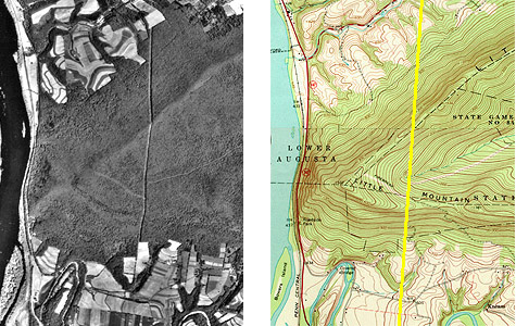
The deformation of the powerline clearing shown in the air photo is caused by relief displacement. (USGS. "Harrisburg East Quadrangle, Pennsylvania")
Below are portions of two aerial photographs showing Little Mountain. The two photos were taken from successive flight paths. The two perspectives can be used to create a stereopair.
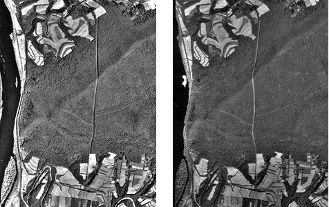
A stereopair: two air photos of the same area taken from different points of view.
Next, the stereopair is superimposed in an anaglyph image. Using your red/blue glasses, you should be able to see a three-dimensional image of Little Mountain in which the power line appears straight, as it would if you were able to see it in person. Notice that the height of Little Mountain is exaggerated due to the fact that the distance between the principal points of the two photos is not exactly proportional to the distance between your eyes.
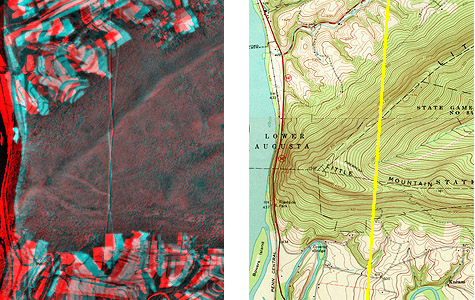
An anaglyph (red/blue) stereo image that fuses the stereopair shown in the above figure. When viewed with a red filter over the left eye and a cyan (blue) filter over the right eye, a sterescopic image is formed. Notice that the powerline clearing, which appears crooked in both air photos, appears straight in the stereoscopic image. (USGS. "Harrisburg East Quadrangle, Pennsylvania")
Let's try that again. We need to make sure that you can visualize how stereoscopic viewing transforms overlapping aerial photographs from perspective views into planimetric views. The aerial photograph and topographic map portions below show the same features, a power line clearing crossing the Sinnemahoning Creek in Central Pennsylvania. The power line appears to bend as it descends to the creek because of relief displacement.
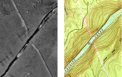
The deformation of the powerline clearing shown in the air photo is caused by relief displacement. (USGS. "Keating Quadrangle, Pennsylvania").
Two aerial photographs of the same area taken from different perspectives constitute a stereo pair.
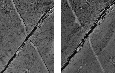
A stereopair, two air photos of the same area taken from different points of view.
By viewing the two photographs stereoscopically, we can transform them from two-dimensional perspective views to a single three-dimensional view in which the geometric distortions caused by relief displacement have been removed.
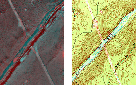
Deformation caused by relief displacement is rectified when the air photos are viewed in stereo. (USGS. "Keating Quadrangle, Pennsylvania").
Photogrammetrists use instruments called stereoplotters to trace, or compile, the data shown on topographic maps from stereoscopic images like the ones you've seen here. The operator pictured below is viewing a stereoscopic model similar to the one you see when you view the anaglyph stereo images with red/blue glasses. A stereopair is superimposed on the right-hand screen of the operator's workstation. The left-hand screen shows dialog boxes and command windows through which she controls the stereoplotter software. Instead of red/blue glasses, the operator is wearing glasses with polarized lens filters that allow her to visualize a three-dimensional image of the terrain. She handles a 3-D mouse that allows her to place a cursor on the terrain image within inches of its actual horizontal and vertical position.

Merri MacKay (graduate of the Penn State Certificate Program in GIS, and employee of BAE Systems ADR), uses an analytic stereoplotter to digitize vertical and horizontal positions from a stereoscopic model. Photo circa 1998, used with permission of Ms. MacKay and ADR, Inc. When she encountered her picture as a student in the class in 2004, Merri wrote "I've got short hair and four grandkids now..."
15. Orthorectification
An orthoimage (or orthophoto) is a single aerial image in which distortions caused by relief displacement have been removed. The scale of an orthoimage is uniform. Like a planimetrically correct map, orthoimages depict scenes as though every point were viewed simultaneously from directly above. In other words, as if every optical axis were orthogonal to the ground surface. Notice how the power line clearing has been straightened in the orthophoto on the right below.
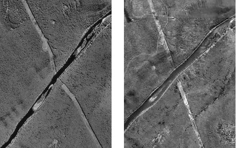
Comparison of a vertical aerial photograph (left) and an orthophoto.
Relief displacement is caused by differences in elevation. If the elevation of the terrain surface is known throughout a scene, the geometric distortion it causes can be rectified. Since photogrammetry can be used to measure vertical as well as horizontal positions, it can be used to create a collection of vertical positions called a terrain model. Automated procedures for transforming vertical aerial photos into orthophotos require digital terrain models.
Since the early 1990s, orthophotos have been commonly used as sources for editing and revising of digital vector data.
16. Metadata
Through the remainder of this Chapter and the next we'll investigate the particular data products that comprise the framework themes of the U.S. National Spatial Data Infrastructure (NSDI). The format I'll use to discuss these data products reflects the Federal Geographic Data Committee's Metadata standard (FGDC, 1998c). Metadata is data about data. It is used to document the content, quality, format, ownership, and lineage of individual data sets. As the FGDC likes to point out, the most familiar example of metadata is the "Nutrition Facts" panel printed on food and drink labels in the U.S. Metadata also provides the keywords needed to search for available data in specialized clearinghouses and in the World Wide Web.
Some of the key headings included in the FGDC metadata standard include:
- Identification Information: Who created the data, a brief description of its content, form, and purpose; its status, spatial extent, and use restrictions;
- Data Quality Information: Accuracy and completeness of attributes, horizontal and vertical positions, sources, and procedures used to create the data;
- Spatial Reference Information: Projection and/or coordinate system; datum and ellipsoid;
- Entity and Attribute Information: Feature and attribute categories used; and
- Distribution Information: Availability, and how to acquire the data.
FGDC's Content Standard for Digital Geospatial Metadata is published at http://www.fgdc.gov/standards/standards_publications/ [44] Geospatial professionals understand the value of metadata, know how to find it, and how to interpret it.
17. Digital Orthophoto Quadrangle (DOQ)
Identification
Digital Orthophoto Quads (DOQs) are raster images of rectified aerial photographs. They are widely used as sources for editing and revising vector topographic data. For example, the vector roads data maintained by businesses like NAVTEQ and Tele Atlas, as well as local and state government agencies, can be plotted over DOQs then edited to reflect changes shown in the orthoimage.
Most DOQs are produced by electronically scanning, then rectifying, black-and-white vertical aerial photographs. DOQ may also be produced from natural-color or near-infrared false-color photos, however, and from digital imagery. The variations in photo scale caused by relief displacement in the original images are removed by warping the image to compensate for the terrain elevations within the scene. Like USGS topographic maps, scale is uniform across each DOQ.
Most DOQs covers 3.75' of longitude by 3.75' of latitude. A set of four DOQs corresponds to each 7.5' quadrangle. (For this reason, DOQs are sometimes called DOQQs--Digital Orthophoto Quarter Quadrangles.) For its National Map, USGS has edge-matched DOQs into seamless data layers, by year of acquisition.

Portion of a USGS Digital Orthophoto Quad (DOQ) for Bushkill, PA.
Data Quality
Like other USGS data products, DOQs conform to National Map Accuracy Standards. Since the scale of the series is 1:12,000, the standards warrant that 90 percent of well-defined points appear within 33.3 feet (10.1 meters) of their actual positions. One of the main sources of error is the rectification process, during which the image is warped such that each of a minimum of 3 control points matches its known location.
Spatial Reference Information
All DOQs are cast on the Universal Transverse Mercator projection used in the local UTM zone. Horizontal positions are specified relative to the North American Datum of 1983, which is based on the GRS 80 ellipsoid.
Entities and Attributes
The fundamental geometric element of a DOQ is the picture element (pixel). Each pixel in a DOQ corresponds to one square meter on the ground. Pixels in black-and-white DOQs are associated with a single attribute: a number from 0 to 255, where 0 stands for black, 255 stands for white, and the numbers in between represent levels of gray.
DOQs exceed the scanned topographic maps shown in Digital Raster Graphics (DRGs) in both pixel resolution and attribute resolution. DOQs are therefore much larger files than DRGs. Even though an individual DOQ file covers only one-quarter of the area of a topographic quadrangle (3.75 minutes square), it requires up to 55 Mb of digital storage. Because they cover only 25 percent of the area of topographic quadrangles, DOQs are also known as Digital Orthophoto Quarter Quadrangles (DOQQs).
Distribution
USGS DOQ files are in the public domain, and can be used for any purpose without restriction. They are available for free download from the USGS at http://earthexplorer.usgs.gov [88]/, or from various state and regional data clearinghouses as well as from the geoCOMMUNITY site http://data.geocomm.com/doqq/ [90] Digital orthoimagery data at 1-foot and 1-meter spatial resolution, collected from multiple sources, are available for user-specified areas from the National Map Viewer site http://nationalmap.gov/ [91] , and even higer resolution imagery (HRO) for certain areas is available through the USGS Seamless Data Warehouse site at http://seamless.usgs.gov/ [92]
To investigate DOQ data in greater depth, including links to a complete sample metadata document, visit http://online.wr.usgs.gov/ngpo/doq/ [93] You're also welcome to post a comment to this page to describe your source of DOQ data, and how you use it. FGDC's Content Standard for Digital Orthoimagery is published at http://www.fgdc.gov/standards/standards_publications/ [44]
| Try This! |
Explore DOQs with Global Mapper (dlgv32 Pro)Now it's time to use Global Mapper (dlgv32 Pro) again, this time to investigate the characteristics of a set of USGS Digital Orthophoto (Quarter) Quadrangles. The instructions below assume that you have already installed the Global Mapper / dlgv32 Pro software on your computer. (If you haven't, return to installation instructions [54] presented earlier in Chapter 6). Note: Global Mapper is a Windows application and will not run under the Macintosh operating system. The questions asked of Penn State students that involve the use of Global Mapper are not graded.
|
| Try This! |
Assess the availability of Digital Orthoimagery via the USGS National Map ViewerThe National Map Viewer is an Internet Map Server application that provides a browsable map interface to the digital data layers that make up the National Map. The orthoimagery available through this interface has been gathered from several sources in addition to the USGS DOQ collection describe above.
|
| Practice Quiz | Registered Penn State students should return now to the Chapter 6 folder in ANGEL (via the Resources menu to the left) to take a self-assessment quiz about Photogrammetry. You may take practice quizzes as many times as you wish. They are not scored and do not affect your grade in any way. |
|
Students who register for this Penn State course gain access to assignments and instructor feedback, and earn academic credit. Information about Penn State's Online Geospatial Education programs is available at http://gis.e-education.psu.edu [1]. |
18. Summary
Many local, state and federal government agencies produce and rely upon geographic data to support their day-to-day operations. The National Spatial Data Infrastructure (NSDI) is meant to foster cooperation among agencies to reduce costs and increase the quality and availability of public data in the U.S. The key components of NSDI include standards, metadata, data, a clearinghouse for data dissemination, and partnerships. The seven framework data themes have been described as "the data backbone of the NSDI" (FGDC, 1997, p. v). This chapter and the next review the origins, characteristics and status of the framework themes. In comparison with some other developed countries, framework data are fragmentary in the U.S., largely because mapping activities at various levels of government remain inadequately coordinated.
Chapter 6 considers two of the seven framework themes: geodetic control and orthoimagery. It discusses the impact of high-accuracy satellite positioning on accuracy standards for the National Spatial Reference System--the U.S.' horizontal and vertical control networks. The chapter stresses the fact that much framework data is derived, directly or indirectly, from aerial imagery. Geospatial professionals understand how photogrammetrists compile planimetrically-correct vector data by stereoscopic analysis of aerial imagery. They also understand how orthoimages are produced and used to help keep vector data current, among other uses.
The most ambitious attempt to implement a nationwide collection of framework data is the USGS' National Map. Composed of some of the digital data products described in this chapter and those that follow, the proposed National Map is to include high resolution (1 m) digital orthoimagery, variable resolution (10-30 m) digital elevation data, vector transportation, hydrography, and boundaries, medium resolution (30 m) land characterization data derived from satellite imagery, and geographic names. These data are to be seamless (unlike the more than 50,000 sheets that comprise the 7.5-minute topographic quadrangle series) and continuously updated. Meanwhile, in 2005, USGS announced that two of its three National Mapping Centers (in Reston, Virginia and Rolla, Missouri) would be closed, and over 300 jobs eliminated. Although funding for the Rolla center was subsequently restored by Congress, it remains to be seen whether USGS will be sufficiently resourced to fulfill its quest for a National Map.
|
Quiz |
Registered Penn State students should return now to the Chapter 6 folder in ANGEL (via the Resources menu to the left) to access the graded quiz for this chapter. This one counts. You may take graded quizzes only once. The purpose of the quiz is to ensure that you have studied the text closely, that you have mastered the practice activities, and that you have fulfilled the chapter's learning objectives. You are welcome to review the chapter during the quiz. Once you have submitted the quiz and posted any questions you may have to either our discussion forums or chapter pages, you will have completed Chapter 6. |
Comments and Questions
Registered students are welcome to post comments, questions, and replies to questions about the text. Particularly welcome are anecdotes that relate the chapter text to your personal or professional experience. In addition, there are discussion forums available in the ANGEL course management system for comments and questions about topics that you may not wish to share with the whole world.
To post a comment, scroll down to the text box under "Post new comment" and begin typing in the text box, or you can choose to reply to an existing thread. When you are finished typing, click on either the "Preview" or "Save" button (Save will actually submit your comment). Once your comment is posted, you will be able to edit or delete it as needed. In addition, you will be able to reply to other posts at any time.
Note: the first few words of each comment become its "title" in the thread.
|
Students who register for this Penn State course gain access to assignments and instructor feedback, and earn academic credit. Information about Penn State's Online Geospatial Education programs is available at http://gis.e-education.psu.edu [1]. |
19. Bibliography
Anson, A. (2002) Topographic mapping with plane table and alidade in the 1940s. [CD-ROM] Professional Surveyors Publishing Co.
Doyle, David R. 1994 Development of the national spatial reference system. Retrieved 9 November 2007 from http://www.ngs.noaa.gov/PUBS_LIB/develop_NSRS.html [18]
Federal Geodetic Control Committee (1988). Geometric geodetic accuracy standards and specifications for using GPS relative positioning techniques. Retrieved February 11, 2008, from http://www.ngs.noaa.gov/FGCS/tech_pub/GeomGeod.pdf [19]
Federal Geographic Data Committee (1998a). Geospatial positing accuracy standards part 2: standards for geodetic networks. Retrieved February 11, 2008, from http://www.fgdc.gov/standards/standards_publications/ [44]
Federal Geographic Data Committee (1998b). Geospatial positing accuracy standards part 1: reporting methodology. Retrieved February 11, 2008, from http://www.fgdc.gov/standards/standards_publications/ [44]
Federal Geographic Data Committee (1998c). Content standard for digital geospatial metadata. Retrieved February 19, 2008, from http://www.fgdc.gov/standards/standards_publications/ [44]
Gidon, P. (2006). Alpes_stereo. Retrieved May 10, 2006, from http://perso.infonie.fr/alpes_stereo/i_index.htm [98] (Expired link.)
Masser, I. (1998). Governments and geographic information. London: Taylor & Francis.
Moore, Larry (2000) The U.S. Geological Survey's revision program for 7.5-Minute topographic maps. Retrieved December 14, 2007 from http://pubs.usgs.gov/of/2000/of00-325/moore.html [99]
National Aeronautic and Space Administration (1997). Mars pathfinder. Retrieved June 7, 2006, from http://mars.jpl.nasa.gov/MPF/index0.html [100]
National Geodetic Survey (2007). The National Geodetic Survey 10 year plan; mission, vision and strategy 2007-2017. Retrieved February 19, 2008 from www.ngs.noaa.gov/INFO/ngs_tenyearplan.pdf [101]
National Oceanic and Atmospheric Administration (2007) NOAA history. Retrieved February 18, 2008, from http://www.history.noaa.gov/ [77]
National Research Council (2002). Research opportunities in geography at the U.S. Geological Survey. Washington DC: National Academies Press.
National Research Council (2007). A research agenda for geographic information science at the United States Geological Survey. Washington DC: National Academies Press.
Office of Management and Budget (1990) Circular A-16, revised. Retrieved February 19, 2008, from http://www.whitehouse.gov/omb/circulars_a016_rev [102]
Parry, R.B. (1987). The state of world mapping. In R. Parry & C. Perkins (Eds.), World mapping today. Butterworth-Heinemann.
Robinson, A. et al. (1995). Elements of cartography (5th ed.). New York: John Wiley & Sons.
Thompson, M. M. (1988). Maps for America, cartographic products of the U.S. geological survey and others (3d ed.). Reston, Va.: U.S. Geological Survey.
United States Geological Survey (2001). The National Map: topographic mapping for the 21st century. Final Report, November 30. Retrieved 11 January 2008 from http://nationalmap.gov/report/national_map_report_final.pdf [103]
White House (1994) Executive order 12906: coordinating geographic data access. Retrieved February 19, 2008, from http://www.fgdc.gov/policyandplanning/executive_order [104]
NEW Chapter 8: Imaging our World
Chapter 9 *old*: Geoanalytics: From Data to Answers (LLRW)
1. Overview
Geographic data are expensive to produce and maintain. Data often accounts for the lion's share of the cost of building and running geographic information systems. The expense of GIS is justifiable when it gives people the information they need to make wise choices in the face of complex problems. In this chapter we'll consider one such problem: the search for suitable and acceptable sites for low level radioactive waste disposal facilities. Two case studies will demonstrate that GIS is very useful indeed for assimilating the many site suitability criteria that must be taken into account, provided that the necessary data can be assembled in a single, integrated system. The case studies will allow us to compare vector and raster approaches to site selection problems.
The ability to integrate diverse geographic data is a hallmark of mature GIS software. The know-how required to accomplish data integration is also the mark of a truly knowledgeable GIS user. What knowledgeable users also recognize, however, is that while GIS technology is well suited to answering certain well defined questions, it often cannot help resolve crucial conflicts between private and public interests. The objective of this final, brief chapter is to consider the challenges involved in using GIS to address a complex problem that has both environmental and social dimensions. Specifically, in this chapter you will learn to:
Objectives
Chapter 9 should help prepare you to:
- Recognize the characteristics of geographic data that must be taken into account to overlay multiple data layers;
- Compare and contrast vector and raster approaches to site suitability studies;
- Have realistic expectations about what geographic data analysis can achieve.
Comments and Questions?
Registered students are welcome to post comments, questions, and replies to questions about the text. Particularly welcome are anecdotes that relate the chapter text to your personal or professional experience. In addition, there are discussion forums available in the ANGEL course management system for comments and questions about topics that you may not wish to share with the whole world.
To post a comment, scroll down to the text box under "Post new comment" and begin typing in the text box, or you can choose to reply to an existing thread. When you are finished typing, click on either the "Preview" or "Save" button (Save will actually submit your comment). Once your comment is posted, you will be able to edit or delete it as needed. In addition, you will be able to reply to other posts at any time.
Note: the first few words of each comment become its "title" in the thread.
|
Students who register for this Penn State course gain access to assignments and instructor feedback, and earn academic credit. Information about Penn State's Online Geospatial Education programs is available at http://gis.e-education.psu.edu [1]. |
2. Checklist
The following checklist is for Penn State students who are registered for classes in which this text, and associated quizzes and projects in the ANGEL course management system, have been assigned. You may find it useful to print this page out first so that you can follow along with the directions.
Chapter 9 Checklist (for registered students only) |
||
| Step | Activity | Access/Directions |
|---|---|---|
| 1 | Read Chapter 9 | This is the second page of the Chapter. Click on the links at the bottom of the page to continue or to return to the previous page, or to go to the top of the chapter. You can also navigate the text via the links in the GEOG 482 menu on the left. |
| 2 | Chapter 9 includes no practice quizzes. | |
| 3 | Perform "Try this" activities including:
"Try this" activities are not graded. |
Instructions are provided for each activity. |
| 4 | Submit the Chapter 9 Graded Quiz | ANGEL > [your course section] > Lessons tab > Chapter 9 folder > Chapter 9 Graded Quiz. See the Calendar tab in ANGEL for due dates. |
| 5 | Read comments and questions posted by fellow students. Add comments and questions of your own, if any. | Comments and questions may be posted on any page of the text, or in a Chapter-specific discussion forum in ANGEL. |
3. Context
This section sets a context for two case studies that follow. First, I will briefly define low level radioactive waste (LLRW). Then I discuss the legislation that mandated construction of a dozen or more regional LLRW disposal facilities in the U.S. Finally, I will reflect briefly on how the capability of geographic information systems to integrate multiple data "layers" is useful for siting problems like the ones posed by LLRW.
4. Low Level Radioactive Waste
According to the U.S. Nuclear Regulatory Commission (2004), LLRW consists of discarded items that have become contaminated with radioactive material or have become radioactive through exposure to neutron radiation. Trash, protective clothing, and used laboratory glassware make up all but about 3 percent of LLRW. These "Class A" wastes remain hazardous less than 100 years. "Class B" wastes, consisting of water purification filters and ion exchange resins used to clean contaminated water at nuclear power plants, remain hazardous up to 300 years. "Class C" wastes, such as metal parts of decommissioned nuclear reactors, constitute less than 1 percent of all LLRW, but remain dangerous for up to 500 years.
The danger of exposure to LLRW varies widely according to the types and concentration of radioactive material contained in the waste. Low level waste containing some radioactive materials used in medical research, for example, is not particularly hazardous unless inhaled or consumed, and a person can stand near it without shielding. On the other hand, exposure to LLRW contaminated by processing water at a reactor can lead to death or an increased risk of cancer (U.S. Nuclear Regulatory Commission, n.d.).
Production trends and destinations of low level radioactive waste. (U.S. Nuclear Regulatory Commission, 2005).
Hundreds of nuclear facilities across the country produce LLRW, but only a very few disposal sites are currently willing to store it. Disposal facilities at Clive, Utah, Barnwell, South Carolina, and Richland, Washington, accepted over 4,000,000 cubic feet of LLRW in both 2005 and 2006, up from 1,419,000 cubic feet in 1998. By 2008 the volume had dropped to just over 2,000,000 cubic feet (U.S. Nuclear Regulatory Commisssion, 2011a). Sources include nuclear reactors, industrial users, government sources (other than nuclear weapons sites), and academic and medical facilities. (We have a small nuclear reactor here at Penn State that is used by students in graduate and undergraduate nuclear engineering classes.)
5. Siting LLRW Storage Facilities
The U.S. Congress passed the Low Level Radioactive Waste Policy Act in 1980. As amended in 1985, the Act made states responsible for disposing of the LLRW they produce. States were encouraged to form regional "compacts" to share the costs of locating, constructing, and maintaining LLRW disposal facilities. The intent of the legislation was to avoid the very situation that has since come to pass, that the entire country would become dependent on a very few disposal facilities.

Regional compacts formed by states in response to the LLRW Policy Act (U.S. Nuclear Regulatory Commission, 2011b).
State government agencies and the consultants they hire to help select suitable sites assume that few if any municipalities would volunteer to host a LLRW disposal facility. They prepare for worst-case scenarios in which states would be forced to exercise their right of eminent domain to purchase suitable properties without the consent of landowners or their neighbors. GIS seems to offer an impartial, scientific, and therefore defensible approach to the problem. As Mark Monmonier has written, "[w]e have to put the damned thing somewhere, the planners argue, and a formal system of map analysis offers an 'objective,' logical method for evaluating plausible locations" (Monmonier, 1995, p. 220). As we discussed in our very first chapter, site selection problems pose a geographic question that geographic information systems are well suited to address, namely, which locations have attributes that satisfy all suitability criteria?
6. Map Overlay Concept
Environmental scientists and engineers consider many geological, climatological, hydrological, and surface and subsurface land use criteria to determine whether a plot of land is suitable or unsuitable for a LLRW facility. Each criterion can be represented with geographic data, and visualized as a thematic map. In theory, the site selection problem is as simple as compiling onto a single map all the disqualified areas on the individual maps, and then choosing among whatever qualified locations remain. In practice, of course, it is not so simple.
There is nothing new about superimposing multiple thematic maps to reveal optimal locations. One of the earliest and most eloquent descriptions of the process was written by Ian McHarg, a landscape architect and planner, in his influential book Design With Nature. In a passage describing the process he and his colleagues used to determine the least destructive route for a new roadway, McHarg (1971) wrote:
...let us map physiographic factors so that the darker the tone, the greater the cost. Let us similarly map social values so that the darker the tone, the higher the value. Let us make the maps transparent. When these are superimposed, the least-social-cost areas are revealed by the lightest tone. (p. 34).
As you probably know, this process has become known as map overlay. Storing digital data in multiple "layers" is not unique to GIS, of course; computer-aided design (CAD) packages and even spreadsheets also support layering. What's unique about GIS, and important about map overlay, is its ability to generate a new data layer as a product of existing layers. In the example illustrated below, for example, analysts at Penn State's Environmental Resources Research Institute estimated the agricultural pollution potential of every major watershed in the state by overlaying watershed boundaries, the slope of the terrain (calculated from USGS DEMs), soil types (from U.S. Soil Conservation Service data), land use patterns (from the USGS LULC data), and animal loading (livestock wastes estimated from the U.S. Census Bureau's Census of Agriculture).
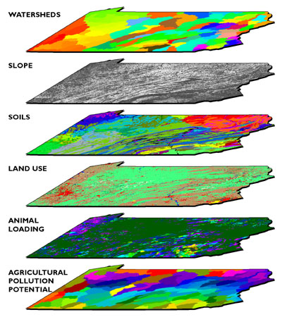
Diagram illustrating the map overlay process used to evaluate potential agricultural pollution by watershed in Pennsylvania.
As illustrated below, map overlay can be implemented in either vector or raster systems. In the vector case, often referred to as polygon overlay, the intersection of two or more data layers produces new features (polygons). Attributes (symbolized as colors in the illustration) of intersecting polygons are combined. The raster implementation (known as grid overlay) combines attributes within grid cells that align exactly. Misaligned grids must be resampled to common formats.
Map overlay is a procedure for combining the attributes of intersecting features that are represented in two or more georegistered data layers.
Polygon and grid overlay procedures produce useful information only if they are performed on data layers that are properly georegistered. Data layers must be referenced to the same coordinate system (e.g., the same UTM and SPC zones), the same map projection (if any), and the same datum (horizontal and vertical, based upon the same reference ellipsoid). Furthermore, locations must be specified with coordinates that share the same unit of measure.
7. Pennsylvania Case Study
In response to the LLRW Policy Act, Pennsylvania entered into an "Appalachian Compact" with the states of Delaware, Maryland, and West Virginia to share the costs of siting, building, and operating a LLRW storage facility. Together, these states generated about 10 percent of the total volume of LLRW then produced in the U.S. Pennsylvania, which generated about 70 percent of the total produced by the Appalachian Compact, agreed to host the disposal site.
In 1990, the Pennsylvania Department of Environmental Protection commissioned Chem-Nuclear Systems Incorporated (CNSI) to identify three potentially suitable sites to accommodate two to three truckloads of LLRW per day for 30 years. CNSI, the operator of the Barnwell South Carolina site, would also operate the Pennsylvania site for profit.
Sketch of the proposed Pennsylvania LLRW disposal facility (Pennsylvania Department of Environmental Protection, 1998).
CNSI's plan called for storing LLRW in 55-gallon drums encased in concrete, buried in clay, surrounded by a polyethylene membrane. The disposal facilities, along with support and administration buildings and a visitors center, would occupy about 50 acres in the center of a 500-acre site. (Can you imagine a family outing to the Visitors Center of a LLRW disposal facility?) The remaining 450 acres would be reserved for a 500 to 1000 foot wide buffer zone.
The three stage siting process agreed to by CNSI and the Pennsylvania Department of Environmental Protection corresponded to three scales of analysis: statewide, regional, and local. All three stages relied on vector geographic data integrated within a GIS.
8. Vector Approach
CNSI and its subcontractors adopted a vector approach for its GIS-based site selection process. When the process began in 1990, far less geographic data was available in digital form than it is today. Most of the necessary data was available only as paper maps, which had to be converted to digital form. In one of its interim reports, CNSI described two digitizing procedures used, "digitizing" and "scanning." Here's how it described "digitizing:"
In the digitizing process, a GIS operator uses a hand-held device, known as a cursor, to trace the boundaries of selected disqualifying features while the source map is attached to a digitizing table. The digitizing table contains a fine grid of sensitive wire imbedded within the table top. This grid allows the attached computer to detect the position of the cursor so that the system can build an electronic map during the tracing. In this project, source maps and GIS-produced maps were compared to ensure that the information was transferred accurately. (Chem Nuclear Systems, 1993, p. 8).
One aspect overlooked in the CNSI description is that operators must encode the attributes of features as well as their locations. Some of you know all too well that tablet digitizing (illustrated in the photo below left) is an extraordinarily tedious task, so onerous that even student interns resent it. One wag here at Penn State suggested that the acronym "GIS" actually stands for "Getting it (the data) In Stinks." You can substitute your own "S" word if you wish.
Vector digitizing with a tablet (left); raster digitizing with a drum scanner (right) (USGS).
Compared to the drudgery of tablet digitizing, electronically scanning paper maps seems simple and efficient. Here's how CNSI describes it:
The scanning process is more automated than the digitizing process. Scanning is similar to photocopying, but instead of making a paper copy, the scanning device creates an electronic copy of the source map and stores the information in a computer record. This computer record contains a complete electronic picture (image) of the map and includes shading, symbols, boundary lines, and text. A GIS operator can select the appropriate feature boundaries from such a record. Scanning is useful when maps have very complex boundaries lines that can not be easily traced. (Chem Nuclear Systems, Inc., 1993, p. 8)
I hope you noticed that CNSI's description glosses over the distinction between raster and vector data. If scanning is really as easy as they suggest, why would anyone ever tablet-digitize anything? In fact, it is not quite so simple to "select the appropriate feature boundaries" from a raster file, which is analogous to a remotely sensed image. The scanned maps had to be transformed from pixels to vector features using a semi-automated procedure called raster to vector conversion, otherwise known as "vectorization." Time-consuming manual editing is required to eliminate unwanted features (like vectorized text), correct digital features that were erroneously attached or combined, and to identify the features by encoding their attributes in a database.
In either the vector or raster case, if the coordinate system, projection, and datums of the original paper map were not well defined, the content of the map first had to be redrawn, by hand, onto another map whose characteristics are known.
9. Stage One: Statewide Screening
CNSI considered several geological, hydrological, surface and subsurface land use criteria in the first stage of its LLRW siting process. [View a table that lists all the Stage One criteria [105].] CNSI's GIS subcontractors created separate digital map layers for every criterion. Sources and procedures used to create three of the map layers are discussed briefly below.
Areas underlain by limestone and other carbonate rocks were digitized from the Pennsylvania Geological Survey's Geologic Map of Pennsylvania. (Chem-Nuclear Systems, 1991).
One of the geological criteria considered was carbonate lithology. Limestone and other carbonate rocks are permeable. Permeable bedrock increases the likelihood of ground water contamination in the event of a LLRW leak. Areas with carbonate rock outcrops were therefore disqualified during the first stage of the screening process. Boundaries of disqualified areas were digitized from the 1:250,000-scale Geologic Map of Pennsylvania (1980). What concerns would you have about data quality given a 1:250,000-scale source map?
Coastal flood plains were digitized from 100-year flood contours compiled from FEMA Flood Insurance Rate Maps onto USGS topographic maps. (Chem-Nuclear Systems, 1991).
Analysts needed to make sure that the LLRW disposal facility would never be inundated with water in the event of a coastal flood, or a rise in sea level. To determine disqualified areas, CNSI's subcontractors relied upon the Federal Emergency Management Agency's Flood Insurance Rate Maps (FIRMs). The maps were not available in digital form at the time, and did not include complete metadata. According to the CNSI interim report, "[t]he 100-year flood plains shown on maps obtained from FEMA ... were transferred to USGS 7.5-minute quad sheet maps. The 100-year flood plain boundaries were digitized into the GIS from the 7.5-minute quad sheet maps." (Chem Nuclear Systems, 1991, p. 11) Why would the contractors go to the trouble of redrawing the floodplain boundaries onto topographic maps prior to digitizing?
"Exceptional value watersheds" were delineated on topographic maps, then digitized. (Chem-Nuclear Systems, 1991).
Areas designated as "exceptional value watersheds" were also disqualified during Stage One. Pennsylvania legislation protected 96 streams. Twenty-nine additional streams were added during the site screening process. "The watersheds were delineated on county [1:50,000 or 1:100,000-scale topographic] maps by following the appropriate contour lines. Once delineated, the EV stream and its associated watershed were digitized into the GIS." (Chem Nuclear Systems, 1991, p. 12) What digital data sets could have been used to delineate the watersheds automatically, had the data been available?
After all the Stage One maps were digitized, georegistered, and overlayed, approximately 23 percent of the state's land area was disqualified.
10. Stage Two: Regional Screening
CNSI considered additional disqualification criteria during the second, "regional" stage of the LLRW siting process. [View a table that lists all the Stage Two criteria [106].] Some of the Stage Two criteria had already been considered during Stage One, but were now reassessed in light of more detailed data compiled from larger-scale sources. In its interim report, CNSI had this to say about the composite disqualification map shown below:
When all the information was entered in to Stage Two database, the GIS was used to draw the maps showing the disqualified land areas. ... The map shows both additions/refinements to the Stage One disqualifying features and those additional disqualifying features examined during Stage Two. (Chem Nuclear Systems, 1993, p. 19)
Composite map showing approximately 46 per cent of the state disqualified as a result of Stages One and Two of the LLRW site selection process. (Chem-Nuclear Systems, 1993).
CNSI added this disclaimer:
The Stage Two Disqualifying maps found in Appendix A depict information at a scale of 1:1.5 million. At this scale, one inch on the map represents 24 miles, or one mile is represented on the map by approximately four one-hundreds of an inch. A square 500-acre area measures less than one mile on a side. Printing of such fine detail on the 11" × 17" disqualifying maps was not possible, therefore, it is possible that small areas of sufficient size for the LLRW disposal facility site may exist within regions that appear disqualified on the attached maps. [Emphasis in the original document] The detailed boundary information for these small areas is retained within the GIS even though they are not visually illustrated on the maps. (Chem Nuclear Systems, 1993, p. 20)
As I mentioned back in Chapter 2, CNSI representatives took some heat about the map scale problem in public hearings. Residents took little solace in the assertion that the data in the GIS were more truthful than the data depicted on the map.
11. Stage Three: Local Disqualification
Many more criteria were considered in Stage Three. [View a table that lists all the Stage Three criteria [107].] At the completion of the third stage, roughly 75 percent of the state's land area had been disqualified.
One of the new criteria introduced in Stage Three was slope. Analysts were concerned that precipitation runoff, which increases as slope increases, might increase the risk of surface water contamination should the LLRW facility spring a leak. CNSI's interim report (1994a) states that "[t]he disposal unit area which constitutes approximately 50 acres ... may not be located where there are slopes greater than 15 percent as mapped on U.S. Geological Survey (USGS) 7.5-minute quadrangles utilizing a scale of 1:24,000 ..." (p. 9).
Slope is change in terrain elevation over a given horizontal distance. It is often expressed as a percentage. A 15 percent slope changes at a rate of 15 feet of elevation for every 100 feet of horizontal distance. Slope can be measured directly on topographic maps. The closer the spacing of elevation contours, the greater the slope. CNSI's GIS subcontractors were able to identify areas with excessive slope on topographic maps using plastic templates called "land slope indicators" that showed the maximum allowable contour spacing.
Fortunately for the subcontractors, 7.5-minute USGS DEMs were available for 85 percent of the state (they're all available now). Several algorithms have been developed to calculate slope at each grid point of a DEM. As described in chapter 7, the simplest algorithm calculates slope at a grid point as a function of the elevations of the eight points that surround it to the north, northeast, east, southeast, and so on. CNSI's subcontractors used GIS software that incorporated such an algorithm to identify all grid points whose slopes were greater than 15 percent. The areas represented by these grid points were then made into a new digital map layer.
| Try This! |
You can create a slope map of the Bushkill PA quadrangle with Global Mapper (dlgv32 Pro) software.
By default, pixels with 0 percent slope are lightest, and pixels with 30 percent slope or more are darkest. You can adjust this at Tools > Configure > Shader Options. Notice that the slope symbolization does not change even as you change the vertical exaggeration of the DEM (Tools > Configure > Vertical Options). |
|
Students who register for this Penn State course gain access to assignments and instructor feedback, and earn academic credit. Information about Penn State's Online Geospatial Education programs is available at http://gis.e-education.psu.edu [1]. |
12. Buffering
Several of the disqualification criteria involve buffer zones. For example, one disqualifying criterion states that "[t]he area within 1/2 mile of an existing important wetland ... is disqualified." Another states that "disposal sites may not be located within 1/2 mile of a well or spring which is used as a public water supply." (Chem-Nuclear Systems, 1994b). As I mentioned in the chapter 1 (and as you may know from experience), buffering is a GIS procedure by which zones of specified radius or width are defined around selected vector features or raster grid cells.
Like map overlay, buffering has been implemented in both vector and raster systems. The vector implementation involves expanding a selected feature or features, or producing new surrounding features (polygons). The raster implementation accomplishes the same thing, except that buffers consist of sets of pixels rather than discrete features.
Buffer zones (yellow) surround vector and raster representations of a pond and stream.
13. New York Case Study
Like Pennsylvania, the State of New York was compelled by the LLRW Policy Act to dispose of its waste within its own borders. New York also turned to GIS in the hope of finding a systematic and objective means of determining an optimal site. Instead of the vector approach used by its neighbor, however, New York opted for a raster framework.
Overview of the raster approach adopted by the New York LLRW Siting Commission, part one. (Monmonier, 1995).
Mark Monmonier, a professor of geography at Syracuse University (and a Penn State alumnus), has written that the list of siting criteria assembled by the New York Department of Environmental Conservation (DEC) was "an astute mixture of common sense, sound environmental science, and interest-group politics" (1995, p. 226). Source data included maps and attribute data produced by the U.S. Census Bureau, the New York Department of Transportation, and the DEC itself, among others. The New York LLRW Siting Commission overlaid the digitized source maps with a grid composed of cells that corresponded to one square mile (640 acres; slightly larger than the 500 acres required for a disposal site) on the ground. As illustrated above, the Siting Commission's GIS subcontractors then assigned each of the 47,224 grid cells a "favorability" score for each criterion. The process was systematic, but hardly objective, since the scores reflected social values (to borrow the term used by McHarg).
Overview of the raster approach adopted by the New York LLRW Siting Commission, part two. (Monmonier, 1995).
To acknowledge the fact that some criteria were more important than others, the Siting Commission weighted the scores in each data layer by multiplying them all by a constant factor. Like the original integer scores, the weighting factors were a negotiated product of consensus, not of objective measurement. Finally, the commission produced a single set of composite scores by summing the scores of each raster cell through all the data layers. A composite favorability map could then be produced from the composite scores. All that remained was for the public to embrace the result.
14. Outcomes
To date, neither Pennsylvania nor New York has built a LLRW disposal facility. Both states gave up on their unpopular siting programs shortly after Republicans replaced Democrats in the 1994 gubernatorial elections.
The New York process was derailed when angry residents challenged proposed sites on account of inaccuracies discovered in the state's GIS data, and because of the state's failure to make the data accessible for citizen review in accordance with the Freedom of Information Act (Monmonier, 1995).
Pennsylvania's $37 million siting effort succeeded in disqualifying more than three quarters of the state's land area, but failed to recommend any qualified 500-acre sites. With the volume of its LLRW decreasing, and the Barnwell South Carolina facility still willing to accept Pennsylvania's waste shipments, the search was suspended "indefinitely" in 1998.
To fulfill its obligations under the LLRW Policy Act, Pennsylvania has initiated a "Community Partnering Plan" that solicits volunteer communities to host a LLRW disposal facility in return for jobs, construction revenues, shares of revenues generated by user fees, property taxes, scholarships, and other benefits. The plan has this to say about the GIS site selection process that preceded it: "The previous approach had been to impose the state's will on a municipality by using a screening process based primarily on technical criteria. In contrast, the Community Partnering Plan is voluntary." (Chem Nuclear Systems, 1996, p. 3)
The New York and Pennsylvania state governments turned to GIS because it offered an impartial and scientific means to locate a facility that nobody wanted in their backyard. Concerned residents criticized the GIS approach as impersonal and technocratic. There is truth to both points of view. Specialists in geographic information need to understand that while GIS can be effective in answering certain well-defined questions, it does not ease the problem of resolving conflicts between private and public interests.
Meanwhile, a Democrat replaced a Republican as governor of South Carolina in 1998. The new governor warned that the Barnwell facility might not continue to accept out-of-state LLRW. "We don't want to be labeled as the dumping ground for the entire country," his spokesperson said (Associated Press, 1998).
No volunteer municipality has yet come forward in response to Pennsylvania's Community Partnering Plan. If the South Carolina facility does stop accepting Pennsylvania's LLRW shipments, and if no LLRW disposal facility is built within the state's borders, then nuclear power plants, hospitals, laboratories, and other facilities may be forced to store LLRW on site. It will be interesting to see if the GIS approach to site selection is resumed as a last resort, or if the state will continue to up the ante in its attempts to attract volunteers, in the hope that every municipality has its price. If and when a volunteer community does come forward, detailed geographic data will be produced, integrated, and analyzed to make sure that the proposed site is suitable after all.
| Try This! | To find out about LLRW-related activities where you live, use your favorite search engine to search the Web on "Low-Level Radioactive Waste [your state or area of interest]". If GIS is involved in your state's LLRW disposal facility site selection process, your state agency that is concerned with environmental affairs is likely to be involved. Add a comment to this page to share your discovery. |
|
Students who register for this Penn State course gain access to assignments and instructor feedback, and earn academic credit. Information about Penn State's Online Geospatial Education programs is available at http://gis.e-education.psu.edu [1]. |
15. Conclusion
Site selection projects like the ones discussed in this chapter require the integration of diverse geographic data. The ability to integrate and analyze data organized in multiple thematic layers is a hallmark of geographic information systems. To contribute to GIS analyses like these, you need to be both a knowledgeable and skillful GIS user. The objective of this text, and the associated Penn State course, has been to help you become more knowledgeable about geographic data.
Knowledgeable users are well versed in the properties of geographic data that need to be taken into account to make data integration possible. Knowledgeable users understand the distinction between vector and raster data, and know something about how features, topological relationships among features, attributes, and time can be represented within the two approaches. Knowledgeable users understand that in order for geographic data to be organized and analyzed as layers, the data must be both orthorectified and georegistered. Knowledgeable users look out for differences in coordinate systems, map projections, and datums that can confound efforts to georegister data layers. Knowledgeable users know that the information needed to register data layers is found in metadata.
Knowledgeable users understand that all geographic data are generalized, and that the level of detail preserved depends upon the scale and resolution at which the data were originally produced. Knowledgeable users are prepared to convince their bosses that small-scale, low resolution data should not be used for large-scale analyses that require high resolution results. Knowledgeable users never forget that the composition of the Earth's surface is constantly changing, and that unlike fine wine, the quality of geographic data does not improve over time.
Knowledgeable users are familiar with the characteristics of the "framework" data that make up the U.S. National Spatial Data Infrastructure, and and are able to determine whether these data are available for a particular location. Knowledgeable users recognize situations in which existing data are inadequate, and when new data must be produced. They are familiar enough with geographic information technologies such as GPS, aerial imaging, and satellite remote sensing that they can judge which technology is best suited to a particular mapping problem.
And knowledgeable users know what kinds of questions GIS is, and is not, suited to answer.
| Quiz |
Registered Penn State students should return now to the Chapter 9 folder in ANGEL (via the Resources menu to the left) to take the Chapter 9 graded quiz. (Note that this brief chapter included no practice quizzes.) You may take graded quizzes only once. The purpose of the quiz is to ensure that you have studied the text closely, that you have mastered the practice activities, and that you have fulfilled the chapter's learning objectives. You are free to review the chapter during the quiz. Once you have submitted the quiz and posted any questions you may have to either our discussion forums or chapter pages, you will have completed Chapter 9. |
Comments and Questions
Registered students are welcome to post comments, questions, and replies to questions about the text. Particularly welcome are anecdotes that relate the chapter text to your personal or professional experience. In addition, there are discussion forums available in the ANGEL course management system for comments and questions about topics that you may not wish to share with the whole world.
To post a comment, scroll down to the text box under "Post new comment" and begin typing in the text box, or you can choose to reply to an existing thread. When you are finished typing, click on either the "Preview" or "Save" button (Save will actually submit your comment). Once your comment is posted, you will be able to edit or delete it as needed. In addition, you will be able to reply to other posts at any time.
Note: the first few words of each comment become its "title" in the thread.
|
|
Students who register for this Penn State course gain access to assignments and instructor feedback, and earn academic credit. Information about Penn State's Online Geospatial Education programs is available at http://gis.e-education.psu.edu [1]. |
16. Bibliography
Associated Press (1998). South Carolina Says Pennsylvania Waste Not Wanted in State. Centre Daily Times, , November 28, pp. 1A.
Chem-Nuclear Systems, Inc. (1991). Pennsylvania low-level radioactive waste disposal facility site screening interim report, stage one -- Statewide disqualification. Harrisburg, PA.
Chem-Nuclear Systems Inc (1993). Pennsylvania low-level radioactive waste disposal facility site screening interim report stage two -- Regional disqualification. Harrisburg PA.
Chem-Nuclear Systems, Inc. (1994a). Pennsylvania low-level radioactive waste disposal facility site screening interim report, stage three -- local disqualification. Harrisburg PA.
Chem-Nuclear Systems, Inc. (1994b). Site selection manual. S80-PL-007, Rev. 0
Chem-Nuclear Systems Inc. (1996). Community partnering plan: Pennsylvania low-level radioactive waste disposal facility. S80-PL-021, Rev. 0.
Chrisman, N. (1997). Exploring geographic information systems. New York: John Wiley & Sons.
McHarg, I. (1971). Design with nature. New York: Doubleday / Natural History Press.
Mertz, T. (1993). GIS targets agricultural nonpoint pollution. GIS World, April, 41-46.
Monmonier, M. (1995). Drawing the line: Tales of maps and carto-controversy. New York: Henry Holt.
Pennsylvania Department of Environmental Protection. (1998). Proposed model of the PA low-level radioactive waste disposal facility.
U.S. Nuclear Regulatory Commission. (n. d.). Radioactive waste: Production, storage, disposal (Report NUREG/BR-0216).
U.S. Nuclear Regulatory Commission. (2005). Radioactive Waste Statistics. Retrieved May 14, 2006, from http://www.nrc.gov/waste/llw-disposal/statistics.html [108] (expired)
U.S. Nuclear Regulatory Commission. (2011a). Low-Level Waste Disposal Statistics. Retrieved November 30, 2011, from http://www.nrc.gov/waste/llw-disposal/licensing/statistics.html [109]
U.S. Nuclear Regulatory Commission. (2011b). Low-Level Waste Compacts. Retrieved November 30, 2011, from [108]http://www.nrc.gov/waste/llw-disposal/licensing/compacts.html [110]