In Chapter 1, we discussed how geographic data rely on locational attributes and provided several examples demonstrating the importance of “place” in GIScience. One of the fastest growing uses of place information is for Location-Based Services (LBS) that take advantage of your phone’s ability to determine your location and, from that location, identify a wide array of nearby “services.” Using your smartphone to check in to your favorite restaurant would do very little if the device had no way to ‘know’ you were in the restaurant. Similarly, your phone could not help you find the nearest gas station while on a trip without knowing where you are at the time.

So, how does this happen - how does your phone know where you are? How can a radio collar detect a grizzly bear’s position and report it back to interested rangers? What, if anything, causes GPS to not work, and how can positional errors be corrected? This chapter will answer these questions and introduce the methods that make these technologies and processes possible.

Although tremendous technological advancements have occurred in the last century, the methods used to determine one’s position on the Earth pre-date satellites, the Internet, and smartphones. Readers of this chapter will trace the history of these technologies back to their foundations in land surveying and triangulation, acquiring knowledge about our incredible technologies and the basic concepts that drive them.

Objectives

Students who successfully complete Chapter 5 should be able to:

1. identify and define the key aspects of geographic data quality, including resolution, precision, and accuracy;
2. explain how radio signals broadcast by Global Positioning System (GPS) satellites are used to calculate positions on the surface of the Earth;
3. state the kinds and magnitude of error associated with uncorrected GPS positioning;
4. identify and explain methods used to improve the accuracy of GPS positioning;
5. list and explain the procedures land surveyors use to produce positional data, including traversing, triangulation, and trilateration.

Table of Contents

• Geospatial Data Quality:Validity, Accuracy, and Precision
• Global Positioning Systems
• GPS Error Sources
• Correcting GPS Errors
• Land Surveying and Conventional Techinques for Measuring Positions on the Earth's Surface
• Summary
• Glossary
• Biblography

5.1.1 Validity

Data are not created equal; data vary in their quality. Data quality is a concept with multiple components that include ideas of data precision and accuracy, thus a focus on whether the data are specific enough and how much error they contain. Data quality also includes data relevance, which determines whether or not the data are suitable for a particular application. Aspects of data quality are often characterized overall as “fitness for use.” The degree to which data are fit for an application can be affected by a number of characteristics, ranging from discrepancies and inconsistencies in the formatting of the data to the data being of the wrong type or having too many errors.

Imagine you’re one of the interested rangers tracking grizzly bears through a wildlife refuge in an attempt to identify areas where the public might come into contact with the animals. Radio collars worn by the bears are sending new locational data every five minutes, and with each update, the bears’ activity patterns become evident. In this instance, there are no problems with data validity: you are interested in the bears’ positions, and that is exactly the data your tracking equipment is receiving.

Since these fictional, error-free tracking data are perfectly relevant for the problem at hand, there is no need to consider alternative data. The data quality is clearly high enough for the purpose at hand.

Data with quality this high in relation to the purpose is not the norm, nor is it always needed. Often, we must make very careful decisions about which data to use and why one set of data may be better than another. Rather than knowing the precise location of every bear in the refuge, a much more likely scenario would involve rangers relying on one or more of the other databases they may have; their available databases might include: trapping records, reported bear sightings by guests, veterinary logs, and sales from the visitor center.

Although the sales records from the visitor center could be disregarded as not suitable for the purpose at hand, the other data are all potentially relevant. In this case, the rangers would have to decide which database, or combination of databases, would be the best fit for the task of identifying park locations where restrictions on public access might be needed to prevent close encounters with bears.

This scenario illustrates that data quality can depend not just on the data but also on the intended application. Data that may not be suitable and valid for one purpose may be very suitable for another. Locational data that are only certain to the nearest kilometer might be of high enough quality for rangers to determine the number of bears in the refuge. A missile defense system with location sensors having a similar potential for error would probably not be considered of sufficient quality to use.

5.1.2 Precision and Accuracy

Positions are the products of measurements. All measurements contain some degree of error. With geographical data, errors are introduced in the original act of measuring locations on the Earth's surface. Errors are also introduced when second- and third-generation data are produced, for example, when scanning a paper map to convert it to a digital version or when aggregating features in the process of map generalization.

In general, there are three sources of error in measurement: human beings, the environment in which they work, and the measurement instruments they use.

Human errors include mistakes, such as reading an instrument incorrectly, and faulty judgments. Judgment becomes a factor when the phenomenon that is being measured is not directly collected (like a water sample would be), or has ambiguous boundaries (like the home range of a grizzly bear).

Environmental characteristics, such as variations in temperature, gravity, and magnetic declination over time, also result in measurement errors.

Instrument errors follow from the fact that space is continuous. There is no limit to how precisely a position can be specified. Measurements, however, can be only as precise as the instrument’s capabilities. No matter what instrument, there is always a limit to how small a difference is detectable. That limit is called resolution.

The diagram in Figure 5.1 shows the same position (the point in the center of the bullseye) measured by two instruments. The two grid patterns represent the smallest objects that can be detected by the instruments. The pattern on the left represents a higher-resolution instrument.

Figure 5.1: Resolution signifies the amount of detail measured by instruments or represented in depictions, like maps and other graphics.

Credit: Department of Geography, The Pennsylvania State University.

The resolution of an instrument affects the precision, or degree of exactness, of measurements taken with it. Consider a temperature reading from a water sample. An instrument capable of recording a measurement of 17 °C is not as precise as one that can record 17.032 °C. Precision is also important in spatial data, as can be seen in in Figure 5.2. The measurement on the left was taken with a higher-resolution instrument and is more precise than the measurement at the right.

Figure 5.2: Higher resolution instruments (left) can record more precise measurements than lower resolution instruments (right).

Credit: Department of Geography, The Pennsylvania State University.

Precision takes on a slightly different meaning when it is used to refer to a number of repeated measurements. In Figure 5.3, there is less variance among the nine measurements at left than there is among the nine measurements at the right. The set of measurements at the left is said to be more precise.

Figure 5.3: Numerous measurements with low variation (left) are more precise than those with a lot of variation (right).

Credit: Department of Geography, The Pennsylvania State University.

Precision is often confused with accuracy, but the two terms mean very different things. While precision is related to resolution and variation, accuracy refers only to how close the measurement is to the true value, and the two characteristics are not dependent on one another (Figure 5.4).

Figure 5.4: Accuracy and precision are independent.

Click for a text description of Figure 5.4.

Four boxes with bullseye showing relation of high and low precision and accuracy through placement of three dots.

• High Precision and Low Accuracy: three dots are condensed Southeast from the center dot on the second ring out from center. 
• Low Precision and Low Accuracy: three dots are spaced (one north, one south, one west) all on or beyond the second ring out from center.
• High Precision and High Accuracy: three dots are closely spaced over the center dot. 
• Low Precision and High Accuracy: three dots are more loosely spaced and lay around the center dot, on or within in the first ring out from center. 

Credit: Department of Geography, The Pennsylvania State University.

When errors affecting precision or accuracy occur, they can be either systemic errors or random errors.

Systemic errors generally follow a trend and demonstrate consistency in magnitude, direction, or some other characteristics. Since systemic errors follow a trend, they can often be corrected by adjusting the measurements by a constant factor. For instance, if temperature readings consistently come out 17 °C too high, subtracting 17 °C from the measured values would bring the readings back to accurate levels. This type of correction is called additive correction. Sometimes more complex adjustments are needed, and values may have to be scaled by an equation that has been determined after investigating the trend in errors.  This is referred to as proportional correction.

Random errors do not follow an organized trend and can vary in both magnitude and direction. Without predictable consistency, random errors are more difficult to identify and correct. In the presence of random locational errors, accuracy can often be improved by taking the average of the data points from multiple measurements for the same feature. The resultant data value is likely to be more accurate than any of the individual base measurements.

Prior to 2000, GPS signals were intentionally degraded for civilian use for national security reasons. The process used is called Selective Availability (SA), which deliberately introduced error to degrade the performance of consumer-level GPS measurements. The decision to turn SA off in 2000 made GPS immediately viable for civilian use, and we have seen a dramatic increase in GPS-enabled consumer technology since that point. For more information on Selective Availability, visit GPS.gov [1].

The use of location-based technologies has reached unprecedented levels. Location-enabled devices, giving us access to a wide variety of LBSs, permeate our households and can be found in almost every mall, office, and vehicle. From digital cameras and mobile phones to in-vehicle navigation units and microchips in our pets, millions of people and countless devices have access to the Global Positioning System (GPS). Most of us have some basic idea of what GPS is, but just what is it, exactly, that we are all connected to?

Used colloquially, the term “GPS” often refers to an in-vehicle navigation unit or other device capable of measuring one’s location. This terminology is not correct; such devices are not the Global Positioning System – they are GPS receivers. The true Global Positioning System is much too large to fit in our pockets or stick atop our dashboards.

More correctly, GPS (as the S implies) is a system composed of the receivers, the constellation of satellites that orbit the Earth, and the control centers that monitor the velocity and shape of the satellites’ orbits. According to the US Naval Observatory, there are currently 32 satellites in the GPS constellation (2012). Out of all the satellites in orbit, 27 are in primary use (expanded from 24 in 2011), while the others serve as backups in the event a primary satellite fails. We will discuss the importance of this number in the following section.

Together, the satellites, control centers, and users make up the three segments on which GPS relies: the space segment, the control segment, and the user segment. These segments communicate using radio signals.

Figure 5.5: Diagram of 3 segments of GPS.
The Global Positioning System is based on the interoperation of three distinct segments.

Credit: Joshua Stevens, Department of Geography, The Pennsylvania State University.

5.2.1 The Space Segment

The space segment consists of all the satellites in the GPS constellation, which undergoes continuous change as new satellites are launched and others are decommissioned on a periodic basis. Each satellite orbits the Earth following one of six orbital planes (Figure 5.6), and completes its orbit in 12 hours.

Figure 5.6: The six orbital planes of the GPS constellation.

Credit: Joshua Stevens, Department of Geography, The Pennsylvania State University.

The orbital planes are arranged to ensure that at least four satellites are “in view” at any given time, anywhere on Earth (if obstructions intervene, the satellite's radio signal cannot be received). Three satellites are needed by the receivers to determine position, while the fourth enhances the measurement and provides the ability to calculate elevation. Since four satellites must be visible from any point on the planet and the satellites are arranged into six orbital planes, the minimum number of satellites needed to provide full coverage at any location on Earth is 24.

Exactly why three satellites are needed to determine one’s position will be covered in section 5.5 of this chapter. As you will learn, this process is very similar to the method used by earlier surveyors and navigators who calculated locations with incredible accuracy long before the advent of satellite technology.

To view a map of the operational status of the satellites currently in operation, see the Status of Waas Satellites [2]. Try tracking the movement of an individual satellite of your choice in real-time at N2YO [3] (note the changes in altitude and speed as the satellite moves along its orbit).

5.2.2 The Control Segment

Although the GPS satellites are examples of impressive engineering and design, they are not error free. Gravitational variations that result from the interaction between the Earth and Moon can affect the orbits of the satellites. Disturbances from radiation, electrical anomalies, space debris, and normal wear and tear can also degrade or disrupt a satellite’s orbit and functionality. From time to time, the satellites must receive instructions to correct these errors, based on data collected and analyzed by control centers on the ground. Two types of control centers exist: monitor stations and control stations.

Monitor Stations are very precise GPS receivers installed at known locations. They record discrepancies between known and calculated positions caused by slight variations in satellite orbits. Data describing the orbits are produced at the Master Control Station at Colorado Springs, uploaded to the satellites, and finally broadcast as part of the GPS positioning signal. GPS receivers use this satellite Navigation Message data to adjust the positions they measure.

If necessary, the Master Control Center can modify satellite orbits by radio signal commands transmitted via the control segment's ground antennas.

Technical details for the control segment, including the current arrangement of stations, can be viewed at the GPS control segment site [4].

5.2.3 The User Segment

The U.S. Federal Aviation Administration (FAA) estimated in 2006 that some 500,000 GPS receivers were in use for many applications, including surveying, transportation, precision farming, geophysics, and recreation, not to mention military navigation. This was before in-vehicle GPS navigation gadgets emerged as one of the most popular consumer electronic gifts during the 2007 holiday season in North America. It is also before the first GPS-enabled consumer phone (the Nokia N95, released in 2007) and the first cameras with integrated GPS (which did not show up until 2010).

Today, more than one billion smartphones, tablets, cameras, and other GPS-enabled mobile devices have been activated. On these devices, maps and location-based applications account for nearly 17% of “reference” use – above sports, restaurant information, and retail (mobiThinking, 2012).

These devices, and the operators who use them, make up the user segment of GPS.

GPS satellites broadcast signals at two radio frequencies reserved for radio navigation use: 575.42 MHz (L1) and 1227.6 MHz (L2). The public portion of the user segment until 2012 relied only on the L1 frequency; L2 frequency has been used for two encrypted signals for military use only. Gradually, starting in 2005, new satellites have started to use L2C (a civilian use of the L2 frequency) for non-encrypted, public access signals that do not provide full navigation data. GPS receiver makers are now able to make dual-frequency models that can measure slight differences in arrival times of the two signals (these are called "carrier phase differential" receivers). Such differences can be used to exploit the L2 frequency to improve accuracy without decoding the encrypted military signal. Survey-grade carrier-phase receivers - able to perform real-time kinematic (RTK) error correction - can produce horizontal coordinates at sub-meter accuracy at a cost of $1000 to $2000. No wonder GPS has replaced several traditional instruments for many land surveying tasks.

5.2.4 Satellite Ranging: How GPS Devices Determine Position

Every GPS satellite is equipped with an atomic clock that keeps time with exceptional accuracy.  Similarly, every GPS receiver also includes a clock. The time kept by these clocks is used to determine how long it takes for the satellite’s signal to reach the receiver. More precisely, GPS satellites broadcast “pseudo-random codes” which contain the information about the time and orbital path of the satellite. The receiver then interprets this code so that it can calculate the difference between its own clock and the time the signal was transmitted. When multiplied by the speed of the signal (which travels at the speed of light), the difference in times can be used to determine the distance between the satellite and receiver, shown in Figure 5.7.

Figure 5.7: GPS receivers calculate distance as a function of the difference in time of broadcast and reception of a GPS signal. Distance = speed of light x time difference.

Credit: Department of Geography, The Pennsylvania State University. Adapted from Hurn (1989).

As discussed above, the GPS constellation is configured so that a minimum of four satellites is always "in view" everywhere on Earth. If only one satellite signal was available to a receiver, the best that a receiver could do would be to use the signal time to determine its distance from that satellite, but the position of the receiver could be at any of the infinite number of points defined by an imaginary sphere with that radius surrounding the satellite (the “range” of that satellite). If two satellites are available, a receiver can tell that its position is somewhere along a circle formed by the intersection of the two spherical ranges. When distances from three satellites are known, the receiver's position must be one of two points at the intersection of three spherical ranges. GPS receivers are usually smart enough to choose the location nearest to the Earth's surface. At a minimum, three satellites are required for a two-dimensional (horizontal) fix. Four ranges are needed for a three-dimensional fix (horizontal and elevation). The process of acquiring a two-dimensional fix is illustrated in Figure 5.8.

Figure 5.8: A 2-dimensional location fix requires three satellites. Adding a fourth satellite allows 3-dimensional location (horizontal + elevation). 

Click for a text description of Figure 5.8.

Three graphics of Satellite Ranging:

• One satellite: position is anywhere on surface of sphere.
• Two satellites: position is anywhere on circle where spheres intersect. 
• Three satellites: Position is one of two locations where all three spheres intersect. Location nearest Earth is chosen. 

Credit: Joshua Stevens, Department of Geography, The Pennsylvania State University.

Satellite ranging is similar to an older technique called trilateration, which surveyors use to determine a horizontal location based on three known distances. Surveying and trilateration are discussed more fully in section 5.5 of this chapter.

Try this thought experiment (Wormley, 2004): Attach your GPS receiver to a tripod. Turn it on and record its position every ten minutes for 24 hours. Next day, plot the 144 coordinates your receiver calculated. What do you suppose the plot would look like?

Do you imagine a cloud of points scattered around the actual location? That's a reasonable expectation. Now, imagine drawing a circle or ellipse that encompasses about 95 percent of the points. What would the radius of that circle or ellipse be? (In other words, what is your receiver's positioning error?)

The answer depends in part on your receiver. If you used a very low cost GPS receiver, the radius of the circle you drew might be as much as ten meters to capture 95 percent of the points. If you used a slightly more expensive WAAS-enabled single frequency receiver, your error ellipse might shrink to one to three meters or so (WAAS makes use of both the satellite signals and a network of ground reference stations to increase accuracy; for more on WAAS, see the FAA WAAS site [5]). But, if you were to invest several thousand dollars in a dual frequency, survey-grade receiver, your error circle radius might be as small as a centimeter or less. In general, GPS users get what they pay for.

As the market for GPS positioning grows, receivers are becoming cheaper. Still, there are lots of mapping applications for which it's not practical to use a survey-grade unit. For example, if your assignment was to GPS 1,000 manholes for your municipality, you probably wouldn't want to set up and calibrate a survey-grade receiver 1,000 times. How, then, can you minimize errors associated with mapping-grade receivers? A sensible start is to understand the sources of GPS error.

5.3.1 User Equivalent Range Errors

User Equivalent Range Errors (UERE) are those that relate to the timing and path readings of the satellites due to anomalies in the hardware or interference from the atmosphere. A complete list of the sources of User Equivalent Range Errors, in descending order of their contributions to the total error budget, is below:

1. Satellite clock: GPS position calculations, as discussed above, depend on measuring signal transmission time from satellite to receiver; this, in turn, depends on knowing the time on both ends. NAVSTAR satellites use atomic clocks, which are very accurate but can drift up to a millisecond (enough to make an accuracy difference). These errors are minimized by calculating clock corrections (at monitoring stations) and transmitting the corrections along with the GPS signal to appropriately outfitted GPS receivers.
2. Upper atmosphere (ionosphere): As GPS signals pass through the upper atmosphere (the ionosphere 50-1000km above the surface), signals are delayed and deflected. The ionosphere density varies; thus, signals are delayed more in some places than others. The delay also depends on how close the satellite is to being overhead (where distance that the signal travels through the ionosphere is least). By modeling ionosphere characteristics, GPS monitoring stations can calculate and transmit corrections to the satellites, which in turn pass these corrections along to receivers. Only about three-quarters of the bias can be removed, however, leaving the ionosphere as the second largest contributor to the GPS error budget.
3. Receiver clock: GPS receivers are equipped with quartz crystal clocks that are less stable than the atomic clocks used in NAVSTAR satellites. Receiver clock error can be eliminated, however, by comparing times of arrival of signals from two satellites (whose transmission times are known exactly).
4. Satellite orbit: GPS receivers calculate coordinates relative to the known locations of satellites in space, a complex task that involves knowing the shapes of satellite orbits as well as their velocities, neither of which is constant. The GPS Control Segment monitors satellite locations at all times, calculates orbit eccentricities, and compiles these deviations in documents called ephemerides. An ephemeris is compiled for each satellite and broadcast with the satellite signal. GPS receivers that are able to process ephemerides can compensate for some orbital errors.
5. Lower atmosphere: The three lower layers of atmosphere (troposphere, tropopause, and stratosphere) extend from the Earth’s surface to an altitude of about 50 km. The lower atmosphere delays GPS signals, adding slightly to the calculated distances between satellites and receivers. Signals from satellites close to the horizon are delayed the most, since they pass through the most atmosphere.
6. Multipath: Ideally, GPS signals travel from satellites through the atmosphere directly to GPS receivers. In reality, GPS receivers must discriminate between signals received directly from satellites and other signals that have been reflected from surrounding objects, such as buildings, trees, and even the ground. Antennas are designed to minimize interference from signals reflected from below, but signals reflected from above are more difficult to eliminate. One technique for minimizing multipath errors is to track only those satellites that are at least 15° above the horizon, a threshold called the "mask angle."

Multipath errors are particularly common in urban or woody environments, especially those with large valleys or mountainous terrain, and are one of the primary reasons why GPS works poorly or not at all in large buildings, underground, or on narrow city streets that have tall buildings on both sides. If you have ever been geocaching, hiking, or exploring and noticed poor GPS service while in dense forests, you were experiencing multipath errors.

5.3.2 Dilution of Precision

The arrangement of satellites in the sky also affects the accuracy of GPS positioning. The ideal arrangement (of the minimum four satellites) is one satellite directly overhead, three others equally spaced nearer the horizon (but above the mask angle). Imagine a vast umbrella that encompasses most of the sky, where the satellites form the tip and the ends of the umbrella spines.

GPS coordinates calculated when satellites are clustered close together in the sky suffer from dilution of precision(DOP), a factor that multiplies the uncertainty associated with User Equivalent Range Errors (UERE - errors associated with satellite and receiver clocks, the atmosphere, satellite orbits, and the environmental conditions that lead to multipath errors). The calculation of DOP results in values that range from 1 (the best case, which does not magnify UERE) to more than 20 (in which case, there is so much error the data should not be used). According to Van Sickle (2001), the lowest DOP encountered in practice is about 2, which doubles the uncertainty associated with UERE.

GPS receivers report several components of DOP, including Horizontal Dilution of Precision (HDOP) and Vertical Dilution of Precision (VDOP). The combination of these two components of the three-dimensional position is called PDOP - position dilution of precision. A key element of GPS mission planning is to identify the time of day when PDOP is minimized. Since satellite orbits are known, PDOP can be predicted for a given time and location. Professional surveyors use a variety of software products to determine the best conditions for GPS work.

So far, we have learned about a variety of factors that can degrade GPS performance as well as some common sources of GPS errors. As you might have guessed based on the purpose of the control segment of GPS and our ability to predict some of these errors, a number of techniques exist to correct errors and increase the accuracy and reliability of GPS measurements.

A common method of error correction is called differential correction. Recall the basic concept behind the requirement of three satellites for accurately determining 2-dimensional positions. Differential correction is similar in that it uses the known distances between two or more receivers to enhance GPS readings.

The locations of two GPS receivers - one stationary, one mobile - are illustrated in Figure 5.9 below. The stationary receiver (or "base station") continuously records its fixed position over a control point, which has a known location that has been measured with high accuracy. The difference between the base station's actual location and its calculated location is a measure of the positioning error affecting that receiver at that location at each given moment. In this example, the base station is located about 25 kilometers from the mobile receiver (or "rover"). The operator of the mobile receiver moves from place to place. The operator might be recording addresses for an E-911 database, or trees damaged by gypsy moth infestations, or streetlights maintained by a public works department.

Figure 5.9: A GPS base station is fixed over a control point, while about 25 km away, a mobile GPS receiver is used to measure a series of positions. Error correction calculated at the base station is applied to the position calculated by the mobile receiver.

Credit: Department of Geography, The Pennsylvania State University. Adapted from David DiBiase’s original text (1997).

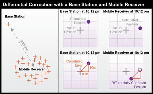
The base station calculates the correction needed to eliminate the error in the position calculated at that moment from GPS signals. The correction is later applied to the position calculated by the mobile receiver at the same instant. The corrected position is not perfectly accurate because the kinds and magnitudes of errors affecting the two receivers are not identical, and because of the low frequency of the GPS timing code.

For differential correction to work, fixes recorded by the mobile receiver must be synchronized with fixes recorded by the base station (or stations). You can provide your own base station, or use correction signals produced from reference stations maintained by the U.S. Federal Aviation Administration, the U.S. Coast Guard, or other public agencies or private subscription services. Given the necessary equipment and available signals, synchronization can take place immediately ("real-time") or after the fact ("post-processing"). First let's consider real-time differential.

5.4.1 Real-time Differential Correction

WAAS-enabled receivers are an inexpensive example of real-time differential correction. "WAAS" stands for Wide Area Augmentation System [6], a collection of about 25 base stations set up to improve GPS positioning at U.S. airport runways to the point that GPS can be used to help land airplanes (U.S. Federal Aviation Administration, 2007c). WAAS base stations transmit their measurements to a master station, where corrections are calculated and then uplinked to two geosynchronous satellites (19 are planned). The WAAS satellite then broadcasts differentially-corrected signals at the same frequency as GPS signals. WAAS signals compensate for positioning errors measured at WAAS base stations, as well as clock error corrections and regional estimates of upper-atmosphere errors (Yeazel, 2003). The WAAS network was designed to provide approximately 7-meter accuracy uniformly throughout its U.S. service area when WAAS-enabled receivers are used.

DGPS: The U.S. Coast Guard has developed a similar system, called the Differential Global Positioning Service [7]. The DGPS network includes some 80 broadcast sites, each of which includes a survey-grade base station and a "radio beacon" transmitter that broadcasts correction signals at 285-325 kHz (just below the AM radio band). DGPS-capable GPS receivers include a connection to a radio receiver that can tune into one or more selected "beacons." Designed for navigation at sea near U.S. coasts, DGPS provides accuracies no worse than 10 meters.

Kinematic Positioning: Survey-grade real-time differential correction can be achieved using a technique called real-time kinematic (RTK) GPS. RTK uses carrier-phase tracking of GPS signals measured by a reference and a remote receiver to generate accuracies of 1 part in 100,000 to 1 part in 750,000 (in practice, this means within centimeters) with relatively brief observations of only one to two minutes each.

5.4.2 Post-processed Differential Correction

For applications that require accuracies of 1 part in 1,000,000 or higher, including control surveys and measurements of movements of the Earth's tectonic plates, static positioning is required (Van Sickle, 2001). In static GPS positioning, two or more receivers measure their positions from fixed locations over periods of 30 minutes to two hours. The receivers may be positioned up to 300 km apart. Only dual frequency, carrier phase differential receivers capable of measuring the differences in time of arrival of the civilian GPS signal (L1) and the encrypted military signal (L2) are suitable for such high-accuracy static positioning.

CORS and OPUS: The U.S. National Geodetic Survey (NGS) maintains an Online Positioning User Service (OPUS) that enables surveyors to differentially-correct static GPS measurements acquired with a single dual frequency carrier phase differential receiver after they return from the field. Users upload measurements in a standard Receiver INdependent EXchange format (RINEX) to NGS computers, which perform differential corrections by referring to three base stations selected from a network of continuously operating reference stations (CORS). NGS oversees two CORS networks; one consisting of its 600 base stations of its own, another is a cooperative of public and private agencies that agree to share their base station data and to maintain base stations to NGS specifications.

Ease, accuracy, and worldwide availability have made ‘GPS’ a household term. Yet, none of the power or capabilities of GPS would have been possible without traditional surveyors paving the way. The techniques and tools of conventional surveying are still in use and, as you will see, are based on the very same concepts that underpin even the most advanced satellite-based positioning.

Geographic positions are specified relative to a fixed reference. Positions on the globe, for instance, may be specified in terms of angles relative to the center of the Earth, the equator, and the prime meridian.

Land surveyors measure horizontal positions in geographic or plane coordinate systems relative to previously surveyed positions called control points, most of which are indicated physically in the world with a metal “benchmark” that fixes the location and, as shown here, may also indicate elevation about mean sea level (Figure 5.10). In 1988 NGS established four orders of control point accuracy, ranging in maximum base error from 3mm to 5cm. In the U.S., the National Geodetic Survey (NGS) maintains a National Spatial Reference System (NSRS) that consists of approximately 300,000 horizontal and 600,000 vertical control stations (Doyle,1994).

Doyle (1994) points out that horizontal and vertical reference systems coincide by less than ten percent. This is because:

....horizontal stations were often located on high mountains or hilltops to decrease the need to construct observation towers usually required to provide line-of-sight for triangulation, traverse and trilateration measurements. Vertical control points however, were established by the technique of spirit leveling which is more suited to being conducted along gradual slopes such as roads and railways that seldom scale mountain tops. (Doyle, 2002, p. 1)

You might wonder how a control network gets started. If positions are measured relative to other positions, what is the first position measured relative to? The answer is: the stars. Before reliable timepieces were available, astronomers were able to determine longitude only by careful observation of recurring celestial events, such as eclipses of the moons of Jupiter. Nowadays, geodesists produce extremely precise positional data by analyzing radio waves emitted by distant stars. Once a control network is established, however, surveyors produce positions using instruments that measure angles and distances between locations on the Earth's surface.

Figure 5.10: Benchmark used to mark a vertical control point.

Credit: Thompson, 1988.

5.5.1 Measuring Angles and Distances

You probably have seen surveyors working outside, e.g., when highways are being realigned or new housing developments are being constructed. Often one surveyor operates equipment on a tripod while another holds up a rod some distance away.  What the surveyors and their equipment are doing is carefully measuring angles and distances, from which positions and elevation can be calculated. We will briefly discuss this equipment and their methodology. Let us first take a look at angles and how they apply to surveying.

Although a standard compass can give you a rough estimate of angles, the Earth’s magnetic field is not constant and the magnetic poles, which slowly move over time, do not perfectly align with the planet’s axis of rotation; as a result of the latter, true (geographic) north and magnetic north are different. Moreover, some rocks can become magnetized and introduce subtle local anomalies when using compass. For these reasons, land surveyors rely on transits (or their more modern equivalents, called theodolites) to measure angles. A transit (Figure 5.11) consists of a telescope for sighting distant target objects, two measurement wheels that work like protractors for reading horizontal and vertical angles, and bubble levels to ensure that the angles are true. A theodolite is essentially the same instrument, except that it is somewhat more complex and capable of higher precision. In modern theodolites, some mechanical parts are replaced with electronics.

Figure 5.11: A traditional transit once used by surveyors.

Credit: Raisz, 1948, Used by permission.

When surveyors measure angles, the resultant calculations are typically reported as either azimuths or bearings, as seen in Figure 5.12. A bearing is an angle less than 90° within a quadrant defined by the cardinal directions. An azimuth is an angle between 0° and 360° measured clockwise from North. "South 45° East" and "135°" are the same direction expressed as a bearing and as an azimuth.

Figure 5.12: Azimuths and Bearings. Note that an azimuth of 360° is the same as 0°.

Credit: Department of Geography, The Pennsylvania State University.

5.5.2 Measuring Distances

To measure distances, land surveyors once used 100-foot long metal tapes that are graduated in hundredths of a foot. An example of this technique is shown in Figure 5.13. Distances along slopes were measured in short horizontal segments. Skilled surveyors could achieve accuracies of up to one part in 10,000 (1 centimeter error for every 100 meters distance). Sources of error included flaws in the tape itself, such as kinks; variations in tape length due to extremes in temperature; and human errors such as inconsistent pull, allowing the tape to stray from the horizontal plane, and incorrect readings.

Figure 5.13: Surveying team measuring a baseline distance with a metal (Invar) tape.

Credit: Hodgson, 1916.

Since the 1980s, electronic distance measurement(EDM) devices have allowed surveyors to measure distances more accurately and more efficiently than they can with tapes. To measure the horizontal distance between two points, one surveyor uses an EDM instrument to shoot an energy wave toward a reflector held by the second surveyor. The EDM records the elapsed time between the wave's emission and its return from the reflector. It then calculates distance as a function of the elapsed time (not unlike what we’ve learned about GPS!). Typical short-range EDMs can be used to measure distances as great as 5 kilometers at accuracies up to one part in 20,000, twice as accurate as taping.

Instruments called total stations (Figure 5.14) combine electronic distance measurement and the angle measuring capabilities of theodolites in one unit. Next we consider how these instruments are used to measure horizontal positions in relation to established control networks.

Figure 5.14: A modern total station.

Credit: Łukasz Fus.

5.5.3 Combining Angles and Distances to Determine Positions

Surveyors have developed distinct methods, based on separate control networks, for measuring horizontal and vertical positions. In this context, a horizontal position is the location of a point relative to two axes: the equator and the prime meridian on the globe, or to the x and y axes in a plane coordinate system.

We will now introduce two techniques that surveyors use to create and extend control networks (triangulation and trilateration) and two other techniques used to measure positions relative to control points (open and closed traverses).

Surveyors typically measure positions in series. Starting at control points, they measure angles and distances to new locations, and use trigonometry to calculate positions in a plane coordinate system. Measuring a series of positions in this way is known as "running a traverse." A traverse that begins and ends at different locations, in which at least one end point is initially unknown, is called an open traverse. A traverse that begins and ends at the same point, or at two different but known points, is called a closed traverse. "Closed" here does not mean geometrically closed (as in a polygon) but mathematically closed (defined as: of or relating to an interval containing both its endpoints). By "closing" a route between one known location and another known location, the surveyor can determine errors in the traverse.

Measurement errors in a closed traverse that connects at the point where it started can be quantified by summing the interior angles of the polygon formed by the traverse. The accuracy of a single angle measurement cannot be known, but since the sum of the interior angles of a polygon is always (n-2) × 180, it's possible to evaluate the traverse as a whole, and to distribute the accumulated errors among all the interior angles. Errors produced in an open traverse, one that does not end where it started, cannot be assessed or corrected. The only way to assess the accuracy of an open traverse is to measure distances and angles repeatedly, forward and backward, and to average the results of calculations. Because repeated measurements are costly, other surveying techniques that enable surveyors to calculate and account for measurement error are preferred over open traverses for most applications.

5.5.4 Triangulation

Closed traverses yield adequate accuracy for property boundary surveys, provided that an established control point is nearby. Surveyors conduct control surveys to extend and add point density to horizontal control networks. Before survey-grade satellite positioning was available, the most common technique for conducting control surveys was triangulation (Figure 5.16).

Figure 5.15: Establishing new control points by triangulation from an existing control point (A).

Credit: Department of Geography, The Pennsylvania State University. Adapted from DiBiase's original text (1997).

1. Using a total station equipped with an electronic distance measurement device, the control survey team commences by measuring the azimuth alpha, and the baseline distance AB.
2. These two measurements enable the survey team to calculate position B as in an open traverse.
3. The surveyors next measure the interior angles CAB, ABC, and BCA at point A, B, and C. Knowing the interior angles and the baseline length, the trigonometric "law of sines" can then be used to calculate the lengths of any other side. Knowing these dimensions, surveyors can fix the position of point C.
4. Having measured three interior angles and the length of one side of triangle ABC, the control survey team can calculate the length of side BC. This calculated length then serves as a baseline for triangle BDC. Triangulation is thus used to extend control networks, point by point and triangle by triangle.

5.5.5 Trilateration

An alternative to triangulation is trilateration, which uses distances alone to determine positions. By eschewing angle measurements, trilateration is easier to perform, requires fewer tools, and is therefore less expensive. Having read this chapter so far, you have already been introduced to a practical application of trilateration, since it is the technique behind satellite ranging used in GPS.

You have seen an example of trilateration in Figure 5.8 in the form of 3-dimensional spheres extending from orbiting satellites. Demo 1 below steps through this process in two dimensions.

Once a distance from a control point is established, a person can calculate a distance by open traverse, or rely on a known distance if one exists. A single control point and known distance confines the possible locations of an unknown point to the edge of the circle surrounding the control point at that distance; there are infinitively many possibilities along this circle for the unknown location. The addition of a second control point introduces another circle with a radius equal to its distance from the unknown point. With two control points and distance circles, the number of possible points for the unknown location is reduced to exactly two. A third and final control point can be used to identify which of the remaining possibilities is the true location.

Trilateration is noticeably simpler than triangulation and is a very valuable skill to possess. Even with very rough estimates, one can determine a general location with reasonable success.

Positions are a fundamental element of geographic data. Sets of positions form features, as the letters on this page form words. Positions are produced by acts of measurement, which are susceptible to human, environmental, and instrument errors. Measurement errors cannot be eliminated, but systematic errors can be estimated and compensated for.

This chapter has introduced some of the technologies and techniques used in the acquisition of locational data. You have learned how a variety of location-enabled devices make use of signals from orbiting satellites and how satellite ranging is similar to more traditional surveying methods used on the ground. You have also learned how satellite technologies and surveying instruments can be used in conjunction to correct errors and generate data with higher accuracy.

Now that you know how GPS works, you can start putting it to work. The short list below includes some activities you can do with GPS and the techniques you’ve learned in this chapter:

1. Go geocaching! Visit GeoCaching.com [8] or OpenCaching.com [9] to get started.
2. Turn on your GPS and create shapes by tracking your path through town: Bostovalentinography [10]
3. Do you like to jog? Track, time, and trace your runs: Try MapMyRun.com [11] or TrainingPeaks.com [12]
4. Find and catalogue confluences. You’re never farther than 49 miles from a confluence, or location where both latitude and longitude are whole numbers. Go find one! Confluence.org [13]
5. Measure your yard, record your favorite fishing spot, or enhance your golf game by knowing just how far the pin is. The possibilities are endless.

Accuracy: How close or far a measurement is from the true or accepted value. Close measurements are more accurate than those that a further from the real value.

Additive Correction: A singular amount that is added to or subtracted from a series of measurements as a means to reduce systematic error.

Azimuth: Measurements of direction in terms of degrees, ranging from 0° to 360°.

Bearing: An angle less than 90° within a quadrant defined by the cardinal directions.

Closed Traverse: A measurement of distance between a single point and an unknown point that begins and ends at the same location.

Control Segment: The segment of the Global Positioning System that is comprised of ground stations that monitor and analyze satellite orbits and send corrections as needed.

Data Quality: The fitness of data for their intended use.

DGPS: Differential Global Positioning Service. DGPS offers enhanced locational measurements through the use of radio beacons that provide corrections.

Differential Correction: The use of control station to acquire a differential calculation which is then sent to local receivers to increase the accuracy of their measurements.

Dilution Of Precision (DOP): A factor that multiplies the uncertainty associated with User Equivalent Range Errors, based on the current configuration of viewable satellites. A DOP of 1 represents an ideal scenario, though real-world experiences seldom notice a DOP less than 2.

Environmental Characteristics: Variations in temperature, gravity, and magnetic declination that contribute to measurement errors.

GPS: The Global Positioning System.

Human Errors: Mistakes, improper use of equipment, and poor judgment that leads to measurement errors.

Instrument Errors: Errors that result from limitations related to the finite resolution of measuring equipment and its application in an infinite, continuous space.

Multipath Error: GPS errors that result from poor view of orbiting satellites, which are affected by buildings, valleys, the atmosphere, and other elements that can block, reflect, or refract GPS signals.

Open Traverse: A measurement of distance between a single point and an unknown point that begins and ends at different locations.

Precision: How reliably similar measurements can be taken with respect to variation and resolution.

Proportional Correction: Identifying a trend and applying the proper equation to adjust measurements in an attempt to correct inconsistent systematic errors.

Random Errors: Errors that do not follow a trend and are off by various amounts with no discernable pattern.

Resolution: The smallest measurement unit that can be detected or represented. High resolution refers to smaller units while low resolution refers to larger, and therefore fewer, units of measurement in the same space.

Satellite Ranging: Calculating distances from observable satellites based on their internal clocks and the amount of time taken for a signal to reach a corresponding receiver.

Space Segment: The segment of the Global Positioning System that is composed of a constellation of satellites following a precisely defined array of orbital planes.

Systemic Errors: Errors in measurement that follow a systematic and calculable trend.

Theodolites: Electronic equipment used in surveying for precise and accurate measuring of angles.

Total Station: A surveying instrument that is capable of electronic distance ranging as well as the angle measuring abilities of theodolites.

Triangulation: A trigonometric process of determining the position of unknown points based on the angles and distances calculated from a known point and a determined baseline.

Trilateration: The use of distances from known points to determine the position of an unknown point. At least three known locations are required for two-dimensional trilateration, while four known distances allows 3-dimensions (horizontal plus elevation).

User Segment: The segment of the Global Positioning System that is made up of devices that can receive satellite signals and the humans who operate these devices.

Wide Area Augmentation System (WAAS): The system of ground reference stations and geostationary satellites that enable the calculation and broadcast of corrected GPS signals.