Lessons
Lesson 1: Introduction to GIS modeling and Python
The links below provide an outline of the material for this lesson. Be sure to carefully read through the entire lesson before returning to Canvas to submit your assignments.
Lesson 1 Overview
Welcome to Geography 485. Over the next ten weeks, you'll work through four lessons and a final project dealing with ArcGIS automation in Python. Each lesson will contain readings, examples, and projects. Since the lessons are two weeks long, you should plan between 20 - 30 hours of work to complete them, although this number may vary depending on your prior programming experience. See the Course Schedule section of this syllabus, below, for a schedule of the lessons and course projects.
As with GEOG 483 and GEOG 484, the lessons in this course are project-based with key concepts embedded within. However, because of the nature of computer programming, there is no way this course can follow the step-by-step instructional design of the previous courses. You will probably find the course to be more challenging than our courses on GIS fundamentals. For that reason, it is more important than ever that you stay on schedule and take advantage of the course message boards and private email. It's quite likely that you will get stuck somewhere during the course, so before getting hopelessly frustrated, please seek help from me or your classmates!
I hope that by now that you have reviewed our Orientation and Syllabus for an important course site overview. Before we begin our first project, let me share some important information about the textbook and a related Esri course.
Textbook and Readings
The textbook for this course is Python Scripting for ArcGIS Pro by Paul A. Zandbergen. As you read through Zandbergen's book, you'll see material that closely parallels what is in the Geog 485 lessons. This isn't necessarily a bad thing; when you are learning a subject like programming, it can be helpful to have the same concept explained from two angles.
My advice about the readings is this: Read the material on the Geog 485 lesson pages first. If you feel like you have a good understanding from the lesson pages, you can skim through some of the more lengthy Zandbergen readings. If you struggled with understanding the lesson pages, you should pay close attention to the Zandbergen readings and try some of the related code snippets and exercises. I suggest you plan about 1 - 2 hours per week of reading if you are going to study the chapters in detail.
In all cases, you should get a copy of the textbook because it is a relevant and helpful reference.
Note:
The Zandbergen textbook is up to the 3rd Edition as of Summer 2024. The free copy of the book available through the PSU library is the 2nd Edition. Differences between the two editions are relatively minor and you may assume that the section numbers referenced here in the lessons are applicable to both editions unless otherwise noted.
You may see that in Esri's documentation, shapefiles are also referred to as "feature classes." When you see the term "feature class," consider it to mean a vector dataset that can be used in ArcGIS.
Another type of standalone dataset dating back to the early days of ArcGIS is the ArcInfo coverage. Like the shapefile, the coverage consists of several files that work together. Coverages are definitely an endangered species, but you might encounter them if your organization used ArcInfo Workstation in the past.
Esri Virtual Campus Course Python for Everyone
There is a free Esri Virtual Campus course, Python for Everyone [1], that introduces a lot of the same things you'll learn this term in Geog 485. Python for Everyone consists of a series of short videos and exercises, some of which might help toward the projects. If you want to get a head start, or you want some reinforcement of what we're learning from a different point of view, it would be worth your time to complete that Virtual Campus course.
All you need in order to access the course is an Esri Global Account, which you can create for free. You do not need to obtain an access code from Penn State.
The course moves through ideas very quickly and covers a range of concepts that we'll spend 10 weeks studying in depth, so don't worry if you don't understand it all immediately or if it seems overwhelming. You might find it helpful to quickly review the course again near the end of Geog 485 to review what you've learned.
Questions?
If you have any questions now or at any point during this week, please feel free to post them to the Lesson 1 Discussion Forum. (To access the forums, return to Canvas via the Canvas link. Once in Canvas, you can navigate to the Modules tab, and then scroll to the Lesson 1 Discussion Forum.) While you are there, feel free to post your own responses if you are able to help a classmate.
Now, let's begin Lesson 1.
Lesson 1 Checklist
This lesson is two weeks in length. (See the Calendar in Canvas for specific due dates.) To finish this lesson, you must complete the activities listed below. You may find it useful to print this page so that you can follow along with the directions.
- Download the Lesson 1 data [2] and extract it to C:\PSU\Geog485\Lesson1 or a similar path that is easy to remember.
- Work through the online sections of Lesson 1.
- Read the assigned pages from the Zandbergen textbook. In the online lesson pages, I have inserted instructions on the sections to read from Zandbergen when it is most appropriate to read them.
- Complete Project 1, Part I and submit the deliverables to the course drop box in Canvas.
- Complete Project 1, Part II and submit the deliverables to the course drop box in Canvas.
- Complete the Lesson 1 Quiz in Canvas.
Do items 1 - 3 (including any of the practice exercises you want to attempt) during the first week of the lesson. You will need the second week to concentrate on the project and quiz.
Lesson objectives
By the end of this lesson, you should:
- be able to create automated workflows in ArcGIS Pro ModelBuilder;
- be familiar with the PyScripter development environment;
- know some of Python’s most important basic data types and how to use variables in Python scripts;
- be familiar with the basic concepts of object oriented programming (e.g. classes & inheritance);
- be able to use arcpy tool functions to achieve basic spatial analysis tasks; and
- know how to create a simple script tool and pass a parameter to a script.
1.1.1 The need for GIS automation
A geographic information system (GIS) can manipulate and analyze spatial datasets with the purpose of solving geographic problems. GIS analysts perform all kinds of operations on data to make it useful for solving a focused problem. This includes clipping, reprojecting, buffering, merging, mosaicking, extracting subsets of the data, and hundreds of other operations. In the ArcGIS software used in this course, these operations are known as geoprocessing and they are performed using tools.
Successful GIS analysis requires selecting the most appropriate tools to operate on your data. ArcGIS uses a toolbox metaphor to organize its suite of tools. You pick the tools you need and run them in the proper order to make your finished product.
Suppose you’re responsible for selecting sites for a chain restaurant. You might use one tool to select land parcels along a major thoroughfare, another tool to select parcels no smaller than 0.25 acres, and other tools for other selection criteria. If this selection process were limited to a small area, it would probably make sense to perform the work manually.
However, let’s suppose you’re responsible for carrying out the same analysis for several areas around the country. Because this scenario involves running the same sequence of tools for several areas, it is one that lends itself well to automation. There are several major benefits to automating tasks like this:
- Automation makes work easier. Once you automate a process, you don't have to put in as much effort remembering which tools to use or the proper sequence in which they should be run.
- Automation makes work faster. A computer can open and execute tools in sequence much faster than you can accomplish the same task by pointing and clicking.
- Automation makes work more accurate. Any time you perform a manual task on a computer, there is a chance for error. The chance multiplies with the number and complexity of the steps in your analysis, as well as the fatigue incurred by repeating the task many times. In contrast, once an automated task is configured, a computer can be trusted to perform the same sequence of steps every time for a potentially endless number of cycles.
The ArcGIS platform provides several ways for users to automate their geoprocessing tasks. These options differ in the amount of skill required to produce the automated solution and in the range of scenarios that each can address. The text below touches briefly on these automation options, in order from requiring the least coding skill to the most.
The first option is to construct a model using ModelBuilder. ModelBuilder is an interactive program that allows the user to “chain” tools together, using the output of one tool as input in another. Perhaps the most attractive feature of ModelBuilder is that users can automate rather complex GIS workflows without the need for programming. You will learn how to use ModelBuilder early in this course.
Some automation tasks require greater flexibility than is offered by ModelBuilder, and for these scenarios it's recommended that you write short computer programs, or scripts. The bulk of this course is concerned with script writing.
A script typically executes some sequential procedure of steps. Within a script, you can run GIS tools individually or chain them together. You can insert conditional logic in your script to handle cases where different tools should be run depending on the output of the previous operation. You can also include iteration, or loops, in a script to repeat a single action as many times as needed to accomplish a task.
There are special scripting languages for writing scripts, including Python, JScript, and Perl. Often these languages have more basic syntax and are easier to learn than other languages such as C, Java, or Visual Basic.
Although ArcGIS supports various scripting languages for working with its tools, Esri emphasizes Python in its documentation and includes Python with the ArcGIS Desktop and Pro installations. In this course, we’ll be working strictly with Python for this reason, as well as the fact that Python can be used for many other file and data manipulation tasks outside of ArcGIS. You’ll learn the basics of the Python language, how to write a script, and how to manipulate and analyze GIS data using scripts. Finally, you’ll apply your new Python knowledge to a final project, where you write a script of your choosing that you may be able to apply directly to your work.
A more recently developed automation option available on the ArcGIS platform is the ArcGIS API (Application Programming Interface) for Python. This is an environment in which Python scripting is better integrated with Esri's cloud- and server-based technologies (ArcGIS Online, Portal for ArcGIS, ArcGIS Enterprise). Code written to interact with the Python API is often written in a "notebook" environment, such as Jupyter Notebook. In a notebook environment, code can be executed in a stepwise fashion, with intermediate results displayed in between the Python statements. The use of the Python API in a Jupyter Notebook environment is a topic in our Advanced Python class, GEOG 489.
For geoprocessing tasks that require support for user interaction with the map or other UI elements, the ArcGIS Pro SDK (Software Development Kit) offers the ability to add custom tools to the Pro interface. The Pro SDK requires programming in the .NET framework using a .NET language such as Visual Basic .NET or C#. Working with this SDK's object model provides greater flexibility in terms of what can be built, as compared to writing Python scripts around their geoprocessing framework. The tradeoff is a higher level of complexity involved in the coding.
Finally, developers who want to create their own custom GIS applications, typically focused on delivering much narrower functionality than the one-size-fits-all ArcGIS Pro, can develop apps using the ArcGIS Maps SDKs (previously called Runtime SDKs). The Maps SDKs make it possible to author apps for Windows, Mac, or Linux desktop machines, as well as for iOS and Android mobile devices, again involving a greater level of effort than your typical Python geoprocessing script. In the past, there was a native version for MacOS but that has been retired. Instead, programmers can use the Maps SDK for Java version to develop for MacOS.
This first lesson will introduce you to concepts in both model building and script writing. We’ll start by just getting familiar with how tools run in ArcGIS and how you can use those tools in the ModelBuilder interface. Then, we’ll cover some of the basics of Python and see how the tools can be run within scripts.
1.2.1 Exploring the toolbox
The ArcGIS software that you use in this course contains hundreds of tools that you can use to manipulate and analyze GIS data. Back before ArcGIS had a graphical user interface (GUI), people would access these tools by typing commands. Nowadays, you can point and click your way through a whole hierarchy of toolboxes using the Catalog window in ArcGIS Pro.
Although you may have seen them before, let’s take a quick look at the toolboxes:
- Open a new or existing project in ArcGIS Pro.
- If the Geoprocessing pane isn't visible, click the Analysis tab, then click Tools.
- In the Geoprocessing pane, click the Toolboxes tab heading. Notice that the tools are organized into toolboxes and toolsets. For example, the IDW and Spline tools can be found in the Interpolation toolset within the Spatial Analyst toolbox. Sometimes it’s faster to use the Find Tools box at the top of the Geoprocessing tab to find the tool you need instead of browsing this tree.
-
Let’s examine a tool. Expand Analysis Tools > Proximity > Buffer, and double-click the Buffer tool to open it.
You've probably seen this tool in past courses, but this time, really pay attention to the components that make up the user interface. Specifically, you’re looking at a dialog with many fields. Each geoprocessing tool has required inputs and outputs. Those are indicated by the red asterisks. They represent the minimum amount of information you need to supply in order to run a tool. For the Buffer tool, you’re required to supply an input features location (the features that will be buffered) and a buffer distance. You’re also required to indicate an output feature class location (for the new buffered features).
Many tools also have optional parameters. You can modify these if you want, but if you don’t supply them, the tool will still run using default values. For the Buffer tool, optional parameters are the Side Type, End Type, Method, and Dissolve Type. Optional parameters are typically specified after required parameters.
-
Hover your mouse over any of the tool parameters. You should see a blue "info" icon to the left of the parameter. Moving your mouse over that icon will show a brief description of the parameter in a pop-out window.
If you’re not sure what a parameter means, this is a good way to learn. For example, viewing the pop-out documentation for the End Type parameter will show you an explanation of what this parameter means and list the two options: Round and Flat.
If you need even more help, each tool is more expansively documented in the ArcGIS Pro web-based help system. You can access a tool's documentation in this system by clicking on the blue ? icon in the upper-right of the tool dialog, which will open the help page in your default web browser.
- Open the web-based help page for the Buffer tool. As mentioned, the help page will provide extensive documentation of the tool's usage. In the upper right of the help page, you should see a list of links that are shortcuts to various sections of the tool's documentation.
- Click the Parameters link to jump to that section. There you should find that the information is divided between two tabs (Dialog and Python), with the Dialog tab displayed by default. The Dialog tab focuses on providing help to those who are executing the tool through the ArcGIS Pro GUI, while the Python tab focuses on providing help to those who are invoking it through a Python script.
- Click on the Python tab, since that's our focus in this class. You should see the name, a description, and the data type associated with each of the tool's parameters. That information is certainly helpful, but often even more helpful is the Code sample section that appears below the parameter list. Every tool's help page has these programming examples showing ways to run the tool from within a script, and they will be extremely valuable to you as you complete the assignments in this course.
1.2.2 Environments for accessing tools
You can access ArcGIS geoprocessing tools in several different ways:
- Sometimes you just need to run a tool once, or you want to experiment with a tool and its parameters. In this case, you can open the tool directly from the Geoprocessing pane and use the tool’s graphical user interface (GUI, pronounced gooey) to fill in the parameters.
- ModelBuilder is also a GUI application where you can set up tools to run in a given sequence, using the output of one tool as input to another tool.
- If you’re familiar with the tool and want to use it quickly in Pro, you may prefer the Python window approach. You type the tool name and required parameters into a command window. You can use this window to run several tools in a row and declare variables, effectively doing simple scripting.
- If you want to run the tool automatically, repeatedly, or as part of a greater logical sequence of tools, you can run it from a script. Running a tool from a script is the most powerful and flexible option.
We’ll start with the simplest of these cases, running a tool from its GUI, and work our way up to scripting.
1.2.3 Running a tool from its GUI
Let’s start by opening a tool from the Catalog pane and running it using its graphical user interface (GUI).
- If, by chance, you still have the Buffer tool open from the previous section, close it for now so you can add some data.
- Create a folder on your machine at C:\PSU\Geog485. If you use a different path, be sure to substitute your path in the following examples.
- Download the Lesson 1 data [2] and extract Lesson1.zip into your new folder so that the data is under the path C:\PSU\Geog485\Lesson1. This folder contains a variety of datasets you will use throughout the lesson.
- Open a new project in Pro if you don't have one open already.
- Click the Add Data button
 and browse to the data you just extracted. Add the us_boundaries and us_cities shapefiles.
 - Open the Geoprocessing pane if necessary and browse to the Buffer tool as you did in the previous section.
- Double-click the Buffer tool to open it.
-
Examine the first required parameter: Input Features. Click the Browse button
 and browse to the path of your cities dataset C:\PSU\Geog485\Lesson1\us_cities.shp. Notice that once you do this, a name is automatically supplied for the Output Feature Class (and the output path is the same as the input features). The software does this for your convenience only, and you can change the name/path if you want.
A more convenient way to supply the Input Features is to just select the cities map layer from the dropdown menu. This dropdown automatically contains all the layers in your map. However, in this example, we browsed to the path of the data because it’s conceptually similar to how we’ll provide the paths in the command line and scripting environments.
- Now you need to supply the Distance parameter for the buffer. For this run of the tool, set a Linear unit of 5 miles. When we run the tool from the other environments, we’ll make the buffer distance slightly larger, so we know that we got distinct outputs.
- The rest of the parameters are optional. The Side Type parameter applies only to lines and polygons, so it is not even available for setting in the GUI environment when working with city points. However, change the Dissolve Type to Dissolve all output features into a single feature. This combines overlapping buffers into a single polygon.
- Leave the Method set to Planar. We're not going to take the earth's curvature into account for this simple example.
- Click Run to execute the tool.
- The tool should take just a few seconds to complete. Examine the output that appears on the map, and do a “sanity check” to make sure that buffers appear around the cities, and they appear to be about 5 miles in radius. You may need to zoom in to a single state in order to see the buffers.
- Click on Pro's Analysis tab, then on History (in the Geoprocessing button group). This will open the History tab in Pro's Catalog pane, which lists messages about successes or failures of all recent tools that you've run.
-
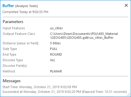
Hover over the Buffer tool entry in this list to see a pop-out window. This window lists the tool parameters, the time of completion, and any problems that occurred when running the tool (see Figure 1.1). These messages can be a big help later when you troubleshoot your Python scripts. The text of these messages is available whether you run the tool from the GUI, from the Python window in Pro, or from scripts.
1.2.4 Modeling with tools
When you work with geoprocessing, you’ll frequently want to use the output of one tool as the input into another tool. For example, suppose you want to find all fire hydrants within 200 meters of a building. You would first buffer the building, then use the output buffer as a spatial constraint for selecting fire hydrants. The output from the Buffer tool would be used as an input to the Select by Location tool.
A set of tools chained together in this way is called a model. Models can be simple, consisting of just a few tools, or complex, consisting of many tools and parameters and occasionally some iterative logic. Whether big or small, the benefit of a model is that it solves a unique geographic problem that cannot be addressed by one of the “out-of-the-box” tools.
In ArcGIS, modeling can be done either through the ModelBuilder graphical user interface (GUI) or through code, using Python. To keep our terms clear, we’ll refer to anything built in ModelBuilder as a “model” and anything built through Python as a “script.” However, it’s important to remember that both things are doing modeling.
1.3.1 Why learn ModelBuilder?
ModelBuilder is Esri’s graphical interface for making models. You can drag and drop tools from the Catalog pane into the model and “connect” them, specifying the order in which they should run.
Although this is primarily a programming course, we’ll spend some time in ModelBuilder during the first lesson for two reasons:
- ModelBuilder is a nice environment for exploring the ArcGIS tools, learning how tool inputs and outputs are used, and visually understanding how GIS modeling works. When you begin using Python, you will not have the same visual assistance to see how the tools you’re using are connected, but you may still want to draw your model on a whiteboard in a similar fashion to what you saw in ModelBuilder.
- ModelBuilder can frequently reduce the amount of Python coding that you need to do. If your GIS problem does not require advanced conditional and iterative logic, you may be able to get your work done in ModelBuilder without writing a script. ModelBuilder also allows you to export any model to Python code, so if you get stuck implementing some tools within a script, it may be helpful to make a simple working model in ModelBuilder, then export it to Python to see how ArcGIS would construct the code. (Exporting a complex model is not recommended for beginners due to the verbose amount of code that ModelBuilder tends to create when exporting Python).
1.3.2 Opening and exploring ModelBuilder
Let’s get some practice with ModelBuilder to solve a real scenario. Suppose you are working on a site selection problem where you need to select all areas that fall within 10 miles of a major highway and 10 miles of a major city. The selected area cannot lie in the ocean or outside the United States. Solving the problem requires that you make buffers around both the roads and the cities, intersect the buffers, then clip to the US outline. Instead of manually opening the Buffer tool twice, followed by the Intersect tool, then the Clip tool, you can set this up in ModelBuilder to run as one process.
- Create a new Pro project called Lesson1Practice in the C:\PSU\Geog485\Lesson1 folder.
- Add the us_cities, us_roads, and us_boundaries shapefiles from the Lesson 1 data folder that you configured previously in this lesson to a new map.
- In the Catalog pane, right-click your Lesson1Practice toolbox and click New > Model. You’ll see ModelBuilder appear in the middle of the Pro window.
- Under the ModelBuilder tab, click the Properties button.
- For the Name, type SuitableLand and for the Label, type Find Suitable Land. The label is what everyone will see when they open your tool from the Catalog. That’s why it can contain spaces. The name is what people will use if they ever run your model from Python. That’s why it cannot contain spaces.
-
Click OK to dismiss the model Properties dialog.
You now have a blank canvas on which you can drag and drop the tools. When creating a model (and when writing Python scripts), it’s best to break your problem into manageable pieces. The simple site selection problem here can be thought of as four steps:
- Buffer the cities
- Buffer the roads
- Intersect the buffers
- Clip to the US boundary
Let’s tackle these items one at a time, starting with buffering the cities.
- With ModelBuilder still open, go to the Catalog pane > Geoprocessing tab and browse to Analysis Tools > Proximity.
-
Click the Buffer tool and drag it onto the ModelBuilder canvas. You’ll see a gray rectangular box representing the buffer tool and a gray oval representing the output buffers. These are connected with a line, showing that the Buffer tool will always produce an output data set.
In ModelBuilder, tools are represented with boxes and variables are represented with ovals. Right now, the Buffer tool, at center, is gray because you have not yet supplied the required parameters. Once you do this, the tool and the variable will fill in with color.
- In your ModelBuilder window, double-click the Buffer box. The tool dialog here is the same as if you had opened the Buffer directly from the Catalog pane. This is where you can supply parameters for the tool.
- For Input Features, browse to the path of your us_cities shapefile on disk. The Output Feature Class will populate automatically.
- For Distance [value or field], enter 10 miles.
- For Dissolve Type, select Dissolve all output features..., then click OK to close the Buffer dialog. The model elements (tools and variables) should be filled in with color, and you should see a new element to the left of the tool representing the input cities feature class.
-
An important part of working with ModelBuilder is supplying clear labels for all the elements. This way, if you share your model, others can easily understand what will happen when it runs. Supplying clear labels also helps you remember what the model does, especially if you haven’t worked with the model for a while.
In ModelBuilder, right-click the us_cities.shp element (blue oval, at far left) and click Rename. Name this element "US Cities."
- Right-click the Buffer tool (yellow-orange box, at center) and click Rename. Name this “Buffer the cities.”
-
Right-click the buffer output element (green oval, at far right) and click Rename. Name this “Buffered cities.” Your model should look like this.
 Figure 1.2 The model's appearance following step 15, above.
 - Save your model (ModelBuilder tab > Save). This is the kind of activity where you want to save often.
-
Practice what you just learned by adding another Buffer tool to your model. This time, configure the tool so that it buffers the us_roads shapefile by 10 miles. Remember to set the Dissolve type to Dissolve all output features... and to add meaningful labels. Your model should now look like this.
 Figure 1.3 The model's appearance following step 17, above.
 - The next task is to intersect the buffers. In the Catalog pane's list of toolboxes, browse to Analysis Tools > Overlay and drag the Intersect tool onto your model. Position it to the right of your existing Buffer tools.
- Here’s the pivotal moment when you chain the tools together, setting the outputs of your Buffer tools as the inputs of the Intersect tool. Click the Buffered cities element and drag over to the Intersect element. If you see a small menu appear, click Input Features to denote that the buffered cities will act as inputs to the Intersect tool. An arrow will now point from the Buffered cities element to the Intersect element.
- Use the same process to connect the Buffered roads to the Intersect element. Again, if prompted, click Input Features.
-
Rename the output of the Intersect operation "Intersected buffers." If the text runs onto multiple lines, you can click and drag the edges of the element to resize it. You can also rearrange the elements on the page however you like. Because models can get large, ModelBuilder contains several navigation buttons for zooming in and zooming to the full extent of the model in the View button group on the ribbon. Your model should now look like this:
 Figure 1.4 The model's appearance following step 21, above.
 - The final step is to clip the intersected buffers to the outline of the United States. This prevents any of the selected area from falling outside the country or in the ocean. In the Catalog pane, browse to Analysis Tools > Extract and drag the Clip tool into ModelBuilder. Position this tool to the right of your existing tools.
- As you did above, set the Intersected buffers as an input to the Clip tool, choosing Input Features when prompted. Notice that even when you do this, the Clip tool is not ready to run (it’s still shown as a gray rectangle, located at right). You need to supply the clip features, which is the shape to which the buffers will be clipped.
- In ModelBuilder (not in the Catalog pane), double-click the Clip tool. Set the Clip Features by browsing to the path of us_boundaries.shp, then click OK to dismiss the dialog. You’ll notice that a blue oval appeared, representing the Clip Features (US Boundaries).
-
Set meaningful labels for the remaining tools as shown below. Below is an example of how you can label and arrange the model elements.
 Figure 1.5 The completed model with the clip tool included.
 - Double-click the final output element (named "Suitable land" in the image above) and set the path to C:\PSU\Geog485\Lesson1\suitable_land.shp. This is where you can expect your model output feature class to be written to disk.
- Right-click Suitable land and click Add to display.
- Save your model again.
- Test the model by clicking the Run button.
 You’ll see the by-now-familiar geoprocessing message window that will report any errors that may occur. ModelBuilder also gives you a visual cue of which tool is running by turning the tool red. (If the model crashes, try closing ModelBuilder and running the model by double-clicking it from the Catalog pane. You'll get a message that the model has no parameters. This is okay [and true, as you'll learn below]. Go ahead and run the model anyway.)
 -
When the model has finished running (it may take a while), examine the output on the map. Zoom into Washington state to verify that the has Clip worked on the coastal areas. The output should look similar to this.
 Figure 1.6 The model's output in ArcGIS Pro.
That’s it! You’ve just used ModelBuilder to chain together several tools and solve a GIS problem.
You can double-click this model anytime in the Catalog pane and run it just as you would a tool. If you do this, you’ll notice that the model has no parameters; you can’t change the buffer distance or input features. The truth is, our model is useful for solving this particular site-selection problem with these particular datasets, but it’s not very flexible. In the next section of the lesson, we’ll make this model more versatile by configuring some of the variables as input and output parameters.
1.3.3 Model parameters
Most tools, models, and scripts that you create with ArcGIS have parameters. Input parameters are values with which the tool (or model or script) starts its work, and output parameters represent what the tool gives you after its work is finished.
A tool, model, or script without parameters is only good in one scenario. Consider the model you just built that used the Buffer, Intersect, and Clip tools. This model was hard-coded to use the us_cities, us_roads, and us_boundaries shapefiles and output a shapefile called suitable_land. In other words, if you wanted to run the model with other datasets, you would have to open ModelBuilder, double-click each element (US Cities, US Roads, US Boundaries, and Suitable land), and change the paths that were written directly into the model. You would have to follow a similar process if you wanted to change the buffer distances, too, since those were hard-coded to 10 miles.
Let’s modify that model to use some parameters, so that you can easily run it with different datasets and buffer distances.
- If it's not open already, open the project C:\PSU\Geog485\Lesson1\Lesson1Practice.aprx in ArcGIS Pro.
- In the Catalog window, find the model you created earlier in the lesson, which should be under Toolboxes > Lesson1Practice.atbx > Find Suitable Land.
- Right-click the model Find Suitable Land and click Copy. Now, right-click the Lesson1Practice toolbox and click Paste. This creates a new copy of your model that you can work with to create model parameters. Using a copy of the model like this allows you to easily start over if you make a mistake.
- Rename the copy of your model Find Suitable Land With Parameters or something similar.
- In your Lesson 1 toolbox, right-click Find Suitable Land With Parameters and click Edit. You'll see the model appear in ModelBuilder.
- Right-click the element US Cities (should be a blue oval) and click Parameter. This means that whoever runs the model must specify the cities dataset to use before the model can run.
- You need a more general name for this parameter now, so right-click the US Cities element and click Rename. Change the name to just "Cities."
-
Even though you "parameterized" the cities, your model still defaults to using the C:\PSU\Geog485\Lesson1\us_cities.shp dataset. This isn't going to make much sense if you share your model or toolbox with other people because they may not have the same us_cities shapefile, and even if they do, it probably won't be sitting at the same path on their machines.
To remove the default dataset, double-click the Cities element and delete the path, then click OK. Some of the elements in your model may turn gray. This signifies that a value has to be provided before the model can successfully run.
- Now you need to create a parameter for the distance of the buffer to be created around the cities. Right-click the element that you named "Buffer the cities" and click Create Variable > From Parameter > Distance [value or field].
- The previous step created a new element Distance [value or field]. Rename this element to "Cities buffer distance" and make it a model parameter. (Review the steps above if you're unsure about how to rename an element or make it a model parameter.) For this element, you can leave the default at 10 miles. Your model should look similar to this, although the title bar of your window may vary:
 Figure 1.7 The "Find Suitable Land With Parameters" model following Step 10, above, and showing two parameters.
Click link to expand for a text description of Figure 1.7. - Repeating what you learned above, rename the US Roads element to "Roads," make it a model parameter, and remove the default value.
- Repeating what you learned above, make a parameter for the Roads buffer distance. Leave the default at 10 miles.
- Repeating what you learned above, rename the US Boundaries element to Boundaries, make it a model parameter, and remove the default value. Your model should look like this (notice the five parameters indicated by "P"s):
 Figure 1.8 The "Find Suitable Land With Parameters" model following Step 13, above, and showing five parameters.
Click link to expand for a text description of Figure 1.8. - Save and close your model.
-
Double-click your model Lesson 1 > Find Suitable Land With Parameters and examine the tool dialog. It should look similar to this:
 Figure 1.9 The model interface, or tool dialog, for the model "Find Suitable Land With Parameters."
People who run this model will be able to browse to any cities, roads, and boundaries datasets, and will be able to control the buffer distance. The red asterisks indicate parameters that must be supplied with valid values before the model can run.
- Test your model by supplying the us_cities, us_roads, and us_boundaries shapefiles for the model parameters. If you like, you can try changing the buffer distance.
The above exercise demonstrated how you can expose values as parameters using ModelBuilder. You need to decide which values you want the user to be able to change and designate those as parameters. When you write Python scripts, you'll also need to identify and expose parameters in a similar way.
1.3.4 Advanced geoprocessing and ModelBuilder concepts
By now, you've had some practice with ModelBuilder, and you're about ready to get started with Python. This page of the lesson contains some optional advanced material that you can read about ModelBuilder. This is particularly helpful if you anticipate using ModelBuilder frequently in your employment. Some of the items are common to the ArcGIS geoprocessing framework, meaning that they also apply when writing Python scripts with ArcGIS.
Managing intermediate data
GIS analysis sometimes gets messy. Most of the tools that you run produce an output dataset, and when you chain many tools together, those datasets start piling up on disk. Esri has programmed ModelBuilder's default behavior such that when a model is run from a GUI interface, all datasets besides the final output -- referred to as intermediate data -- are automatically deleted. If, on the other hand, the model is run from ModelBuilder, intermediate datasets are left in their specified locations.
When running a model on another file system, specifying paths as we did above can be problematic, since the folder structure is not likely to be the same. This is where the concept of the scratch geodatabase (or scratch folder for file-based data like shapefiles) environment variable can come in handy. A scratch geodatabase is one that is guaranteed to exist on all ArcGIS installations. Unless the user has changed it, the scratch geodatabase will be found at C:\Users\<user>\Documents\ArcGIS\scratch.gdb on Windows 7/8. You can specify that a tool write to the scratch geodatabase by using the %scratchgdb% variable in the path. For example, %scratchgdb%\myOutput.
The following topics from Esri go into more detail on intermediate data and are important to understand as you work with the geoprocessing framework. I suggest reading them once now and returning to them occasionally throughout the course. Some of the concepts in them are easier to understand once you've worked with geoprocessing for a while.
- Intermediate data [3]
- Workspace environments [4]
- Scratch GDB [5]
Looping in ModelBuilder
Looping, or iteration, is the act of repeating a process. A main benefit of computers is their ability to quickly repeat tasks that would otherwise be mundane, cumbersome, or error-prone for a human to repeat and record. Looping is a key concept in computer programming, and you will use it often as you write Python scripts for this course.
ModelBuilder contains a number of elements called Iterators that can do looping in various ways. The names of these iterators, such as For and While actually mimic the types of looping that you can program in Python and other languages. In this course, we'll focus on learning iteration in Python, which may actually be just as easy as learning how to use a ModelBuilder iterator.
To take a peek at how iteration works in ModelBuilder, you can visit the ArcGIS Pro ModeBuilder help book for model iteration [6]. If you're having trouble understanding looping in later lessons, ModelBuilder might be a good environment to visualize what a loop does. You can come back and visit this book as needed.
Readings
Read Zandbergen Chapter 3.1 - 3.6, and 3.8 to reinforce what you learned about geoprocessing and ModelBuilder.
1.4.1 Introducing Python Using the Python Window in ArcGIS
The best way to introduce Python may be to look at a little bit of code. Let’s take the Buffer tool which you recently ran from the Geoprocessing pane and run it in the ArcGIS Python window. This window allows you to type a simple series of Python commands without writing full permanent scripts. The Python Window is a great way to get a taste of Python.
This time, we’ll make buffers of 15 miles around the cities.
- Open a new empty map in ArcGIS Pro.
- Add the us_cities.shp dataset from the Lesson 1 data.
- Under the View tab, click the Python window button
 (you can also access this from the Analysis tab but there you have to make sure to use the drop-down arrow to open the Python window rather than a Python Notebook).
 -
Type the following in the Python window (Don't type the >>>. These are just included to show you where the new lines begin in the Python window.)
>>> import arcpy >>> arcpy.Buffer_analysis("us_cities", "us_cities_buffered", "15 miles", "", "", "ALL") -
Zoom in and confirm that the buffers were created.
You’ve just run your first bit of Python. You don’t have to understand everything about the code you wrote in this window, but here are a few important things to note.
The first line of the script -- import arcpy -- tells the Python interpreter (which was installed when you installed ArcGIS) that you’re going to work with some special scripting functions and tools included with ArcGIS. Without this line of code, Python knows nothing about ArcGIS, so you'll put it at the top of all ArcGIS-related code that you write in this class. You technically don't need this line when you work with the Python window in ArcMap because arcpy is already imported, but I wanted to show you this pattern early; you'll use it in all the scripts you write outside the Python window.
The second line of the script actually runs the tool. You can type arcpy, plus a dot, plus any tool name to run a tool in Python. Notice here that you also put an underscore followed by the name of the toolbox that includes the Buffer tool. This is necessary because some tools in different toolboxes actually have the same name (like Clip, which is a tool for clipping vectors in the Analysis toolbox or tool for clipping rasters in the Data Management toolbox).
After you typed arcpy.Buffer_analysis, you typed all the parameters for the tool. Each parameter was separated by a comma, and the whole list of parameters was enclosed in parentheses. Get used to this pattern, since you'll follow it with every tool you run in this course.
In this code, we also supplied some optional parameters, leaving empty quotes where we wanted to take the default values, and truncating the parameter list at the final optional parameter we wanted to set.
How do you know the syntax, or structure, of the parameters to enter? For example, for the buffer distance, should you enter 15MILES, ‘15MILES’, 15 Miles, or ’15 Miles’? The best way to answer questions like these is to return to the Geoprocessing tool reference help topic for the Buffer tool [7]. All of the topics in this reference section have Usage and Code Sample sections to help you understand how to structure the parameters. Optional parameters are enclosed in braces, while the required parameters are not. From the example in this topic, you can see that the buffer distance should be specified as ’15 miles’. Because there is a space in this text, or string, you need to surround it with single quotes.
You might have noticed that the Python window helps you by popping up different options you can type for each parameter. This is called autocompletion, and it can be very helpful if you're trying to run a tool for the first time, and you don't know exactly how to type the parameters. You might have also noticed that some code pops up like (Buffer() analysis and Buffer3D() 3d) when you were typing in the function name. You can use your up/down arrows to highlight the alternatives. If you selected Buffer() analysis, it will appear in your Python window.
Please note that if you do you use the code completion your code will sometimes look slightly different - esri have reorganised how the functions are arranged within arcpy, they work the same they're just in a slightly different place. The "old" way still works though so you might see inconsistencies in this class, online forums, esri's documentation etc. So, in this example, arcpy.Buffer_analysis(...) has changed to arcpy.analysis.Buffer(....) reflecting that the Buffer tool is located within the Analysis toolbox in Pro.
There are a couple of differences between writing code in the Python window and writing code in some other program, such as Notepad or PyScripter. In the Python window, you can reference layers in the map document by their names only, instead of their file paths. Thus, we were able to type "us_cities" instead of something like "C:\\data\\us_cities.shp". We were also able to make up the name of a new layer "us_cities_buffered" and get it added to the map by default after the code ran. If you're going to use your code outside the Python window, make sure you use the full paths.
When you write more complex scripts, it will be helpful to use an integrated development environment (IDE), meaning a program specifically designed to help you write and test Python code. Later in this course, we’ll explore the PyScripter IDE.
Earlier in this lesson, you saw how tools can be chained together to solve a problem using ModelBuilder. The same can be done in Python, but it’s going to take a little groundwork to get to that point. For this reason, we’ll spend the rest of Lesson 1 covering some of the basics of Python.
Readings
Zandbergen covers the Python window and some things you can do with it in Chapter 2.
2nd Edition: 2.7, and 2.9-2.13
3rd Edition: 2.8, and 2.10-2.14
1.4.2 What is Python?
Python is a language that is used to automate computing tasks through programs called scripts. In the introduction to this lesson, you learned that automation makes work easier, faster, and more accurate. This applies to GIS and many other areas of computer science. Learning Python will make you a more effective GIS analyst, but Python programming is a technical skill that can be beneficial to you even outside the field of GIS.
Python is a good language for beginning programming. Python is a high-level language, meaning you don’t have to understand the “nuts and bolts” of how computers work in order to use it. Python syntax (how the code statements are constructed) is relatively simple to read and understand. Finally, Python requires very little overhead to get a program up and running.
Python is an open-source language, and there is no fee to use it or deploy programs with it. Python can run on Windows, Linux, Unix, and Mac operating systems.
In ArcGIS, Python can be used for coarse-grained programming, meaning that you can use it to easily run geoprocessing tools such as the Buffer tool that we just worked with. You could code all the buffer logic yourself, using more detailed, fine-grained programming with the ArcGIS Pro SDK, but this would be time consuming and unnecessary in most scenarios; it’s easier just to call the Buffer tool from a Python script using one line of code.
In addition to the Esri help which describes all of the parameters of a function and how to access them from Python, you can also get Python syntax (the structure of the language) for a tool like this :
- Run the tool interactively (e.g., Buffer) from the Geoprocessing pane with your input data, output data and any other relevant parameters (e.g., distance to buffer).
- Beneath the tool parameters, you should see a notification of the completed running of the tool. Right-click on that notification. (Alternatively, you can click the History button under the Analysis tab to obtain a list of run tools.)
- Pick "Copy Python command."
- Paste the code into the Python code window or PyScripter (see next section) or to see how you would code the same operation you just ran in Pro in Python.
1.4.3 Installing PyScripter
PyScripter is an easy IDE to install for ArcGIS Pro development. If you are using ArcGIS Pro version 2.2 or newer, you will first have to create and activate a clone of the ArcGIS default Python environment (see here [8] for details on this issue). ArcGIS Pro 3.0 changed the way that Pro manages the environments and gives more control to the user. These steps below are written using Pro 3.1 as a reference. If you have an earlier version of Pro, these steps are similar in process but the output destination (step 4.1) will be set for you. To do this, follow these steps below and please let the instructor know if you run into any trouble.
- In the ArcGIS Pro Settings window (often the window that opens when you start Pro), click on Package Manager on the left side to open Pro's Python Package manager.
- Next to the Active Environment near the top right, click on the gear to open a window listing the Python environments.
- Find the environment named arcgispro-py3 (Default) and click on the symbol that looks like two pages or click on the ... to expand a menu to select clone.
- A window will pop up to allow you to name the new environment. The default destination path that Pro automatically sets is ok.
- The destination should be something like C:\Users\<username>\AppData\Local\ESRI\conda\envs\arcgispro-py3-clone. Make a note of this path on your pc because you will need it for PyScripter.
- Wait while it clones the environment.
- If the cloning fails with an error message saying that a Python package couldn't be installed, you may need to run ArcPro as an Administrator (do a right-click -> Run as administrator on the ArcGIS Pro icon) and repeat the steps above (it's also helpful to mouseover that error box in Pro and see if it gives you any additional details).
- When the cloning is done, the new environment "arcgispro-py3-clone" (or whatever you choose to call it - but we'll be assuming it's called the default name) can be activated by clicking on the ... and selecting Activate.
- You may need to restart Pro to get this change to take effect, and you may see a message telling you to restart. If not, then click the ok button to get back to Pro.
Now perform the following steps to install PyScripter:
- Download the installer from PyScripter's soureceforge download page [9], or you can download the install exe from the course files (64bit version [10] or 32bit version [11]). If you have problems with one version, you can try the other version. Let the Instructor know if you have any problems during the installation.
- Follow the steps to install it, checking the additional shortcuts if you want those features. Create a desktop shortcut does what it says it does. A Quick Launch shortcut is placed in the Task Bar, and the Add 'Edit' with PyScripter' to File Explorer context menu adds the option to use PyScripter in the menu that appears when you right click on a file.
- Click the Install button and follow the prompts. Check the Launch PyScripter box and click Finish.
- Once PyScripter opens, we need to point it to the cloned environment we made. To do this, find the Python 3.x (64-bit) on the bottom bar. Your Python might be different, and that is ok for now. Click on the Python 3.x text and it will open a window listing all of the Python environments it found. If your clone is not listed, you need to click on the Add a new Python version button (gear with a plus) and navigate to where it was created. You can get this path by referring to the Package Manager in Pro. Once you get to the parent folder of the environment, select it and it will add it to the list of Unregistered Versions.
- Double click on the environment to activate it. If you get an Abort Error, click ok to close the prompt.
- Verify that your environment is active. It will have a large arrow next to it. Close the Python Versions window. Note that the below image is pointing to the default ArcGIS Pro Python environment. You can use this environment, but adding packages to it has the potential to break Pro. It is recommended that you use a cloned environment.
 Figure 1.21 PyScripter setting ArcGIS Pro conda Python environment
 - It is a good idea to close the application and restart it to ensure that it saves your activated environment. If the settings revert back to the defaults, repeat the step 4 through 7 again and it should save.
 Figure 1.22 PyScripter Installation
If you are familiar with another IDE you're welcome to use it instead of PyScripter (just verify that it is using Python 3!) but we recommend that you still install PyScripter to be able to work through the following sections and the sections on debugging in Lesson 2.
1.4.4 Exploring PyScripter
Here’s a brief explanation of the main parts of PyScripter. Before you begin reading, be sure to have PyScripter open, so you can follow along.
When PyScripter opens, you’ll see a large text editor in the right side of the window. We'll come back to this part of the PyScripter interface in a moment. For now, focus on the pane in the bottom called the Python Interpreter. If this window is not open, and not listed as a tab along the bottom, you can open it by going to the top menu and selecting View> IDE Windows> then select Python Interpreter. This console is much like the Python interactive window we saw earlier in the lesson. You can type a line of Python at the In >>> prompt, and it will immediately execute and print the result if there is a printable result. This console can be a good place to practice with Python in this course, and whenever you see some Python code next to the In >>> prompt in the lesson materials, this means you can type it in the console to follow along.
We can experiment here by typing "import arcpy" to import arcpy or running a print statement.
>>> import arcpy

>>> print ("Hello World")
Hello world
You might have noticed while typing in that second example a useful function of the Python Interpreter - code completion. This is where PyScripter, like Pro's Python window, is smart enough to recognize that you're entering a function name, and it provides you with the information about the parameters that function takes. If you missed it the first time, enter print(in the IPython window and wait for a second (or less) and the print function's parameters will appear. This also works for arcpy functions (or those from any library that you import). Try it out with arcpy.Buffer_analysis.
Now let's return to the right side of the window, the Editor pane. It will contain a blank script file by default (module1.py). I say it's a blank script file, because while there is text in the file, that text is delimited by special characters that cause it to be ignored when the script is executed We'll discuss these special characters further later, but for now, it's sufficient to note that PyScripter automatically inserts the character encoding of the file, the time it was created, and the login name of the user running PyScripter. You can add the actual Python statements that you'd like to be executed beneath these bits of documentation. (You can also remove the function and if statement along with the documentation, if you like.)
Among the nice features of PyScripter's editor (and other Python IDEs) is its color coding of different Python language constructs. Spacing and indentation, which are important in Python, are also easy to keep track of in this interface. Lastly, note that the Editor pane is a tabbed environment; additional script files can be loaded using File > New or File > Open.
Above the Editor pane, a number of toolbars are visible by default. The File, Run, and Debug toolbars provide access to many commonly used operations through a set of buttons. The File toolbar contains tools for loading, running, and saving scripts. Finally, the Debug toolbar contains tools for carefully reviewing your code line-by-line to help you detect errors. The Debugging toolbar is extremely valuable to you as a programmer, and you’ll learn how to use it later in this course. This toolbar is one of the main reasons to use an Integrated Development Environment (IDE) instead of writing your code in a simple text editor like Notepad.
1.5.1 Working with variables
It’s time to get some practice with some beginning programming concepts that will help you write some simple scripts in Python by the end of Lesson 1. We’ll start by looking at variables.
Remember your first introductory algebra class where you learned that a letter could represent any number, like in the statement x + 3? This may have been your first exposure to variables. (Sorry if the memory is traumatic!) In computer science, variables represent values or objects you want the computer to store in its memory for use later in the program.
Variables are frequently used to represent not only numbers, but also text and “Boolean” values (‘true’ or ‘false’). A variable might be used to store input from the program’s user, to store values returned from another program, to represent constant values, and so on.
Variables make your code readable and flexible. If you hard-code your values, meaning that you always use the literal value, your code is useful only in one particular scenario. You could manually change the values in your code to fit a different scenario, but this is tedious and exposes you to a greater risk of making a mistake (suppose you forget to change a value). Variables, on the other hand, allow your code to be useful in many scenarios and are easy to parameterize, meaning you can let users change the values to whatever they need.
To see some variables in action, open PyScripter and type this in the Python Interpreter:
>>> x = 2
You’ve just created, or declared, a variable, x, and set its value to 2. In some strongly-typed programming languages, such as Java, you would be required to tell the program that you were creating a numerical variable, but Python assumes this when it sees the 2.
When you hit Enter, nothing happens, but the program now has this variable in memory. To prove this, type:
>>> x + 3
You see the answer of this mathematical expression, 5, appear immediately in the console, proving that your variable was remembered and used.
You can also use the print function to write the results of operations. We’ll use this a lot when practicing and testing code.
>>> print (x + 3)
5
Variables can also represent words, or strings, as they are referred to by programmers. Try typing this in the console:
>>> myTeam = "Nittany Lions"
>>> print (myTeam)
Nittany Lions
In this example, the quotation marks tell Python that you are declaring a string variable. Python is a powerful language for working with strings. A very simple example of string manipulation is to add, or concatenate, two strings, like this:
>>> string1 = "We are "
>>> string2 = "Penn State!"
>>> print (string1 + string2)
We are Penn State!
You can include a number in a string variable by putting it in quotes, but you must thereafter treat it like a string; you cannot treat it like a number. For example, this results in an error:
>>> myValue = "3"
>>> print (myValue + 2)
In these examples, you’ve seen the use of the = sign to assign the value of the variable. You can always reassign the variable. For example:
>>> x = 5
>>> x = x - 2
>>> print (x)
3
When naming your variables, the following tips will help you avoid errors.
- Variable names are case-sensitive. myVariable is a different variable than MyVariable.
- Variable names cannot contain spaces.
- Variable names cannot begin with a number.
- A recommended practice for Python variables is to name the variable beginning with a lower-case letter, then begin each subsequent word with a capital letter. This is sometimes known as camel casing. For example: myVariable, mySecondVariable, roadsTable, bufferField1, etc.
- Variables cannot be any of the special Python reserved words such as "import" or "print."
Make variable names meaningful so that others can easily read your code. This will also help you read your code and avoid making mistakes.
You’ll get plenty of experience working with variables throughout this course and will learn more in future lessons.
Readings
Read Zandbergen section 4.5 on variables and naming.
- Chapter 4 covers the basics of Python syntax, loops, strings and other things which we will look at in more detail in Lesson 2, but feel free to read ahead a little now if you have time or come back to it at the end of Lesson 1 to prepare for Lesson 2.
- You'll note that the section on variable naming refers to a Python style guide, which recommends against the use of camel casing. As the text notes, camel casing is a popular naming scheme for a lot of developers, and you'll see it used throughout our course materials. If you're a novice developer working in an environment with other developers, we recommend that you find out how variable naming is done by your colleagues and get in the habit of following their lead.
1.5.2 Objects and object-oriented programming
The number and string variables that we worked with above represent data types that are built into Python. Variables can also represent other things, such as GIS datasets, tables, rows, and the geoprocessor that we saw earlier that can run tools. All of these things are objects that you use when you work with ArcGIS in Python.
In Python, everything is an object. All objects have:
- a unique ID, or location in the computer’s memory;
- a set of properties that describe the object;
- a set of methods, or things, that the object can do.
One way to understand objects is to compare performing an operation in a procedural language (like FORTRAN) to performing the same operation in an object-oriented language. We'll pretend that we are writing a program to make a peanut butter and jelly sandwich. If we were to write the program in a procedural language, it would flow something like this:
- Go to the refrigerator and get the jelly and bread.
- Go to the cupboard and get the peanut butter.
- Take out two slices of bread.
- Open the jars.
- Get a knife.
- Put some peanut butter on the knife.
- etc.
- etc.
If we were to write the program in an object-oriented language, it might look like this:
- mySandwich = Sandwich.Make
- mySandwich.Bread = Wheat
- mySandwich.Add(PeanutButter)
- mySandwich.Add(Jelly)
In the object-oriented example, the bulk of the steps have been eliminated. The sandwich object "knows how" to build itself, given just a few pieces of information. This is an important feature of object-oriented languages known as encapsulation.
Notice that you can define the properties of the sandwich (like the bread type) and perform methods (remember that these are actions) on the sandwich, such as adding the peanut butter and jelly.
1.5.3 Classes
The reason it’s so easy to "make a sandwich" in an object-oriented language is that some programmer, somewhere, already did the work to define what a sandwich is and what you can do with it. He or she did this using a class. A class defines how to create an object, the properties and methods available to that object, how the properties are set and used, and what each method does.
A class may be thought of as a blueprint for creating objects. The blueprint determines what properties and methods an object of that class will have. A common analogy is that of a car factory. A car factory produces thousands of cars of the same model that are all built on the same basic blueprint. In the same way, a class produces objects that have the same predefined properties and methods.
In Python, classes are grouped together into modules. You import modules into your code to tell your program what objects you’ll be working with. You can write modules yourself, but most likely you'll bring them in from other parties or software packages. For example, the first line of most scripts you write in this course will be:
import arcpy
Here, you're using the import keyword to tell your script that you’ll be working with the arcpy module, which is provided as part of ArcGIS. After importing this module, you can create objects that leverage ArcGIS in your scripts.
Other modules that you may import in this course are os (allows you to work with the operating system), random (allows for generation of random numbers), csv (allows for reading and writing of spreadsheet files in comma-separated value format), and math (allows you to work with advanced math operations). These modules are included with Python, but they aren't imported by default. A best practice for keeping your scripts fast is to import only the modules that you need for that particular script. For example, although it might not cause any errors in your script, you wouldn't include import arcpy in a script not requiring any ArcGIS functions.
Readings
Read Zandbergen section 5.9 (Classes) for more information about classes.
1.5.4 Inheritance
Another important feature of object-oriented languages is inheritance. Classes are arranged in a hierarchical relationship, such that each class inherits its properties and methods from the class above it in the hierarchy (its parent class or superclass). A class also passes along its properties and methods to the class below it (its child class or subclass). A real-world analogy involves the classification of animal species. As a species, we have many characteristics that are unique to humans. However, we also inherit many characteristics from classes higher in the class hierarchy. We have some characteristics as a result of being vertebrates. We have other characteristics as a result of being mammals. To illustrate the point, think of the ability of humans to run. Our bodies respond to our command to run not because we belong to the "human" class, but because we inherit that trait from some class higher in the class hierarchy.
Back in the programming context, the lesson to be learned is that it pays to know where a class fits into the class hierarchy. Without that piece of information, you will be unaware of all of the operations available to you. This information about inheritance can often be found in informational posters called object model diagrams.
Here's an example of an object model diagram for the ArcGIS Python Geoprocessor at 10.x [12]. Take a look at the green(ish) box titled FeatureClass Properties and notice at the middle column, second from the top, it says Dataset Properties. This is because FeatureClass inherits all properties from Dataset. Therefore, any properties on a Dataset object, such as Extent or SpatialReference, can also be obtained if you create a FeatureClass object. Apart from all the properties it inherits from Dataset, the FeatureClass has its own specialized properties such as FeatureType and ShapeType (in the top box in the left column).
1.5.5 Python syntax
Every programming language has rules about capitalization, white space, how to set apart lines of code and procedures, and so on. Here are some basic syntax rules to remember for Python:
- Python is case-sensitive, both in variable names and reserved words. That means it’s important whether you use upper or lower-case. The all lower-case "print" is a reserved word in Python that will print a value, while "Print" is unrecognized by Python and will return an error. Likewise, arcpy is very sensitive about case and will return an error if you try to run a tool without capitalizing the tool name.
- You end a Python statement by pressing Enter and literally beginning a new line. (In some other languages, a special character, such as a semicolon, denotes the end of a statement.) It’s okay to add empty lines to divide your code into logical sections.
- If you have a long statement that you want to display on multiple lines for readability, you need to use a line continuation character, which in Python is a backslash (\).
- Indentation is required in Python to logically group together certain lines, or blocks, of code. You should indent your code four spaces inside loops, if/then statements, and try/except statements. In most programming languages, developers are encouraged to use indentation to logically group together blocks of code; however, in Python, indentation of these language constructs is not only encouraged, but required. Though this requirement may seem burdensome, it does result in greater readability.
- You can add a comment to your code by beginning the line with a # character. Comments are lines that you include to explain what the code is doing. Comments are ignored by Python when it runs the script, so you can add them at any place in your code without worrying about their effect. Comments help others who may have to work with your code in the future, and they may even help you remember what the code does. The intended audience for comments is developers.
- You can add documentation to your code by surrounding a block of text with """ (3 consecutive double quotes) on either side). As with the # character, text surrounded by """ is ignored when Python runs the script. Unlike comments, which are sprinkled throughout scripts, documentation strings are generally found at the beginning of scripts. Their intended audience is end users of the script (non-developers).
1.6.1 Introductory Python examples
Let’s look at a few example scripts to see how these rules are applied. The first example script is accompanied with a walkthrough video that explains what happens in each line of the code. You can also review the main points about each script after reading the code.
1.6.2 Example: Printing the spatial reference of a feature class
This first example script reports the spatial reference (coordinate system) of a feature class stored in a geodatabase. If you want to use the USA.gdb referenced in this example, you can run the code [13] yourself.
1 2 3 4 5 6 7 8 9 10 11 12 | # Opens a feature class from a geodatabase and prints the spatial referenceimport arcpyfeatureClass = "C:/Data/USA/USA.gdb/Boundaries"# Describe the feature class and get its spatial reference desc = arcpy.Describe(featureClass)spatialRef = desc.spatialReference# Print the spatial reference nameprint (spatialRef.Name) |
This may look intimidating at first, so let’s go through what’s happening in this script, line by line. Watch this video (5:54) to get a visual walkthrough of the code.
Video: Walk-Through of First Python Script (5:33)
Again, notice that:
- a comment begins the script to explain what’s going to happen.
- case sensitivity is applied in the code. "import" is all lower-case. So is "print". The module name "arcpy" is always referred to as "arcpy," not "ARCPY" or "Arcpy". Similarly, "Describe" is capitalized in arcpy.Describe.
- The variable names featureClass, desc, and spatialRef that the programmer assigned are short, but intuitive. By looking at the variable name, you can quickly guess what it represents.
- The script creates objects and uses a combination of properties and methods on those objects to get the job done. That’s how object-oriented programming works.
Trying the example for yourself
The best way to get familiar with a new programming language is to look at example code and practice with it yourself. See if you can modify the script above to report the spatial reference of a feature class on your computer. In my example, the feature class is in a file geodatabase; you’ll need to modify the structure of the featureClass path if you are using a shapefile (for example, you'll put .shp at the end of the file name, and you won't have .gdb in your path).
Follow this pattern to try the example:
- Open PyScripter and click File > New.
- Paste the code above into the new script file and modify it to fit your data (change the path).
- Save your script as a .py file.
- Click the Run button to run the script. Look at the IPython console to see the output from the print keyword. The print keyword does not actually cause a hard copy to be printed! Note that the script will take several seconds to run the first time because of the need to import the arcpy module and its dependencies. Subsequent runs of arcpy-dependent scripts during your current PyScripter session will not suffer from this lag.
Readings
We'll take a short break and do some reading from another source. If you are new to Python scripting, it can be helpful to see the concepts from another point of view.
Read parts of Zandbergen chapters 4 & 5. This will be a valuable introduction to Python in ArcGIS, on how to work with tools and toolboxes (very useful for Project 1), and also on some concepts which we'll revisit later in Lesson 2 (don't worry if the bits we skip over seem daunting - we'll explain those in Lesson 2).
- Chapter 4 deals with the fundamentals of Python. We will need a few of these to get started, and we'll revisit this chapter in Lesson 2. For now, read sections 4.1-4.7, reviewing 4.5, which you read earlier.
- Chapter 5 talks about working with arcpy and functions - read sections 5.1-5.2 and 5.4-5.7.
1.6.3 Example: Performing map algebra on a raster
Here’s another simple script that finds all cells over 3500 meters in an elevation raster and makes a new raster that codes all those cells as 1. Remaining values in the new raster are coded as 0. This type of “map algebra” operation is common in site selection and other GIS scenarios.
Something you may not recognize below is the expression Raster(inRaster). This function just tells ArcGIS that it needs to treat your inRaster variable as a raster dataset so that you can perform map algebra on it. If you didn't do this, the script would treat inRaster as just a literal string of characters (the path) instead of a raster dataset.
1 2 3 4 5 6 7 8 9 10 11 12 13 14 15 16 17 18 19 | # This script uses map algebra to find values in an# elevation raster greater than 3500 (meters).import arcpyfrom arcpy.sa import *# Specify the input rasterinRaster = "C:/Data/Elevation/foxlake"cutoffElevation = 3500# Check out the Spatial Analyst extensionarcpy.CheckOutExtension("Spatial")# Make a map algebra expression and save the resulting rasteroutRaster = Raster(inRaster) > cutoffElevationoutRaster.save("C:/Data/Elevation/foxlake_hi_10")# Check in the Spatial Analyst extension now that you're donearcpy.CheckInExtension("Spatial") |
Begin by examining this script and trying to figure out as much as you can based on what you remember from the previous scripts you’ve seen.
The main points to remember on this script are:
- Unlike other tools/functions we've seen so far, map algebra functions and the Raster class aren't in the arcpy module, but in the arcpy.sa sub-module. Thus, this script imports both arcpy and arcpy.sa.
- The script uses an alternative syntax for importing modules: from <module> import <class> or *. When a module is imported with this syntax, any classes imported can be invoked without prefixing the parent module. In other words, using from arcpy.sa import * allows us to refer to the Raster class like this:
outRaster = Raster(inRaster) > cutoffElevation
whereas using import arcpy.sa would require this syntax when referring to the Raster class:
outRaster = arcpy.sa.Raster(inRaster) > cutoffElevation - You may notice that PyScripter may flag the from statement and later the statement that invokes the Raster class with a warning icon. Your script will still run, but the warning appears because it can be poor practice to import all classes/functions from a module. It is often better to import only those items that are needed for the task at hand. In this case, changing * to Raster would be the better practice and would eliminate the warning. We've used the * notation to be consistent with Esri's code samples, but also encourage you to limit what you import from modules when possible.
- Notice the lines of code that check out the Spatial Analyst extension before doing any map algebra and check it back in after finishing. Checking the extension out before using something from the arcpy.sa module was required in ArcMap. However, in ArcGIS Pro, the checkout step is required only if you're operating in an environment where extension licenses are shared (i.e., using a Concurrent Use license). If you were to run this script on an educational copy of the software, the checkout and checkin statements could be omitted. We've left them in because they don't hurt, and they may be needed in your work environment.
- Because each line of code takes some time to run, avoid putting unnecessary code between checkout and checkin. This allows others in your organization to use the extension if licenses are limited. The extension automatically gets checked back in when your script ends, thus some of the Esri code examples you will see do not check it in. However, it is a good practice to explicitly check it in, just in case you have some long code that needs to execute afterward, or in case your script crashes and against your intentions "hangs onto" the license.
- inRaster begins as a string, but is then used to create a Raster object [15]once you run Raster(inRaster). A Raster object is a special object used for working with raster datasets in ArcGIS. It's not available in just any Python script: you can use it only if you import the arcpy module at the top of your script.
- cutoffElevation is a number variable that you declare early in your script and then use later on when you build the map algebra expression for your outRaster.
- Your expression outRaster = Raster(inRaster) > cutoffElevation is saying, in plain terms, "Make a new raster and call it outRaster. Do this by taking all the cells of the raster dataset at the path of inRaster that are greater than the number I assigned to the variable cutoffElevation."
- outRaster is also a Raster object, but you have to call the method outRaster.save() in order to make it permanent on disk. The save() method takes one argument, which is the path to which you want to save.
Now try to run the script yourself using the FoxLake digital elevation model (DEM) in your Lesson 1 data folder. If it doesn’t work the first time, verify that:
- you have supplied the correct input and output paths;
- your path name contains forward slashes (/) or double backslashes (\\), not single backslashes (\);
- you have the Spatial Analyst extension installed and enabled. To check this, from ArcPro, click on the Project tab > Licensing and ensure Spatial Analyst is enabled;
- you do not have any of the datasets open in ArcGIS products;
- the output data does not exist yet. If you want to be able to overwrite the output, you need to add the line arcpy.env.overwriteOutput = True. This line can be placed immediately after import arcpy.
You can experiment with this script using different values in the map algebra expression (try 3000 for example).
Readings
ArcGIS Pro edition:
Read the sections of Chapter 5 that talk about environment variables and licenses (5.11 & 5.13) which we covered in this part of the lesson.
ArcMap edition:
Read the sections of Chapter 5 that talk about environment variables and licenses (5.9 & 5.11) which we covered in this part of the lesson. The discussion of ArcGIS products in 5.11 does not apply to Pro. The useful content in this section begins at the bottom of page 117 with "Licenses for extensions..."
1.6.4 Example: Creating buffers
Think about the previous example where you ran some map algebra on an elevation raster. If you wanted to change the value of your cutoff elevation to 2500 instead of 3500, you had to open the script itself and change the value of the cutoffElevation variable in the code.
This third example is a little different. Instead of hard-coding the values needed for the tool (in other words, literally including the values in the script) we’ll use some user input variables, or parameters. This allows people to try different values in the script without altering the code itself. Just like in ModelBuilder, parameters make your script available to a wider audience.
The simple example below just runs the Buffer tool, but it allows the user to enter the path of the input and output datasets as well as the distance of the buffer. The user-supplied parameters make their way into the script with the arcpy.GetParameterAsText() function.
Examine the script below carefully, but don't try to run it yet. You'll do that in the next part of the lesson.
1 2 3 4 5 6 7 8 9 10 11 12 13 14 15 16 17 18 19 20 21 22 23 24 | # This script runs the Buffer tool. The user supplies the input# and output paths, and the buffer distance.import arcpyarcpy.env.overwriteOutput = Truetry: # Get the input parameters for the Buffer tool inPath = arcpy.GetParameterAsText(0) outPath = arcpy.GetParameterAsText(1) bufferDistance = arcpy.GetParameterAsText(2) # Run the Buffer tool arcpy.Buffer_analysis(inPath, outPath, bufferDistance) # Report a success message arcpy.AddMessage("All done!")except: # Report an error messages arcpy.AddError("Could not complete the buffer") # Report any error messages that the Buffer tool might have generated arcpy.AddMessage(arcpy.GetMessages()) |
Again, examine the above code line by line and figure out as much as you can about what the code does. If necessary, print the code and write notes next to each line. Here are some of the main points to understand:
- GetParameterAsText() is a function in the arcpy module. Notice that it takes a zero-based integer (0, 1, 2, 3, etc.) as an argument. If you’re going to go ahead and make a tool out of this script, as we are going to do in the next page of this lesson, then it’s important you define the parameters in the same order you want them to appear in the tool’s dialog.
- When we called the Buffer tool in this script, we supplied only three parameters. By not supplying any more, we accepted the default values for the rest of the tool’s parameter (Side Type, End Type, etc.).
- The try and except blocks of code are a way that you can prevent your script from crashing if there is an error. Your script attempts to run all of the code in the try block. If the script cannot continue for some reason, it jumps down and runs the code in the except block. Inserting try/except blocks like this is a good practice to follow once you think you've gotten all the errors out of your script, or when you want to make sure your code will run a certain line at the end, no matter what happens.
When you are first writing and debugging your script, sometimes it's more useful to leave out try/except and let the code crash because the error messages reported in the console sometimes give you better clues on how to diagnose the problem in your code. Suppose you put a print statement in your except block saying "There was an error. Please try again." For the end user of your script, this is nicer than seeing a nasty error message; however, as a programmer debugging the script, you want to see the (red) error message to get any insight you can about what went wrong.
Projects that you submit in this course require error handling using try/except in order to receive full credit. - The arcpy.AddMessage() and arcpy.AddError() functions are ways of adding additional messages to the user of the tool. Whenever you run a tool, the geoprocessor prints messages, which you have probably seen before (for example, “Executed (Buffer) successfully. End time: Sat Oct 05 07:37:31 2019”). You have the power to add more messages through these functions. The messages have differing levels of severity, hence different functions for AddMessage and AddError. Sometimes people choose to view only the errors instead of all the messages, or they do a quick visual scan of the messages for errors.
When you use arcpy.GetMessages(), you get all the messages generated by the tool itself. These will tell you things such as whether the user entered invalid parameters. Notice in this script the somewhat complex syntax you have to use to first get the messages, then add them: arcpy.AddMessage(arcpy.GetMessages()). If this line of code is confusing to understand, remember that the order of functions works like math operations: you start by working inside the parentheses first to get the messages, then you add them.
Important: The AddError and AddMessage functions are only used when making script tools (which you'll learn about in the very next section). When you are just running a script in PyScripter (not making a script tool), these functions will not produce any visible output, so you will have to use print statements instead. You can still get the messages from calling GetMessages() and print them out, like this: print(arcpy.GetMessages()).
Readings
ArcGIS Pro edition:
Read the section of Chapter 5 that talks about working with tool messages (5.12) for another perspective on handling tool output.
ArcMap edition:
Read the section of Chapter 5 that talks about working with tool messages (5.10) for another perspective on handling tool output. This section discusses tool messages that appear in ArcMap's Results window. These messages are accessed in Pro by going to the Geoprocessing History, right-clicking on the desired tool, and selecting View details.
1.7.1 Making a script tool
User input variables that you retrieve through GetParameterAsText() make your script very easy to convert into a tool in ArcGIS. A few people know how to alter Python code, a few more can run a Python script and supply user input variables, but almost all ArcGIS users know how to run a tool. To finish off this lesson, we’ll take the previous script and make it into a tool that can easily be run in ArcGIS.
Before you begin this exercise, I strongly recommend that you scan the ArcGIS help topic Adding a script tool [16]. You likely will not understand all the parts of this topic yet, but it will give you some familiarity with script tools that will be helpful during the exercise.
Follow these steps to make a script tool:
- Copy the code from Lesson 1.6.4 "Example: Creating Buffers" into a new PyScripter script and save it as buffer_user_input.py.
- Open your Lesson1Practice.aprx Pro project and display the Catalog window.
- Expand the nodes Toolboxes > Lesson1Practice.atbx.
- Right-click Lesson1Practice.atbx and click New > Script.
- Fill in the Name and Label properties for your Script tool as shown below, depending on your version of ArcGIS Pro: The first image below shows the interface and the information you have to enter under General in this and the next step if you have a version earlier than version 2.9. The other two images show the interface and information that needs to be entered in this and the next step under General and under Execution if you have version 2.9 or higher.
 Figure 1.10a Entering information for your script tool if you have a version < 2.9.
 Figure 1.10b Entering information for your script tool if you have a version ≥ 2.9: General tab.
 Figure 1.10c Entering information for your script tool if you have a version ≥ 2.9: Execution tab.
 - For version <2.9, click the folder icon for Script File on the General tab and browse to your buffer_user_input.py file. For version 2.9 or higher, do the same on the Execution tab; the code from the script file will be shown in the window below.
- All versions: On the left side of the dialog, click on Parameters. You will now enter the parameters needed for this tool to do its job, namely inPath, outPath, and bufferMiles. You will specify the parameters in the same order, except you can give the parameters names that are easier to understand.
- Working in the first row of the table, enter Input Feature Class in the Label column, then Tab out of that cell. Note that the Name column is automatically filled in with the same text, except that the spaces are replaced by spaces.
- Next, click in the Data Type column and choose Feature Class from the subsequent dialog. Here is one of the huge advantages of making a script tool. Instead of accepting any string as input (which could contain an error), your tool will now enforce the requirement that a feature class be used as input. ArcGIS will help you by confirming that the value entered is a path to a valid feature class. It will even supply the users of your tool with a browse button, so they can browse to the feature class.
 Figure 1.11 Choosing "Feature Class."
 - Just as you did in the previous steps, add a second parameter labeled Output Feature Class. The data type should again be Feature Class.
- For the Output Feature Class parameter, change the Direction property to Output.
- Add a third parameter named Buffer Distance. Choose Linear Unit as the data type. This data type will allow the user of the tool to select both the distance value and the units (for example, miles, kilometers, etc.).
- Set the Buffer Distance parameter's Default property to 5 Miles. (You may need to scroll to the right to see the Default column.) Your dialog should look like what you see below:
 Figure 1.12 Setting the Default property to "5 Miles."
 - Click OK to finish creation of the new script tool and open it by double-clicking it.
- Try out your tool by buffering any feature class on your computer. Notice that once you supply the input feature class, an output feature class path is suggested for you. This is because you specifically set Output Feature Class as an output parameter. Also, when the tool is complete, examine the Details box (visible if you hover your mouse over the tool's "Completed successfully" message) for the custom message "All done!" that you added in your code.
 Figure 1.13 The tool is complete.
This is a very simple example, and obviously, you could just run the out-of-the-box Buffer tool with similar results. Normally, when you create a script tool, it will be backed with a script that runs a combination of tools and applies some logic that makes those tools uniquely useful.
There’s another benefit to this example, though. Notice the simplicity of our script tool dialog compared to the main Buffer tool:
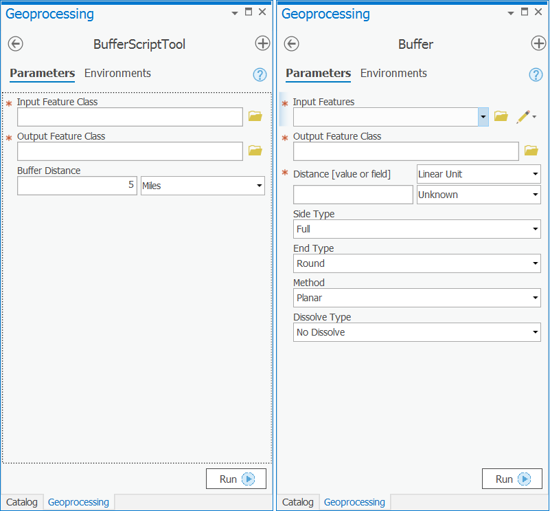
At some point, you may need to design a set of tools for beginning GIS users where only the most necessary parameters are exposed. You may also do this to enforce quality control if you know that some of the parameters must always be set to certain defaults, and you want to avoid the scenario where a beginning user (or a rogue user) might change the required values. A simple script tool is effective for simplifying the tool dialog in this way.
Readings
ArcGIS Pro edition:
Read Zandbergen 3.9- 3.10 to reinforce what you learned during this lesson about scripts and script tools.
Lesson 1 Practice Exercises
Each lesson in this course includes some simple practice exercises with Python. These are not submitted or graded, but they are highly recommended if you are new to programming or if the project initially looks challenging. Lessons 1 and 2 contain shorter exercises, while Lessons 3 and 4 contain longer, more holistic exercises. Each practice exercise has an accompanying solution that you should carefully study. If you want to use the USA.gdb referenced in some of the solutions you can find it here. [13]
Remember to choose File > New in PyScripter to create a new script (or click the empty page icon). You can name the scripts something like Practice1, Practice2, etc. To execute a script in PyScripter, click the "play" icon.
- Say hello
Create a string variable called x and assign it the value "Hello". Display the contents of the x variable in the Console.
Practice 1 Solution [17] - Concatenate two strings
Create a string variable called first and assign to it your first name. Likewise, create a string variable called last and assign to it your last name. Concatenate (merge) the two strings together, making sure to also include a space between them.
Practice 2 Solution [18] - Pass a value to a script as a parameter
Example 1.6.4 shows the use of the arcpy.GetParameterAsText() function. This function is typically used in conjunction with an ArcGIS script tool that has been designed to prompt the user to enter the required parameters. However, it is possible to supply arguments to the script from within PyScripter. To do so, you would select Run > Configuration per file, check the Command line options checkbox, then enter the arguments something like this:
C:\PSU\geog485\Lesson1\us_cities.shp C:\PSU\geog485\Lesson1\us_cities_buffered.shp "10 miles"
Note that the arguments to the two feature class parameters are unquoted, while the argument to the buffer distance string parameter is provided in double quotes.
For this exercise, write a script that accepts a single string value using the GetParameterAsText method. The value entered should be a name, and that name should be concatenated with the literal string "Hi, " and displayed in the console. Test the script from within PyScripter, entering a name (in double quotes) in the Command line options text box as outlined above prior to clicking the Run button.
Practice 3 Solution [19] - Report the geometry type of a feature class
Example 1.6.2 demonstrates the use of the Describe function to report the spatial reference of a feature class. The Describe function returns an object that has a number of properties that can vary depending on what type of object you Described. A feature class has a spatialReference property by virtue of the fact that it is a type of Dataset. (Rasters are another type of Dataset and also have a spatialReference property.)
The Describe function's page in the Help [20] lists the types of objects that the function can be used on. Clicking the Dataset properties link pulls up a list of the properties available when you Describe a dataset, spatialReference being just one of several.
For this exercise, use the Describe function again; this time, to determine the type of geometry (point, polyline or polygon) stored in a feature class. I won't tell you the name of the property that returns this information. But I will give you the hint that feature classes have this mystery property not because they're a type of Dataset as with the spatialReference property, but because they're objects of the type FeatureClass.
Practice 4 Solution [21] - Do some simple math and report your results
Create a variable score1 and assign it a value of 90. Then create a variable score2 and assign it a value of 80. Compute the sum and average of these values and output to the Console the following messages, filling in the blanks:
The sum of these scores is ______.
Their average is ______.
In constructing your messages, you're probably going to want concatenate text strings with numbers. We'll cover this more in Lesson 2, but this requires converting the numeric values into strings to avoid a syntax error. The str() function can be used to do this conversion. For example, I might output the score1 value like this:
print('Score 1 is ' + str(score1))
Practice 5 Solution [22]
Project 1, Part 1: Modeling precipitation zones in Nebraska
Suppose you're working on a project for the Nebraska Department of Agriculture and you are tasked with making some maps of precipitation in the state. Members of the department want to see which parts of the state were relatively dry and wet in the past year, classified in zones. All you have is a series of weather station readings of cumulative rainfall for 2008 that you've obtained from within Nebraska and surrounding areas. This is a shapefile of points called Precip2008Readings.shp. It is in your Lesson 1 data folder.
Precip2008Readings.shp is a fictional dataset created for this project. The locations do not correspond to actual weather stations. However, the measurements are derived from real 2008 precipitation data created by the PRISM Climate Group [23] at Oregon State University.
You need to do several tasks in order to get this data ready for mapping:
- Interpolate a precipitation surface from your points. This creates a raster dataset with estimated precipitation values for your entire area of interest. You've already planned for this, knowing that you are going to use inverse distance weighted (IDW) interpolation. Click the following link to learn how the IDW technique works. [24] You've also selected your points to include some areas around Nebraska to avoid edge effects in the interpolation.
- Reclassify the interpolated surface into an ordinal classification of precipitation "zones" that delineate relatively dry, medium, and wet regions.
- Create vector polygons from the zones.
- Clip the zone polygons to the boundary of Nebraska.
 Figure 1.15 Mapping the data.
It's very possible that you'll want to repeat the above process in order to test different IDW interpolation parameters or make similar maps with other datasets (such as next year's precipitation data). Therefore, the above series of tasks is well-suited to ModelBuilder. Your job is to create a model that can complete the above series of steps without you having to manually open four different tools.
Model parameters
Your model should have these (and only these) parameters:
- Input precipitation readings- This is the location of your precipitation readings point data. This is a model parameter so that the model can be easily re-run with other datasets.
- Power- An IDW setting specifying how quickly influence of surrounding points decreases as you move away from the point to be interpolated.
- Search radius- An IDW setting determining how many surrounding points are included in the interpolation of a point. The search radius can be fixed at a certain distance, including whatever number of points happen to fall within, or its distance can vary in order for it to always include a minimum number of points. When you use ModelBuilder, you don't have to set up any of these choices; ModelBuilder does it for you when you set the Search Radius as a model parameter.
- Zone boundaries- This is a table allowing the user of the model to specify the zone boundaries. By default, the table should be configured as shown in Figure 1.16 below: Precipitation values of 0 - 30000 will result in a reclassification of 1 (to correspond with Zone 1), 30000 - 60000 will result in a classification of 2 (to correspond with Zone 2), and so on. The way to get this table is to make a variable from the Reclassification parameter of the Reclassify tool and set it as a model parameter.
- Output precipitation zones- This is the location where you want the output dataset of clipped vector zones to be placed on disk.
As you build your model, you will need to configure some settings that will not be exposed as parameters. These include the clip feature, which is the state of Nebraska outline Nebraska.shp in your Lesson 1 data folder. There are many other settings such as "Z Value field" and "Input barrier polyline features" (for IDW) or "Reclass field" (for Reclassify) that should not be exposed as parameters. You should just set these values once when you build your model. If you ever ask someone else to run this model, you don't want them to be overwhelmed with choices stemming from every tool in the model; you should just expose the essential things they might want to change.
For this particular model, you should assume that any input dataset will conform to the same schema as your Precip2008Readings.shp feature class. For example, an analyst should be able to submit similar datasets Precip2009Readings, Precip2010Readings, etc. for more recent years with the same fields, field names, and data types. However, he or she should not expect to provide any feature class with a different set of fields and field names, etc. As you might discover, handling all types of feature class schemas would make your model more complex than we want for this assignment.
Important: Given the scenario of wishing to re-run the model for other years of data, it would be a good idea to set default values for the exposed model parameters. Therefore, we are asking you to set default values for all parameters that are exposed as model parameters including the Power value, Search radius value, and Zone boundaries classification table. When you double-click the model to run it, the interface should look like the following:

Running the model with the exact parameters listed above should result in the following (I have symbolized the zones in Pro with different colors to help distinguish them). This is one way you can check your work:

Once you are done, take a screenshot of the layout of your final model in ModelBuilder (similar to Figure 1.5 in Section 1.3.2) to include in your homework submission.
Tips
The following tips may help you as you build your model:
- Your model needs to include the following tools in this order: IDW (from the Spatial Analyst toolbox), Reclassify, Raster to Polygon, Clip (from the Analysis toolbox).
- An easy way to find the tools you need in Pro is to go to Analysis > Tools, then type the name of the tool you want in the search box. Be careful when multiple tools have the same name. You'll typically be using tools from the Spatial Analyst toolbox in this assignment.
- Once you drag and drop a tool onto the ModelBuilder canvas, double-click it and set all the parameters the way you want. These will be the default settings for your model.
- If there is a certain parameter for a tool that you want to expose as a model parameter, right-click the tool in the ModelBuilder canvas, then click Create Variable > From Parameter and choose the parameter. Once the oval appears for the variable, right-click it and click Parameter.
Project 1, Part II: Creating contours for the Fox Lake DEM
The second part of Project 1 will help you get some practice with Python. At the end of Lesson 1, you saw three simple scripting examples; now your task is to write your own script. This script will create vector contour lines from a raster elevation dataset. Don't forget that the ArcGIS Pro Help [25] can indeed be helpful if you need to figure out the syntax for a particular command.
Earlier in the lesson, you were introduced to the Fox Lake DEM in your Lesson 1 data folder. It represents elevation in the Fox Lake Quadrangle, Utah. Write a script that uses the Contour tool in the Spatial Analyst toolbox to create contour lines for the quadrangle. The contour interval should be 25 meters, and the base contour should be 0. Remember that the native units of the DEM are meters, so no unit conversions are required.
Running the script should immediately create a shapefile of contour lines on disk.
Follow these guidelines when writing the script:
- The purpose of this exercise is just to get you some practice writing Python code. Therefore, you are not required to use arcpy.GetParameterAsText() to get the input parameters. Go ahead and hard-code the values (such as the path name to the dataset).
- Consequently, you are not required to create a script tool for this exercise. This will be required in Project 2.
- Your code should run correctly from PyScripter. For full credit, it should also contain comments, attempt to handle errors, and use legal and intuitive variable names.
- You should assume that you're writing your script for an organization that has a limited number of concurrent Spatial Analyst licenses available.
Deliverables
The deliverables for Project 1 are:
- The .atbx file of the toolbox containing your Part I model. The easiest way to find it is to hover your mouse over the toolbox in the Catalog window and note its location in the box that appears.
- A screenshot showing the layout of your final model for Part 1 (the model in the ModelBuilder editor, not the tool interface and not the produced output of your model).
- The .py file containing your Part II script.
- A short writeup (about 400 words) describing how you approached the two problems, any setbacks you faced, and how you dealt with those. These writeups will be required on all projects.
Important: Successful delivery of the above requirements is sufficient to earn 90% on the project. The remaining 10% is reserved for efforts that go "over and above" the minimum requirements. For Part I, this could include (but is not limited to) analysis of how different input values affect the output, substitution of some other interpolation method instead of IDW (for example Kriging), documentation for your model parameters that guides the end user in what to input, or demonstration of how your model was successfully run on a different input dataset. For Part II, in addition to the Contour tool, you could run some other tool that also takes a DEM as an input.
As a general rule throughout the course, full credit in the "over and above" category requires the implementation of 2-4 different ideas, with more complex ideas earning more credit. Note that for future projects, we won't be listing off ideas as we've done here. Otherwise, it wouldn't really be an over and above requirement. ![]()
Finishing Lesson 1
To complete Lesson 1, please zip all your Project 1 deliverables (for parts I and II) into one file and submit them to the Project 1 Drop Box in Canvas. Then take the Lesson 1 Quiz if you haven't taken it already.
Lesson 2: Python and programming basics
The links below provide an outline of the material for this lesson. Be sure to carefully read through the entire lesson before returning to Canvas to submit your assignments.
Lesson 2 Overview
In Lesson 1, you received an introduction to Python. Lesson 2 builds on that experience, diving into Python fundamentals. Many of the things you'll learn are common to programming in other languages. If you already have coding experience, this lesson may contain some review.
This lesson has a relatively large amount of reading from the course materials, the Zandbergen text, and the ArcGIS help. I believe you will get a better understanding of the Python concepts as they are explained and demonstrated from several different perspectives. Whenever the examples use the IPython console, I strongly suggest that you type in the code yourself as you follow the examples. This can take some time, but you'll be amazed at how much more information you retain if you try the examples yourself instead of just reading them.
At the end of the lesson, you'll be required to write a Python script that puts together many of the things you've learned. This will go much faster if you've taken the time to read all the required text and work through the examples.
Lesson 2 Checklist
Lesson 2 covers Python fundamentals (many of which are common to other programming languages) and gives you a chance to practice these in a project. To complete this lesson, you are required to do the following:
- Download the Lesson 2 data [26] and extract it to C:\PSU\Geog485\Lesson2.
- Work through the online sections of the lesson.
- Read the remainder of Zandbergen chapters 4-6 that we didn't cover in Lesson 1 and sections 7.1 - 7.5. In the online lesson pages, I have inserted instructions about when it is most appropriate to read each of these chapters. There is more reading in this lesson than in a typical week. If you are new to Python, please plan some extra time to read these chapters. There are also some readings this week from the ArcGIS Help.
- Complete Project 2 and upload its deliverables to the Lesson 2 drop box in Canvas. The deliverables are listed in the Project 2 description page.
- Complete the Lesson 2 Quiz in Canvas.
Do items 1 - 3 (including any of the practice exercises you want to attempt) during the first week of the lesson. You will need the second week to concentrate on the project and quiz.
Lesson objectives
By the end of this lesson, you should:
- understand basic Python syntax for conditional statements and program flow control (if-else, comparison operators, for loop, while loop);
- be familiar with more advanced data types (strings, lists), string manipulation, and casting between different types;
- know how to debug code and how to use the debugger;
- be able to program basic scripts that use conditional statements and loops to automate tasks.
2.1 More Python fundamentals
At this point, you've learned most of what you need to know about ModelBuilder, and this may be enough to address many of the GIS tasks that you face in your work. However, as useful as ModelBuilder is, you'll find that sometimes you need Python to build extra intelligence into your geoprocessing. For example, you may need to construct complex query strings, or employ conditional logic. You may need to read, or parse, varying types of user input before you can send it to a tool as a parameter. Or you might need to do complex looping that, at some threshold, probably becomes easier to write in Python than to figure out with ModelBuilder.
In Lesson 1, you saw your first Python scripts and were introduced to the basics, such as importing modules, using arcpy, working with properties and methods, and indenting your code in try/catch blocks. In the following sections, you'll learn about more Python programming fundamentals such as working with lists, looping, if/then decision structures, manipulating strings, and casting variables.
Although this might not be the most thrilling section of the course, it's probably the most important section for you to spend time understanding and experimenting with on your own, especially if you are new to programming.
Programming is similar to playing sports: if you take time to practice the fundamentals, you'll have an easier time when you need to put all your skills together. For example, think about the things you need to learn in order to play basketball. A disciplined basketball player practices dribbling, passing, long-range shooting, layup shots, free throws, defense, and other skills. If you practice each of these fundamentals well individually, you'll be able to put them together when it's time to play a full game.
Learning a programming language is the same way. When faced with a problem, you'll be forced to draw on your fundamental skills to come up with a workable plan. You may need to include a loop in your program, store items in a list, or make the program do one of four different things based on certain user input. If you know how to do each of these things individually, you'll be able to fit the pieces together, even if the required task seems daunting.
Take time to make sure you understand what's happening in each line of the code examples, and if you run into a question, please jot it down and post to the forums.
2.1.1 Lists
In Lesson 1, you learned about some common data types in Python, such as strings and integers. Sometimes you need a type that can store multiple related values together. Python offers several ways of doing this, and the first one we'll learn about is the list.
Here's a simple example of a list. You can type this in the PyScripter Python Interpreter to follow along:
>>> suits = ['Spades', 'Clubs', 'Diamonds', 'Hearts']
This list named 'suits' stores four related string values representing the suits in a deck of cards. In many programming languages, storing a group of objects in sequence like this is done with arrays. While the Python list could be thought of as an array, it's a little more flexible than the typical array in other programming languages. This is because you're allowed to put multiple data types into one list.
For example, suppose we wanted to make a list for the card values you could draw. The list might look like this:
>>> values = ['Ace', 2, 3, 4, 5, 6, 7, 8, 9, 10, 'Jack', 'Queen', 'King']
Notice that you just mixed string and integer values in the list. Python doesn't care. However, each item in the list still has an index, meaning an integer that denotes each item's place in the list. The list starts with index 0 and for each item in the list, the index increments by one. Try this:
>>> print (suits[0])
Spades
>>> print (values[12])
King
In the above lines, you just requested the item with index 0 in the suits list and got 'Spades'. Similarly, you requested the item with index 12 in the values list and got 'King'.
It may take some practice initially to remember that your lists start with a 0 index. Testing your scripts can help you avoid off-by-one errors that might result from forgetting that lists are zero-indexed. For example, you might set up a script to draw 100 random cards and print the values. If none of them is an Ace, you've probably stacked the deck against yourself by making the indices begin at 1.
Remember you learned that everything is an object in Python? That applies to lists too. In fact, lists have a lot of useful methods that you can use to change the order of the items, insert items, sort the list, and so on. Try this:
>>> suits = ['Spades', 'Clubs', 'Diamonds', 'Hearts']
>>> suits.sort()
>>> print (suits)
['Clubs', 'Diamonds', 'Hearts', 'Spades']
Notice that the items in the list are now in alphabetical order. The sort() method allowed you to do something in one line of code that would have otherwise taken many lines. Another helpful method like this is reverse(), which allows you to sort a list in reverse alphabetical order:
>>> suits.reverse()
>>> print (suits)
['Spades', 'Hearts', 'Diamonds', 'Clubs']
Before you attempt to write list-manipulation code, check your textbook or the Python list reference documentation [27] to see if there's an existing method that might simplify your work.
Inserting items and combining lists
What happens when you want to combine two lists? Type this in the PyScripter Interpreter:
>>> listOne = [101,102,103]
>>> listTwo = [104,105,106]
>>> listThree = listOne + listTwo
>>> print (listThree)
[101, 102, 103, 104, 105, 106]
Notice that you did not get [205,207,209]; rather, Python treats the addition as appending listTwo to listOne. Next, try these other ways of adding items to the list:
>>> listThree += [107]
>>> print (listThree)
[101, 102, 103, 104, 105, 106, 107]
>>> listThree.append(108)
>>> print (listThree)
[101, 102, 103, 104, 105, 106, 107, 108]
To put an item at the end of the list, you can either add a one-item list (how we added 107 to the list) or use the append() method on the list (how we added 108 to the list). Notice that listThree += [107] is a shortened form of saying listThree = listThree + [107].
If you need to insert some items in the middle of the list, you can use the insert() method:
>>> listThree.insert(4, 999)
>>> print (listThree)
[101, 102, 103, 104, 999, 105, 106, 107, 108]
Notice that the insert() method above took two parameters. You might have even noticed a tooltip that shows you what the parameters mean.
The first parameter is the index position that the new item will take. This method call inserts 999 between 104 and 105. Now 999 is at index 4.
Getting the length of a list
Sometimes you'll need to find out how many items are in a list, particularly when looping. Here's how you can get the length of a list:
>>> myList = [4,9,12,3,56,133,27,3]
>>> print (len(myList))
8
Notice that len() gives you the exact number of items in the list. To get the index of the final item, you would need to use len(myList) - 1. Again, this distinction can lead to off-by-one errors if you're not careful.
Other ways to store collections of data
Lists are not the only way to store ordered collections of items in Python; you can also use tuples and dictionaries. Tuples are like lists, but you can't change the objects inside a tuple over time. In some cases, a tuple might actually be a better structure for storing values like the suits in a deck of cards because this is a fixed list that you wouldn't want your program to change by accident.
Dictionaries differ from lists in that items are not indexed; instead, each item is stored with a key value which can be used to retrieve the item. We'll use dictionaries later in the course, and your reading assignment for this lesson covers dictionary basics. The best way to understand how dictionaries work is to play with some of the textbook examples in the PyScripter Python Interpreter (see Zandbergen 4.17).
2.1.2 Loops
A loop is a section of code that repeats an action. Remember, the power of scripting (and computing in general) is the ability to quickly repeat a task that might be time-consuming or error-prone for a human. Looping is how you repeat tasks with code; whether its reading a file, searching for a value, or performing the same action on each item in a list.
for Loop
A for loop does something with each item in a list. Type this in the PyScripter Python Interpreter to see how a simple for loop works:
>>> for name in ["Carter", "Reagan", "Bush"]:
 	print (name + " was a U.S. president.")
After typing this, you'll have to hit Enter twice in a row to tell PyScripter that you are done working on the loop and that the loop should be executed. You should see:
Carter was a U.S. president
Reagan was a U.S. president
Bush was a U.S. president
Notice a couple of important things about the loop above. First, you declared a new variable, "name," to represent each item in the list as you iterated through. This is okay to do; in fact, it's expected that you'll do this at the beginning of the for loop.
The second thing to notice is that after the condition, or the first line of the loop, you typed a colon (:), then started indenting subsequent lines. Some programming languages require you to type some kind of special line or character at the end of the loop (for example, "Next" in Visual Basic, or "}" in JavaScript), but Python just looks for the place where you stop indenting. By pressing Enter twice, you told Python to stop indenting and that you were ready to run the loop.
for loops can also work with lists of numbers. Try this one in the PyScripter Python Interpreter:
>>> x = 2
>>> multipliers = [1,2,3,4]
>>> for num in multipliers:
 	print (x * num)

2
4
6
8
In the loop above, you multiplied each item in the list by 2. Notice that you can set up your list before you start coding the loop.
You could have also done the following with the same result:
>>> multipliers = [1,2,3,4]
>>> for num in multipliers:
 	x = 2
 	print (x * num)
The above code, however, is less efficient than what we did initially. Can you see why? This time, you are declaring and setting the variable x=2 inside the loop. The Python interpreter will now have to read and execute that line of code four times instead of one. You might think this is a trivial amount of work, but if your list contained thousands or millions of items, the difference in execution time would become noticeable. Declaring and setting variables outside a loop, whenever possible, is a best practice in programming.
While we're on the subject, what would you do if you wanted to multiply 2 by every number from 1 to 1000? It would definitely be too much typing to manually set up a multipliers list, as in the previous example. In this case, you can use Python's built-in range function. Try this:
>>> x = 2
>>> for num in range(1,1001):
 	print (x * num)
The range function is your way of telling Python, "Start here and stop there." We used 1001 because the loop stops one item before the function's second argument (the arguments are the values you put in parentheses to tell the function how to run). If you need the function to multiply by 0 at the beginning as well, you could even get away with using one argument:
>>> x = 2
>>> for num in range(1001):
 	 print (x * num)
The range function has many interesting uses, which are detailed in this section's reading assignment in Zandbergen.
while Loops
A while loop executes until some condition is met. Here's how to code our example above using a while loop:
>>> x = 0
>>> while x < 1001:
 	 print (x * 2)
         x += 1
while loops often involve the use of some counter that keeps track of how many times the loop has run. Sometimes you'll perform operations with the counter. For example, in the above loop, x was the counter, and we also multiplied the counter by 2 each time during the loop. To increment the counter, we used x += 1 which is shorthand for x = x + 1, or "add one to x".
Nesting loops
Some situations call for putting one loop inside another, a practice called nesting. Nested loops could help you print every card in a deck (minus the Jokers):
>>> suits = ['Spades', 'Clubs', 'Diamonds', 'Hearts']
>>> values = ['Ace', 2, 3, 4, 5, 6, 7, 8, 9, 10, 'Jack', 'Queen', 'King']
>>> for suit in suits:
 	 for value in values:
 	     print (str(value) + " of " + str(suit))
In the above example, you start with a suit, then loop through each value in the suit, printing out the card name. When you've reached the end of the list of values, you jump out of the nested loop and go back to the first loop to get the next suit. Then you loop through all values in the second suit and print the card names. This process continues until all the suits and values have been looped through.
Looping in GIS models
You will use looping repeatedly (makes sense!) as you write GIS scripts in Python. Often, you'll need to iterate through every row in a table, every field in a table, or every feature class in a folder or a geodatabase. You might even need to loop through the vertices of a geographic feature.
You saw above that loops work particularly well with lists. arcpy has some methods that can help you create lists. Here's an example you can try that uses arcpy.ListFeatureClasses(). First, manually create a new folder C:\PSU\Geog485\Lesson2\PracticeData. Then copy the code below into a new script in PyScripter and run the script. The script copies all the data in your Lesson2 folder into the new Lesson2\PracticeData folder you just created.
1 2 3 4 5 6 7 8 9 10 11 12 13 14 15 16 | # Copies all feature classes from one folder to anotherimport arcpytry: arcpy.env.workspace = "C:/PSU/Geog485/Lesson2" # List the feature classes in the Lesson 2 folder fcList = arcpy.ListFeatureClasses() # Loop through the list and copy the feature classes to the Lesson 2 PracticeData folder for featureClass in fcList: arcpy.CopyFeatures_management(featureClass, "C:/PSU/Geog485/Lesson2/PracticeData/" + featureClass)except: print ("Script failed to complete") print (arcpy.GetMessages(2)) |
Notice above that once you have a Python list of feature classes (fcList), it's very easy to set up the loop condition (for featureClass in fcList:).
Another common operation in GIS scripts is looping through tables. In fact, the arcpy module contains some special objects called cursors that help you do this. Here's a short script showing how a cursor can loop through each row in a feature class and print the name. We'll cover cursors in detail in the next lesson, so don't worry if some of this code looks confusing right now. The important thing is to notice how a loop is used to iterate through each record:
1 2 3 4 5 6 7 8 9 10 11 12 | import arcpyinTable = "C:/PSU/Geog485/Lesson2/CityBoundaries.shp"inField = "NAME"rows = arcpy.SearchCursor(inTable)#This loop goes through each row in the table# and gets a requested field valuefor row in rows: currentCity = row.getValue(inField) print (currentCity) |
In the above example, a search cursor named rows retrieves records from the table. The for loop makes it possible to perform an action on each individual record.
ArcGIS Help reading
Read the following in the ArcGIS Pro Help:
- Create lists of data [28]
2.1.3 Decision structures
Many scripts that you write will need to have conditional logic that executes a block of code given a condition and perhaps executes a different block of code given a different condition. The "if," "elif," and "else" statements in Python provide this conditional logic. Try typing this example in the Python Interpreter:
>>> x = 3
>>> if x > 2:
 	    print ("Greater than two")

Greater than two
In the above example, the keyword "if" denotes that some conditional test is about to follow. In this case, the condition of x being greater than two was met, so the script printed "Greater than two." Notice that you are required to put a colon (:) after the condition and indent any code executing because of the condition. For consistency in this class, all indentation is done using four spaces.
Using "else" is a way to run code if the condition isn't met. Try this:
>>> x = 1
>>> if x > 2:
            print ("Greater than two")
        else:
            print ("Less than or equal to two")

Less than or equal to two
Notice that you don't have to put any condition after "else." It's a way of catching all other cases. Again, the conditional code is indented four spaces, which makes the code very easy for a human to scan. The indentation is required because Python doesn't require any type of "end if" statement (like many other languages) to denote the end of the code you want to execute.
If you want to run through multiple conditions, you can use "elif", which is Python's abbreviation for "else if":
>>> x = 2
>>> if x > 2:
            print ("Greater than two")
        elif x == 2:
            print ("Equal to two")
        else:
            print ("Less than two")

Equal to two
In the code above, elif x == 2: tests whether x is equal to two. The == is a way to test whether two values are equal. Using a single = in this case would result in an error because = is used to assign values to variables. In the code above, you're not trying to assign x the value of 2, you want to check if x is already equal to 2, hence you use ==.
Caution: Using = instead of == to check for equivalency is a very common Python mistake, especially if you've used other languages where = is allowed for equivalency checks.
You can also use if, elif, and else to handle multiple possibilities in a set. The code below picks a random school from a list (notice we had to import the random module to do this and call a special method random.randrange()). After the school is selected and its name is printed, a series of if/elif/else statements appears that handles each possibility. Notice that the else statement is left in as an error handler; you should not run into that line if your code works properly, but you can leave the line in there to fail gracefully if something goes wrong.
1 2 3 4 5 6 7 8 9 10 11 12 13 14 15 16 17 18 19 | import random# Choose a random school from a list and print itschools = ["Penn State", "Michigan", "Ohio State", "Indiana"]randomSchoolIndex = random.randrange(0,4)chosenSchool = schools[randomSchoolIndex]print (chosenSchool)# Depending on the school, print the mascotif chosenSchool == "Penn State": print ("You're a Nittany Lion")elif chosenSchool == "Michigan": print ("You're a Wolverine")elif chosenSchool == "Ohio State": print ("You're a Buckeye")elif chosenSchool == "Indiana": print ("You're a Hoosier")else: print ("This program has an error") |
Another way to handle the conditional logic above is to employ Python's match/case approach. To try this approach, replace the if block in the bottom half of the script with the snippet below:
1 2 3 4 5 6 7 8 9 10 11 12 | # Depending on the school, print the mascotmatch chosenSchool: case "Penn State": print ("You're a Nittany Lion") case "Michigan": print ("You're a Wolverine") case "Ohio State": print ("You're a Buckeye") case "Indiana": print ("You're a Hoosier") case _: print ("This program has an error") |
2.1.4 String manipulation
You've previously learned how the string variable can contain numbers and letters and represent almost anything. When using Python with ArcGIS, strings can be useful for storing paths to data and printing messages to the user. There are also some geoprocessing tool parameters that you'll need to supply with strings.
Python has some very useful string manipulation abilities. We won't get into all of them in this course, but the following are a few techniques that you need to know.
Concatenating strings
To concatenate two strings means to append or add one string on to the end of another. For example, you could concatenate the strings "Python is " and "a scripting language" to make the complete sentence "Python is a scripting language." Since you are adding one string to another, it's intuitive that in Python you can use the + sign to concatenate strings.
You may need to concatenate strings when working with path names. Sometimes it's helpful or required to store one string representing the folder or geodatabase from which you're pulling datasets and a second string representing the dataset itself. You put both together to make a full path.
The following example, modified from one in the ArcGIS Help, demonstrates this concept. Suppose you already have a list of strings representing feature classes that you want to clip. The list is represented by "featureClassList" in this script:
1 2 3 4 5 6 7 8 9 10 11 12 13 14 15 16 17 18 | # This script clips all datasets in a folderimport arcpyinFolder = "c:\\data\\inputShapefiles\\"resultsFolder = "c:\\data\\results\\"clipFeature = "c:\\data\\states\\Nebraska.shp"# List feature classesarcpy.env.workspace = inFolderfeatureClassList = arcpy.ListFeatureClasses()# Loop through each feature class and clipfor featureClass in featureClassList: # Make the output path by concatenating strings outputPath = resultsFolder + featureClass # Clip the feature class arcpy.Clip_analysis(featureClass, clipFeature, outputPath) |
String concatenation is occurring in this line: outputPath = resultsFolder + featureClass. In longhand, the output folder "c:\\data\\results\\" is getting the feature class name added on the end. If the feature class name were "Roads.shp" the resulting output string would be "c:\\data\\results\\Roads.shp".
The above example shows that string concatenation can be useful in looping. Constructing the output path by using a set workspace or folder name followed by a feature class name from a list gives much more flexibility than trying to create output path strings for each dataset individually. You may not know how many feature classes are in the list or what their names are. You can get around that if you construct the output paths on the fly through string concatenation.
Casting to a string
Sometimes in programming, you have a variable of one type that needs to be treated as another type. For example, 5 can be represented as a number or as a string. Python can only perform math on 5 if it is treated as a number, and it can only concatenate 5 onto an existing string if it is treated as a string.
Casting is a way of forcing your program to think of a variable as a different type. Create a new script in PyScripter, and type or paste the following code:
1 2 3 4 5 6 | x = 0while x < 10: print (x) x += 1print ("You ran the loop " + x + " times.") |
Now, try to run it. The script attempts to concatenate strings with the variable x to print how many times you ran a loop, but it results in an error: "TypeError: must be str not int." Python doesn't have a problem when you want to print the variable x on its own, but Python cannot mix strings and integer variables in a printed statement. To get the code to work, you have to cast the variable x to a string when you try to print it.
1 2 3 4 5 6 | x = 0while x < 10: print (x) x += 1print ("You ran the loop " + str(x) + " times.") |
You can force Python to think of x as a string by using str(x). Python has other casting functions such as int() and float() that you can use if you need to go from a string to a number. Use int() for integers and float() for decimals.
Readings
It's time to take a break and do some readings from another source. If you are new to Python scripting, this will help you see the concepts from a second angle.
Finish reading Zandbergen chapters 4 - 6 as detailed below. This can take a few hours, but it will save you hours of time if you make sure you understand this material now.
ArcGIS Pro edition:
- Chapter 4 covers the basics of Python syntax, loops, strings, and other things we just learned. Please read Chapter 4, noting the following:
- You were already assigned 4.1-4.7 in Lesson 1, so you may skip those sections if you have a good handle on those topics.
- You may also skip 4.17-4.18, and 4.26.
- Section 4.25 demonstrates use of the input() function, using the IDLE and PyCharm IDEs. IDEs vary in their implementation of the type() function. In PyScripter, the user is expected to enter a value in the PyScripter Python Interpreter.
- Another way of providing input to a script in PyScripter is by going to Run > Command Line Parameters, checking the Use Command line Parameters box, entering the arguments in the box that appears, then clicking Run. - You've already read most of Chapter 5 on geoprocessing with arcpy. Now please read 5.10 & 5.14.
- Chapter 6 gives some specific instructions about working with ArcGIS datasets, which will be valuable during this week's assigned project. Please read all sections, 6.1-6.7.
If you still don't feel like you understand the material after reading the above chapters, don't re-read it just yet. Try some coding from the Lesson 2 practice exercises and assignments, then come back and re-read if necessary. If you are really struggling with a particular concept, type the examples in the console. Programming is like a sport in the sense that you cannot learn all about it by reading; at some point, you have to get up and do it.
2.1.5 Putting it all together
In this section of the lesson, you've learned the basic programming concepts of lists, loops, decision structures, and string manipulation. You might be surprised at what you can do with just these skills. In this section, we'll practice putting them all together to address a scenario. This will give us an opportunity to talk about strategies for approaching programming problems in general.
The scenario we'll tackle is to simulate a one-player game of Hasbro's children's game "Hi Ho! Cherry-O." In this simple game of chance, you begin with 10 cherries on a tree. You take a turn by spinning a random spinner, which tells you whether you get to add or remove cherries on the turn. The possible spinner results are:
- Remove 1 cherry.
- Remove 2 cherries.
- Remove 3 cherries.
- Remove 4 cherries.
- Bird visits your cherry bucket (Add 2 cherries).
- Dog visits your cherry bucket (Add 2 cherries).
- Spilled bucket (Place all 10 cherries back on your tree).
You continue taking turns until you have 0 cherries left on your tree, at which point you have won the game. Your objective here is to write a script that simulates the game, printing the following:
- The result of each spin.
- The number of cherries on your tree after each turn. This must always be between 0 and 10;
- The final number of turns needed to win the game.
Approaching a programming problem
Although this example may seem juvenile, it's an excellent way to practice everything you just learned. As a beginner, you may seem overwhelmed by the above problem. A common question is, "Where do I start?" The best approach is to break down the problem into smaller chunks of things you know how to do.
One of the most important programming skills you can acquire is the ability to verbalize a problem and translate it into a series of small programming steps. Here's a list of things you would need to do in this script. Programmers call this pseudocode because it's not written in code, but it follows the sequence their code will need to take.
- Spin the spinner.
- Print the spin result.
- Add or remove cherries based on the result.
- Make sure the number of cherries is between 0 and 10.
- Print the number of cherries on the tree.
- Take another turn, or print the number of turns it took to win the game.
It also helps to list the variables you'll need to keep track of:
- Number of cherries currently on the tree (Starts at 10).
- Number of turns taken (Starts at 0).
- Value of the spinner (Random).
Let's try to address each of the pseudocode steps. Don't worry about the full flow of the script yet. Rather, try to understand how each step of the problem should be solved with code. Assembling the blocks of code at the end is relatively trivial.
Spin the spinner
How do you simulate a random spin? In one of our previous examples, we used the random module to generate a random number within a range of integers; however, the choices on this spinner are not linear. A good approach here is to store all spin possibilities in a list and use the random number generator to pick the index for one of the possibilities. On its own, the code would look like this:
1 2 3 4 | import randomspinnerChoices = [-1, -2, -3, -4, 2, 2, 10]spinIndex = random.randrange(0, 7)spinResult = spinnerChoices[spinIndex] |
The list spinnerChoices holds all possible mathematical results of a spin (remove 1 cherry, remove 2 cherries, etc.). The final value 10 represents the spilled bucket (putting all cherries back on the tree).
You need to pick one random value out of this list to simulate a spin. The variable spinIndex represents a random integer from 0 to 6 that is the index of the item you'll pull out of the list. For example, if spinIndex turns out to be 2, your spin is -3 (remove 3 cherries from the tree). The spin is held in the variable spinResult.
The random.randrange() method is used to pick the random numbers. At the beginning of your script, you have to import the random module in order to use this method.
Print the spin result
Once you have a spin result, it only takes one line of code to print it. You'll have to use the str() method to cast it to a string, though.
print ("You spun " + str(spinResult) + ".")
Add or remove cherries based on the result
As mentioned above, you need to have some variable to keep track of the number of cherries on your tree. This is one of those variables that it helps to name intuitively:
cherriesOnTree = 10
After you complete a spin, you need to modify this variable based on the result. Remember that the result is held in the variable spinResult, and that a negative spinResult removes cherries from your tree. So your code to modify the number of cherries on the tree would look like:
cherriesOnTree += spinResult
Remember, the above is shorthand for saying cherriesOnTree = cherriesOnTree + spinResult.
Make sure the number of cherries is between 0 and 10
If you win the game, you have 0 cherries. You don't have to reach 0 exactly, but it doesn't make sense to say that you have negative cherries. Similarly, you might spin the spilled bucket, which for simplicity we represented with positive 10 in the spinnerChoices. You are not allowed to have more than 10 cherries on the tree.
A simple if/elif decision structure can help you keep the cherriesOnTree within 0 and 10:
if cherriesOnTree > 10:
    cherriesOnTree = 10
elif cherriesOnTree < 0:
    cherriesOnTree = 0
This means, if you wound up with more than 10 cherries on the tree, set cherriesOnTree back to 10. If you wound up with fewer than 0 cherries, set cherriesOnTree to 0.
Print the number of cherries on the tree
All you have to do for this step is to print your cherriesOnTree variable, casting it to a string, so it can legally be inserted into a sentence.
print ("You have " + str(cherriesOnTree) + "cherries on your tree.")
Take another turn or print the number of turns it took to win the game
You probably anticipated that you would have to figure out a way to take multiple turns. This is the perfect scenario for a loop.
What is the loop condition? There have to be some cherries left on the tree in order to start another turn, so you could begin the loop this way:
while cherriesOnTree > 0:
Much of the code we wrote above would go inside the loop to simulate a turn. Since we need to keep track of the number of turns taken, at the end of the loop we need to increment a counter:
turns += 1
This turns variable would have to be initialized at the beginning of the script, before the loop.
This code could print the number of turns at the end of the game:
print ("It took you " + str(turns) + "turns to win the game.")
Final code
Your only remaining task is to assemble the above pieces of code into a script. Below is an example of how the final script would look. Copy this into a new PyScripter script and try to run it:
1 2 3 4 5 6 7 8 9 10 11 12 13 14 15 16 17 18 19 20 21 22 23 24 25 26 27 28 29 30 31 32 33 34 35 | # Simulates one game of Hi Ho! Cherry-Oimport randomspinnerChoices = [-1, -2, -3, -4, 2, 2, 10]turns = 0cherriesOnTree = 10# Take a turn as long as you have more than 0 cherrieswhile cherriesOnTree > 0: # Spin the spinner spinIndex = random.randrange(0, 7) spinResult = spinnerChoices[spinIndex] # Print the spin result print ("You spun " + str(spinResult) + ".") # Add or remove cherries based on the result cherriesOnTree += spinResult # Make sure the number of cherries is between 0 and 10 if cherriesOnTree > 10: cherriesOnTree = 10 elif cherriesOnTree < 0: cherriesOnTree = 0 # Print the number of cherries on the tree print ("You have " + str(cherriesOnTree) + " cherries on your tree.") turns += 1# Print the number of turns it took to win the gameprint ("It took you " + str(turns) + " turns to win the game.")lastline = input(">") |
Analysis of the final code
Review the final code closely and consider the following things.
The first thing you do is import whatever supporting modules you need; in this case, it's the random module.
Next, you declare the variables that you'll use throughout the script. Each variable has a scope, which determines how broadly it is used throughout the script. The variables spinnerChoices, turns, and cherriesOnTree are needed through the entire script, so they are declared at the beginning, outside the loop. Variables used throughout your entire program like this have global scope. On the other hand, the variables spinIndex and spinResult have local scope because they are used only inside the loop. Each time the loop runs, these variables are re-initialized and their values change.
You could potentially declare the variable spinnerChoices inside the loop and get the same end result, but performance would be slower because the variable would have to be re-initialized every time you ran the loop. When possible, you should declare variables outside loops for this reason.
If you had declared the variables turns or cherriesOnTree inside the loop, your code would have logical errors. You would essentially be starting the game anew on every turn with 10 cherries on your tree, having taken 0 turns. In fact, you would create an infinite loop because there is no way to remove 10 cherries during one turn, and the loop condition would always evaluate to true. Again, be very careful about where you declare your variables when the script contains loops.
Notice that the total number of turns is printed outside the loop once the game has ended. The final line lastline = input(">") gives you an empty cursor prompting for input and is just a trick to make sure the application doesn't disappear when it's finished (if you run the script from a command console).
Summary
In the above example, you saw how lists, loops, decision structures, and variable casting can work together to help you solve a programming challenge. You also learned how to approach a problem one piece at a time and assemble those pieces into a working script. You'll have a chance to practice these concepts on your own during this week's assignment. The next and final section of this lesson will provide you with some sources of help if you get stuck.
Challenge activity
If the above activity made you enthusiastic about writing some code yourself, take the above script and try to find the average number of turns it takes to win a game of Hi-Ho! Cherry-O. To do this, add another loop that runs the game a large number of times, say 10000. You'll need to record the total number of turns required to win all the games, then divide by the number of games (use "/" for the division). Send me your final result, and I'll let you know if you've found the correct average.
2.2 Troubleshooting and getting help
If you find writing code to be a slow, mystifying, and painstaking process, fraught with all kinds of opportunities to make mistakes, welcome to the world of a programmer! Perhaps to their chagrin, programmers spend the majority of their time hunting down and fixing bugs. Programmers also have to continually expand and adapt their skills to work with new languages and technologies, which requires research, practice, and lots of trial and error.
The best candidates for software engineering jobs are not the ones who list the most languages or acronyms on their resumes. Instead, the most desirable candidates are self-sufficient, meaning they know how to learn new things and find answers to problems on their own. This doesn't mean that they never ask for help; on the contrary, a good programmer knows when to stop banging his or her head against the wall and consult peers or a supervisor for advice. However, most everyday problems can be solved using the help documentation, online code examples, online forums, existing code that works, programming books, and debugging tools in the software.
Suppose you're in a job interview and your prospective employer asks, "What do you do when you run into a 'brick wall' when programming? What sources do you first go to for help?" If you answer, "My supervisor" or "My co-workers," this is a red flag, signifying that you could be a potential time sink to the development team. Although the more difficult problems require group collaboration, a competitive software development team cannot afford to hold an employee's hand through every issue that he or she encounters. From the author's experience, many of the most compelling candidates answer this question, "Google." They know that most programming problems, although vexing, are common and the answer may be at their fingertips in less than 30 seconds through a well-phrased Internet search. With popular online forums such as Stack Exchange providing answers to many common syntax and structuring questions, searching for information online can actually be faster than walking down the hall and asking a co-worker, and it saves everybody time.
In this section of the lesson, you'll learn about places where you can go for help when working with Python and when programming in general. You will have a much easier experience in this course if you remember these resources and use them as you complete your assignments.
2.2.1 Potential problems and quick diagnosis
The secret to successful programming is to run early, run often, and don't be afraid of things going wrong when you run your code the first time. Debugging, or finding mistakes in code, is a part of life for programmers. Here are some things that can happen:
- Your code doesn't run at all, usually because of a syntax error (you typed some illegal Python code).
- Your code runs, but the script doesn't complete and reports an error.
- Your code runs, but the script never completes. Often this occurs when you've created an infinite loop.
- Your code runs and the script completes, but it doesn't give you the expected result. This is called a logical error, and it is often the type of error that takes the most effort to debug.
Don't be afraid of errors
Errors happen. There are very few programmers who can sit down and, off the top of their heads, write dozens of lines of bug free code. This means a couple of things for you:
- Expect to spend some time dealing with errors during the script-writing process. Beginning programmers sometimes underestimate how much time this takes. To get an initial estimate, you can take the amount of time it takes to draft your lines of code, then double it or triple it to accommodate for error handling and final polishing of your script and tool.
- Don't be afraid to run your script and hit the errors. A good strategy is to write a small piece of functionality, run it to make sure it's working, then add on the next piece. For the sake of discussion, let's suppose that as a new programmer, you introduce a new bug once every 10 lines of code. It's much easier to find a single bug in 10 new lines of code than it is to find 5 bugs in 50 new lines of code. If you're building your script piece by piece and debugging often, you'll be able to make a quicker and more accurate assessment of where you introduced new errors.
Catching syntax errors
Syntax errors occur when you typed something incorrectly and your code refuses to run. Common syntax errors include forgetting a colon when setting a loop or an if condition, using single backslashes in a file name, providing the wrong number of arguments to a function, or trying to mix variable types incorrectly, such as dividing a number by a string.
When you try to run code with a syntax error in PyScripter, an error message will appear in the Python Interpreter, referring to the script file that was run, along with the line number that contained the error. For example, a developer transitioning from ArcMap to ArcGIS Pro might forget that the syntax of the print function is different, resulting in the error message, "SyntaxError: Missing parentheses in call to 'print'. Did you mean print(x)?"
Dealing with crashes
If your code crashes, you may see an error message in the Python Interpreter. Instead of allowing your eyes to glaze over or banging your head against the desk, you should rejoice at the fact that the software possibly reported to you exactly what went wrong! Scour the message for clues as to what line of code caused the error and what the problem was. Do this even if the message looks intimidating. For example, see if you can understand what caused this error message (as reported by the Spyder IDE):
  runfile('C:/Users/detwiler/Documents/geog485/Lesson2/syntax_error_practice.py', wdir='C:/Users/detwiler/Documents/geog485/Lesson2')
Traceback (most recent call last):

  File ~\AppData\Local\ESRI\conda\envs\arcgispro-py3-spyd\lib\site-packages\spyder_kernels\py3compat.py:356 in compat_exec
    exec(code, globals, locals)

  File c:\users\detwiler\documents\geog485\lesson2\syntax_error_practice.py:5
    x = x / 0

ZeroDivisionError: division by zero
The message begins with a call to Python's runfile() function, which Spyder shows when the script executes successfully as well. Because there's an error in this example script, the runfile() bit is then followed by a "traceback," a report on the origin of the error. The first few lines refer to the internal Python modules that encountered the problem, which in most cases you can safely ignore. The part of the traceback you should focus on, the part that refers to your script file, is at the end; in this case, we're told that the error was caused in Line 5: x = x / 0. Dividing by 0 is not possible, and the computer won't try to do it. (PyScripter's traceback report for this same script lists only your script file, leaving out the internal Python modules, so you may find it an easier environment for locating errors.)
Error messages are not always as easy to decipher as in this case, unfortunately. There are many online forums where you might go looking for help with a broken script (Esri's GeoNet [29] for ArcGIS-specific questions; StackOverflow [30], StackExchange [31], Quora [32] for more generic questions). You can make it a lot easier for someone to help you if, rather than just saying something like, "I'm getting an error when I run my script. Can anyone see what I did wrong," you include the line number flagged by PyScripter along with the exact text of the error message. The exact text is important because the people trying to help you are likely to plug it into a search engine and will get better results that way. Or better yet, you could search the error message yourself! The ability to solve coding problems through the reading of documentation and searching online forums is one of the distinguishing characteristics of a good developer.
Ad-hoc debugging
Sometimes it's easy to sprinkle a few 'print' statements throughout your code to figure out how far it got before it crashed, or what's happening to certain values in your script as it runs. This can also be helpful to verify that your loops are doing what you expect and that you are avoiding off-by-one errors.
Suppose you are trying to find the mean (average) value of the items in a list with the code below.
1 2 3 4 5 6 7 8 9 10 | #Find average of items in a listlist = [22,343,73,464,90]for item in list: total = 0 total += item average = total / len(list)print ("Average is " + str(average)) |
The script reports "Average is 18," which doesn't look right. From a quick visual check of this list you could guess that the average would be over 100. The script isn't erroneously getting the number 18 from the list; it's not one of the values. So where is it coming from? You can place a few strategic print statements in the script to get a better report of what's going on:
1 2 3 4 5 6 7 8 9 10 11 12 13 14 | #Find average of items in a listlist = [22,343,73,464,90]for item in list: print ("Processing loop...") total = 0 total += item print (total)print (len(list))average = total / len(list)print ("Performing division...")print ("Average is " + str(average)) |
Now when you run the script you see.
Processing loop...
22
Processing loop...
343
Processing loop...
73
Processing loop...
464
Processing loop...
90
5
Performing division...
Average is 18
The error now becomes more clear. The running total isn't being kept successfully; instead, it's resetting each time the loop runs. This causes the last value, 90, to be divided by 5, yielding an answer of 18. You need to initialize the variable for the total outside the loop to prevent this from happening. After fixing the code and removing the print statements, you get:
1 2 3 4 5 6 7 8 9 10 | #Find average of items in a listlist = [22,343,73,464,90]total = 0for item in list: total += item average = total / len(list)print ("Average is " + str(average)) |
The resulting "Average is 198" looks a lot better. You've fixed a logical error in your code: an error that doesn't make your script crash, but produces the wrong result.
Although debugging with print statements is quick and easy, you need to be careful with it. Once you've fixed your code, you need to remember to remove the statements in order to make your code faster and less cluttered. Also, adding print statements becomes impractical for long or complex scripts. You can pinpoint problems more quickly and keep track of many variables at a time using the PyScripter debugger, which is covered in the next section of this lesson.
2.2.2 Using the PyScripter debugger
Sometimes when other quick attempts at debugging fail, you need a way to take a deeper look into your script. Most integrated development environments (IDEs) like Pyscripter include some debugging tools that allow you to step through your script line-by-line to attempt to find an error. These tools allow you to keep an eye on the value of all variables in your script to see how they react to each line of code. The Debug toolbar can be a good way to catch logical errors where an offending line of code is preventing your script from returning the correct outcome. The Debug toolbar can also help you find which line of code is causing a crash.
The best way to explain the aspects of debugging is to work through an example. This time, we'll look at some code that tries to calculate the factorial of an integer (the integer is hard-coded to 5 in this case). In mathematics, a factorial is the product of an integer and all positive integers below it. Thus, 5! (or "5 factorial") should be 5 * 4 * 3 * 2 * 1 = 120.
The code below attempts to calculate a factorial through a loop that increments the multiplier by 1 until it reaches the original integer. This is a valid approach since 1 * 2 * 3 * 4 * 5 would also yield 120.
1 2 3 4 5 6 7 8 9 10 11 12 | # This script calculates the factorial of a given# integer, which is the product of the integer and# all positive integers below it.number = 5multiplier = 1while multiplier < number: number *= multiplier multiplier += 1print (number) |
Even if you can spot the error, follow along with the steps below to get a feel for the debugging process and the PyScripter Debug toolbar.
Open PyScripter and copy the above code into a new script.
- Save your script as debugger_walkthrough.py. You can optionally run the script, but you won't get a result.
- Click View > Toolbars and ensure Debug is checked. You should see a toolbar like this:
 Many IDEs have debugging toolbars like this, and the tools they contain are pretty standard: a way to run the code, a way to set breakpoints, a way to step through the code line by line, and a way to watch the value of variables while stepping through the code. We'll cover each of these in the steps below.
 - Move your cursor to the left of line 5 (number = 5) and click. If you are in the right area, you will see a red dot next to the line number, indicating the addition of a breakpoint. A breakpoint is a place where you want your code to stop running, so you can examine it line by line using the debugger. Often you'll set a breakpoint deep in the middle of your script, so you don't have to examine every single line of code. In this example, the script is very short, so we're putting the breakpoint right at the beginning. The breakpoint is represented by a circle next to the line of code, and this is common in other debuggers too.
 Note that F5 is the shortcut key for this command.
 - Press the Debug file
 button . This runs your script up to the breakpoint. In the Python Interpreter console, note that the debugfile() function is run on your script rather than the normal runfile() function. Also, instead of the normal >>> prompt, you should now see a [Dbg]>>> prompt. The cursor will be on that same line in PyScripter's Editor pane, which causes that line to be highlighted.
 - Click the Step over next function call button
 or the Step into subroutine
  button. This executes the line of your code, in this case the number = 5 line. Both buttons execute the highlighted statement, but it is important to note here that they will behave differently when the statement includes a call to a function. The Step over next function call button will execute all the code within the function, return to your script, and then pause at the script's next line. You'd use this button when you're not interested in debugging the function code, just the code of your main script. The Step into subroutine button, on the other hand, is used when you do want to step through the function code one line at a time. The two buttons will produce the same behavior for this simple script. You'll want to experiment with them later in the course when we discuss writing our own functions and modules.
 - Before going further, click the Variable window tab in PyScripter's lower pane. Here, you can track what happens to your variables as you execute the code line by line. The variables will be added automatically as they are encountered. At this point, you should see a globals {}, which contain variables from the python packages and locals {} that will contain variables created by your script. We will be looking at the locals dictionary so you can disregard the globals. Expanding the locals dictionary, you should see some are built in variables (__<name>__) and we can ignore those for now. The "number" variable should be listed, with a type of int. Expanding on the +, will expose more of the variables properties.
- Click the Step button again. You should now see the "multiplier" variable has been added in the Variable window, since you just executed the line that initializes that variable, as called out in the image.

- Click the Step button a few more times to cycle through the loop. Go slowly, and use the Variable window to understand the effect that each line has on the two variables. (Note that the keyboard shortcut for the Step button is F8, which you may find easier to use than clicking on the GUI.) Setting a watch on a variable is done by placing the cursor on the variable and then pressing Alt+W or right clicking in the Watches pane and selecting Add Watch At Cursor. This isolates the variable to the Watch window and you can watch the value change as it changes in the code execution.

-
Step through the loop until "multiplier" reaches a value of 10. It should be obvious at this point that the loop has not exited at the desired point. Our intent was for it to quit when "number" reached 120.
Can you spot the error now? The fact that the loop has failed to exit should draw your attention to the loop condition. The loop will only exit when "multiplier" is greater than or equal to "number." That is obviously never going to happen as "number" keeps getting bigger and bigger as it is multiplied each time through the loop.
In this example, the code contained a logical error. It re-used the variable for which we wanted to find the factorial (5) as a variable in the loop condition, without considering that the number would be repeatedly increased within the loop. Changing the loop condition to the following would cause the script to work:
while multiplier < 5:
Even better than hard-coding the value 5 in this line would be to initialize a variable early and set it equal to the number whose factorial we want to find. The number could then get multiplied independent of the loop condition variable.
-
Click the Stop button in the Debug toolbar to end the debugging session. We're now going to step through a corrected version of the factorial script, but you may notice that the Variable window still displays a list of the variables and their values from the point at which you stopped executing. That's not necessarily a problem, but it is good to keep in mind.
-
Open a new script, paste in the code below, and save the script as debugger_walkthrough2.py
1234567891011# This script calculates the factorial of a given# integer, which is the product of the integer and# all positive integers below it.number=5loopStop=numbermultiplier=1whilemultiplier < loopStop:number*=multipliermultiplier+=1print(number) - Step through the loop a few times as you did above. Watch the values of the "number" and "multiplier" variables, but also the new "loopStop" variable. This variable allows the loop condition to remain constant while "number" is multiplied. Indeed, you should see "loopStop" remain fixed at 5 while "number" increases to 120.
- Keep stepping until you've finished the entire script. Note that the usual >>> prompt returns to indicate you've left debugging mode.
In the above example, you used the Debug toolbar to find a logical error that had caused an endless loop in your code. Debugging tools are often your best resource for hunting down subtle errors in your code.
You can and should practice using the Debug toolbar in the script-writing assignments that you receive in this course. You may save a lot of time this way. As a teaching assistant in a university programming lab years ago, the author of this course saw many students wait a long time to get one-on-one help, when a simple walk through their code using the debugger would have revealed the problem.
Readings
Read Zandbergen 7.1 - 7.5to get his tips for debugging. Then read 7.11 and dog-ear the section on debugging as a checklist for you to review any time you hit a problem in your code during the next few weeks. The text doesn't focus solely on PyScripter's debugging tools, but you should be able to follow along and compare the tools you're reading about to what you encountered in PyScripter during the short exercise above. It will also be good for you to see how this important aspect of script development is handled in other IDEs.
2.2.3 Printing messages from the Esri geoprocessing framework
When you work with geoprocessing tools in Python, sometimes a script will fail because something went wrong with the tool. It could be that you wrote flawless Python syntax, but your script doesn't work as expected because Esri's geoprocessing tools cannot find a dataset or otherwise digest a tool parameter. You won't be able to catch these errors with the debugger, but you can get a view into them by printing the messages returned from the Esri geoprocessing framework.
Esri has configured its geoprocessing tools to frequently report what they're doing. When you run a geoprocessing tool from ArcGIS Pro, you see a box with these messages, sometimes accompanied by a progress bar. You learned in Lesson 1 that you can use arcpy.GetMessages() to access these messages from your script. If you only want to view the messages when something goes wrong, you can include them in an except block of code, like this.
try:
    . . .
except:
    print (arcpy.GetMessages())
Remember that when using try/except, in the normal case, Python will execute everything in the try-block (= everything following the "try:" that is indented relative to it) and then continue after the except-block (= everything following the "except:" that is indented relative to it). However, if some command in the try-block fails, the program execution directly jumps to the beginning of the except-block and, in this case, prints out the messages we get from arcpy.GetMessages(). After the except-block has been executed, Python will continue with the next statement after the except-block.
Geoprocessing messages have three levels of severity: Message, Warning, and Error. You can pass an index to the arcpy.GetMessages() method to filter through only the messages that reach a certain level of severity. For example, arcpy.GetMessages(2) would return only the messages with a severity of "Error". Error and warning messages sometimes include a unique code that you can use to look up more information about the message. The ArcGIS Pro Help contains topics that list the message codes and provide details on each. Some of the entries have tips for fixing the problem.
Try/except can be used in many ways and at different indentation levels in a script. For instance, you can have a single try/except construct as in the example above, where the try-block contains the entire functionality of your program. If something goes wrong, the script will output some error message and then terminate. In other situations, you may want to split the main code into different parts, each contained by its own try/except construct to deal with the particular problems that may occur in this part of the code. For instance, the following structure may be used in a batch script that performs two different geoprocessing operations on a set of shapefiles when an attempt should be made to perform the second operation, even if the first one fails.
for featureClass in fcList:
    try:
       . . .   # perform geoprocessing operation 1
    except:
       . . .   # deal with failure of geoprocessing operation 1

    try:
       . . .   # perform geoprocessing operation 2
    except:
       . . .   # deal with failure of geoprocessing operation 2
Let us assume, the first geoprocessing operation fails for the first shapefile in fcList. As a result, the program execution will jump to the first except-block which contains the code for dealing with this error situation. In the simplest case, it will just produce some output messages. After the except-block has been executed, the program execution will continue as normal by moving on to the second try/except statement and attempt to perform the second geoprocessing operation. Either this one succeeds or it fails too, in which case the second except-block will be executed. The last thing to note is that since both try/except statements are contained in the body of the for-loop going through the different shapefiles, even if both of the operations fail for one of the files, the script will always jump back to the beginning of the loop body and continue with the next shapefile in the list which is often the desired behavior of a batch script.
Further reading
Please take a look at the official ArcGIS Pro documentation for more detail about geoprocessing messages. Be sure to read these topics:
- Understanding message types and severity [33]
- Understanding geoprocessing tool errors and warnings [34] - This is the gateway into the error and warning reference section of the help that explains all the error codes. Sometimes you'll see these codes in the messages you get back, and the specific help topic for the code can help you understand what went wrong. The article also talks about how you can trap for certain conditions in your own scripts and cause specific error codes to appear. This type of thing is optional, for over and above credit, in this course.
2.2.4 Other sources of help
Besides the above approaches, there are many other places you can get help. A few of them are described below. If you're new to programming, just knowing that these resources exist and how to use them can help you feel more confident. Find the ones that you prefer and return to them often. This habit will help you become a self-sufficient programmer and will improve your potential to learn any new programming language or technology.
Drawing on the resources below takes time and effort. Many people don't like combing through computer documentation, and this is understandable. However, you may ultimately save time if you look up the answer for yourself instead of waiting for someone to help you. Even better, you will have learned something new from your own experience, and things you learn this way are much easier to remember in the future.
Sources of help
Search engines
Search engines are useful for both quick answers and obscure problems. Did you forget the syntax for a loop? The quickest remedy may be to Google "for loop python" or "while loop python" and examine one of the many code examples returned. Search engines are extremely useful for diagnosing error messages. Google the error message in quotes, and you can read experiences from others who have had the same issue. If you don't get enough hits, remove the quotes to broaden the search.
One risk you run from online searches is finding irrelevant information. Even more dangerous is using irrelevant information. Research any sample code to make sure it is applicable to the version of Python you're using. Some syntax in Python 3.x, used for scripting in ArcGIS Pro, is different from the Python 2.x used for scripting in ArcMap, for example.
Esri online help
Esri maintains their entire help system online, and you'll find most of their scripting topics in the arcpy section [35].
Another section, which you should visit repeatedly, is the Tool Reference [36], which describes every tool in the toolbox and contains Python scripting examples for each. If you're having trouble understanding what parameters go in or out of a tool, or if you're getting an error back from the geoprocessing framework itself, try the Tool Reference before you do a random Internet search. You will have to visit the Tool Reference in order to be successful in some of the course projects and quizzes.
Python online help
The official Python documentation [37] is available online. Some of it gets very detailed and takes the tone of being written by programmers for programmers. The part you'll probably find most helpful is the Python Standard Library reference [38], which is a good place to learn about Python's modules such as "os", "csv", "math," or "random."
Printed books, including your textbook
Programming books can be very hit or miss. Many books are written for people who have already programmed in other languages. Others proclaim they're aimed at beginners, but the writing or design of the book may be unintuitive or difficult to digest. Before you drop $40 on a book, try to skim through it yourself to see if the writing generally makes sense to you (don't worry about not understanding the code--that will come along as you work through the book).
The course text Python Scripting for ArcGIS is a generally well-written introduction to just what the title says: working with ArcGIS using Python. There are a few other Python+ArcGIS books as well. If you've struggled with the material, or if you want to do a lot of scripting in the future, I may recommend picking up one of these. Your textbook can come in handy if you need to look at a very basic code example, or if you're going to use a certain type of code construct for the first time, and you want to review the basics before you write anything.
A good general Python reference is Learning Python by Mark Lutz. We previously used this text in Geog 485 before there was a book about scripting with ArcGIS. It covers beginning to advanced topics, so don't worry if some parts of it look intimidating.
Esri forums and other online forums
The Esri forums are a place where you can pose your question to other Esri software users, or read about issues other users have encountered that may be similar to yours. There is a Python Esri forum [29] that relates to scripting with ArcGIS, and also a more general Geoprocessing Esri forum [39] you might find useful.
Before you post a question on the Esri forums, do a little research to make sure the question hasn't been answered already, at least recently. I also suggest that you post the question to our class forums first, since your peers are working on the same problems, and you are more likely to find someone who's familiar with your situation and has found a solution.
There are many other online forums that address GIS or programming questions. You'll see them all over the Internet if you perform a Google search on how to do something in Python. Some of these sites are laden with annoying banner ads or require logins, while others are more immediately helpful. Stack Exchange is an example of a well-traveled technical forum, light on ads, that allows readers to promote or demote answers depending on their helpfulness. One of its child sites, GIS Stack Exchange [40], specifically addresses GIS and cartography issues.
If you do post to online forums, be sure to provide detailed information on the problem and list what you've tried already. Avoid posts such as "Here's some code that's broken, and I don't know why" followed by dozens of lines of pasted-in code. State the problem in a general sense and focus on the problem code. Include exact error messages when possible.
People on online forums are generally helpful, but expect a hostile reception if you make them feel like they are doing your academic homework for you. Also, be aware that posting or copying extensive sections of Geog 485 assignment code on the internet is a violation of academic integrity and may result in a penalty applied to your grade (see section on Academic Integrity in the course syllbus).
Class forums
Our course has discussion boards that we recommend you use to consult your peers and instructor about any Python problem that you encounter. I encourage you to check them often and to participate by both asking and answering questions. I request that you make your questions focused and avoid pasting large blocks of code that would rob someone of the benefit of completing the assignment on their own. Short, focused blocks of code that solve a specific question are definitely okay. Code blocks that are not copied directly from your assignment are also okay.
I monitor all discussion boards closely; however, sometimes I may not respond immediately because I want to give you a chance to help each other and work through problems together. If you post a question and wind up solving your own problem, please post again to let us know and include how you managed to solve the problem in case other students run into the same issue.
Consulting the instructor
I am available to help you at any point in the course, and my goal is to respond to any personal message or e-mail within 24 hours on weekdays (notice the obvious problem if you have waited to begin your assignment until 24 hours before it's due!). I am happy to consult with you through e-mail, video conference, or whatever technology is necessary to help you be successful.
I ask that you try some of the many troubleshooting and help resources above before you contact me. If the issue is with your code and I cannot immediately see the problem, the resources we will use to find the answer will be the same that I listed above: the debugger, printing geoprocessing messages, looking for online code examples, etc. If you feel unsure about what you're doing, I'm available to talk through these approaches with you. Also, in cases where you feel that you cannot post a description of the problem without including a lot of code that may give away part of the solution to an assignment, feel free to send your code and problem description directly to me via Canvas mail.
Lesson 2 Practice Exercises
Before trying to tackle Project 2, you may want to try some simple practice exercises, particularly if the concepts in this lesson are new to you. Remember to choose File > New in PyScripter to create a new script (or click the empty page icon). You can name the scripts something like Practice1, Practice2, etc.
Find the spaces in a list of names
Python String objects have an index method that enables you to find a substring within the larger string. For example, if I had a variable defined as name = "James Franklin" and followed that up with the expression name.index("Fr"), it would return the value 6 because the substring "Fr" begins at character 6 in the string held in name. (The first character in a string is at position 0.)
For this practice exercise, start by creating a list of names like the following:
beatles = ["John Lennon", "Paul McCartney", "Ringo Starr", "George Harrison"]
Then write code that will loop through all the items in the list, printing a message like the following:
"There is a space in ________'s name at character ____." where the first blank is filled in with the name currently being processed by the loop and the second blank is filled in with the position of the first space in the name as returned by the index method. (You should obtain values of 4, 4, 5 and 6, respectively, for the items in the list above.)
This is a good example in which it is smart to write and test versions of the script that incrementally build toward the desired result rather than trying to write the final version in one fell swoop. For example, you might start by setting up a loop and simply printing each name. If you get that to work, give yourself a little pat on the back and then see if you can simply print the positions of the space. Once you get that working, then try plugging the name and space positions into the larger message.
Practice 1 Solution [41]
Convert the names to a "Last, First" format
Build on Exercise 1 by printing each name in the list in the following format:
Last, First
To do this, you'll need to find the position of the space just as before. To extract part of a string, you can specify the start character and the end character in brackets after the string's name, as in the following:
name = "James Franklin"
print (name[6:14])  # prints Franklin
One quirky thing about this syntax is that you need to specify the end character as 1 beyond the one you really want. The final "n" in "Franklin" is really at position 13, but I needed to specify a value of 14.
One handy feature of the syntax is that you may omit the end character index if you want everything after the start character. Thus, name[6:] will return the same string as name[6:14] in this example. Likewise, the start character may be omitted to obtain everything from the beginning of the string to the specified end character.
Practice 2 Solution [42]
Convert scores to letter grades
Write a script that accepts a score from 1-100 as an input parameter, then reports the letter grade for that score. Assign letter grades as follows:
A: 90-100
B: 80-89
C: 70-79
D: 60-69
F: <60
Practice 3 Solution [43]
Create copies of a template shapefile
Imagine that you're again working with the Nebraska precipitation data from Lesson 1 and that you want to create copies of the Precip2008Readings shapefile for the next 4 years after 2008 (e.g., Precip2009Readings, Precip2010Readings, etc.). Essentially, you want to copy the attribute schema of the 2008 shapefile, but not the data points themselves. Those will be added later. The tool for automating this kind of operation is the Create Feature Class tool in the Data Management toolbox. Look up this tool in the Help system and examine its syntax and the example script. Note the optional template parameter, which allows you to specify a feature class whose attribute schema you want to copy. Also note that Esri uses some inconsistent casing with this tool, and you will have to call arcpy.CreateFeatureclass_management() using a lower-case "c" on "class." If you follow the examples in the Geoprocessing Tool Reference help, you will be fine.
To complete this exercise, you should invoke the Create Feature Class tool inside a loop that will cause the tool to be run once for each desired year. The range(...) function can be used to produce the list of years for your loop.
Practice 4 Solution [44]
Clip all feature classes in a geodatabase
The data for this practice exercise consists of two file geodatabases: one for the USA and one for just the state of Iowa. The USA dataset contains miscellaneous feature classes. The Iowa file geodatabase is empty except for an Iowa state boundary feature class.
Download the data [45]
Your task is to write a script that programmatically clips all the feature classes in the USA geodatabase to the Iowa state boundary. The clipped feature classes should be written to the Iowa geodatabase. Append "Iowa" to the beginning of all the clipped feature class names.
Your script should be flexible enough that it could handle any number of feature classes in the USA geodatabase. For example, if there were 15 feature classes in the USA geodatabase instead of three, your final code should not need to change in any way.
Practice 5 Solution [46]
Project 2: Batch reprojection tool for vector datasets
Some GIS departments have determined a single, standard projection in which to maintain their source data. The raw datasets, however, can be obtained from third parties in other projections. These datasets then need to be reprojected into the department's standard projection. Batch reprojection, or the reprojection of many datasets at once, is a task well suited to scripting.
In this project, you'll practice Python fundamentals by writing a script that re-projects the vector datasets in a folder. From this script, you will then create a script tool that can easily be shared with others.
The tool you will write should look like the image below. It has two input parameters and no output parameters. The two input parameters are:
- A folder on disk containing vector datasets to be re-projected.
- The path to a vector dataset whose spatial reference will be used in the re-projection. For example, if you want to re-project into NAD 1983 UTM Zone 10, you would browse to some vector dataset already in NAD 1983 UTM Zone 10. This could be one of the datasets in the folder you supplied in the first parameter, or it could exist elsewhere on disk.
 Figure 2.1 The Project 2 tool with two input parameters and no output parameters.
Running the tool causes re-projected datasets to be placed on disk in the target folder.
Requirements
To receive full credit, your script:
- must re-project shapefile vector datasets in the folder to match the target dataset's projection;
- must append "_projected" to the end of each projected dataset name. For example: CityBoundaries_projected.shp;
- must skip projecting any datasets that are already in the target projection;
- must report a geoprocessing message telling which datasets were projected. In this message, the dataset names can be separated by spaces. In the message, do not include datasets that were skipped because they were already in the target projection. This must be a single message, not one message per projected dataset. Notice an example of this type of custom message below in the line "Projected . . . :"
 Figure 2.2 Your script must report a geoprocessing message telling which datasets were projected.
 - Must not contain any hard-coded values such as dataset names, path names, or projection names.
- Must be made available as a script tool that can be easily run from ArcGIS Pro by someone with no knowledge of scripting.
Successful completion of the above requirements is sufficient to earn 90% of the credit on this project. The remaining 10% is reserved for "over and above" efforts which could include, but are not limited to, the following:
- Your geoprocessing message of projected datasets contains commas between the dataset names, with no extra "trailing" comma at the end.
- User help is provided for your script tool. This means that when you open the tool dialog and hover the mouse over the "i" icon next to each parameter, help appears in a popup box. The ArcGIS Pro Help can teach you how to do this.
You are not required to handle datum transformations in this script. It is assumed that each dataset in the folder uses the same datum, although the datasets may be in different projections. Handling transformations would cause you to have to add an additional parameter in the Project tool and would make your script more complicated than you would probably like for this assignment.
Sample data
The Lesson 2 data [26] folder contains a set of vector shapefiles for you to work with when completing this project (delete any subfolders in your Lesson 2 data folder—you may have one called PracticeData—before beginning this project). These shapefiles were obtained from the Washington State Department of Transportation GeoData Distribution Catalog [47], and they represent various geographic features around Washington state. For the purpose of this project, I have put these datasets in various projections. These projections share the same datum (NAD 83) so that you do not have to deal with datum transformations.
The datasets and their original projections are:
- CityBoundaries and StateRoutes - NAD_1983_StatePlane_Washington_South_FIPS_4602
- CountyLines - NAD_1983_UTM_Zone_10N
- Ferries - USA_Contiguous_Lambert_Conformal_Conic
- PopulatedPlaces - GCS_NorthAmerican_1983
Deliverables
Deliverables for this project are as follows:
- the source .py file containing your script;
- the .atbx file containing your script tool;
- a short writeup (about 300 words) describing how you approached the project, how you successfully dealt with any roadblocks, and what you learned along the way. You should include which requirements you met, or failed to meet. If you added some of the "over and above" efforts, please point these out, so the grader can look for them.
Tips
The following tips can help improve your possibility of success with this project:
- Do not use the Esri Batch Project tool in this project. In essence, you're required to make your own variation of a batch project tool in this project by running the Project tool inside a loop. Your tool will be easier to use because it's customized to the task at hand.
-
There are a lot of ways to insert "_projected" in the name of a dataset, but you might find it useful to start by temporarily removing ".shp" and adding it back on later. To make your code work for both a shapefile (which has the extension .shp) and a feature class in a geodatabase (which does not have the extension .shp), you can use the following:
rootName = fc if rootName.endswith(".shp"): rootName = rootName.replace(".shp","")In the above code, fc is your feature class name. If it is the name of a shapefile it will include the .shp . The replace function searches for any string ".shp" (the first parameter) in the file name and replaces it with nothing (symbolized in the second parameter by empty quotes ""). So after running this code, variable rootName will contain the name of the feature class name without the ".shp" . Since replace(...) does not change anything if the string given as the first parameter does not occur in fc, the code above can be replaced by just a single line:
rootName = fc.replace(".shp","")You could also potentially chop off the last four characters using something likerootName = fc[:-4]
but hard-coding numbers other than 0 or 1 in your script can make the code less readable for someone else. Seeing a function like replace is a lot easier for someone to interpret than seeing -4 and trying to figure out why that number was chosen. You should therefore use replace(...) in your solution instead.
- To check if a dataset is already in the target projection, you will need to obtain a Spatial Reference object for each dataset (the dataset to be projected and the target dataset). You will then need to compare the spatial reference names of these two datasets. Be sure to compare the Name property of the spatial references; do not compare the spatial reference objects themselves. This is because you can have two spatial reference objects that are different entities (and are thus "not equal"), but have the same name property.
You should end up with a line similar to this:if fcSR.Name != targetSR.Name:
where fcSR is the spatial reference of the feature class to be projected and targetSR is the target spatial reference obtained from the target projection shapefile. - If you want to show all the messages from each run of the Project tool, add the line: arcpy.AddMessage(arcpy.GetMessages()) immediately after the line where you run the Project tool. Each time the loop runs, it will add the messages from the current run of the Project tool into the results window. It's been my experience that if you wait to add this line until the end of your script, you only get the messages from the last run of the tool, so it's important to put the line inside the loop. Remember that while you are first writing your script, you can use print statements to debug, then switch to arcpy.AddMessage() when you have verified that your script works, and you are ready to make a script tool.
- If, after all your best efforts, you ran out of time and could not meet one of the requirements, comment out the code that is not working (using a # sign at the beginning of each line) and send the code anyway. Then explain in your brief write-up which section is not working and what troubles you encountered. If your commented code shows that you were heading down the right track, you may be awarded partial credit.
Lesson 3: GIS data access and manipulation with Python
The links below provide an outline of the material for this lesson. Be sure to carefully read through the entire lesson before returning to Canvas to submit your assignments.
Lesson 3 overview
An essential part of a GIS is the data that represents both the geometry (locations) of geographic features and the attributes of those features. This combination of features and attributes is what makes GIS go beyond just "mapping." Much of your work as a GIS analyst involves adding, modifying, and deleting features and their attributes from the GIS.
Beyond maintaining the data, you also need to know how to query and select the data that is most important to your projects. Sometimes you'll want to query a dataset to find only the records that match a certain criteria (for example, single-family homes constructed before 1980) and calculate some statistics based on only the selected records (for example, percentage of those homes that experienced termite infestation).
All of the above tasks of maintaining, querying, and summarizing data can become tedious and error prone if performed manually. Python scripting is often a faster and more accurate way to read and write large amounts of data. There are already many pre-existing tools for data selection and management in ArcGIS Pro. Any of these can be used in a Python script. For more customized scenarios where you want to read through a table yourself and modify records one-by-one, arcpy contains special objects, called cursors, that you can use to examine each record in a table. You'll quickly see how the looping logic that you learned in Lesson 2 becomes useful when you are cycling through tables using cursors.
Using a script to work with your data introduces some other subtle advantages over manual data entry. For example, in a script, you can add checks to ensure that the data entered conforms to a certain format. You can also chain together multiple steps of selection logic that would be time-consuming to perform in ArcGIS Pro.
This lesson explains ways to read and write GIS data using Python. We'll start off by looking at how you can create and open datasets within a script. Then, we'll practice reading and writing data using both geoprocessing tools and cursor objects. Although this is most applicable to vector datasets, we'll also look at some ways you can manipulate rasters with Python. Once you're familiar with these concepts, Project 3 will give you a chance to practice what you've learned.
Lesson 3 checklist
Lesson 3 explains how to read and manipulate both vector and raster data with Python. To complete Lesson 3, you are required to do the following:
- Work through the course lesson materials.
- Read Zandbergen chapter 8.1 - 8.3 and all of chapter 10. In the online lesson pages, I have inserted instructions about when it is most appropriate to read each of these chapters.
- Complete Project 3, and submit your zipped deliverables to the Project 3 drop box in Canvas.
- Complete the Lesson 3 Quiz in Canvas .
- Read the Final Project proposal assignment, and begin working on your proposal, which is due after the first week of Lesson 4.
Do items 1 - 2 (including any of the practice exercises you want to attempt) during the first week of the lesson. You will need the second week of the lesson to concentrate on the project, the quiz, and the proposal assignment.
Lesson objectives
By the end of this lesson, you should:
- understand the use of different types of workspaces (e.g., geodatabases) in Python;
- be able to use arcpy cursors to read and manipulate vector attribute data (search, update, and delete records);
- know how to construct SQL query strings to realize selection by attribute with cursors or MakeFeatureLayer;
- understand the concept of layers, how layers can be created, and how to realize selection by location with layers;
- be able to write ArcGIS scripts that solve common tasks with vector data by combining selection by attribute, selection by location, and manipulation of attribute tables via cursors.
3.1 Data storage and retrieval in ArcGIS
Before getting into the details of how to read and modify these attributes, it's helpful to review how geographic datasets are stored in ArcGIS. You need to know this so you can open datasets in your scripts, and on occasion, create new datasets.
Geodatabases
Over the years, Esri has developed various ways of storing spatial data. They encourage you to put your data in geodatabases, which are organizational structures for storing datasets and defining relationships between those datasets. Different flavors of geodatabase are offered for storing different magnitudes of data.
- File geodatabases are a way of storing data on the local file system in a proprietary format developed by Esri. They offer more functionality than shapefiles and are best suited for personal use or small organizations.
- ArcSDE geodatabases or "enterprise geodatabases" store data on a central server in a relational database management system (RDBMS) such as SQL Server, Oracle, or PostgreSQL. These are large databases designed for serving data not just to one computer, but to an entire enterprise. Since working with an RDBMS can be a job in itself, Esri has develped ArcSDE as "middleware" that allows you to configure and read your datasets in ArcGIS Pro and other Esri products without touching the RDBMS software.
ArcGIS Pro also provides the ability to pull data directly out of an RDBMS using SQL queries, with no ArcSDE involved, through query layers [48].
A single vector dataset within a geodatabase is called a feature class. Feature classes can be optionally organized in feature datasets. Raster datasets can also be stored in geodatabases.
Standalone datasets
Although geodatabases are essential for long-term data storage and organization, it's sometimes convenient to access datasets in a "standalone" format on the local file system. Esri's shapefile is probably the most ubiquitous standalone vector data format (it even has its own Wikipedia article [49]). A shapefile actually consists of several files that work together to store vector geometries and attributes. The files all have the same root name, but use different extensions. You can zip the participating files together and easily email them or post them in a folder for download. In the Esri file browsers in ArcGIS Pro, the shapefiles just appear as one file.
Note:
You may see that in Esri's documentation, shapefiles are also referred to as "feature classes." When you see the term "feature class," consider it to mean a vector dataset that can be used in ArcGIS.Another type of standalone dataset dating back to the early days of ArcGIS is the ArcInfo coverage. Like the shapefile, the coverage consists of several files that work together. Coverages are definitely an endangered species, but you might encounter them if your organization used ArcInfo Workstation in the past.
Raster datasets are also often stored in standalone format instead of being loaded into a geodatabase. A raster dataset can be a single file, such as a JPEG or a TIFF, or, like a shapefile, it can consist of multiple files that work together.
Providing paths in Python scripts
Often in a script, you'll need to provide the path to a dataset. Knowing the syntax for specifying the path is sometimes a challenge because of the many different ways of storing data listed above. For example, below is an example of what a file geodatabase looks like if you just browse the file system of Windows Explorer. How do you specify the path to the dataset you need? This same challenge could occur with a shapefile, which, although more intuitively named, actually has three or more participating files.

The safest way to get the paths you need is to open Pro's Catalog View (which displays in the middle of the application window, unlike the Catalog Pane, which displays on the right side of the application window) and browse to the dataset. The location box along the top indicates the folder or geodatabase whose contents are being viewed. Clicking on the dropdown arrow within that box displays the location as a network path. That's the path you want. Here's what the same file geodatabase would look like in Pro's Catalog view. The circled path shows how you would refer to a feature class's geodatabase then add the feature class name. (Alternatively, you could right-click any feature class from either the Catalog View or Catalog Pane, go to Properties, then click the Source tab to access its path.)

Below is an example of how you could access the feature class in a Python script using this path. This is similar to one of the examples in Lesson 1.
1 2 3 4 5 | import arcpyfeatureClass = "C:\\Data\\USA\\USA.gdb\\Cities"desc = arcpy.Describe(featureClass)spatialRef = desc.SpatialReferenceprint (spatialRef.Name) |
Remember that the backslash (\) is a reserved character in Python, so you'll need to use either the double backslash (\\) or forward slash (/) in the path. Another technique you can use for paths is the raw string, which allows you to put backslashes and other reserved characters in your string as long as you put "r" before your quotation marks.
featureClass = r"C:\Data\USA\USA.gdb\Cities"
. . .
Workspaces
The Esri geoprocessing framework often uses the notion of a workspace to denote the folder or geodatabase where you're currently working. When you specify a workspace in your script, you don't have to list the full path to every dataset. When you run a tool, the geoprocessor sees the feature class name and assumes that it resides in the workspace you specified.
Workspaces are especially useful for batch processing, when you perform the same action on many datasets in the workspace. For example, you may want to clip all the feature classes in a folder to the boundary of your county. The workflow for this is:
- Define a workspace.
- Create a list of feature classes in the workspace.
- Define a clip feature.
- Configure a loop to run on each feature class in the list.
- Inside the loop, run the Clip tool.
Here's some code that clips each feature class in a file geodatabase to the Alabama state boundary, then places the output in a different file geodatabase. Note how the five lines of code after import arcpy correspond to the five steps listed above.
1 2 3 4 5 6 7 8 | import arcpyarcpy.env.workspace = "C:\\Data\\USA\\USA.gdb"featureClassList = arcpy.ListFeatureClasses()clipFeature = "C:\\Data\\Alabama\\Alabama.gdb\\StateBoundary"for featureClass in featureClassList: arcpy.Clip_analysis(featureClass, clipFeature, "C:\\Data\\Alabama\\Alabama.gdb\\" + featureClass) |
In the above example, the method arcpy.ListFeatureClasses() was the key to making the list. This method looks through a workspace and makes a Python list of each feature class in that workspace. Once you have this list, you can easily configure a for loop to act on each item.
Notice that you designated the path to the workspace using the location of the file geodatabase "C:\\Data\\USA\\USA.gdb". If you were working with shapefiles, you would just use the path to the containing folder as the workspace. You can download the USA.gdb here [13] and the Alabama.gdb here [50].
If you were working with ArcSDE, you would use the path to the .sde connection file when creating your workspace. This is a file that is created when you connect to ArcSDE in Catalog View, and is placed in your local profile directory. We won't be accessing ArcSDE data in this course, but if you do this at work, remember that you can use the location box as outlined above to help you understand the paths to datasets in ArcSDE.
3.2 Reading vector attribute data
Now that you know how to open a dataset, let's go a little bit deeper and start examining some individual data records. This section of the lesson discusses how to read and search data tables. These tables often provide the attributes for vector features, but they can also stand alone in some cases. The next section will cover how to write data to tables. At the end of the lesson, we'll look at rasters.
As we work with the data, it will be helpful for you to follow along, copying and pasting the example code into practice scripts. Throughout the lesson, you'll encounter exercises that you can do to practice what you just learned. You're not required to turn in these exercises; but if you complete them, you will have a greater familiarity with the code that will be helpful when you begin working on this lesson's project. It's impossible to read a book or a lesson, then sit down and write perfect code. Much of what you learn comes through trial and error and learning from mistakes. Thus, it's wise to write code often as you complete the lesson.
3.2.1 Accessing data fields
Before we get too deep into vector data access, it's going to be helpful to quickly review how the vector data is stored in the software. Vector features in ArcGIS feature classes (remember, including shapefiles) are stored in a table. The table has rows (records) and columns (fields).
Fields in the table
Fields in the table store the geometry and attribute information for the features.
There are two fields in the table that you cannot delete. One of the fields (usually called Shape) contains the geometry information for the features. This includes the coordinates of each vertex in the feature and allows the feature to be drawn on the screen. The geometry is stored in binary format; if you were to see it printed on the screen, it wouldn't make any sense to you. However, you can read and work with geometries using objects that are provided with arcpy.
The other field included in every feature class is an object ID field (OBJECTID or FID). This contains a unique number, or identifier for each record that is used by ArcGIS to keep track of features. The object ID helps avoid confusion when working with data. Sometimes records have the same attributes. For example, both Los Angeles and San Francisco could have a STATE attribute of 'California,' or a USA cities dataset could contain multiple cities with the NAME attribute of 'Portland;' however, the OBJECTID field can never have the same value for two records.
The rest of the fields contain attribute information that describe the feature. These attributes are usually stored as numbers or text.
Discovering field names
When you write a script, you'll need to provide the names of the particular fields you want to read and write. You can get a Python list of field names using arcpy.ListFields().
1 2 3 4 5 6 7 8 9 | # Reads the fields in a feature classimport arcpyfeatureClass = "C:\\Data\\USA\\USA.gdb\\Cities"fieldList = arcpy.ListFields(featureClass)# Loop through each field in the list and print the namefor field in fieldList: print (field.name) |
The above would yield a list of the fields in the Cities feature class in a file geodatabase named USA.gdb. If you ran this script in PyScripter (try it with one of your own feature classes!) you would see something like the following in the IPython Console.
OBJECTID
Shape
UIDENT
POPCLASS
NAME
CAPITAL
STATEABB
COUNTRY
Notice the two special fields we already talked about: OBJECTID, which holds the unique identifying number for each record, and Shape, which holds the geometry for the record. Additionally, this feature class has fields that hold the name (NAME), the state (STATEABB), whether or not the city is a capital (CAPITAL), and so on.
arcpy treats the field as an object. Therefore the field has properties that describe it. That's why you can print field.name. The help reference topic Using fields and indexes [51] lists all the properties that you can read from a field. These include aliasName, length, type, scale, precision, and others.
Properties of a field are read-only, meaning that you can find out what the field properties are, but you cannot change those properties in a script using the Field object. If you wanted to change the scale and precision of a field, for instance, you would have to programmatically add a new field.
3.2.2 Reading through records
Now that you know how to traverse the table horizontally, reading the fields that are available, let's examine how to read up and down through the table records.
The arcpy module contains some objects called cursors that allow you to move through records in a table. There have been quite a few changes made to how cursors can be used over the different versions of ArcGIS, though the current best practice has been in place since version 10.1 of ArcGIS Desktop (aka ArcMap) and has carried over to ArcGIS Pro. If you find yourself working with code that was written for a pre-10.1 version of ArcMap, we suggest you check out this same page in our old ArcMap version of this course (see the content navigation links on the right side of the Drupal site). We will focus our discussion below on the current best practice in cursor usage, which you should be utilizing for scripts written in this course and in your workplace.
The arcpy data access module
At version 10.1 of ArcMap, Esri released a new data access module, which offered faster performance along with more robust behavior when crashes or errors were encountered with the cursor. The module contains different cursor classes for the different operations a developer might want to perform on table records -- one for selecting, or reading, existing records; one for making changes to existing records; and one for adding new records. We'll discuss the editing cursors later, focusing our discussion now on the cursor used for reading tabular data, the search cursor.
As with all geoprocessing classes, the SearchCursor class is documented in the Help system [52]. (Be sure when searching the Help system that you choose the SearchCursor class found in the Data Access module. An older, pre-10.1 class is available through the arcpy module and appears in the Help system as an "ArcPy Function.")
The common workflow for reading data with a search cursor is as follows:
- Create the search cursor. This is done through the method arcpy.da.SearchCursor(). This method takes several parameters in which you specify which dataset and, optionally, which specific rows you want to read.
- Set up a loop that will iterate through the rows until there are no more available to read.
- Within the loop, do something with the values in the current row.
Here's a very simple example of a search cursor that reads through a point dataset of cities and prints the name of each.
1 2 3 4 5 6 7 8 9 | # Prints the name of each city in a feature classimport arcpyfeatureClass = "C:\\Data\\USA\\USA.gdb\\Cities"with arcpy.da.SearchCursor(featureClass,("NAME")) as cursor: for row in cursor: print (row[0]) |
Important points to note in this example:
- The cursor is created using a "with" statement. Although the explanation of "with" is somewhat technical, the key thing to understand is that it allows your cursor to exit the dataset gracefully, whether it crashes or completes its work successfully. This is a big issue with cursors, which can sometimes maintain locks on data if they are not exited properly.
- The "with" statement requires that you indent all the code beneath it. After you create the cursor in your "with" statement, you'll initiate a for loop to run through all the rows in the table. This requires additional indentation.
- Creating a SearchCursor object requires specifying not just the desired table/feature class, but also the desired fields within it, as a tuple. Remember that a tuple is a Python data structure much like a list, except it is enclosed in parentheses and its contents cannot be modified. Supplying this tuple speeds up the work of the cursor because it does not have to deal with the potentially dozens of fields included in your dataset. In the example above, the tuple contains just one field, "NAME".
- The "with" statement creates a SearchCursor object, and declares that it will be named "cursor" in any subsequent code.
- A for loop is used to iterate through the SearchCursor (using the "cursor" name assigned to it). Just as in a loop through a list, the iterator variable can be assigned a name of your choice (here, it's called "row").
- Retrieving values out of the rows is done using the index position of the field name in the tuple you submitted when you created the object. Since the above example submits only one item in the tuple, then the index position of "NAME" within that tuple is 0 (remember that we start counting from 0 in Python).
Here's another example where something more complex is done with the row values. This script finds the average population for counties in a dataset. To find the average, you need to divide the total population by the number of counties. The code below loops through each record and keeps a running total of the population and the number of records counted. Once all the records have been read, only one line of division is necessary to find the average. You can get the sample data for this script here. [53]
1 2 3 4 5 6 7 8 9 10 11 12 13 14 15 16 17 18 19 20 21 22 23 | # Finds the average population in a counties datasetimport arcpyfeatureClass = "C:\\Data\\Pennsylvania\\Counties.shp"populationField = "POP1990"nameField = "NAME"average = 0totalPopulation = 0recordsCounted = 0print("County populations:")with arcpy.da.SearchCursor(featureClass, (nameField, populationField)) as countiesCursor: for row in countiesCursor: print (row[0] + ": " + str(row[1])) totalPopulation += row[1] recordsCounted += 1average = totalPopulation / recordsCountedprint ("Average population for a county is " + str(average)) |
Differences between this example and the previous one:
- The tuple includes multiple fields, with their names having been stored in variables near the top of the script.
- The SearchCursor object goes by the variable name countiesCursor rather than cursor.
Before moving on, you should note that cursor objects have a couple of methods that you may find helpful in traversing their associated records. To understand what these methods do, and to better understand cursors in general, it may help to visualize the attribute table with an arrow pointing at the "current row." When a cursor is first created, that arrow is pointing just above the first row in the table. When a cursor is included in a for loop, as in the above examples, each execution of the for statement moves the arrow down one row and assigns that row's values (a tuple) to the row variable. If the for statement is executed when the arrow is pointing at the last row, there is not another row to advance to and the loop will terminate. (The row variable will be left holding the last row's values.)
Imagine that you wanted to iterate through the rows of the cursor a second time. If you were to modify the Cities example above, adding a second loop immediately after the first, you'd see that the second loop would never "get off the ground" because the cursor's internal pointer is still left pointing at the last row. To deal with this problem, you could just re-create the cursor object. However, a simpler solution would be to call on the cursor's reset() method. For example:
cursor.reset()
This will cause the internal pointer (the arrow) to move just above the first row again, enabling you to loop through its rows again.
The other method supported by cursor objects is the next() method, which allows you to retrieve rows without using a for loop. Returning to the internal pointer concept, a call to the next() method moves the pointer down one row and returns the row's values (again, as a tuple). For example:
row = cursor.next()
An alternative means of iterating through all rows in a cursor is to use the next() method together with a while loop. Here is the original Cities example modified to iterate using next() and while:
1 2 3 4 5 6 7 8 9 10 11 12 13 14 | # Prints the name of each city in a feature class (using next() and while)import arcpyfeatureClass = "C:\\Data\\USA\\USA.gdb\\Cities"with arcpy.da.SearchCursor(featureClass,("NAME")) as cursor: try: row = cursor.next() while row: print (row[0]) row = cursor.next() except StopIteration: pass |
Points to note in this script:
- This approach requires invoking next() both prior to the loop and within the loop.
- Calling the next() method when the internal pointer is pointing at the last row will raise a StopIteration exception. The example prevents that exception from displaying an ugly error.
You should find that using a for loop is usually the better approach, and in fact, you won't see the next() method even listed in the documentation of arcpy.da.SearchCursor. We're pointing out the existence of this method because a) older ArcGIS versions have cursors that can/must be traversed in this way, so you may encounter this coding pattern if looking at older scripts, and b) you may want to use the next() method if you're in a situation where you know the cursor will contain exactly one row (or you're interested in only the first row).
In each of the cursor examples discussed thus far, the cursors retrieved all rows from the specified feature class. Continue reading to see how to retrieve just a subset of rows meeting certain criteria.
3.2.3 Retrieving records using an attribute query
(Note: In this section, we are only using short code sections to read through, rather than full code examples that can be run directly. However, as an exercise, you can adapt the code to, for instance, work with the Pennsylvania data set from the previous section by using Counties.shp and the POP1990 field.)
The previous examples used the SearchCursor object to read through each record in a dataset. You can get more specific with the search cursor by instructing it to retrieve just the subset of records whose attributes comply with some criteria, for example, "only records with a population greater than 10000" or "all records beginning with the letters P – Z."
For review, this is how you construct a search cursor to operate on every record in a dataset using the arcpy.da module:
with arcpy.da.SearchCursor(featureClass,(populationField)) as cursor:
If you want the search cursor to retrieve only a subset of the records based on some criteria, you can supply a SQL expression (a where clause) as the third argument in the constructor (the constructor is the method that creates the SearchCursor). For example:
with arcpy.da.SearchCursor(featureClass, (populationField), "POP2018 > 100000") as cursor:
The above example uses the SQL expression POP2018 > 100000 to retrieve only the records whose population is greater than 100000. SQL stands for "Structured Query Language" and is a special syntax used for querying datasets. If you've ever used a Definition Query to filter a layer's data in Pro, then you've had some exposure to these sorts of SQL queries. If SQL is new to you, please take a few minutes right now to read Write a query in the Query Builder [54] in the ArcGIS Pro Help. This topic is a simple introduction to SQL in the context of ArcGIS.
SQL expressions can contain a combination of criteria, allowing you to pinpoint a very focused subset of records. The complexity of your query is limited only by your available data. For example, you could use a SQL expression to find only states with a population density over 100 people per square mile that begin with the letter M and were settled after 1850.
Note that the SQL expression you supply for a search cursor is for attribute queries, not spatial queries. You could not use a SQL expression to select records that fall "west of the Mississippi River," or "inside the boundary of Canada" unless you had previously added and populated some attribute stating whether that condition were true (for example, REGION = 'Western' or CANADIAN = True). Later in this lesson, we'll talk about how to make spatial queries using the Select By Location geoprocessing tool.
Once you retrieve the subset of records, you can follow the same pattern of iterating through them using a for loop.
1 2 3 | with arcpy.da.SearchCursor(featureClass, (populationField), "POP2018 > 100000") as cursor: for row in cursor: print (str(row[0])) |
Handling quotation marks
When you include a SQL expression in your SearchCursor constructor, you must supply it as a string. This is where things can get tricky with quotation marks since parts of the expression may also need to be quoted (specifically string values, such as a state abbreviation). The rule for writing queries in ArcGIS Pro is that string values must be enclosed in single quotes. Given that, you should enclose the overall expression in double quotes.
For example, suppose your script allows the user to enter the ID of a parcel, and you need to find it with a search cursor. Your SQL expression might look like this: " PARCEL = 'A2003KSW' ".
Handling quotation marks is simplified greatly in Pro as compared to ArcMap. In ArcMap, certain data formats require field names to be enclosed in double quotes, which when combined with string values being present in the expression, can make constructing the expression correctly quite a headache. If you find yourself needing to write ArcMap scripts that query data, check out the parallel page in the ArcMap version of this lesson (see course navigation links to the right).
Selecting records by attribute
As an ArcGIS Pro user, you've probably clicked the Select By Attributes button, located under the Map tab, to perform attribute queries. What we've been talking about in this part of the lesson probably reminded you of doing that sort of query, but it's important to note that opening a search cursor with a SQL expression (or where clause) as described above is not quite the same sort of operation. A search cursor is used in situations where you want to do some sort of processing of the records one by one. For example, as we saw, printing the names of cities or calculating their average population.
Some situations instead call for creating a selection on the feature class (i.e., treating the features identified by the query as a single unit). This can be done in Python scripts by invoking the Select Layer By Attribute tool (which is actually the tool that opens when you click the Select By Attributes button in Pro). The output from this tool -- referred to as a Feature Layer -- can then be used as the input to many other tools (Calculate Field, Copy Features, Delete Features, to name a few). This second tool's processing will be limited to the selection held in the input.
For an example, let's pick up on the population query used above. Let's say we wanted to do an analysis in which high-population cities were excluded. We might select those cities and then delete them:
1 2 3 | popQuery = 'POP2018 > 100000'bigCities = arcpy.SelectLayerByAttribute_management('Cities', 'NEW_SELECTION', popQuery)arcpy.DeleteFeatures_management(bigCities) |
In this snippet of code, note that the same where clause is implemented, this time to create a selection on the Cities feature class as opposed to producing a cursor of records to iterate through. The SelectLayerByAttribute tool returns a Feature Layer, which is an in-memory object that references the selected features. The object is stored in a variable, bigCities, which is then used as input to the DeleteFeatures tool. This will delete the high-population cities from the underlying Cities feature class.
Now, let's have a look at how to handle queries with spatial constraints.
3.2.4 Retrieving records using a spatial query
Applying a SQL expression to the search cursor is only useful for attribute queries, not spatial queries. For example, you can easily open a search cursor on all counties named "Lincoln" using a SQL expression, but finding all counties that touch or include the Mississippi River requires a different approach. To get a subset of records based on a spatial criterion, you need to use the geoprocessing tool Select Layer By Location.
Note:
A few relational databases such as SQL Server expose spatial data types that can be spatially queried with SQL. Support for these spatial types in ArcGIS is still maturing, and in this course, we will assume that the way to make a spatial query is through Select Layer By Location. Since we are not using ArcSDE, this is actually true.
Suppose you want to generate a list of all states whose boundaries touch Wyoming. As we saw in the previous section with the Select Layer By Attribute tool, the Select Layer By Location tool will return a Feature Layer containing the features that meet the query criteria. One thing we didn't mention in the previous section is that a search cursor can be opened not only on feature classes, but also on feature layers. With that in mind, here is a set of steps one might take to produce a list of Wyoming's neighbors:
- Use Select Layer By Attribute on the states feature class to create a feature layer of just Wyoming. Let's call this the Selection State layer.
- Use Select Layer By Location on the states feature class to create a feature layer of just those states that touch the Selection State layer. Let's call this the Neighbors layer.
- Open a search cursor on the Neighbors layer. The cursor will include only Wyoming and the states that touch it because the Neighbors layer is the selection applied in step 2 above. Remember that the feature layer is just a set of records held in memory.
Below is some code that applies the above steps.
1 2 3 4 5 6 7 8 9 10 11 12 13 14 15 16 17 18 19 20 21 22 23 24 25 26 27 28 29 30 | # Selects all states whose boundaries touch # a user-supplied stateimport arcpy# Get the US States layer, state, and state name fieldusaFC = r"C:\Data\USA\USA.gdb\Boundaries"state = "Wyoming"nameField = "NAME"try: whereClause = nameField + " = '" + state + "'" selectionStateLayer = arcpy.SelectLayerByAttribute_management(usaFC, 'NEW_SELECTION', whereClause) # Apply a selection to the US States layer neighborsLayer = arcpy.SelectLayerByLocation_management(usaFC, 'BOUNDARY_TOUCHES', selectionStateLayer) # Open a search cursor on the US States layer with arcpy.da.SearchCursor(neighborsLayer, (nameField)) as cursor: for row in cursor: # Print the name of all the states in the selection print (row[0]) except: print (arcpy.GetMessages())finally: # Clean up feature layers and cursor arcpy.Delete_management(neighborsLayer) arcpy.Delete_management(selectionStateLayer) del cursor |
You can choose from many spatial operators when running SelectLayerByLocation. The code above uses "BOUNDARY_TOUCHES". Other available relationships are "INTERSECT", "WITHIN A DISTANCE" (may save you a buffering step), "CONTAINS", "CONTAINED_BY", and others.
Note that the Row object "row" returns only one field ("NAME"), which is accessed using its index position in the list of fields. Since there's only one field, that index is 0, and the syntax looks like this: row[0]. Once you open the search cursor on your selected records, you can perform whatever action you want on them. The code above just prints the state name, but more likely you'll want to summarize or update attribute values. You'll learn how to write attribute values later in this lesson.
Cleaning up feature layers and cursors
Notice that the feature layers are deleted using the Delete tool. This is because feature layers can maintain locks on your data, preventing other applications from using the data until your script is done. arcpy is supposed to clean up feature layers at the end of the script, but it's a good idea to delete them yourself in case this doesn't happen or in case there is a crash. In the examples above, the except block will catch a crash, then the script will continue and Delete the two feature layers.
Cursors can also maintain locks on data. As mentioned earlier, the "with" statement should clean up the cursor for you automatically. However, we've found that it doesn't always, an observation that appears to be backed up by this blurb from Esri's documentation of the arcpy.da.SearchCursor class [52]:
Search cursors also support with statements to reset iteration and aid in removal of locks. However, using a del statement to delete the object or wrapping the cursor in a function to have the cursor object go out of scope should be considered to guard against all locking cases.
One last point to note about this code that cleans up the feature layers and cursor is that it is embedded within a finally block. This is a construct that is used occasionally with try and except to define code that should be executed regardless of whether the statements in the try block run successfully. To understand the usefulness of finally, imagine if you had instead placed these cleanup statements at the end of the try block. If an error were to occur somewhere above that point in the try block -- not hard to imagine, right? -- the remainder of the try block would not be executed, leaving the feature layers and cursor in memory. A subsequent run of the script, after fixing the error, would encounter a new problem: the script would be unable to create the feature layer stored in selectionStatesLayer because it already exists. In other words, the cleanup statements would only run if the rest of the script ran successfully.
This situation is where the finally statement is especially helpful. Code in a finally block will be run regardless of whether something in the try block triggers a crash. (In the event that an error is encountered, the finally code will be executed after the except code.) Thus, as you develop your own code utilizing feature layers and/or cursors, it's a good idea to include these cleanup statements in a finally block.
Alternate syntax
Implementation of the Select Layer By Attribute/Location tools required a different syntax in earlier versions of ArcGIS. The tools didn't return a Feature Layer, and instead they required you to first create the Feature Layer yourself using the Make Feature Layer tool. Let's have a look at this same example completed using that syntax:
1 2 3 4 5 6 7 8 9 10 11 12 13 14 15 16 17 18 19 20 21 22 23 24 25 26 27 28 29 30 31 32 33 34 35 36 | # Selects all states whose boundaries touch# a user-supplied stateimport arcpy# Get the US States layer, state, and state name fieldusaFC = r"C:\Data\USA\USA.gdb\Boundaries"state = "Wyoming"nameField = "NAME"try: # Make a feature layer with all the US States arcpy.MakeFeatureLayer_management(usaFC, "AllStatesLayer") whereClause = nameField + " = '" + state + "'" # Make a feature layer containing only the state of interest arcpy.MakeFeatureLayer_management(usaFC, "SelectionStateLayer", whereClause) # Apply a selection to the US States layer arcpy.SelectLayerByLocation_management("AllStatesLayer","BOUNDARY_TOUCHES","SelectionStateLayer") # Open a search cursor on the US States layer with arcpy.da.SearchCursor("AllStatesLayer", (nameField)) as cursor: for row in cursor: # Print the name of all the states in the selection print (row[0])except: print (arcpy.GetMessages())finally: # Clean up feature layers and cursor arcpy.Delete_management("AllStatesLayer") arcpy.Delete_management("SelectionStateLayer") del cursor |
Note that the first MakeFeatureLayer statement takes the Boundaries feature class as an input and produces as an output a feature layer that throughout the rest of the script can be referred to using the name 'AllStatesLayer.' Similarly, the next statement creates another feature layer from the Boundaries feature class, this one applying a where clause to limit the included features to just Wyoming. This feature layer will go by the name 'SelectionStateLayer.' Creation of these feature layers was necessary in this older syntax because the Select Layer By Attribute/Location tools would only recognize feature layers, not feature classes, as valid inputs.
While we find this syntax to be a bit odd and less intuitive than the one shown at the beginning of this section, it still works, and you may encounter it when viewing others' scripts.
Required reading
Before you move on, examine the following tool reference pages. Pay particular attention to the Usage and the Code Sample sections.
- Select Layer By Attribute [55]
- Select Layer By Location [56]
- Make Feature Layer [57]
3.3 Writing vector attribute data
In the same way that you use cursors to read vector attribute data, you use cursors to write data as well. Two types of cursors are supplied for writing data:
- Update cursor - This cursor edits values in existing records or deletes records
- Insert cursor - This cursor adds new records
In the following sections, you'll learn about both of these cursors and get some tips for using them.
Required reading
The ArcGIS Pro Help has some explanation of cursors. Get familiar with this help now, as it will prepare you for the next sections of the lesson. You'll also find it helpful to return to the code examples while working on Project 3:
Accessing data using cursors [58]
Also follow the three links in the table at the beginning of the above topic. These briefly explain the InsertCursor [59], SearchCursor [52], and UpdateCursor [60] and provide a code example for each. You've already worked with SearchCursor, but closely examine the code examples for all three cursor types and see if you can determine what is happening in each.
3.3.1 Updating existing records
Use the update cursor to modify existing records in a dataset. Here are the general steps for using the update cursor:
- Create the update cursor by calling arcpy.da.UpdateCursor(). You can optionally pass in an SQL expression as an argument to this method. This is a good way to narrow down the rows you want to edit if you are not interested in modifying every row in the table.
- Use a for loop to iterate through the rows and for each row...
- Modify the field values in the row that need updating (see below).
- Call UpdateCursor.updateRow() to finalize the edit.
Modifying field values
When you create an UpdateCursor and iterate through the rows using a variable called row, you can modify the field values by making assignments using the syntax row[<index of the field you want to change>] = <the new value>. For example:
row[0] = "Trisha Stevens"
It is important to note that the index occurring in the [...] to determine which field will be changed is given with respect to the tuple of fields provided when the UpdateCursor is created. For instance, if we create the cursor using the following command
with arcpy.da.UpdateCursor(featureClass, ("CompanyName", "Owner")) as cursor:
row[0] would refer to the field called "CompanyName" and row[1] refers to the field that has the name "Owner".
Example
The script below performs a "search and replace" operation on an attribute table. For example, suppose you have a dataset representing local businesses, including banks. One of the banks was recently bought out by another bank. You need to find every instance of the old bank name and replace it with the new name. This script could perform that task automatically.
1 2 3 4 5 6 7 8 9 10 11 12 13 14 15 16 17 18 19 20 21 | #Simple search and replace scriptimport arcpy# Retrieve input parameters: the feature class, the field affected by# the search and replace, the search term, and the replace term.fc = arcpy.GetParameterAsText(0)affectedField = arcpy.GetParameterAsText(1)oldValue = arcpy.GetParameterAsText(2)newValue = arcpy.GetParameterAsText(3)# Create the SQL expression for the update cursor. Here this is# done on a separate line for readability.queryString = affectedField + " = '" + oldValue + "'"# Create the update cursor and update each row returned by the SQL expressionwith arcpy.da.UpdateCursor(fc, (affectedField), queryString) as cursor: for row in cursor: row[0] = newValue cursor.updateRow(row)del row, cursor |
Notice that this script is relatively flexible because it gets all the parameters as text. However, this script can only be run on string variables because of the way the query string is set up. Notice that the old value is put in quotes, like this: "'" + oldValue + "'". Handling other types of variables, such as integers, would have made the example longer.
Again, it is critical to understand the tuple of affected fields that you pass in when you create the update cursor. In this example, there is only one affected field (which we named affectedField), so its index position is 0 in the tuple. Therefore, you set that field value using row[0] = newValue.
The last line with updateRow(...) is needed to make sure that the modified row is actually written back to the attribute table. Please note that the variable row needs to be passed as a parameter to updateRow(...).
Dataset locking again
As we mentioned, ArcGIS sometimes places locks on datasets to avoid the possibility of editing conflicts between two users. If you think for any reason that a lock from your script is affecting your dataset (by preventing you from viewing it, making it look like all rows have been deleted, and so on), you must close PyScripter to remove the lock. If you think that Pro has a lock on your data, check to see if there is an open edit session on the data, the data is being displayed in the Catalog View/Pane, or if a layer based on the data is part of an open map.
As we stated, cursor cleanup should happen through the creation of the cursor inside a "with" statement, but adding lines to delete the row and cursor objects will make extra sure locks are released.
For the Esri explanation of how locking works, you can review the section "Cursors and locking" in the topic Accessing data using cursors [61] in the ArcGIS Pro Help.
3.3.2 Inserting new records
When adding a new record to a table, you must use the insert cursor. Here's the workflow for insert cursors:
- Create the insert cursor using arcpy.da.InsertCursor().
- Call InsertCursor.insertRow() to add a new row to the dataset.
As with the search and update cursor, you can use an insert cursor together with the "with" statement to avoid locking problems.
Insert cursors differ from search and update cursors in that you cannot provide an SQL expression when you create the insert cursor. This makes sense because an insert cursor is only concerned with adding records to the table. It does not need to "know" about the existing records or any subset thereof.
When you insert a row using InsertCursor.insertRow(), you provide a comma-delimited tuple of values for the fields of the new row. The order of these values must match the order of values of the tuple of affected fields you provided when you created the cursor. For example, if you create the cursor using
with arcpy.da.InsertCursor(featureClass, ("FirstName","LastName")) as cursor:
you would add a new row with values "Sam" for "FirstName" and "Fisher" for "LastName" by the following command:
cursor.insertRow(("Sam","Fisher"))
Please note that the inner parentheses are needed to turn the values into a tuple that is passed to insertRow(). Writing cursor.insertRow("Sam","Fisher") would have resulted in an error.
Example
The example below uses an insert cursor to create one new point in the dataset and assign it one attribute: a string description. This script could potentially be used behind a public-facing 311 [62] application, in which members of the public can click a point on a Web map and type a description of an incident that needs to be resolved by the municipality, such as a broken streetlight.
1 2 3 4 5 6 7 8 9 10 11 12 13 14 15 16 17 18 19 | # Adds a point and an accompanying descriptionimport arcpy # Retrieve input parametersinX = arcpy.GetParameterAsText(0)inY = arcpy.GetParameterAsText(1)inDescription = arcpy.GetParameterAsText(2)# These parameters are hard-coded. User can't change them.incidentsFC = "C:/Data/Yakima/Incidents.shp"descriptionField = "DESCR"# Make a tuple of fields to updatefieldsToUpdate = ("SHAPE@XY", descriptionField)# Create the insert cursorwith arcpy.da.InsertCursor(incidentsFC, fieldsToUpdate) as cursor: # Insert the row providing a tuple of affected attributes cursor.insertRow(((float(inX),float(inY)), inDescription))del cursor |
Take a moment to ensure that you know exactly how the following is done in the code:
- The creation of the insert cursor with a tuple of affected fields stored in variable fieldsToUpdate
- The insertion of the row through the insertRow() method using variables that contain the field values of the new row
If this script really were powering an interactive 311 application, the X and Y values could be derived from a point a user clicked on the Web map rather than as parameters as done in lines 4 and 5.
One thing you might have noticed is that the string "SHAPE@XY" is used to specify the Shape field. You might expect that this would just be "Shape," but arcpy.da provides a list of "tokens" that you can use if the field will be specified in a certain way. In our case, it would be very convenient just to provide the X and Y values of the points using a tuple of coordinates. It turns out that the token "SHAPE@XY" allows you to do just that. See the documentation of the InsertCursor's field_names parameter [59] to learn about other tokens you can use.
Putting this all together, the example creates a tuple of affected fields: ("SHAPE@XY", "DESCR"). Notice that in line 13, we actually use the variable descriptionField which contains the name of the second column "DESCR" for the second element of the tuple. Using a variable to store the name of the column we are interested in allows us to easily adapt the script later, for instance to a data set where the column has a different name. When the row is inserted, the values for these items are provided in the same order: cursor.insertRow(((float(inX), float(inY)), inDescription)). The argument passed to insertRow() is a tuple that contains another tuple (inX,inY), namely the coordinates of the point cast to floating point numbers, as the first element and the text for the "DESCR" field as the second element.
Readings
Take a few minutes to read Zandbergen 8.1 - 8.3 to reinforce your learning about cursors.
3.4 Working with rasters
So far in this lesson, your scripts have only read and edited vector datasets. This work largely consists of cycling through tables of records and reading and writing values to certain fields. Raster data is very different, and consists only of a series of cells, each with its own value. So, how do you access and manipulate raster data using Python?
It's unlikely that you will ever need to cycle through a raster cell by cell on your own using Python, and that technique is outside the scope of this course. Instead, you'll most often use predefined tools to read and manipulate rasters. These tools have been designed to operate on various types of rasters and perform the cell-by-cell computations so that you don't have to.
In ArcGIS, most of the tools you'll use when working with rasters are in either the Data Management > Raster toolset or the Spatial Analyst toolbox. These tools can reproject, clip, mosaic, and reclassify rasters. They can calculate slope, hillshade, and aspect rasters from DEMs.
The Spatial Analyst toolbox also contains tools for performing map algebra on rasters. Multiplying or adding many rasters together using map algebra is important for GIS site selection scenarios. For example, you may be trying to find the best location for a new restaurant and you have seven criteria that must be met. If you can create a boolean raster (containing 1 for suitable, 0 for unsuitable) for each criterion, you can use map algebra to multiply the rasters and determine which cells receive a score of 1, meeting all the criteria. (Alternatively, you could add the rasters together and determine which areas received a value of 7.) Other courses in the Penn State GIS certificate program walk through these types of scenarios in more detail.
The tricky part of map algebra is constructing the expression, which is a string stating what the map algebra operation is supposed to do. ArcGIS Pro contains interfaces for constructing an expression for one-time runs of the tool. But what if you want to run the analysis several times, or with different datasets? It's challenging even in ModelBuilder to build a flexible expression into the map algebra tools. With Python, you can manipulate the expression as much as you need.
Example
Examine the following example, which takes in a minimum and maximum elevation value as parameters, then does some map algebra with those values. The expression isolates areas where the elevation is greater than the minimum parameter and less than the maximum parameter. Cells that satisfy the expression are given a value of 1 by the software, and cells that do not satisfy the expression are given a value of 0.
But what if you don't want those 0 values cluttering your raster? This script gets rid of the 0's by running the Reclassify tool with a real simple remap table stating that input raster values of 1 should remain 1. Because 0 is left out of the remap table, it gets reclassified as NoData:
1 2 3 4 5 6 7 8 9 10 11 12 13 14 15 16 17 18 19 20 21 22 23 24 25 26 27 28 | # This script takes a DEM, a minimum elevation,# and a maximum elevation. It outputs a new# raster showing only areas that fall between# the min and the maximport arcpyfrom arcpy.sa import *arcpy.env.overwriteOutput = Truearcpy.env.workspace = "C:/Data/Elevation"# Get parameters of min and max elevationsinMin = arcpy.GetParameterAsText(0)inMax = arcpy.GetParameterAsText(1)arcpy.CheckOutExtension("Spatial")# Perform the map algebra and make a temporary rasterinDem = Raster("foxlake")tempRaster = (inDem > int(inMin)) & (inDem < int(inMax))# Set up remap table and call Reclassify, leaving all values not 1 as NODATAremap = RemapValue([[1,1]])remappedRaster = Reclassify(tempRaster, "Value", remap, "NODATA")# Save the reclassified raster to diskremappedRaster.save("foxlake_recl")arcpy.CheckInExtension("Spatial") |
Read the example above carefully, as many times as necessary, for you to understand what is occurring in each line. Notice the following things:
- Notice the expression contains > and < signs, as well as the & operator. You have to enclose each side of the expression in parentheses to avoid confusing the & operator.
- Because you used arcpy.GetParameterAsText() to get the input parameters, you have to cast the input to an integer before you can do map algebra with it. If we just used inMin, the software would see "3000," for example, and would try to interpret that as a string. To do the numerical comparison, we have to use int(inMin). Then the software sees the number 3000 instead of the string "3000."
- Map algebra can perform many types of math and operations on rasters, not limited to "greater than" or "less than." For example, you can use map algebra to find the cosine of a raster.
- If you're working at a site where a license manager restricts the Spatial Analyst extension to a certain number of users, you must check out the extension in your script, then check it back in. Notice the calls to arcpy.CheckOutExtension() and arcpy.CheckInExtension(). You can pass in other extensions besides "Spatial" as arguments to these methods.
- Notice that the script doesn't call these Spatial Analyst functions using arcpy. Instead, it imports functions from the Spatial Analyst module (from arcpy.sa import *) and calls the functions directly. For example, we don't see arcpy.Reclassify(); instead, we just call Reclassify() directly. This can be confusing for beginners (and old pros) so be sure to check the Esri samples closely for each tool you plan to run. Follow the syntax in the samples and you'll usually be safe.
- See the Remap classes [63] topic in the help to understand how the remap table in this example was created. Whenever you run Reclassify, you have to create a remap table stating how the old values should be reclassified to new values. This example has about the simplest remap table possible, but if you want a more complex remap table, you'll need to study the documentation.
Rasters and file extensions
The above example script doesn't use any file extensions for the rasters. This is because the rasters use the Esri GRID format, which doesn't use extensions. If you have rasters in another format, such as .jpg, you will need to add the correct file extension. If you're unsure of the syntax to use when providing a raster file name, double click the raster in Catalog View and note its Location in the pop-out box.
If you look at rasters such as an Esri GRID in Windows Explorer, you may see that they actually consist of several supporting files with different extensions, sometimes even contained in a series of folders. Don't try to guess one of the files to reference; instead, use Catalog View to get the path to the raster. When you use this path, the supporting files and folders will work together automatically.

Readings
Zandbergen chapter 10 covers a lot of additional functions you can perform with rasters and has some good code examples. You don't have to understand everything in this chapter, but it might give you some good ideas for your final project.
Lesson 3 Practice Exercises
Lessons 3 and 4 contain practice exercises that are longer than the previous practice exercises and are designed to prepare you specifically for the projects. You should make your best attempt at each practice exercise before looking at the solution. If you get stuck, study the solution until you understand it.
Don't spend so much time on the practice exercises that you neglect Project 3. However, successfully completing the practice exercises will make Project 3 much easier and quicker for you.
Data for Lesson 3 practice exercises
The data for the Lesson 3 practice exercises is very simple and, like some of the Project 2 practice exercise data, was derived from Washington State Department of Transportation [47] datasets. Download the data here [64].
Using the discussion forums
Using the discussion forums is a great way to work towards figuring out the practice exercises. You are welcome to post blocks of code on the forums relating to these exercises.
When completing the actual Project 3, avoid posting blocks of code longer than a few lines. If you have a question about your Project 3 code, please email the instructor, or you can post general questions to the forums that don't contain more than a few lines of code.
Getting ready
If the practice exercises look daunting to you, you might start by practicing with your cursors a little bit using the sample data:
- Try to loop through the CityBoundaries and print the name of each city.
- Try using an SQL expression with a search cursor to print the OBJECTIDs of all the park and rides in Chelan county (notice there is a County field that you could put in your SQL expression).
- Use an update cursor to find the park and ride with OBJECTID 336. Assign it a ZIP code of 98512.
You can post thoughts on the above challenges on the forums.
Lesson 3 Practice Exercise A
In this practice exercise, you will programmatically select features by location and update a field for the selected features. You'll also use your selection to perform a calculation.
In your Lesson3PracticeExerciseA folder, you have a Washington geodatabase with two feature classes:
- CityBoundaries - Contains polygon boundaries of cities in Washington over 10 square kilometers in size.
- ParkAndRide - Contains point features representing park and ride facilities where commuters can leave their cars.
The objective
You want to find out which cities contain park and ride facilities and what percentage of cities have at least one facility.
- The CityBoundaries feature class has a field "HasParkAndRide," which is set to "False" by default. Your job is to mark this field "True" for every city containing at least one park and ride facility within its boundaries.
- Your script should also calculate the percentage of cities that have a park and ride facility and print this figure for the user.
You do not have to make a script tool for this assignment. You can hard-code the variable values. Try to group the hard-coded string variables at the beginning of the script.
For the purposes of these practice exercises, assume that each point in the ParkAndRide dataset represents one valid park and ride (ignore the value in the TYPE field).
Tips
You can jump into the assignment at this point, or read the following tips to give you some guidance.
- Make two feature layers: "CitiesLayer" and "ParkAndRideLayer."
- Use SelectLayerByLocation with a relationship type of "CONTAINS" to narrow down your cities feature layer list to only the cities that contain park and rides.
- Create an update cursor for your now narrowed-down "CitiesLayer" and loop through each record, setting the HasParkAndRide field to "True."
- To calculate the percentage of cities with park and rides, you'll need to know the total number of cities. You can use the GetCount [65] tool to get a total without writing a loop. Beware that this tool has an unintuitive return value that isn't well documented. The return value is a Result object, and the count value itself can be retrieved through that object by appending [0] (see the second code example from the Help). This will return the count as a string though, so you'll want to cast to an integer before trying to use it in an arithmetic expression.
- Similarly, you may have to play around with your Python math a little to get a nice percentage figure. Don't get too hung up on this part.
Lesson 3 Practice Exercise A Solution
Below is one possible solution to Practice Exercise A with comments to explain what is going on. If you find a more efficient way to code a solution, please share it through the discussion forums. Please note that in order to make the changes to citiesLayer permanent, you have to write the layer back to disk using the arcpy.CopyFeatures_management(...) function. This is not shown in the solution here.
1 2 3 4 5 6 7 8 9 10 11 12 13 14 15 16 17 18 19 20 21 22 23 24 25 26 27 28 29 30 31 32 33 34 35 36 37 38 39 40 41 42 | # This script determines the percentage of cities in the# state with park and ride facilitiesimport arcpyarcpy.env.overwriteOutput = Truearcpy.env.workspace = r"C:\PSU\geog485\L3\PracticeExerciseA\Washington.gdb"cityBoundariesFC = "CityBoundaries"parkAndRideFC = "ParkAndRide"parkAndRideField = "HasParkAndRide" # Name of column with Park & Ride informationcitiesWithParkAndRide = 0 # Used for counting cities with Park & Ride try: # Narrow down the cities layer to only the cities that contain a park and ride citiesLayer = arcpy.SelectLayerByLocation_management(cityBoundariesFC, "CONTAINS", parkAndRideFC) # Create an update cursor and loop through the selected records with arcpy.da.UpdateCursor(citiesLayer, (parkAndRideField)) as cursor: for row in cursor: # Set the park and ride field to TRUE and keep a tally row[0] = "True" cursor.updateRow(row) citiesWithParkAndRide += 1except: print ("There was a problem performing the spatial selection or updating the cities feature class")# Delete the feature layers even if there is an exception (error) raisedfinally: arcpy.Delete_management(citiesLayer) del row, cursor # Count the total number of cities (this tool saves you a loop)numCitiesCount = arcpy.GetCount_management(cityBoundariesFC)numCities = int(numCitiesCount[0])# Get the number of cities in the feature layer#citiesWithParkAndRide = int(citiesLayer[2])# Calculate the percentage and print it for the userpercentCitiesWithParkAndRide = (citiesWithParkAndRide / numCities) * 100 print (str(round(percentCitiesWithParkAndRide,1)) + " percent of cities have a park and ride.") |
Below is a video offering some line-by-line commentary on the structure of this solution:
Video: One Solution to Lesson 3, Practice Exercise A (9:37)
Here is a different solution to Practice Exercise A, which uses the alternate syntax discussed in the lesson:
1 2 3 4 5 6 7 8 9 10 11 12 13 14 15 16 17 18 19 20 21 22 23 24 25 26 27 28 29 30 31 32 33 34 35 36 37 38 39 40 41 42 43 44 45 46 47 48 49 50 | # This script determines the percentage of cities in the# state with park and ride facilities import arcpyarcpy.env.overwriteOutput = Truearcpy.env.workspace = r"C:\PSU\geog485\L3\PracticeExerciseA\Washington.gdb"cityBoundariesFC = "CityBoundaries"parkAndRideFC = "ParkAndRide"parkAndRideField = "HasParkAndRide" # Name of column with Park & Ride informationcitiesWithParkAndRide = 0 # Used for counting cities with Park & Ride try: # Make a feature layer of all the park and ride facilities arcpy.MakeFeatureLayer_management(parkAndRideFC, "ParkAndRideLayer") # Make a feature layer of all the cities polygons arcpy.MakeFeatureLayer_management(cityBoundariesFC, "CitiesLayer") except: print ("Could not create feature layers") try: # Narrow down the cities layer to only the cities that contain a park and ride arcpy.SelectLayerByLocation_management("CitiesLayer", "CONTAINS", "ParkAndRideLayer") # Create an update cursor and loop through the selected records with arcpy.da.UpdateCursor("CitiesLayer", (parkAndRideField)) as cursor: for row in cursor: # Set the park and ride field to TRUE and keep a tally row[0] = "True" cursor.updateRow(row) citiesWithParkAndRide +=1except: print ("There was a problem performing the spatial selection or updating the cities feature class") # Delete the feature layers even if there is an exception (error) raisedfinally: arcpy.Delete_management("ParkAndRideLayer") arcpy.Delete_management("CitiesLayer") del row, cursor # Count the total number of cities (this tool saves you a loop)numCitiesCount = arcpy.GetCount_management(cityBoundariesFC)numCities = int(numCitiesCount[0]) # Calculate the percentage and print it for the userpercentCitiesWithParkAndRide = (citiesWithParkAndRide / numCities) * 100 print (str(round(percentCitiesWithParkAndRide,1)) + " percent of cities have a park and ride.") |
Below is a video offering some line-by-line commentary on the structure of this solution:
Video: Alternate Solution to Lesson 3, Practice Exercise A. (2:47)
Lesson 3 Practice Exercise B
If you look in your Lesson3PracticeExerciseB folder, you'll notice the data is exactly the same as for Practice Exercise A...except, this time the field is "HasTwoParkAndRides."
The objective
In Practice Exercise B, your assignment is to find which cities have at least two park and rides within their boundaries.
- Mark the "HasTwoParkAndRides" field as "True" for all cities that have at least two park and rides within their boundaries.
- Calculate the percentage of cities that have at least two park and rides within their boundaries and print this for the user.
Tips
This simple modification in requirements is a game changer. The following is one way you can approach the task. Notice that it is very different from what you did in Practice Exercise A:
- Create an update cursor for the cities and start a loop that will examine each city.
- Make a feature layer with all the park and ride facilities.
- Make a feature layer for just the current city. You'll have to make an SQL query expression in order to do this. Remember that an UpdateCursor can get values, so you can use it to get the name of the current city.
- Use SelectLayerByLocation to find all the park and rides CONTAINED_BY the current city. Your result will be a narrowed-down park and ride feature layer. This is different from Practice Exercise A where you narrowed down the cities feature layer.
- One approach to determine whether there are at least two park and rides is to run the GetCount tool to find out how many features were selected, then check if the result is 2 or greater. Another approach is to create a search cursor on the selected park and rides and see if you can count at least two cursor advancements.
- Be sure to delete your feature layers before you loop on to the next city. For example: arcpy.Delete_management("ParkAndRideLayer")
- Keep a tally for every row you mark "True" and find the average as you did in Practice Exercise A.
Lesson 3 Practice Exercise B Solution
Below is one possible solution to Practice Exercise B with comments to explain what is going on. If you find a more efficient way to code a solution, please share it through the discussion forums.
1 2 3 4 5 6 7 8 9 10 11 12 13 14 15 16 17 18 19 20 21 22 23 24 25 26 27 28 29 30 31 32 33 34 35 36 37 38 39 40 41 42 43 44 45 46 47 48 49 50 51 52 53 54 55 56 57 58 59 60 | # This script determines the percentage of cities with two park# and ride facilitiesimport arcpyarcpy.env.overwriteOutput = Truearcpy.env.workspace = r"C:\PSU\geog485\L3\PracticeExerciseB\Washington.gdb"cityBoundariesFC = "CityBoundaries"parkAndRideFC = "ParkAndRide"parkAndRideField = "HasTwoParkAndRides" # Name of column for storing the Park & Ride informationcityIDStringField = "CI_FIPS" # Name of column with city IDscitiesWithTwoParkAndRides = 0 # Used for counting cities with at least two P & R facilitiesnumCities = 0 # Used for counting cities in total# Make an update cursor and loop through each citywith arcpy.da.UpdateCursor(cityBoundariesFC, (cityIDStringField, parkAndRideField)) as cityRows: for city in cityRows: # Create a query string for the current city cityIDString = city[0] whereClause = cityIDStringField + " = '" + cityIDString + "'" print("Processing city " + cityIDString) # Make a feature layer of just the current city polygon currentCityLayer = arcpy.SelectLayerByAttribute_management(cityBoundariesFC, "NEW_SELECTION", whereClause) try: # Narrow down the park and ride layer by selecting only the park and rides in the current city selectedParkAndRideLayer = arcpy.SelectLayerByLocation_management(parkAndRideFC, "CONTAINED_BY", currentCityLayer) # Count the number of park and ride facilities selected numSelectedParkAndRide = int(selectedParkAndRideLayer[2]) # If more than two park and ride facilities found, update the row to TRUE if numSelectedParkAndRide >= 2: city[1] = "TRUE" # Don't forget to call updateRow cityRows.updateRow(city) # Add 1 to your tally of cities with two park and rides citiesWithTwoParkAndRides += 1 numCities += 1 except: print("Problem determining number of ParkAndRides in " + cityIDString) finally: # Clean up feature layers arcpy.Delete_management(selectedParkAndRideLayer) arcpy.Delete_management(currentCityLayer)del city, cityRows # Calculate and report the number of cities with two park and ridesif numCities != 0: percentCitiesWithParkAndRide = (citiesWithTwoParkAndRides / numCities) * 100 print (str(round(percentCitiesWithParkAndRide,1)) + " percent of cities have two park and rides.")else: print ("Error with input dataset. No cities found.") |
The video below offers some line-by-line commentary on the structure of the above solution:
Video: Solution to Lesson 3, Practice Exercise B (8:57)
Here is a different solution to Practice Exercise B, which uses the alternate syntax discussed in the lesson.
1 2 3 4 5 6 7 8 9 10 11 12 13 14 15 16 17 18 19 20 21 22 23 24 25 26 27 28 29 30 31 32 33 34 35 36 37 38 39 40 41 42 43 44 45 46 47 48 49 50 51 52 53 54 55 56 57 58 59 60 61 62 63 64 65 | # This script determines the percentage of cities with two park# and ride facilitiesimport arcpyarcpy.env.overwriteOutput = Truearcpy.env.workspace = r"C:\PSU\geog485\L3\PracticeExerciseB\Washington.gdb"cityBoundariesFC = "CityBoundaries"parkAndRideFC = "ParkAndRide"parkAndRideField = "HasTwoParkAndRides" # Name of column for storing the Park & Ride informationcityIDStringField = "CI_FIPS" # Name of column with city IDscitiesWithTwoParkAndRides = 0 # Used for counting cities with at least two P & R facilitiesnumCities = 0 # Used for counting cities in total # Make a feature layer of all the park and ride facilitiesarcpy.MakeFeatureLayer_management(parkAndRideFC, "ParkAndRideLayer") # Make an update cursor and loop through each citywith arcpy.da.UpdateCursor(cityBoundariesFC, (cityIDStringField, parkAndRideField)) as cityRows: for city in cityRows: # Create a query string for the current city cityIDString = city[0] whereClause = cityIDStringField + " = '" + cityIDString + "'" print("Processing city " + cityIDString) # Make a feature layer of just the current city polygon arcpy.MakeFeatureLayer_management(cityBoundariesFC, "CurrentCityLayer", whereClause) try: # Narrow down the park and ride layer by selecting only the park and rides # in the current city arcpy.SelectLayerByLocation_management("ParkAndRideLayer", "CONTAINED_BY", "CurrentCityLayer") # Count the number of park and ride facilities selected selectedParkAndRideCount = arcpy.GetCount_management("ParkAndRideLayer") numSelectedParkAndRide = int(selectedParkAndRideCount[0]) # If more than two park and ride facilities found, update the row to TRUE if numSelectedParkAndRide >= 2: city[1] = "TRUE" # Don't forget to call updateRow cityRows.updateRow(city) # Add 1 to your tally of cities with two park and rides citiesWithTwoParkAndRides += 1 numCities += 1 except: print("Problem determining number of ParkAndRides in " + cityIDString) finally: # Clean up feature layer arcpy.Delete_management("CurrentCityLayer") # Clean up feature layer arcpy.Delete_management("ParkAndRideLayer")del city, cityRows # Calculate and report the number of cities with two park and ridesif numCities != 0: percentCitiesWithParkAndRide = (citiesWithTwoParkAndRides / numCities) * 100 print (str(round(percentCitiesWithParkAndRide,1)) + " percent of cities have two park and rides.")else: print ("Error with input dataset. No cities found.") |
The video below offers some line-by-line commentary on the structure of the above solution:
Video: Alternate Solution to Lesson 3, Practice Exercise B (2:10)
Testing these scripts on a ~2-year-old Dell laptop running Windows 10 with 16GB of RAM yielded some very different results. In 5 trials of both scripts, the first one needed an average of 240 seconds to complete. The second one (using the older syntax) needed only 83 seconds. This may seem counterintuitive, though it's interesting to note that the newer syntax was the faster performing version of the scripts for the other 3 exercises (times shown in seconds):
| Exercise | Old | New |
| A | 0.99 | 0.45 |
| B | 83.67 | 240.33 |
| C | 1.78 | 0.85 |
| D | 1.46 | 0.92 |
You can check the timing of the scripts on your machine by adding the following lines just after the import arcpy statement:
import time
process_start_time = time.time()
and this line at the end of the script:
print ("--- %s seconds ---" % (time.time() - process_start_time))
If you're interested in learning more about testing your script's performance along with methods for determining how long it takes to execute various parts of your script (e.g., to explore why there is such a difference in performance between the two Exercise B solutions), you should consider enrolling in our GEOG 489 class [66].
Lesson 3 Practice Exercise C
This practice exercise uses the same starting data as Lesson 3 Practice Exercise A. It is designed to give you practice with extracting data based on an attribute query.
The objective
Select all park and ride facilities with a capacity of more than 500 parking spaces and put them into their own feature class. The capacity of each park and ride is stored in the "Approx_Par" field.
Tips
Use the SelectLayerByAttribute_management tool to perform the selection. You will set up a SQL expression and pass it in as the third parameter for this tool.
Once you make the selection, use the Copy Features [67] tool to create the new feature class. You can pass a feature layer directly into the Copy Features tool, and it will make a new feature class from all features in the selection.
Remember to delete your feature layers when you are done.
Lesson 3 Practice Exercise C Solution
Below is one approach to Lesson 3 Practice Exercise C. The number of spaces to query is stored in a variable at the top of the script, allowing for easy testing with other values.
1 2 3 4 5 6 7 8 9 10 11 12 13 14 15 16 17 18 | # Selects park and ride facilities with over a certain number of parking spots# and exports them to a new feature class using CopyFeatures import arcpyparkingSpaces = 500arcpy.env.workspace = r"C:\PSU\geog485\L3\PracticeExerciseC\Washington.gdb"arcpy.env.overwriteOutput = True # Set up the SQL expression to query the parking capacityparkingQuery = "Approx_Par > " + str(parkingSpaces)# Select the park and rides that applies the SQL expressionparkAndRideLayer = arcpy.SelectLayerByAttribute_management("ParkAndRide", "NEW_SELECTION", parkingQuery)# Copy the features to a new feature class and clean uparcpy.CopyFeatures_management(parkAndRideLayer, "BigParkAndRideFacilities")arcpy.Delete_management(parkAndRideLayer) |
The video below offers some line-by-line commentary on the structure of the above solution:
Video: Solution to Lesson 3, Practice Exercise C (3:32)
Below is an alternate approach to the exercise.
1 2 3 4 5 6 7 8 9 10 11 12 13 14 15 16 17 18 | # Selects park and ride facilities with over a certain number of parking spots# and exports them to a new feature class using CopyFeatures import arcpyparkingSpaces = 500arcpy.env.workspace = r"C:\PSU\geog485\L3\PracticeExerciseC\Washington.gdb"arcpy.env.overwriteOutput = True# Set up the SQL expression to query the parking capacityparkingQuery = "Approx_Par > " + str(parkingSpaces) # Make a feature layer of park and rides that applies the SQL expressionarcpy.MakeFeatureLayer_management("ParkAndRide", "ParkAndRideLayer", parkingQuery) # Copy the features to a new feature class and clean uparcpy.CopyFeatures_management("ParkAndRideLayer", "BigParkAndRideFacilities")arcpy.Delete_management("ParkAndRideLayer") |
The video below offers some line-by-line commentary on the structure of the above solution:
Video: Alternate Solution to Lesson 3, Practice Exercise C (1:18)
Lesson 3 Practice Exercise D
This practice exercise requires applying both an attribute selection and a spatial selection. It is directly applicable to Project 3 in many ways. The data is the same that you used in exercises A and C.
The objective
Write a script that selects all the park and ride facilities in a given city and saves them out to a new feature class. You can test with the city of 'Federal Way'.
Tips
Start by making a feature layer from the CityBoundaries feature class that contains just the city in question. You'll then need to make a feature layer from the park and ride feature class and perform a spatial selection on it using the "WITHIN" operation. Then use the Copy Features tool as in the previous lesson to move the selected park and ride facilities into their own feature class.
Lesson 3 Practice Exercise D Solution
Below is one possible approach to Lesson 3 Practice Exercise D. Notice that the city name is stored near the top of the script in a variable so that it can be tested with other values.
1 2 3 4 5 6 7 8 9 10 11 12 13 14 15 16 17 18 19 20 21 22 23 24 25 | # Selects park and ride facilities in a given target city and# exports them to a new feature class import arcpytargetCity = "Federal Way" # Name of target cityarcpy.env.workspace = r"C:\PSU\geog485\L3\PracticeExerciseD\Washington.gdb"arcpy.env.overwriteOutput = TrueparkAndRideFC = "ParkAndRide" # Name of P & R feature classcitiesFC = "CityBoundaries" # Name of city feature class # Set up the SQL expression of the query for the target citycityQuery = "NAME = '" + targetCity + "'"# Select just the target citycityLayer = arcpy.SelectLayerByAttribute_management(citiesFC, "NEW_SELECTION", cityQuery) # Select all park and rides in the target cityparkAndRideLayer = arcpy.SelectLayerByLocation_management(parkAndRideFC, "CONTAINED_BY", cityLayer) # Copy the features to a new feature class and clean uparcpy.CopyFeatures_management(parkAndRideLayer, "TargetParkAndRideFacilities") arcpy.Delete_management(parkAndRideLayer)arcpy.Delete_management(cityLayer) |
See the video below for some line-by-line commentary on the above solution:
Solution to Lesson 3, Practice Exercise D (4:06)
Here is an alternate solution for this exercise:
1 2 3 4 5 6 7 8 9 10 11 12 13 14 15 16 17 18 19 20 21 22 23 24 25 26 | # Selects park and ride facilities in a given target city and# exports them to a new feature class import arcpytargetCity = "Federal Way" # Name of target cityarcpy.env.workspace = r"C:\PSU\geog485\L3\PracticeExerciseD\Washington.gdb"arcpy.env.overwriteOutput = TrueparkAndRideFC = "ParkAndRide" # Name of P & R feature classcitiesFC = "CityBoundaries" # Name of city feature class # Set up the SQL expression of the query for the target citycityQuery = "NAME = '" + targetCity + "'"# Make feature layers for the target city and park and ridesarcpy.MakeFeatureLayer_management(citiesFC, "CityLayer", cityQuery)arcpy.MakeFeatureLayer_management(parkAndRideFC, "ParkAndRideLayer") # Select all park and rides in the target cityarcpy.SelectLayerByLocation_management("ParkAndRideLayer", "CONTAINED_BY", "CityLayer") # Copy the features to a new feature class and clean uparcpy.CopyFeatures_management("ParkAndRideLayer", "TargetParkAndRideFacilities") arcpy.Delete_management("ParkAndRideLayer")arcpy.Delete_management("CityLayer") |
See the video below for some line-by-line commentary on the above solution:
Alternate Solution to Lesson 3, Practice Exercise D (1:36)
Project 3: Data extraction for a pro hockey team's scouting department
In this project, you'll use your new skills working with selections and cursors to process some data from a "raw" format into a more specialized dataset for a specific mapping purpose. The data from this exercise was retrieved from the National Hockey League's undocumented statistics API [68].
Download the data for this project [69]
Background
In this exercise, suppose you are a data analyst for an NHL franchise. In preparation for the league draft, the team general manager has asked you to make it possible for him to retrieve all current players born in a particular country (say, Sweden) broken down by position. Your predecessor passed along to you the player shapefile, but unfortunately the player's birth country is not included as one of the attributes. You do have a second shapefile of world country boundaries, though...
Task
Write a script that makes a separate shapefile for each of the three forward positions (center, right wing, and left wing) within the boundary of Sweden. Write this script so that the user can change the country or list of positions simply by editing a couple of lines of code at the top of the script.
In browsing the attribute table, you'll note that player heights and weights are stored in imperial units (feet & inches and pounds). As part of this extraction task, to simplify comparisons against scouting reports written using metric units, you should also add two new numeric fields to the attribute table -- to the new shapefiles only, not the original nhlrosters.shp -- to hold height and weight values in centimeters and kilograms. For every record, populate these fields with values based on the following formulas:
height_cm = height (in inches) * 2.54
weight_kg = weight (in pounds) * 0.453592
Your result should look something like the figure below if viewed in Pro. The custom symbolization and labels are not required to be part of your script.

Figure 3.5 Example output from Project 3, viewed in Pro.
The above requirements are sufficient for receiving 90% of the credit on this assignment. The remaining 10% is reserved for "Over and above" efforts, such as making a script tool, or extending the script to handle multiple target countries, other combinations of fields and queries, etc. For these over and above efforts, we prefer that you submit two copies of the script: one with the basic functionality and one with the extended functionality. This will make it more likely that you'll receive the base credit if something fails with your over and above coding.
Deliverables
Deliverables for this project are as follows:
- The source .py file containing your script
- A short writeup (about 300 words) describing how you approached the project, how you successfully dealt with any roadblocks, and what you learned along the way. You should include which requirements you met, or failed to meet. If you added some of the "over and above" efforts, please point these out, so the grader can look for them.
You do not have to create a script tool for this assignment; you can hard-code the initial parameters. Nevertheless, put all the parameters at the top so they can be easily manipulated by whoever tests the script.
Once you get everything working, creating a script tool is a good way to achieve the "over and above" credit for this assignment. If you do this, then please zip all supporting files before placing them in the drop box.
Notes about the data
Take a look at the provided datasets in Pro, particularly the attribute tables. The nhlrosters shapefile contains a field called "position" that provides the values you need to examine (RW = Right Wing, LW = Left Wing, C = Center, D = Defenseman, G = Goaltender). As mentioned, you've been asked to extract the forward positions (RW, LW, and C) to new shapefiles, but you want to write a script that's capable of handling some other combination of positions, too. There are several other fields that offer the potential for interesting queries as well, if you're looking for over and above ideas.
The Countries_WGS84 shapefile has a field called "CNTRY_NAME". You can make an attribute selection on this field to select Sweden, then follow that up with a spatial selection to grab all the players that fall within this country. Finally, narrow down those players to just the ones that play the desired position.
Tips
Once you've selected Swedish players at the desired position, use the Copy Features [67] tool to save the selected features into a new feature class, in the same fashion as in the practice exercises.
Take this project one step at a time. It's probably easiest to tackle the extraction-into-shapefile portion first. Once you have all the new position shapefiles created, go through them one by one, use the "Add Field" tool to add the "height_cm" and "weight_kg" fields, followed by an UpdateCursor to loop through all rows and populate these new fields with appropriate values.
It might be easiest to get the whole process working with a single position, then add the loop for all the positions later after you have finalized all the other script logic.
The height field is of type Text to allow for the ' and " characters. The string slicing notation covered earlier in the course can be used to obtain the feet and inches components of the player height. Use the inches to centimeters formula shown above to compute the height in metric units.
For the purposes of this exercise, don't worry about capturing points that fall barely outside the edge of the boundary (e.g., points in coastal cities that appear in the ocean). To capture all these in real life, you would just need to obtain a higher resolution boundary file. The code would be the same.
You should be able to complete this exercise in about 50 lines of code (including whitespace and comments). If your code gets much longer than this, you are probably missing an easier way.
Final Project proposal assignment
At some point during this course, you've hopefully felt "the lightbulb go on" regarding how you might apply the lesson material to your own tasks in the GIS workplace. To conclude this course, you will be expected to complete an individual project that uses Python automation to make some GIS task easier, faster, or more accurate.
The project goal is up to you, but it is preferably one that relates to your current field of work or a field in which you have a personal interest. Since you're defining the requirements from the beginning, there is no "over and above" credit factored into this project grade. The number of lines of code you write is not as important as the problem you solved. However, we encourage you to propose a project that meets or even slightly exceeds your relative level of experience with programming.
You will have two weeks at the end of the term to dedicate completely toward the project and the Review Quiz. This is your chance to apply what you've learned about Python to a problem that really interests you.
One week into Lesson 4, you are required to submit a project proposal to the Final Project Proposal Drop Box in Canvas. This proposal must clearly explain:
- the task you intend to accomplish using Python;
- how your proposed solution will make the task easier, faster, and/or more accurate; also explain why your task could not simply be accomplished using the "out-of-the-box" tools from Esri, or why your script gives a particular advantage over those tools;
- the deliverables you will submit for the project; a well-documented script tool is highly encouraged; if the script requires data, describe how the instructors will be able to evaluate your script; possible solutions are to zip a sample dataset for the instructors, demonstrate your script during a Zoom session, or make the script flexible enough that it could be used with any dataset.
The proposal will contribute toward 10% of your Final Project grade, and will be used to help grade the rest of your project. Your proposal must be approved by the instructors before you move forward with coding the project. We may also offer some guidance on how to approach your particular task, and we'll provide thoughts on whether you are taking on too much or too little work to be successful.
As you work on your project, you're encouraged to seek help from all resources discussed in this class, including existing code samples and scripts on the Internet. If you re-use any long sections of code that you found on the Internet, please thoroughly explain in your project write up how you found it, tested it, and extracted only the parts you needed.
Project ideas
If you're having trouble thinking up a project, you can derive a proposal from one of the suggestions here. You may have to spend a little bit of time acquiring or making up some test datasets to fit these project ideas. I also suggest that you read through the Lesson 4 material before selecting a project, just so you have a better idea of what types of things are possible with Python.
- Compare dataset statistics: Make a tool or script that takes two feature classes as input, along with a field name. The tool should check whether the field is numeric and exists in both feature classes. If both these conditions are met, the tool should calculate statistics for that field for both feature classes and report the difference. Statistics could be sum, average, standard deviation (if you are feeling brave), etc.
- Compare existence of features in two datasets: Make a tool or script that reads two feature classes based on a key field (such as OBJECTID). The tool should figure out which features only appear in one of the feature classes and write them to a third feature class. As a variation on this, the tool could figure out which features appear in both feature classes and write them to a third feature class. You could even allow the tool user to set a parameter to determine this.
- Calculate and compare areas: Make a tool or script that tallies the areas of all geometries in a feature class, or subsets of geometries based on a query and reports the difference. For example, this tool might compare "Acres of privately owned wetlands in 2018" and "Acres of privately owned wetlands in 2019."
- Find and replace: Make a tool flexible enough to search for any term in any field in a feature class and replace it with another user-provided term. Ensure in your code that users cannot modify the critical fields' OBJECTIDs or SHAPEs. Also ensure that partial strings are supported, such that if the search term is found anywhere within a string, it will be replaced while leaving the rest of the string intact.
- Parse KML, XML, or JSON and write to a feature class: Make a tool or script that reads a KML file, or an XML or JSON response from a Web service, and writes the geometries to a feature class. (You'll get some exposure to reading text-based files in Lesson 4.)
- Concatenate name fields: Write a tool or script that takes a feature class as input, as well as "First name," "Middle name," and "Last name" parameters that represent fields in the feature class. Your tool should add a new field for each record that contains the first, middle, and last names separated by one space. Your tool should intuitively handle blank records and records that have no middle name.
- Process rasters to meet an organizational need: Write a tool or script that takes a raw elevation dataset (such as a DEM), clips it to your study area, creates both hillshade and slope rasters, and projects them into your organization's most commonly used projection. Expose the study area feature class to the end user as a parameter.
- Parse raw textual data and write to feature class: Find some data available on the Internet that has lat/lon locations but is in text-based format with no Esri feature class available (for example, weather station readings or GPS tracks). If you need to, you can copy the HTML out of the Web page and paste it in a .txt file to help you get started. Read the .txt file and write the data to a new feature class. (You'll get some exposure to reading text-based files in Lesson 4.)
- Make an ArcGIS Pro Project repair tool: Make a tool that takes an old and new workspace path as inputs and then repairs all the broken data links in an ArcGIS Pro Project. (You can do this using the arcpy.mp module described in Lesson 4.)
- Make a "map book": Make a tool that opens a series of maps or layouts and constructs a multi-page PDF from them (You can do this using the arcpy.mp module described in Lesson 4.)
Lesson 4: Practical Python for the GIS analyst
The links below provide an outline of the material for this lesson. Be sure to carefully read through the entire lesson before returning to Canvas to submit your assignments.
Lesson 4 Overview
Lesson 4 contains a variety of subjects to help you use Python more effectively as a GIS analyst. The sections of this lesson will reinforce what you've learned already, while introducing some new concepts that will help take your automation to the next level.
You'll learn now to modularize a section of code to make it usable in multiple places. You'll learn how to use new Python modules, such as os, to open and read files; then you'll transfer the information in those files into geographic datasets that can be read by ArcGIS. Finally, you'll learn how to use your operating system to automatically run Python scripts at any time of day.
Lesson 4 Checklist
Lesson 4 explores some more advanced Python concepts, including reading and parsing text. To complete Lesson 4, do the following:
- One week into the lesson, submit your Final Project proposal [70] to the instructors using the Final Project Proposal Drop Box in the Final Project lesson under the Modules tab in Canvas. For the exact due date, see the Calendar tab in Canvas.
- Work through the course lesson materials.
- Read Zandbergen chapters 12.1 - 12.6 (ArcMap edition), 4.17, and 9.1 - 9.7. In the online lesson pages, I have inserted instructions about when it is most appropriate to read each of these chapters.
- Complete Project 4 and submit your zipped deliverables to the Project 4 drop box in Canvas .
- Complete the Lesson 4 Quiz in Canvas .
Do items 1 - 3 (including any of the practice exercises you want to attempt) during the first week of the lesson. You will need time during the second week of the lesson to concentrate on the project and the quiz.
Lesson objectives
By the end of this lesson, you should:
- understand how to create and use functions and modules;
- be able to read and parse text in Python (e.g., using the csv module);
- be able to create new geometries and insert them into feature classes using insert cursors;
- understand how to automate tasks with scheduling and batch files;
- know the basics of dealing with Pro projects in arcpy;
- understand Python dictionaries;
- be able to write ArcGIS scripts that create new features and feature classes, e.g., from information in text files.
4.1 Functions and modules
One of the fundamentals of programming that we did not previously cover is functions. To start this lesson, we'll talk about functions and how you can use them to your benefit as you begin writing longer scripts.
A function contains one focused piece of functionality in a reusable section of code. The idea is that you write the function once, then use, or call, it throughout your code whenever you need to. You can put a group of related functions in a module, so you can use them in many different scripts. When used appropriately, functions eliminate code repetition and make the main body of your script shorter and more readable.
Functions exist in many programming languages, and each has its way of defining a function. In Python, you define a function using the def statement. Each line in the function that follows the def is indented. Here's a simple function that reads the radius of a circle and reports the circle's approximate area. (Remember that the area is equal to pi [3.14159...] multiplied by the square [** 2] of the radius.)
>>> def findArea(radius):
... 	area = 3.14159 * radius ** 2
... 	return area
...
>>> findArea(3)
28.27431
Notice from the above example that functions can take parameters, or arguments. When you call the above function, you supply the radius of the circle in parentheses. The function returns the area (notice the return statement, which is new to you).
Thus, to find the area of a circle with a radius of 3 inches, you could make the function call findArea(3) and get the return value 28.27431 (inches).
It's common to assign the returned value to a variable and use it later in your code. For example, you could add these lines in the Python Interpreter:
In [1]: aLargerCircle = findArea(4)
In [2]: print (aLargerCircle)
50.26544
Please click this link to take a close look [71] at what happens when the findArea(...) function is called and executed in this example using the code execution visualization feature of pythontutor.com [72]. In the browser window that opens, you will see the code in the top left. Clicking the "Forward" and "Back" buttons allows you to step through the code, while seeing what Python stores in memory at any given moment in the window in the top right.
- After clicking the "Forward" button the first time, the definition of the function is read in and a function object is created that is globally accessible under the name findArea.
- In the next step, the call of findArea(4) in line 5 is executed. This results in a new variable with the name of the function's only parameter, so radius, being created and assigned the value 4. This variable is a local variable that is only accessible from the code inside the body of the function though.
- Next, the program execution jumps to the code in the function definition starting in line 1.
- In step 5, line 2 is executed and another local variable with the name area is created and assigned the result of the computation in line 2 using the current value of the local variable radius, which is 4.
- In the next step, the return statement in line 3 sets the return value of the function to the current value of local variable area (50.2654).
- When pressing "Forward" again, the program execution jumps back to line 5 from where the function was called. Since we are now leaving the execution of the function body, all local variables of the function (radius and area) are discarded. The return value is used in place of the function call in line 5, in this case meaning that it is assigned to a new global variable called aLargerCircle now appearing in memory.
- In the final step, the value assigned to this variable (50.2654) is printed out.
It is important to understand the mechanisms of (a) jumping from the call of the function (line 5) to the code of the function definition and back, and of (b) creating local variables for the parameter(s) and all new variables defined in the function body and how they are discarded again when the end of the function body has been reached. The return value is the only piece of information that remains and is given back from the execution of the function.
A function is not required to return any value. For example, you may have a function that takes the path of a text file as a parameter, reads the first line of the file, and prints that line to the Console. Since all the printing logic is performed inside the function, there is really no return value.
Neither is a function required to take a parameter. For example, you might write a function that retrieves or calculates some static value. Try this in the Console:
In [1]: def getCurrentPresident():
...: 	return "Joseph R. Biden Jr"
...:
In [2]: president = getCurrentPresident()
In [3]: print (president)
Joseph R. Biden Jr
The function getCurrentPresident() doesn't take any user-supplied parameters. Its only "purpose in life" is to return the name of the current president. It cannot be asked to do anything else.
Modules
You may be wondering what advantage you gain by putting the above getCurrentPresident() logic in a function. Why couldn't you just define a string currentPresident and set it equal to "Joseph R. Biden Jr"? The big reason is reusability.
Suppose you maintain 20 different scripts, each of which works with the name of the current President in some way. You know that the name of the current President will eventually change. Therefore, you could put this function in what's known as a module file and reference that file inside your 20 different scripts. When the name of the President changes, you don't have to open 20 scripts and change them. Instead, you just open the module file and make the change once.
You may remember that you've already worked with some of Python's built-in modules. The Hi Ho! Cherry O example in Lesson 2 imported the random module so that the script could generate a random number for the spinner result. This spared you the effort of writing or pasting any random number generating code into your script.
You've also probably gotten used to the pattern of importing the arcpy site package at the beginning of your scripts. A site package can contain numerous modules. In the case of arcpy, these modules include Esri functions for geoprocessing.
As you use Python in your GIS work, you'll probably write functions that are useful in many types of scripts. These functions might convert a coordinate from one projection to another, or create a polygon from a list of coordinates. These functions are perfect candidates for modules. If you ever want to improve on your code, you can make the change once in your module instead of finding each script where you duplicated the code.
Creating a module
To create a module, create a new script in PyScripter and save it with the standard .py extension; but instead of writing start-to-finish scripting logic, just write some functions. Here's what a simple module file might look like. This module only contains one function, which adds a set of points to a feature class given a Python list of coordinates.
1 2 3 4 5 6 7 8 9 10 11 12 13 14 15 | # This module is saved as practiceModule1.py# The function below creates points from a list of coordinates# Example list: [[-113,23][-120,36][-116,-2]]def createPoints(coordinateList, featureClass): # Import arcpy and create an insert cursor import arcpy with arcpy.da.InsertCursor(featureClass, ("SHAPE@XY")) as rowInserter: # Loop through each coordinate in the list and make a point for coordinatePair in coordinateList: rowInserter.insertRow([coordinatePair]) |
The above function createPoints could be useful in various scripts, so it's very appropriate for putting in a module. Notice that this script has to work with an insert cursor, so it requires arcpy. It's legal to import a site package or module within a module.
Also notice that arcpy is imported within the function, not at the very top of the module like you are accustomed to seeing. This is done for performance reasons. You may add more functions to this module later that do not require arcpy. You should only do the work of importing arcpy when necessary, that is, if a function is called that requires it.
The arcpy site package is only available inside the scope of this function. If other functions in your practice module were called, the arcpy module would not be available to those functions. Scope applies also to variables that you create in this function, such as rowInserter. Scope can be further limited by loops that you put in your function. The variable coordinatePair is only valid inside the for loop inside this particular function. If you tried to use it elsewhere, it would be out of scope and unavailable.
Using a module
So how could you use the above module in a script? Imagine that the module above is saved on its own as practiceModule1.py. Below is an example of a separate script that imports practiceModule1.
1 2 3 4 5 6 7 8 9 10 11 | # This script is saved as add_my_points.py# Import the module containing a function we want to callimport practiceModule1# Define point list and shapefile to editmyWorldLocations = [[-123.9,47.0],[-118.2,34.1],[-112.7,40.2],[-63.2,-38.7]]myWorldFeatureClass = "c:\\Data\\WorldPoints.shp"# Call the createPoints function from practiceModule1practiceModule1.createPoints(myWorldLocations, myWorldFeatureClass) |
The above script is simple and easy to read because you didn't have to include all the logic for creating the points. That is taken care of by the createPoints function in the module you imported, practiceModule1. Notice that to call a function from a module, you need to use the syntax module.function().
Readings
To reinforce the material in this section, we'd like you to read Zandbergen's chapter on Creating Python functions and classes. However, you won't find that chapter in his Python Scripting for ArcGIS Pro. When revising his original ArcMap edition of the book, he decided to write a companion Advanced Python Scripting for ArcGIS Pro and he moved this chapter to the advanced book. Assuming you didn't purchase the advanced book, we recommend accessing the content (Chapter 12) through the e-book made available through the Penn State Library [73]. Because that's the ArcMap edition, please note the following ArcMap/ArcGIS Pro differences:
- The random module discussed in section 12.2 will be in a different location than listed in the text. On my machine, it is found at C:\Program Files\ArcGIS\Pro\bin\Python\envs\arcgispro-py3\Lib.
- Section 12.3 discusses a path configuration file called Desktop10.1.pth. The analogous file in Pro is ArcGISPro.pth, found on my machine at C:\Program Files\ArcGIS\Pro\bin\Python\envs\arcgispro-py3\Lib\site-packages.
Practice
Before moving ahead, get some practice in PyScripter by trying to write the following functions. These functions are not graded, but the experience of writing them will help you in Project 4. Use the course forums to help each other.
- A function that returns the perimeter of a square given the length of one side.
- A function that takes a path to a feature class as a parameter and returns a Python list of the fields in that feature class. Practice calling the function and printing the list. However, do not print the list within the function.
- A function that returns the Euclidean distance between any two coordinates. The coordinates can be supplied as parameters in the form (x1, y1, x2, y2). For example, if your coordinates were (312088, 60271) and (312606, 59468), your function call might look like this: findDistance(312088, 60271, 312606, 59468). Use the Pythagorean formula A ** 2 + B ** 2 = C ** 2. For an extra challenge, see if you can handle negative coordinates.
The best practice is to put your functions inside a module and see if you can successfully call them from a separate script. If you try to step through your code using the debugger, you'll notice that the debugger helpfully moves back and forth between the script and the module whenever you call a function in the module.
4.2 Python Dictionaries
In programming, we often want to store larger amounts of data that somehow belongs together inside a single variable. In Lesson 2, you already learned about lists, which provide one option to do so. As long as available memory permits, you can store as many elements in a list as you wish and the append(...) method allows you to add more elements to an existing list.
Dictionaries are another data structure that allows for storing complex information in a single variable. While lists store elements in a simple sequence and the elements are then accessed based on their index in the sequence, the elements stored in a dictionary consist of key-value pairs and one always uses the key to retrieve the corresponding values from the dictionary. It works like in a real dictionary, where you look up information (the stored value) under a particular keyword (the key).
Dictionaries can be useful to realize a mapping, for instance from English words to the corresponding words in Spanish. Here is how you can create such a dictionary for just the numbers from one to four:
In [1]: englishToSpanishDic = { "one": "uno", "two": "dos", "three": "tres", "four": "cuatro" }
The curly brackets { } delimit the dictionary, similarly to how squared brackets [ ] do for lists. Inside the dictionary, we have four key-value pairs separated by commas. The key and value for each pair are separated by a colon. The key appears on the left of the colon, while the value stored under the key appears on the right side of the colon.
We can now use the dictionary stored in variable englishToSpanishDic to look up the Spanish word for an English number, e.g.
In [2]: print (englishToSpanishDic["two"])
dos
To retrieve some value stored in the dictionary, we here use the name of the variable followed by squared brackets containing the key under which the value is stored in the dictionary. If we use the same notation but on the left side of an assignment operator (=), we can add a new key-value pair to an existing dictionary:
In [3]: englishToSpanishDic["five"] = "cinco"
In [4]: print (englishToSpanishDic)
{'four': 'cuatro', 'three': 'tres', 'five': 'cinco', 'two': 'dos', 'one': 'uno'}
We here added the value "cinco" appearing on the right side of the equal sign under the key "five" to the dictionary. If something would have already been stored under the key "five" in the dictionary, the stored value would have been overwritten. You may have noticed that the order of the elements of the dictionary in the output has changed, but that doesn’t matter since we always access the elements in a dictionary via their key. If our dictionary would contain many more word pairs, we could use it to realize a very primitive translator that would go through an English text word-by-word and replace each word by the corresponding Spanish word retrieved from the dictionary. Admittedly, using this simple approach would probably result in pretty hilarious translations.
Now let’s use Python dictionaries to do something a bit more complex. Let’s simulate the process of creating a book index that lists the page numbers on which certain keywords occur. We want to start with an empty dictionary and then go through the book page-by-page. Whenever we encounter a word that we think is important enough to be listed in the index, we add it and the page number to the dictionary.
To create an empty dictionary in a variable called bookIndex, we use the notation with the curly brackets but nothing in between:
In [5]: bookIndex = {}
In [6]: print (bookIndex)
{}
Now, let’s say the first keyword we encounter in the imaginary programming book we are going through is the word "function" on page 2. We now want to store the page number 2 (value) under the keyword "function" (key) in the dictionary. But since keywords can appear on many pages, what we want to store as values in the dictionary are not individual numbers but lists of page numbers. Therefore, what we put into our dictionary is a list with the number 2 as its only element:
In [7]: bookIndex["function"] =  [2]
In [8]: print (bookIndex)
{'function': [2]}
Next, we encounter the keyword "module" on page 3. So, we add it to the dictionary in the same way:
In [9]: bookIndex["module"] =  [3]
In [10]: print (bookIndex)
{'function': [2], 'module': [3]}
So now our dictionary contains two key-value pairs, and for each key it stores a list with just a single page number. Let’s say we next encounter the keyword “function” a second time, this time on page 5. Our code to add the additional page number to the list stored under the key “function” now needs to look a bit differently because we already have something stored for it in the dictionary, and we do not want to overwrite that information. Instead, we retrieve the currently stored list of page numbers and add the new number to it with append(…):
In [11]: pages = bookIndex["function"]
In [12]: pages.append(5)
In [13]: print (bookIndex)
{'function': [2, 5], 'module': [3]}
In [14]: print (bookIndex["function"])
[2, 5]
Please note that we didn’t have to put the list of page numbers stored in variable pages back into the dictionary after adding the new page number. Both, variable pages and the dictionary refer to the same list such that appending the number changes both. Our dictionary now contains a list of two page numbers for the key “function” and still a list with just one page number for the key “module”. Surely, you can imagine how we would build up a large dictionary for the entire book by continuing this process. Dictionaries can be used in concert with a for loop to go through the keys of the elements in the dictionary. This can be used to print out the content of an entire dictionary:
In [15]: for k in bookIndex:  # loop through keys of the dictionary
...:    print ("keyword: " + k)                # print the key
...:    print ("pages: " + str(bookIndex[k]))  # print the value
...:
keyword: function
pages: [2, 5]
keyword: module
pages: [3]
When adding the second page number for “function”, we ourselves decided that this needs to be handled differently than when adding the first page number. But how could this be realized in code? We can check whether something is already stored under a key in a dictionary using an if-statement together with the “in” operator:
In [16]: keyword = "function"
In [17]: if keyword in bookIndex:
...:    print ("entry exists")
...: else:
...:    print ("entry does not exist")
...:
entry exists
So assuming we have the current keyword stored in variable word and the corresponding page number stored in variable pageNo, the following piece of code would decide by itself how to add the new page number to the dictionary:
word = "module"
pageNo = 7

if word in bookIndex:
	# entry for word already exists, so we just add page
	pages = bookIndex[word]
	pages.append(pageNo)
else:
	# no entry for word exists, so we add new entry
	bookIndex[word] = [pageNo]
A more sophisticated version of this code would also check whether the list of page numbers retrieved in the if-block already contains the new page number to deal with the case that a keyword occurs more than once on the same page. Feel free to think about how this could be included.
Readings
Read Zandbergen section 4.17 on using Python dictionaries.
4.3 Reading and parsing text using the Python csv module
One of the best ways to increase your effectiveness as a GIS programmer is to learn how to manipulate text-based information. In Lesson 3, we talked about how to read data in ArcGIS's native formats, such as feature classes. But often GIS data is collected and shared in more "raw" formats such as a spreadsheet in CSV (comma-separated value) format, a list of coordinates in a text file, or an XML [74] response received through a Web service.
When faced with these files, you should first understand if your GIS software already comes with a tool or script that can read or convert the data to a format it can use. If no tool or script exists, you'll need to do some programmatic work to read the file and separate out the pieces of text that you really need. This is called parsing the text.
For example, a Web service may return you many lines of XML describing all the readings at a weather station, when all you're really interested in are the coordinates of the weather station and the annual average temperature. Parsing the response involves writing some code to read through the lines and tags in the XML and isolating only those three values.
There are several different approaches to parsing. Usually, the wisest is to see if some Python module exists that will examine the text for you and turn it into an object that you can then work with. In this lesson, you will work with the Python "csv" module that can read comma-delimited values and turn them into a Python list. Other helpful libraries such as this include lxml and xml.dom for parsing XML, and BeautifulSoup for parsing HTML.
If a module or library doesn't exist that fits your parsing needs, then you'll have to extract the information from the text yourself using Python's string manipulation methods. One of the most helpful ones is string.split(), which turns a big string into a list of smaller strings based on some delimiting character, such as a space or comma. For instance, the following example shows how to split a string in variable text at each occurence of a comma and produce a list of strings of the different parts:
>>> text = "green,red,blue"
>>> text.split(",")
['green', 'red', 'blue']
When you write your own parser, however, it's hard to anticipate all the exceptional cases you might run across. For example, sometimes a comma-separated value file might have substrings that naturally contain commas, such as dates or addresses. In these cases, splitting the string using a simple comma as the delimiter is not sufficient, and you need to add extra logic.
Another pitfall when parsing is the use of "magic numbers" to slice off a particular number of characters in a string, to refer to a specific column number in a spreadsheet, and so on. If the structure of the data changes, or if the script is applied to data with a slightly different structure, the code could be rendered inoperable and would require some precision surgery to fix. People who read your code and see a number other than 0 (to begin a series) or 1 (to increment a counter) will often be left wondering how the number was derived and what it refers to. In programming, numbers other than 0 or 1 are magic numbers that should typically be avoided, or at least accompanied by a comment explaining what the number refers to.
There are an infinite number of parsing scenarios that you can encounter. This lesson will attempt to teach you the general approach by walking through just one module and example. In your final project for this course, you may choose to explore parsing other types of files.
The Python csv module
A common text-based data interchange format is the comma-separated value (CSV) file. This is often used when transferring spreadsheets or other tabular data. Each line in the file represents a row of the dataset, and the columns in the data are separated by commas. The file often begins with a header line containing all the field names.
Spreadsheet programs like Microsoft Excel can understand the CSV structure and display all the values in a row-column grid. A CSV file may look a little messier when you open it in a text editor, but it can be helpful to always continue thinking of it as a grid structure. If you had a Python list of rows and a Python list of column values for each row, you could use looping logic to pull out any value you needed. This is exactly what the Python csv module gives you.
It's easiest to learn about the csv module by looking at a real example. The scenario below shows how the csv module can be used to parse information out of a GPS track file.
Introducing the GPS track parsing example
This example reads a text file collected from a GPS unit. The lines in the file represent readings taken from the GPS unit as the user traveled along a path. In this section of the lesson, you'll learn one way to parse out the coordinates from each reading. The next section of the lesson uses a variation of this example to show how you could write the user's track to a polyline feature class.
The file for this example is called gps_track.txt, and it looks something like the text string shown below. (Please note, line breaks have been added to the file shown below to ensure that the text fits within the page margins. Click on this link to the gps track.txt file [75] to see what the text file actually looks like.)
type,ident,lat,long,y_proj,x_proj,new_seg,display,color,altitude,depth,temp,time,model,filename,ltime
TRACK,ACTIVE LOG,40.78966141,-77.85948515,4627251.76270444,1779451.21349775,True,False,
    255,358.228393554688,0,0,2008/06/11-14:08:30,eTrex Venture, ,2008/06/11 09:08:30
TRACK,ACTIVE LOG,40.78963995,-77.85954952,4627248.40489401,1779446.18060893,False,False,
    255,358.228393554688,0,0,2008/06/11-14:09:43,eTrex Venture, ,2008/06/11 09:09:43
TRACK,ACTIVE LOG,40.78961849,-77.85957098,4627245.69008772,1779444.78476531,False,False,
    255,357.747802734375,0,0,2008/06/11-14:09:44,eTrex Venture, ,2008/06/11 09:09:44
TRACK,ACTIVE LOG,40.78953266,-77.85965681,4627234.83213242,1779439.20202706,False,False,
    255,353.421875,0,0,2008/06/11-14:10:18,eTrex Venture, ,2008/06/11 09:10:18
TRACK,ACTIVE LOG,40.78957558,-77.85972118,4627238.65402635,1779432.89982442,False,False,
    255,356.786376953125,0,0,2008/06/11-14:11:57,eTrex Venture, ,2008/06/11 09:11:57
TRACK,ACTIVE LOG,40.78968287,-77.85976410,4627249.97592111,1779427.14663093,False,False,
    255,354.383178710938,0,0,2008/06/11-14:12:18,eTrex Venture, ,2008/06/11 09:12:18
TRACK,ACTIVE LOG,40.78979015,-77.85961390,4627264.19055204,1779437.76243578,False,False,
    255,351.499145507813,0,0,2008/06/11-14:12:50,eTrex Venture, ,2008/06/11 09:12:50
etc. ...
Notice that the file starts with a header line, explaining the meaning of the values contained in the readings from the GPS unit. Each subsequent line contains one reading. The goal for this example is to create a Python list containing the X,Y coordinates from each reading. Specifically, the script should be able to read the above file and print a text string like the one shown below.
[['-77.85948515', '40.78966141'], ['-77.85954952', '40.78963995'], ['-77.85957098', '40.78961849'], etc.]
Approach for parsing the GPS track
Before you start parsing a file, it's helpful to outline what you're going to do and break up the task into manageable chunks. Here's some pseudocode for the approach we'll take in this example:
- Open the file.
- Read the header line.
- Loop through the header line to find the index positions of the "lat" and "long" values.
- Read the rest of the lines one by one.
- Find the values in the list that correspond to the lat and long coordinates and write them to a new list.
Importing the module
When you work with the csv module, you need to explicitly import it at the top of your script, just like you do with arcpy.
import csv
You don't have to install anything special to get the csv module; it just comes with the base Python installation.
Opening the file and creating the CSV reader
The first thing the script needs to do is open the file. Python contains a built-in open() [76] method for doing this. The parameters for this method are the path to the file and the mode in which you want to open the file (read, write, etc.). In this example, "r" stands for read-only mode. If you wanted to write items to the file, you would use "w" as the mode. The open() method is commonly used within a "with" statement, like cursors were instantiated in the previous lesson, for much the same reason: it simplifies "cleanup." In the case of opening a file, using "with" is done so that the file is closed automatically when execution of the "with" block is completed. A close() method does exist, but need not be called explicitly.
with open("C:\\data\\Geog485\\gps_track.txt", "r") as gpsTrack:
Notice that your file does not need to have the extension .csv in order to be read by the CSV module. It can be suffixed .txt as long as the text in the file conforms to the CSV pattern where commas separate the columns and carriage returns separate the rows. Once the file is open, you create a CSV reader object, in this manner:
csvReader = csv.reader(gpsTrack)
This object is kind of like a cursor. You can use the next() method to go to the next line, but you can also use it with a for loop to iterate through all the lines of the file. Note that this and the following lines concerned with parsing the CSV file must be indented to be considered part of the "with" block.
Reading the header line
The header line of a CSV file is different from the other lines. It gets you the information about all the field names. Therefore, you will examine this line a little differently than the other lines. First, you advance the CSV reader to the header line by using the next() method, like this:
header = next(csvReader)
This gives you back a Python list of each item in the header. Remember that the header was a pretty long string beginning with: "type,ident,lat,long...". The CSV reader breaks the header up into a list of parts that can be referenced by an index number. The default delimiter, or separating character, for these parts is the comma. Therefore, header[0] would have the value "type", header[1] would have the value "ident", and so on.
We are most interested in pulling latitude and longitude values out of this file, therefore we're going to have to take note of the position of the "lat" and "long" columns in this file. Using the logic above, you would use header[2] to get "lat" and header[3] to get "long". However, what if you got some other file where these field names were all in a different order? You could not be sure that the column with index 2 represented "lat" and so on.
A safer way to parse is to use the list.index() method and ask the list to give you the index position corresponding to a particular field name, like this:
latIndex = header.index("lat")
lonIndex = header.index("long")
In our case, latIndex would have a value of 2 and lonIndex would have a value of 3, but our code is now flexible enough to handle those columns in other positions.
Processing the rest of the lines in the file
The rest of the file can be read using a loop. In this case, you treat the csvReader as an iterable list of the remaining lines in the file. Each run of the loop takes a row and breaks it into a Python list of values. If we get the value with index 2 (represented by the variable latIndex), then we have the latitude. If we get the value with index 3 (represented by the variable lonIndex), then we get the longitude. Once we get these values, we can add them to a list we made, called coordList:
# Make an empty list
coordList = []

# Loop through the lines in the file and get each coordinate
for row in csvReader:
    lat = row[latIndex]
    lon = row[lonIndex]
    coordList.append([lat,lon])

# Print the coordinate list
print (coordList)
Note a few important things about the above code:
- coordList actually contains a bunch of small lists within a big list. Each small list is a coordinate pair representing the x (longitude) and y (latitude) location of one GPS reading.
- The list.append() method is used to add items to coordList. Notice again that you can append a list itself (representing the coordinate pair) using this method.
Full code for the example
Here's the full code for the example. Feel free to download the text file [75] and try it out on your computer.
1 2 3 4 5 6 7 8 9 10 11 12 13 14 15 16 17 18 19 20 21 22 23 | # This script reads a GPS track in CSV format and# prints a list of coordinate pairsimport csv# Open the input filewith open("C:\\Users\\jed124\\Documents\\geog485\\Lesson4\\gps_track.txt", "r") as gpsTrack: #Set up CSV reader and process the header csvReader = csv.reader(gpsTrack) header = next(csvReader) latIndex = header.index("lat") lonIndex = header.index("long") # Make an empty list coordList = [] # Loop through the lines in the file and get each coordinate for row in csvReader: lat = row[latIndex] lon = row[lonIndex] coordList.append([lat,lon]) # Print the coordinate list print (coordList) |
Applications of this script
You might be asking at this point, "What good does this list of coordinates do for me?" Admittedly, the data is still very "raw." It cannot be read directly in this state by a GIS. However, having the coordinates in a Python list makes them easy to get into other formats that can be visualized. For example, these coordinates could be written to points in a feature class, or vertices in a polyline or polygon feature class. The list of points could also be sent to a Web service for reverse geocoding, or finding the address associated with each point. The points could also be plotted on top of a Web map using programming tools like the ArcGIS JavaScript API. Or, if you were feeling really ambitious, you might use Python to write a new file in KML format, which could be viewed in 3D in Google Earth.
Summary
Parsing any piece of text requires you to be familiar with file opening and reading methods, the structure of the text you're going to parse, the available parsing modules that fit your text structure, and string manipulation methods. In the preceding example, we parsed a simple text file, extracting coordinates collected by a handheld GPS unit. We used the csv module to break up each GPS reading and find the latitude and longitude values. In the next section of the lesson, you'll learn how you could do more with this information by writing the coordinates to a polyline dataset.
As you use Python in your GIS work, you could encounter a variety of parsing tasks. As you approach these, don't be afraid to seek help from Internet examples, code reference topics such as the ones linked to in this lesson, and your textbook.
4.4 Writing geometries
As you parse out geographic information from "raw" sources such as text files, you may want to convert it to a format that is native to your GIS. This section of the lesson discusses how to write vector geometries to ArcGIS feature classes. We'll read through the same GPS-produced text file from the previous section, but this time we'll add the extra step of writing each coordinate to a polyline shapefile.
You've already had some experience writing point geometries when we learned about insert cursors. To review, if you put the X and Y coordinates in a tuple or list, you can plug it in the tuple given to insertRow() for the geometry field referred to using the "SHAPE@XY" token (see page 4.1).
# Create coordinate tuple
inPoint = (-121.34, 47.1)
...

# Create new row
cursor.insertRow((inPoint))
At ArcGIS Desktop v10.6/ArcGIS Pro v2.1, Esri made it possible to create polylines and polygons by putting together a list or tuple of coordinate pairs (vertices) like the one above in sequence. When you pass that list or tuple to the insertRow() method, arcpy will "connect the dots" to create a polyline or a polygon (depending on the geometry type of the feature class you opened the insert cursor on). Multi-part and multi-ring geometries are a bit more complicated than that, but that's the basic idea for single-part geometries.
The code below creates an empty list and adds three points using the list.append() method. Then that list is plugged into an insertRow() statement, where it will result in the creation of a Polyline object.
# Make a new empty list coords = [] # Make some points point1 = (-121.34,47.1) point2 = (-121.29,47.32) point3 = (-121.31,47.02) # Put the points in the list coords.append(point1) coords.append(point2) coords.append(point3) # Open an insert cursor on the FC, add a new feature from the coords listwith arcpy.da.InsertCursor(polylineFC, ("SHAPE@")) as cursor:cursor.insertRow((coords))
In addition to the requirement that the geometry be single-part, you should also note that this list-of-coordinate-pairs approach to geometry creation requires that the spatial reference of your coordinate data matches the spatial reference of the feature class. If the coordinates are in a different spatial reference, you can still create the geometry, but you'll need to use the alternate approach covered at the bottom of this page.
Of course, you usually won't create points manually in your code like this with hard-coded coordinates. It's more likely that you'll parse out the coordinates from a file or capture them from some external source, such as a series of mouse clicks on the screen.
Creating a polyline from a GPS track
Here's how you could parse out coordinates from a GPS-created text file like the one in the previous section of the lesson. This code reads all the points captured by the GPS and adds them to one long polyline. The polyline is then written to an empty, pre-existing polyline shapefile with a geographic coordinate system named tracklines.shp. If you didn't have a shapefile already on disk, you could use the Create Feature Class tool to create one with your script.
1 2 3 4 5 6 7 8 9 10 11 12 13 14 15 16 17 18 19 20 21 22 23 24 25 26 27 28 29 30 | # This script reads a GPS track in CSV format and# writes geometries from the list of coordinate pairsimport csvimport arcpypolylineFC = r"C:\PSU\geog485\L4\trackLines.shp" # Open the input file with open(r"C:\PSU\geog485\L4\gps_track.txt", "r") as gpsTrack: # Set up CSV reader and process the header csvReader = csv.reader(gpsTrack) header = next(csvReader) latIndex = header.index("lat") lonIndex = header.index("long") # Create an empty list vertices = [] # Loop through the lines in the file and get each coordinate for row in csvReader: lat = float(row[latIndex]) lon = float(row[lonIndex]) # Put the coords into a tuple and add it to the list vertex = (lon,lat) vertices.append(vertex) # Write the coordinate list to the feature class as a polyline feature with arcpy.da.InsertCursor(polylineFC, ('SHAPE@')) as cursor: cursor.insertRow((vertices,)) |
The above script starts out the same as the one in the previous section of the lesson. First, it parses the header line of the file to determine the position of the latitude and longitude coordinates in each reading. After that, a loop is initiated that reads each line and creates a tuple containing the longitude and latitude values. At the end of the loop, the tuple is added to the list.
Once all the lines have been read, the loop exits and an insert cursor is created using "SHAPE@" as the only element in the tuple of affected fields. Then the insertRow() method is called, passing it the list of coordinate tuples within a tuple. It's very important to note that this statement is cursor.insertRow((vertices,)), not cursor.insertRow(vertices,). Just as the fields supplied when opening the cursor must be in the form of a tuple, even if it's only one field, the values in the insertRow() statement must be a tuple.
Remember that the cursor places a lock on your dataset, so this script doesn't create the cursor until absolutely necessary (in other words, after the loop). Finally, note that the tuple plugged into the insertRow() statement includes a trailing comma. This odd syntax is needed only in the case where the tuple contains just a single item. For tuples containing two or more items, the trailing comma is not needed. Alternatively, the coordinate list could be supplied as a list within a list ([vertices]) rather than within a tuple, in which case a trailing comma is also not needed.
Extending the example for multiple polylines
Just for fun, suppose your GPS allows you to mark the start and stop of different tracks. How would you handle this in the code? You can download this modified text file with multiple tracks [77] if you want to try out the following example.
Notice that in the GPS text file, there is an entry new_seg:
type,ident,lat,long,y_proj,x_proj,new_seg,display,color,altitude,depth,temp,time,model,filename,ltime
new_seg is a boolean property that determines whether the reading begins a new track. If new_seg = true, you need to write the existing polyline to the shapefile and start creating a new one. Take a close look at this code example and notice how it differs from the previous one in order to handle multiple polylines:
1 2 3 4 5 6 7 8 9 10 11 12 13 14 15 16 17 18 19 20 21 22 23 24 25 26 27 28 29 30 31 32 33 34 35 36 37 38 39 40 41 42 43 44 45 46 | # This script reads a GPS track in CSV format and# writes geometries from the list of coordinate pairs# Handles multiple polylines# Function to add a polylinedef addPolyline(cursor, coords): cursor.insertRow((coords,)) del coords[:] # clear list for next segment# Main script bodyimport csvimport arcpypolylineFC = "C:\\data\\Geog485\\tracklines.shp"# Open the input file with open(r"C:\PSU\geog485\L4\gps_track_multiple.txt", "r") as gpsTrack: # Set up CSV reader and process the header csvReader = csv.reader(gpsTrack) header = next(csvReader) latIndex = header.index("lat") lonIndex = header.index("long") newIndex = header.index("new_seg") # Write the coordinates to the feature class as a polyline feature with arcpy.da.InsertCursor(polylineFC, ("SHAPE@")) as cursor: # Create an empty vertex list vertices = [] # Loop through the lines in the file and get each coordinate for row in csvReader: isNew = row[newIndex].upper() # If about to start a new line, add the completed line to the # feature class if isNew == "TRUE": if len(vertices) > 0: addPolyline(cursor, vertices) # Get the lat/lon values of the current GPS reading lat = float(row[latIndex]) lon = float(row[lonIndex]) # Add coordinate pair tuple to vertex list vertices.append((lon, lat)) # Add the final polyline to the shapefile addPolyline(cursor, vertices) |
The first thing you should notice is that this script uses a function. The addPolyline() function adds a polyline to a feature class, given two parameters: (1) an existing insert cursor, and (2) a list of coordinate pairs. This function cuts down on repeated code and makes the script more readable.
Here's a look at the addPolyline function:
# Function to add a polyline
def addPolyline(cursor, coords):
    cursor.insertRow((coords,))
    del coords[:]
The addPolyline function is referred to twice in the script: once within the loop, which we would expect, and once at the end to make sure the final polyline is added to the shapefile. This is where writing a function cuts down on repeated code.
As you read each line of the text file, how do you determine whether it begins a new track? First of all, notice that we've added one more value to look for in this script:
newIndex = header.index("new_seg")
The variable newIndex shows us which position in the line is held by the boolean new_seg property that tells us whether a new polyline is beginning. If you have sharp eyes, you'll notice we check for this later in the code:
  isNew = row[newIndex].upper()

  # If about to start a new line, add the completed line to the
  #  feature class
  if isNew == "TRUE":
In the above code, the upper() method converts the string into all upper-case, so we don't have to worry about whether the line says "true," "True," or "TRUE." But there's another situation we have to handle: What about the first line of the file? This line should read "true," but we can't add the existing polyline to the file at that time because there isn't one yet. Notice that a second check is performed to make sure there are more than zero points in the list before attempting to add a new polyline:
  if len(vertices) > 0:
      addPolyline(cursor, vertices)
Only if there's at least one point in the list does the addPolyline() function get called, passing in the cursor and the list.
Alternate method for creating Polylines and Polygons
Prior to ArcGIS Desktop v10.6/ArcGIS Pro v2.1, the list-of-coordinate-pairs approach to creating geometries described above was not available. The only way to create Polylines and Polygons was to create an arcpy Point object from each set of coordinates and add that Point to an Array object. Then a Polyline or Polygon object could be constructed from the Array.
The code below creates an empty array and adds three points using the Array.add() method. Then the array is used to create a Polyline object.
# Make a new empty array
array = arcpy.Array()

# Make some points
point1 = arcpy.Point(-121.34,47.1)
point2 = arcpy.Point(-121.29,47.32)
point3 = arcpy.Point(-121.31,47.02)

# Put the points in the array
array.add(point1)
array.add(point2)
array.add(point3)

# Make a polyline out of the now-complete array
polyline = arcpy.Polyline(array, spatialRef)
The first parameter you pass in when creating a polyline is the array containing the points for the polyline. The second parameter is the spatial reference of the coordinates. Recall that we didn't have any spatial reference objects in our earlier list-of-coordinate-pairs examples. That's because you can only use that method when the spatial reference of the coordinates is the same as the feature class. But when creating a Polyline (or Polygon) object from an Array, you have the option of specifying the spatial reference of the coordinates. If that spatial reference doesn't match that of the feature class, then arcpy will re-project the geometry into the feature class spatial reference. If the two spatial references are the same, then no re-projection is needed. It can't hurt to include the spatial reference, so it's not a bad idea to get in the habit of including it if you find yourself creating geometries with this alternate syntax.
Here is a version of the GPS track script that uses the Array-of-Points approach:
1 2 3 4 5 6 7 8 9 10 11 12 13 14 15 16 17 18 19 20 21 22 23 24 25 26 27 28 29 30 31 32 33 34 35 36 37 38 39 40 41 42 43 44 45 46 47 48 49 50 51 52 53 | # This script reads a GPS track in CSV format and# writes geometries from the list of coordinate pairs# Handles multiple polylines# Function to add a polylinedef addPolyline(cursor, array, sr): polyline = arcpy.Polyline(array, sr) cursor.insertRow((polyline,)) array.removeAll()# Main script bodyimport csvimport arcpypolylineFC = "C:\\data\\Geog485\\tracklines_sept25.shp"spatialRef = arcpy.Describe(polylineFC).spatialReference# Open the input file with open("C:\\data\\Geog485\\gps_track_multiple.txt", "r") as gpsTrack: # Set up CSV reader and process the header csvReader = csv.reader(gpsTrack) header = next(csvReader) latIndex = header.index("lat") lonIndex = header.index("long") newIndex = header.index("new_seg") # Write the array to the feature class as a polyline feature with arcpy.da.InsertCursor(polylineFC, ("SHAPE@")) as cursor: # Create an empty array object vertexArray = arcpy.Array() # Loop through the lines in the file and get each coordinate for row in csvReader: isNew = row[newIndex].upper() # If about to start a new line, add the completed line to the # feature class if isNew == "TRUE": if vertexArray.count > 0: addPolyline(cursor, vertexArray, spatialRef) # Get the lat/lon values of the current GPS reading lat = float(row[latIndex]) lon = float(row[lonIndex]) # Make a point from the coordinate and add it to the array vertex = arcpy.Point(lon,lat) vertexArray.add(vertex) # Add the final polyline to the shapefile addPolyline(cursor, vertexArray, spatialRef) |
Summary
The ArcGIS Pro documentation [78]does a nice job of summarizing the benefits and limitations of creating geometries from lists of coordinates:
Geometry can also be created from a list of coordinates. This approach can provide performance gains, as it avoids the overhead of creating geometry objects. However, it is limited to only features that are singlepart, and in the case of polygons, without interior rings. All coordinates should be in the units of the feature class's spatial reference.
If you need to create a multi-part feature (such as the state of Hawaii containing multiple islands), or a polygon with a "hole" in it, then you'll need to work with Point and Array objects as described in the Alternate method section of this page. You would also use this method if your coordinates are in a different spatial reference than the feature class.
Readings
Read the Writing geometries [79] page in the ArcGIS Pro documentation, and pay particular attention to the multipart polygon example if you deal with these sorts of geometries in your work.
Read Zandbergen 9.1 - 9.7, which contains a good summary of how to read and write Esri geometries using the Points-in-an-Array method.
4.5 Automation with batch files and scheduled tasks
In this course, we've talked about the benefits of automating your work through Python scripts. It's nice to be able to run several geoprocessing tools in a row without manually traversing the Esri toolboxes, but what's so automatic about launching PyScripter, opening your script, and clicking the Run button? In this section of the lesson, we'll take automation one step further by discussing how you can make your scripts run automatically.
Scripts and your operating system
Most of the time we've run scripts in this course, it's been through PyScripter. Your operating system (Windows) can run scripts directly. Maybe you've tried to double-click a .py file to run a script. As long as Windows understands that .py files represent a Python script and that it should use the Python interpreter to run the script, the script will launch immediately.
When you try to launch a script automatically by double-clicking it, it's possible you'll get a message saying Windows doesn't know which program to use to open your file. If this happens to you, use the Browse button on the error dialog box to browse to the Python executable, most likely located in C:\Program Files\ArcGIS\Pro\bin\Python\envs\arcgispro-py3\python.exe. Make sure "Always use the selected program to open this kind of file" is checked, and click OK. Windows now understands that .py files should be run using Python.
Double-clicking a .py file gives your operating system the simple command to run that Python script. You can alternatively tell your operating system to run a script using the Windows command line interface. This environment just gives you a blank window with a blinking cursor and allows you to type the path to a script or program, followed by a list of parameters. It's a clean, minimalist way to run a script. In Windows 10, you can open the command line by clicking Start > Windows System > Command Prompt or by searching for Command Prompt in the Search box.
The command line
Advanced use of the command line is outside the scope of this course. For now, it's sufficient to say that you can run a script from the command line by typing the path of the Python executable, followed by the full path to the script, like this:
"C:\Program Files\ArcGIS\Pro\bin\Python\envs\arcgispro-py3\python.exe" C:\PSU\Geog485\Lesson1\Project1.py
Note that:
- The path to the Python executable is enclosed in quotes, since the space in Program Files would otherwise cause the command to be misinterpreted. You would need quotes around other paths in the command if they likewise contained spaces (which was not the case here).
- While text wrapping will probably cause this command to be spread across two lines in your browser, it is important that your commands have all the components -- Python path, script path, and parameters -- on the same line. If you copy/paste the example above, you should see those command components all on the same line.
If the script takes parameters, you must also type each argument separated by a space. Remember that arguments are the values you supply for the script's parameters. Here's an example of a command that runs a script with two arguments, both strings that represent pathnames. Notice that you should use the regular \ in your paths when providing arguments from the command line (not / or \\ as you would use in PyScripter).
"C:\Program Files\ArcGIS\Pro\bin\Python\envs\arcgispro-py3\python.exe" C:\PSU\Geog485\Lesson2\Project2.py C:\PSU\Geog485\Lesson2\ C:\PSU\Geog485\Lesson2\CityBoundaries.shp
If the script executes successfully, you often won't see anything except a new command prompt (remember, this is minimalist!). If your script is designed to print a message, you should see the message. If your script is designed to modify files or data, you can check those files or data (perhaps using the Catalog pane in Pro) to make sure the script ran correctly.
You'll also see messages if your script fails. Sometimes these are the same messages you would see in the PyScripter Python Interpreter Console. At other times, the messages are more helpful than what you would see in PyScripter, making the command line another useful tool for debugging. Unfortunately, at some times the messages are less helpful.
Batch files
Why is the command line so important in a discussion about automation? After all, it still takes work to open the command line and type the commands. The beautiful thing about commands is that they, too, can be scripted. You can list multiple commands in a simple text-based file, called a batch file. Running the batch file runs all the commands in it.
Here's an example of a simple batch file that runs the two scripts above. To make this batch file, you could put the text below inside an empty Notepad file and save it with a .bat extension. Remember that this is not Python; it's command syntax:
@ECHO OFF
REM Runs both my project scripts

"C:\Program Files\ArcGIS\Pro\bin\Python\envs\arcgispro-py3\python.exe" C:\PSU\Geog485\Lesson1\Project1.py
ECHO Ran project 1
"C:\Program Files\ArcGIS\Pro\bin\Python\envs\arcgispro-py3\python.exe" C:\PSU\Geog485\Lesson2\Project2.py C:\PSU\Geog485\Lesson2\ C:\PSU\Geog485\Lesson2\CityBoundaries.shp
ECHO Ran project 2
PAUSE
Here are some notes about the above batch file, starting from the top:
- @ECHO OFF prevents all the lines in your batch file from being printed to the command line window, or console, when you run the file. It's standard procedure to use this as the first line of your batch file, unless you really want to see which line of the file is executing (perhaps for debugging purposes).
- REM is how you put a comment in your batch file, the same way # denotes a comment in Python.
- You put commands in your batch file using the same syntax you used from the command line.
- ECHO prints something to the console. This can be useful for debugging, especially when you've used @ECHO OFF because you don't want to see every line of your batch file printed to the console.
- PAUSE gives a "Press any key to continue..." prompt. If you don't put this at the end of your batch file, the console will immediately close after the file is done executing. When you're writing and debugging the batch file, it's useful to put PAUSE at the end so you can see any error messages that were printed when running the file. Once your batch file is tested and working correctly, you may decide to remove the PAUSE.
Batch files can contain variables, loops, comments, and conditional logic, all of which are beyond the scope of this lesson. However, if you'll be writing and running many scripts for your organization, it's worthwhile to spend some time learning more about batch files. Fortunately, batch files have been around for a long time (they are older than Windows itself), so there's an abundance of good information available on the Internet to help you.
Scheduling tasks
At this point, we've come pretty close to reaching true automation, but there's still that need to launch the Python script or the batch file, either by double-clicking it, invoking it from the command line, or otherwise telling the operating system to run it. To truly automate the running of scripts and batch files, you can use an operating system utility such as Windows Task Scheduler.
Task Scheduler is one of those items hidden in Windows Administrative Tools that you may not have paid any attention to before. It's a relatively simple program that allows you to schedule your scripts and batch files to run on a regular basis. This is helpful if the task needs to run often enough that it would be burdensome to launch the batch file manually, but it's even more helpful if the task takes some of your computing resources, and you want to run it during the night or weekend to minimize impact on others who may be using the computer.
Here's a real-world scenario where Task Scheduler (or a comparable utility if you're running on a Mac, Linux, or UNIX) is very important: Fast Web maps tend to use a server-side cache of pregenerated map images, or tiles, so that the server doesn't have to draw the map each time someone navigates to an area. A Web map administrator who has ArcGIS Server can run the tool Manage Map Server Cache Tiles to make the tiles before he or she deploys the Web map. After deployment, the server quickly sends the appropriate tiles to people as they navigate the Web map. So far, so good.
As the source GIS data for the map changes, however, the cache tiles become out of date. They are just images and do not know how to update themselves automatically. The cache needs to be updated periodically, but cache tile creation is a time consuming and CPU-intensive operation. For this reason, many server administrators use Task Scheduler to update the cache. This usually involves writing a script or batch file that runs Manage Map Server Cache Tiles and other caching tools, then scheduling that script to run on nights or weekends when it would be least disruptive to users of the Web map.
Inside Windows Task Scheduler
Let's take a quick look inside Windows Task Scheduler. The instructions below are for Windows Vista (and probably Windows 7). Other versions of Windows have a very similar Task Scheduler, and with some adaptation, you can also use the instructions below to understand how to schedule a task.
- Open Task Scheduler by navigating the Windows Start menu to Windows Administrative Tools > Task Scheduler.
- In the Actions pane on the right side of the window, click Create Basic Task. This walks you through a simple wizard to set up the task. You can configure advanced options on the task later.
- Give your task a Name that will be easily remembered and optionally, a Description. Then click Next.
- Choose how often you want the task to run. For this example, choose Daily. Then click Next.
- Choose a Start time and a recurrence frequency. If you want, choose a time a few minutes ahead of the current time, so you can see what it looks like when a task runs. Then click Next.
- Choose Start a program, then click Next.
- Here's the moment of truth, where you specify which script or batch file you want to run. Click Browse and navigate to one of the Python scripts you've written during this course. It's going to be easiest here if you pick a script that doesn't take any arguments, such as your project 1 script that makes contour lines from hard-coded datasets, but if you are feeling brave, you can also add arguments in this panel of the wizard. Then click Next.
- Review the information about your task, then click Finish.
- Notice that your task now appears in the list in Task Scheduler. You can highlight the task to see its properties, or right-click the task and click Properties to actually set those properties. You can use the advanced properties to get your script to run even more frequently than daily, for example, every 15 minutes.
- Wait for your scheduled time to occur, or if you don't want to wait, right-click the task and click Run. Either way, you'll see a console window appear when the script begins and disappear once the script has finished. (If you're running a Python script, and you don't want the console window to disappear at the end, you can put a line at the end of the script such as lastline = input(">"). This stops the script until the user presses Enter. Once you're comfortable with the script running on a regular basis, you'll probably want to remove this line to keep open console windows from cluttering your screen. After all, the idea of a scheduled task is that it happens in the background without bothering you.)
 Figure 4.1 The Windows Task Scheduler.
Summary
To make your scripts run automatically, you use Windows Task Scheduler to create a task that the operating system runs at regular intervals. The task can point at either a .py file (for a single script), or a .bat file (for multiple scripts). Using scheduled tasks, you can achieve full automation of your GIS processes.
4.6 Running any tool in the box
Sooner or later, you're going to have to include a geoprocessing tool in your script that you have never run before. It's possible that you've never even heard of the tool or run it from its GUI, let alone a script.
In other cases, you may know the tool very well, but your Python may be rusty, or you may not be sure how to construct all the necessary parameters.
The approach for both of these situations is the same. Here are some suggested steps for running any tool in the ArcGIS toolboxes using Python:
- Find the tool reference documentation. We've seen this already during the course. Each tool has its own topic in the ArcGIS Pro tool reference [80] section of the Help. Open that topic and read it before you do anything else. Read the "Usage" section at the beginning to make sure that it's the right tool for you and that you are about to employ it correctly.
- Examine the parameters. Scroll down to the "Syntax" section of the topic and read which parameters the tool accepts. Note which parameters are required and which are optional, and decide which parameters your script is going to supply.
-
In your Python script, create variables for each parameter. Note that each parameter in the "Syntax" section of the topic has a data type listed. If the data type for a certain parameter is listed as "String," you need to create a Python string variable for that parameter.
Sometimes the translation from data type to Python variable is not direct. For example, sometimes the tool reference will say that the required variable is a "Feature Class." What this really means for your Python script is that you need to create a string variable containing the path to a feature class.
Another example is if the tool reference says that the required data type is a "Long." What this means in Python is that you need to create a numerical variable (as opposed to a string) for that particular parameter.
If you have doubts about how to create your variable to match the required data type, scroll down to the "Code Sample" in the tool reference topic, paying particular attention to the stand-alone script example. Try to find the place where the example script defines the variable you're having trouble with. Copy the patterns that you see in the example script, and usually, you'll be okay.
Most of the commonly used tools have excellent example scripts, but others are hit or miss. If your tool of interest doesn't have a good example script, you may be able to find something on the Esri forums or a well-phrased Google search.
- Run the tool...with error handling. You can run your script without try/except blocks to catch any basic errors in the Python Interpreter. If you're still not getting anything helpful, a next resort is to add the try/except blocks and put print arcpy.GetMessages()in the except block.
In Project 4, you'll get a chance to practice these skills to run a tool you previously haven't worked with in a script.
4.7 Working with Pro projects
To this point, we've talked about automating geoprocessing tools, updating GIS data, and reading text files. However, we've not covered anything about working with a Pro project file. There are many tasks that can be performed on a project file that are well-suited for automation. These include:
- finding and replacing text in a layout or series of layouts; for example, a copyright notice for 2018 becomes 2019;
- repairing layers that are referencing data sources using the wrong paths; for example, your map was sitting on a computer where all the data was in C:\data, and now it is on a computer where all the data is in D:\myfolder\mydata.
- printing a series of maps or data frames;
- exporting a series of maps to PDF and joining them to create a "map book";
- making a series of maps available to others on ArcGIS Server.
Pro projects are binary files, meaning they can't be easily read and parsed using the techniques we covered earlier in this lesson. Prior to the release of ArcGIS Desktop 10.0, the only way to automate anything with a map document (Desktop's analog to the Pro project) was to use ArcObjects, which was challenging for beginners and required using a language other than Python. ArcGIS Desktop 10.0 introduced a mapping module for automating common tasks with map documents. The development of ArcGIS Pro led to a very similar module, though enough differences resulted such that a new mp module was created.
The arcpy.mp module
arcpy.mp is a module you can use in your scripts to work with Pro projects. Please take a detour at this point to read the Esri Introduction to arcpy.mp [81].
The most important object in this module is ArcGISProject. This tells your script which Pro project you'll be working with. You can obtain an ArcGISProject object by referencing a path, like this:
project = arcpy.mp.ArcGISProject(r"C:\data\Alabama\UtilityNetwork.aprx")
Notice the use of r in the line above to denote a string literal. In other words, if you include r right before you begin your string, it's safe to use reserved characters like the single backslash \. I've done it here because you'll see it in a lot of the Esri examples with arcpy.mp.
Instead of directly using a string path, you could alternatively put a variable holding the path. This would be useful if you were iterating through all the project files in a folder using a loop, or if you previously obtained the path in your script using something like arcpy.GetParameterAsText().
It can be convenient to work with arcpy.mp in the Python window in Pro. In this case, you do not have to put the path to the project. There's a special keyword "CURRENT" that you can use to get a reference to the currently-open project.
project = arcpy.mp.ArcGISProject("CURRENT")
Once you get a project, then you do something with it. Let's look at this example script, which updates the year in a layout text element, then exports the layout to a PDF, and scrutinize what is going on. I've added comments to each line.
1 2 3 4 5 6 7 8 9 10 11 12 13 14 15 16 17 18 19 20 | # Create an ArcGISProject object referencing the project you want to updateproject = arcpy.mp.ArcGISProject(r"C:\GIS\TownCenter_2015.aprx")# Get layoutlyt = project.listLayouts()[0] # only 1 layout in project# Loop through each text element in the layoutfor textElement lyt.listElements("TEXT_ELEMENT"): # Check if the text element contains the out of date text if textElement.text == "GIS Services Division 2018": # If out of date text is found, replace it with the new text textElement.text = "GIS Services Division 2019" # Export the updated layout to a PDFlyt.ExportToPDF(r"C:\GIS\TownCenterUpdate_2016.pdf")# Clean up the MapDocument object by deleting itdel mxd |
The first line in the above example gets an ArcGISProject project object referencing C:\GIS\TownCenter_2015.aprx. The example then uses the ArcGISProject object's listLayouts() method to retrieve a Python list of the layouts saved in the project. This project happens to have just one layout. Getting a reference to that layout still requires using listLayouts(), but using [0] to get the first (and only) object from the list. The Layout object in turn has a listElements() method that can be used to retrieve a list of its elements. Notice that the script asks for a specific type of element, "TEXT_ELEMENT". (Examine the documentation for the Layout class [82] to understand the other types of elements you can get back using the listElements() method.)
The method returns a Python list of TextElement [83] objects representing all the text elements in the map document. You know what to do if you want to manipulate every item in a Python list. In this case, the example uses a for loop to check the TextElement.text property of each element. This property is readable and writeable, meaning if you want to set some new text, you can do so by simply using the equals sign assignment operator as in textElement.text = "GIS Services Division 2019"
The ExportToPDF method is very simple in this script. It takes the path of the desired output PDF as its only parameter. If you look again at the Layout class's page in the documentation, you'll see that the ExportToPDF() method has a lot of other optional parameters, such as whether to embed fonts, that are just left as defaults in this example.
Learning arcpy.mp
The best way to learn arcpy.mp is to try to use it. Because of its simple, "one-line-fix" nature, it's a good place to practice your Python. It's also a good way to get used to the Python window in Pro because you can immediately see the results of your actions.
Although there is no arcpy.mp component to this lesson's project, you're welcome to use it in your final project. If you've already submitted your final project proposal, you can amend it to use arcpy.mp by emailing and obtaining approval from the instructor/grading assistant. If you use arcpy.mp in your final project, you should attempt to incorporate several of the functions or mix it with other Python functionality you've learned, making something more complex than the "one line fix" type of script I mentioned above.
By now, you'll probably have experienced the reality that your code does not always run as expected on the first try. Before you start running arcpy.mp commands on your production projects, I suggest making backup copies.
Here are a few additional places where you can find excellent help on learning arcpy.mp:
- The ArcMap version of Zandbergen's text (free e-book linked earlier in the lesson), Chapter 10. The mapping module has changed a fair bit from ArcMap to Pro, but I recommend that you skim this chapter to see the types of tasks that the module can address.
- The Mapping module book [81] in the ArcGIS Pro Help
- Intro to Map Automation [84] technical workshop from the 2019 Esri User Conference
4.8 Limitations of Python scripting with ArcGIS
In this course, you've learned the basics of programming and have seen how Python can automate any GIS function that can be performed with the ArcGIS toolboxes. There's a lot of power available to you through scripting, and hopefully, you're starting to get ideas about how you can apply that in your work outside this course.
To conclude this lesson, however, it's important to talk about what's not available through Python scripting in ArcGIS.
Limits with fine-grained access to the "guts" of ArcGIS
Python interaction with ArcGIS is mainly limited to reading and writing data, editing the properties of project files, and running the tools that are included with ArcGIS. Although the ArcGIS tools are useful, they are somewhat black box, meaning you put things in and get things out without knowing or being concerned about what is happening inside. In ArcGIS Desktop, the ArcObjects SDK could be used to gain access to "the building blocks" of the software, providing a greater degree of control over the tools being developed. And a product called ArcGIS Engine made it possible to develop stand-alone applications that provide narrowly tailored functionality. Working with ArcObjects/ArcGIS Engine required coding in a non-Python language, such as Visual Basic .NET or C# .NET.
In the transition to ArcGIS Pro, the same access to the fine-grained building blocks does not (yet?) exist. However, developers can extend/customize the Pro user interface using the Pro SDK [85] and can develop stand-alone apps using the ArcGIS Runtime SDKs [86]. As with the Desktop ArcObjects and ArcGIS Engine products, the Pro SDK and Runtime SDKs require coding with a language other than Python.
Limits with user interface customization
In this course, we have done nothing with customizing Pro to add special buttons, toolbars, and so on that trigger our programs. Our foray into user interface design has been limited to making a script tool and toolbox. Although script tools are useful, there are times when you want to take the functionality out of the toolbox and put it directly into Pro as a button on a toolbar. You may want that button to launch a new window with text boxes, labels, and buttons that you design yourself.
This is one place that capabilities have taken a step backward (so far?) in the development of Pro. In ArcGIS Desktop (starting at 10.1), Python developers could create such UI customizations relatively easily by developing what Esri called "Python add-ins." Unfortunately, such easy-to-develop add-ins for Pro cannot be developed with Python. Development of custom Pro interfaces can be done with Python GUI toolkits, a topic covered in our Advanced Python class (GEOG 489). Such customization can also be accomplished with the Pro SDK. Both of these pathways are recommended for folks who've done very well in this class and/or already have strong programming experience.
If you still utilize ArcGIS Desktop at work and are interested in the idea of developing "easy" Python add-ins, you should check out the ArcGIS Desktop Python add-ins [87] topic in the Desktop Help system. (And rest assured that Python scripting for Desktop is very similar to the scripting you've done in this course for Pro.)
Lesson 4 Practice Exercises
These practice exercises will give you some more experience applying the Lesson 4 concepts. They are designed to prepare you for some of the techniques you'll need to use in your Project 4 script.
Download the data for the practice exercises [88]
Both exercises involve opening a file and parsing text. In Practice Exercise A, you'll read some coordinate points and make a polygon from those points. In Practice Exercise B, you'll work with dictionaries to manage information that you parse from the text file.
Example solutions are provided for both practice exercises. You'll get the most value out of the exercises if you make your best attempt to complete them on your own before looking at the solutions. In any case, the patterns shown in the solution code can help you approach Project 4.
Lesson 4 Practice Exercise A
This practice exercise is designed to give you some experience writing geometries to a shapefile. You have been provided two things:
- A text file MysteryStatePoints.txt containing the coordinates of a state boundary.
- An empty polygon shapefile that uses a geographic coordinate system.
The objective
Your job is to write a script that reads the text file and creates a state boundary polygon out of the coordinates. When you successfully complete this exercise, you should be able to preview the shapefile in Pro and see the state boundary.
Tips
If you're up for the challenge of this script, go ahead and start coding. But if you're not sure how to get started, here are some tips:
- In this script, there is no header line to read. You are allowed to use the values of 0 and 1 directly in your code to refer to the longitude and latitude, respectively. This should actually make the file easier to process.
- Before you start looping through the coordinates, create an empty list (or Array object) to hold all the (x,y) tuples (or Point objects) of your polygon.
- Loop through the coordinates and create a (x,y) tuple (or Point object) from each coordinate pair. Then add the tuple (or Point object) to your list (or Array object).
- Once you're done looping, create an insert cursor on your shapefile. Go to the first row and assign your list (or Array) to the SHAPE field.
Lesson 4 Practice Exercise A Solution
Here's one way you could approach Lesson 4 Practice Exercise A with comments to explain what is going on. If you find a more efficient way to code a solution, please share it through the discussion forums.
1 2 3 4 5 6 7 8 9 10 11 12 13 14 15 16 17 18 19 20 21 22 23 24 25 26 | # Reads coordinates from a text file and writes a polygonimport arcpyimport csvarcpy.env.workspace = r"C:\PSU\geog485\L4\Lesson4PracticeExerciseA"shapefile = "MysteryState.shp"pointFilePath = arcpy.env.workspace + r"\MysteryStatePoints.txt"# Open the file and read the first (and only) linewith open(pointFilePath, "r") as pointFile: csvReader = csv.reader(pointFile) # This list will hold a clockwise "ring" of coordinate pairs #Â that will form a polygon ptList = [] # Loop through each coordinate pair for coords in csvReader: # Append coords to list as a tuple ptList.append((float(coords[0]),float(coords[1]))) # Create an insert cursor and apply the Polygon to a new row with arcpy.da.InsertCursor(shapefile, ("SHAPE@")) as cursor: cursor.insertRow((ptList,)) |
Alternatively, an arcpy Array containing a sequence of Point objects could be passed to the insertRow() method rather than a list of coordinate pairs. Here is how that approach might look:
1 2 3 4 5 6 7 8 9 10 11 12 13 14 15 16 17 18 19 20 21 22 23 24 25 26 27 28 29 30 31 32 33 34 | # Reads coordinates from a text file and writes a polygonimport arcpyimport csvarcpy.env.workspace = r"C:\PSU\geog485\L4\Lesson4PracticeExerciseA"shapefile = "MysteryState.shp"pointFilePath = arcpy.env.workspace + r"\MysteryStatePoints.txt"spatialRef = arcpy.Describe(shapefile).spatialReference# Open the file with open(pointFilePath, "r") as pointFile: csvReader = csv.reader(pointFile) # This Array object will hold a clockwise "ring" of Point # objects, thereby making a polygon. polygonArray = arcpy.Array() # Loop through each coordinate pair and make a Point object for coords in csvReader: # Create a point, assigning the X and Y values from your list currentPoint = arcpy.Point(float(coords[0]),float(coords[1])) # Add the newly-created Point to your Array polygonArray.add(currentPoint) # Create a Polygon from your Array polygon = arcpy.Polygon(polygonArray, spatialRef) # Create an insert cursor and apply the Polygon to a new row with arcpy.da.InsertCursor(shapefile, ("SHAPE@")) as cursor: cursor.insertRow((polygon,)) |
Below is a video offering some line-by-line commentary on the structure of these solutions. Note that the scripts shown in the video don't use the float() function as shown in the solutions above. It's likely you can run the script successfully without float(), but we've found that on some systems the coordinates are incorrectly treated as strings unless explicitly cast as floats.
Video: Solution to Lesson 4 Practice Exercise A (11:02)
Lesson 4 Practice Exercise B
This practice exercise does not do any geoprocessing or GIS, but it will help you get some experience working with functions and dictionaries. The latter will be especially helpful as you work on Project 4.
The objective
You've been given a text file of (completely fabricated) soccer scores from some of the most popular teams in Buenos Aires. Write a script that reads through the scores and prints each team name, followed by the maximum number of goals that team scored in a game, for example:
River: 5
Racing: 4
etc.
Keep in mind that the maximum number of goals scored might have come during a loss.
You are encouraged to use dictionaries to complete this exercise. This is probably the most efficient way to solve the problem. You'll also be able to write at least one function that will cut down on repeated code.
I have purposefully kept this text file short to make things simple to debug. This is an excellent exercise in using the debugger, especially to watch your dictionary as you step through each line of code.
This file is space-delimited, therefore, you must explicitly set up the CSV reader to use a space as the delimiter instead of the default comma. The syntax is as follows:
csvReader = csv.reader(scoresFile, delimiter=" ")
Tips
If you want a challenge, go ahead and start coding. Otherwise, here are some tips that can help you get started:
- Create variables for all your items of interest, including winner, winnerGoals, loser, and loserGoals and assign them appropriate values based on what you parsed out of the line of text. Because there are often ties in soccer, the term "winner" in this context means the first score given and the term "loser" means the second score given.
- Review section 4.17 on dictionaries in the Zandbergen text. You want to make a dictionary that has a key for each team, and an associated value that represents the team's maximum number of goals. If you looked at the dictionary in the debugger it would look like {'River': '5', 'Racing': '4', etc.}
- You can write a function that takes in three things: the key (team name), the number of goals, and the dictionary name. This function should then check if the key has an entry in the dictionary. If not, a key should be added and its value set to the current number of goals. If a key is found, you should perform a check to see if the current number of goals is higher than the value associated with that key. If so, you should set a new value. Notice how many "ifs" appear in the preceding sentences.
Lesson 4 Practice Exercise B Solution
This practice exercise is a little trickier than previous exercises. If you were not able to code a solution, study the following solution carefully and make sure you know the purpose of each line of code.
The code below refers to the "winner" and "loser" of each game. This really refers to the first score given and the second score given, in the case of a tie.
1 2 3 4 5 6 7 8 9 10 11 12 13 14 15 16 17 18 19 20 21 22 23 24 25 26 27 28 29 30 31 32 33 34 35 36 37 38 39 40 41 42 43 44 45 46 47 48 49 50 51 52 53 54 55 56 57 | # Reads through a text file of soccer (football)# scores and reports the highest number of goals# in one game for each team# ***** DEFINE FUNCTIONS *****# This function checks if the number of goals scored# is higher than the team's previous max.def checkGoals(team, goals, dictionary): #Check if the team has a key in the dictionary if team in dictionary: # If a key was found, check goals against team's current max if goals > dictionary[team]: dictionary[team] = goals else: pass # If no key found, add one with current number of goals else: dictionary[team] = goals# ***** BEGIN SCRIPT BODY *****import csv# Open the text file of scoresscoresFilePath = "C:\\Users\\jed124\\Documents\\geog485\\Lesson4\\Lesson4PracticeExercises\\Lesson4PracticeExerciseB\\Scores.txt"with open(scoresFilePath) as scoresFile: # Read the header line and get the important field indices csvReader = csv.reader(scoresFile, delimiter=" ") header = next(csvReader) winnerIndex = header.index("Winner") winnerGoalsIndex = header.index("WG") loserIndex = header.index("Loser") loserGoalsIndex = header.index("LG") # Create an empty dictionary. Each key will be a team name. # Each value will be the maximum number of goals for that team. maxGoalsDictionary = {} for row in csvReader: # Create variables for all items of interest in the line of text winner = row[winnerIndex] winnerGoals = int(row[winnerGoalsIndex]) loser = row[loserIndex] loserGoals = int(row[loserGoalsIndex]) # Check the winning number of goals against the team's max checkGoals(winner, winnerGoals, maxGoalsDictionary) # Also check the losing number of goals against the team's max checkGoals(loser, loserGoals, maxGoalsDictionary) # Print the results for key in maxGoalsDictionary: print (key + ": " + str(maxGoalsDictionary[key])) |
Below is a video offering some line-by-line commentary on the structure of this solution.
Video: Solution to Lesson 4 Practice Exercise B (13:03)
Project 4: Reconstructing a car's path
In this project, you're working as a geospatial consultant to a company that offers auto racing experiences to the public at Wakefield Park Raceway near Goulburn, New South Wales, Australia. The company's cars are equipped with a GPS device that records lots of interesting data on the car's movements and they'd like to make their customers' ride data, including a map, available through a web app. The GPS units export the track data in CSV format.
Your task is to write a script that will turn the readings in the CSV file [89] into a vector dataset that you can place on a map. This will be a polyline dataset showing the path the car followed over the time the data was collected. You are required to use the Python csv module to parse the text and arcpy geometries to write the polylines.
The data for this project were made possible by faculty member and Aussie native James O'Brien, who likes to visit Wakefield Park to indulge his love of racing.
Please carefully read all the following instructions before beginning the project. You are not required to use functions in this project but you can gain over & above points by breaking out repetitive code into functions.
Deliverables
This project has the following deliverables:
- Your plan of attack for this programming problem, written in pseudocode in any text editor but as a separate document. This should consist only of short, focused steps describing what you are going to do to solve the problem. This is a separate deliverable from your customary project writeup and the well-documented script.
- A Python script that reads the data from the file and creates, from scratch, a polyline shapefile with n polylines, n being the number of laps recorded in the file. Each polyline should represent a single lap around the circuit. Each polyline should also have a Short field that stores the corresponding lap number from the CSV file. The shapefile should use the WGS 1984 geographic coordinate system.
- A short writeup (~300 words) explaining what you learned during this project and which requirements you met, or failed to meet. Also describe any "over and above" efforts here so that the graders can look for them.
Successful delivery of the above requirements is sufficient to earn 90% on the project. The remaining 10% is reserved for efforts that go "over and above" the minimum requirements. This could include (but is not limited to) a batch file that could be used to automate the script, creation of the feature class in a file geodatabase instead of a shapefile, or the breaking out of repetitive code into functions and/or modules. Other over and above opportunities are described below.
Challenges
You may already see some immediate challenges in this task:
- You have not previously created a feature class programmatically. You must find and run ArcGIS geoprocessing tools that will create an empty polyline shapefile with a Short Integer field for storing the lap number. You must also assign the WGS 1984 geographic coordinate system as the spatial reference for this shapefile.
- Almost all of the lines in the file contain a set of 13 values, corresponding to the column names found in the header. However, at the end of each lap you will find a line that records the time required to complete the lap. For example:
# Lap 1: 00:01:24.259
Your script will need to skip over these lap time lines without choking. Similarly, the file ends with a line -- # Session End -- that should not break the script.
Hints
- Before you start writing code, write a plan of attack describing the logic your script will use to accomplish this task. Break up the original task into small, focused chunks. You can write this in Word or even Notepad. Your objective is not to write fancy prose, but rather short, terse statements of what your code will do: in other words, pseudocode.
- You will have a much easier time with this assignment if you approach it incrementally. Start by opening the CSV file, reading through the lines, properly handling the various types of lines, and printing the values of interest to the Console. If you can get that to work, see if you can create a single polyline from the full set of points, ignoring the laps. If you can get that to work, try to tackle the requirement of creating a separate polyline for each lap, etc.
- A Python dictionary is an excellent structure for storing a lap number coupled with the lap's list of points. A dictionary is similar to a list, but it stores items in key-value pairs. In this scenario, we recommend using the lap numbers as the dictionary keys and lists of the points associated with the laps as the values associated with the keys. You can retrieve any value based on its key, and you can also check whether a key exists using a simple if key in dictionary: check.
- To create your shapefile programmatically, use the Create Feature Class tool. The ArcGIS Pro Help has several examples of how to use this tool. Note that the feature class's schema (i.e., its fields) isn't specified as part of the Create Feature Class tool. You'll need to use a different tool, which can be found through a documentation search or a web search, to add the Lap field. If you can't figure out the setup of the new feature class programmatically, I suggest you create it manually and work on writing the rest of the script. You can then return to this part at the end, if you have time.
- In order to get the shapefile in WGS 1984, you'll need to create a spatial reference object that you can assign to the shapefile at the time you create it. I recommend using the arcpy.SpatialReference() method. Be warned that if you do not correctly apply the spatial reference, your polyline precision could be diluted.
- Remember that polylines can be produced from either an arcpy Array of Point objects or a list of x, y coordinate pairs.
- If you do things right, your polylines should look like this (the line feature class has been added and symbolized manually showing each lap in a different color):

Over and above opportunities
There are numerous opportunities for meeting the project's over and above requirement. Here is a "package" of ideas that you might consider implementing together to do a better job of meeting the original scenario requirements:
- Omit the first and last laps from the data you insert into the new shapefile. The driver is pulling out of and back into the pits during these laps and is not interested in the times associated with them.
- Record the time needed to drive each lap. There are a couple of ways to approach this problem: a) working with the lap time strings found after the last point in each lap, parse the string into its constituent parts using string manipulation functions and convert to just seconds, or b) compute the difference between each lap's last point and first point Time values. (The value to record for the lap noted above would be 84.259, in a Float field.)
- The car position is recorded many times per second, resulting in thousands of "breadcrumbs" in the export file. The company would like to avoid using all of the position data so as to minimize their disk usage with the cloud provider they're using for the web app. In developing your script, include every nth point from the input CSV file, where n is defined at the top of the script or through a script tool parameter. The only exception to this rule is that they'd also like you to include the first and last point of every lap.
- Run your script with a Pro tool and programmatically add the new feature class to the current Pro project with a symbology like shown in the figure above.
Moving beyond these ideas, there is a lot of potentially interesting information hidden in the time values associated with the points (which gets lost when constructing lines from the points). One fairly easy step toward analyzing the original data is to create a script tool that includes not only the option to create the polyline feature class described above, but also a point feature class (including the time, lap, speed, and heading values for each point). Or if you want a really big challenge, you could divide the track into segments and analyze the path data to find the lap in which the fastest time was recorded within each segment.
Term project and final review quiz
By this time, you should have submitted your Final Project proposal and received a response from one of your instructors. You have the final two weeks of the course to work on your individual projects. Please submit your agreed-upon deliverables to the Final Project Drop Box by the course end date on the calendar.
There are two parts to the term project submission:
- the documented code and data needed to run it as agreed-upon in the proposal feedback process.
- a write-up describing the project purpose and approach and reflecting on the development and lessons learned from it, as well as providing instructions on how to run and test the code.
More information on these two parts of your term project submission and how they should be submitted can be found below. Please see the project grading rubric on Canvas to understand exactly how these requirements will be evaluated.
In addition to the term project, please don't forget to take the final review quiz linked in the Final Project section on Canvas. The quiz is worth 10% of your final grade.
Code and data
Make sure that the code you submit is clean, well documented and of high quality. Graders should be able to test run your code with only minimal adaptations. If you cannot avoid hard-coded paths, make sure that these are cleanly defined at the beginning of your script and your grader only needs to change the path at one place in the code.
Deliverable
Submit a single .zip file to the corresponding drop box in the Final Project section on the Canvas; the zip file should contain:
- Your code and all other files making up your project including the data needed to run and test it
- Your project write-up (see below)
When you turn in your final project, make sure you include sample data so that your grader can evaluate how well it works. If your sample data is large (greater than 10-20 MB), please keep in touch with your grader to ensure that he or she can successfully get the data. You can use your Penn State OneDrive storage [90] to deliver your data to your grader or alternatively a public service like DropBox, Google Drive, etc., and include the link to your data in your submission.
Project write-up
Your write-up should provide enough information for the grader to test and evaluate the project, preferably as a set of numbered steps that graders can follow. If the graders cannot figure out how to run your project, they may deduct functionality points. The write-up should also describe how you approached the project, whether you ran into any issues and how you solved them, and something you learned during the project. The write-up should be well written and structured, reflective, and it should not seem “rushed”.
This course has been a pleasure and I wish you the best in your future Python and programming endeavors!