GEOG 862
Lesson 1: The GPS Signal
The links below provide an outline of the material for this lesson. Be sure to carefully read through the entire lesson before returning to Canvas to submit your assignments.
Lesson 1 Overview
Overview
About 35 years ago, I read in a trade publication about an event that might have seemed unremarkable to many at the time. A company in the Northeast had agreed to sell the Macrometer to a company in Houston. I was exhilarated. I immediately wrote to the company in Houston and said, “Now that you have the Macrometer, you will undoubtedly need people to operate it. Virtually no one knows anything about it, including me. So you will have to train whomever you hire. How about training me?”
I will always be grateful that they agreed to do so. So, in a matter of months, I found myself leading a crew that did work around the world with the very first operational GPS receiver, the Macrometer.
The Macrometer was a codeless receiver. There are no receivers today that use that particular approach. Most utilize both the code and carrier from the GPS signal. Do the receivers you have used track both? Many consumer grade GPS receivers are code-phase only. Is that an advantage or a disadvantage when it comes to accuracy? You will learn the answers to these questions and many more in the first lesson of this course.
Objectives
At the successful completion of this lesson, students should be able to:
- demonstrate understanding of the basic GPS signal structure;
- discuss the similarities between GPS and trilateration;
- describe the pertinence of the navigation code;
- explain the structure of the P and C/A codes;
- define the creation of the GPS modulated carrier wave;
- identify the two GPS Observables;
- describe the role of autocorrelation and the lock and time shift associated with GPS pseudoranging;
- recognize the pseudorange equation (This is code phase);
- discuss the role of carrier phase ranging in high accuracy GPS.
Questions?
If you have any questions now or at any point during this week, please feel free to post them to the Lesson 1 Discussions Forum. (To access the forum, return to Canvas and navigate to the Lesson 1 Discussion Forum in the Lesson 1 module.) While you are there, feel free to post your own responses if you, too, are able to help out a classmate.
Checklist
Lesson 1 is one week in length. (See the Calendar in Canvas for specific due dates.) To finish this lesson, you must complete the activities listed below. You may find it useful to print this page out first so that you can follow along with the directions.
| Step | Activity | Access/Directions |
|---|---|---|
| 1 | Read the lesson Overview and Checklist. | You are in the Lesson 1 online content now. The Overview page is previous to this page, and you are on the Checklist page right now. |
| 2 | Read the lecture material for this lesson. | You are currently on the Checklist page. Click on the links at the bottom of the page to continue to the next page, to return to the previous page, or to go to the top of the lesson. You can also navigate the lecture material via the links in the Lessons menu. |
| 3 | Read Chapter 1 in GPS for Land Surveyors. | GPS for Land Surveyors is the required textbook. |
| 4 | Participate in the Discussion. | To participate in the discussion, please go to the Lesson 1 Discussion Forum in Canvas. (That forum can be accessed at any time by going to the GEOG 862 course in Canvas and then looking inside the Lesson 1 module.) |
| 5 | Read lesson Summary. | The lesson Summary is the last page in this lesson. |
Introduction

Hello, my name is Jan Van Sickle and I would like to welcome you to the GPS course. The first image here is a representation of the Block IIR/IIR-M/IIF satellites that make up the majority of the current constellation of GPS satellites. In this first lesson, we will be talking about the GPS signal. I think it is a good place to begin, because it gives you a general idea of how GPS functions, how positions are derived from the system. This capability, of course, is at the heart of the application of GPS to various components.
Trilateration

GPS can be compared to trilateration. Both techniques rely exclusively on the measurement of distances to fix positions. One of the differences between them, however, is that the distances, called ranges in GPS, are not measured to control points on the surface of the earth. Instead, they are measured to satellites orbiting in nearly circular orbits at a nominal altitude of about 20,183 km above the earth.
GPS is often compared to triangulation, which is actually not entirely correct. More correct would be trilateration. Trilateration is based upon distances rather than the intersection of lines based on angles. Now, in a terrestrial survey as indicated in this image here, there would probably be a minimum of three control stations, and from them would emanate three intersecting distances, i.e., L1, L2, and L3.
This is very similar to what's done with GPS, except instead of the control points being on the surface of the Earth, they are orbiting the Earth. The GPS satellites are the control points orbiting about 20,000 kilometers above the Earth. There's another difference; instead of there being three lines intersecting at the unknown point, there are four. Four are needed because there are four unknowns - X, Y, Z, and time - that need to be resolved.
There are also some similarities between this image of terrestrial surveying and the GPS solution. The distances need to be paired with their correct control points in both cases. Another is that the distances are measured electronically based upon the speed of electromagnetic radiation (i.e. light) and the amount of time that the signal takes to go from the control point to the unknown point, and back in some cases. Please note that in GPS that trip is one way. We'll talk more about that. There are other similarities too, but these ideas of distances being used, several simultaneous distances, being used to find the position of an unknown point is one of the fundamental ideas behind the functioning of GPS.
Unknowns

Time
Time measurement is essential to GPS surveying in several ways. For example, the determination of ranges, like distance measurement in a modern trilateration survey, is done electronically. In both cases, distance is a function of the speed of an electromagnetic signal of stable frequency and elapsed time.
Control
Both GPS surveys and trilateration surveys begin from control points. In GPS, the control points are the satellites themselves; therefore, knowledge of the satellite's position is critical.
A Passive System
The ranges are measured with signals that are broadcast from the GPS satellites to the GPS receivers in the microwave part of the electromagnetic spectrum; this is sometimes called a passive system. GPS is passive in the general sense that the satellites transmit signals; the users receive them. That situation at a GPS receiver is similar to a car radio receiver. It doesn't send and, in that sense, is passive.
I mentioned that time is one of the unknowns that needs to be resolved to provide a position on the Earth using GPS. The measurement of time is essential. For example, the time elapsed for the electromagnetic signal to travel from the satellite to the receiver is important. Moments of time are also important. There are several clocks (oscillators) associated with the systems, both in GPS satellites and in GPS receivers.
As mentioned earlier, both GPS and trilateration surveys, on the terrestrial side, have to have control points. In the image here, the satellites themselves are the control points, so it's important to know where the satellite is in the sky at the moment that a measurement is taken. This is the purpose of the ephemeris of the satellite.
One-way Ranging

A GPS signal must somehow communicate to its receiver:
- what time it is on the satellite,
- the instantaneous position of a moving satellite,
- some information about necessary atmospheric corrections, and
- some sort of satellite identification system to tell the receiver where it came from and where the receiver may find the other satellites.
If we are to measure distances from the satellite to the receiver, and that is the foundation of GPS survey, some information needs to be communicated from the satellite to the receiver and that information needs to come along with the signal from the satellite to the receiver.
One aspect is the time on the satellite, because, of course, the elapsed time that the signal spends going from one place to the other is the basis of the distance measurement - ranging. Therefore, it is important to know the time on the satellite the instant that the signal left.
Secondly, the position of the moving satellite at an instant is critical. The coordinate of the satellite at that moment of measurement is important so that it can be used to derive the position of the receiver. In a terrestrial survey, instantaneous position hardly comes into it because the instrument on the control point is stationary on the Earth's surface. Satellites, on the other hand, are moving at a pretty tremendous rate of speed relative to the GPS receiver, so the ephemeris needs to provide the coordinates of the satellites at an instant of time. This is another way that time is important.
Some information about the atmosphere needs to be communicated to the receiver, too. If you're familiar with electronic distance measurement (EDM) surveying, you know that when an electromagnetic signal goes through the atmosphere, it is attenuated by the humidity, the temperature, and the barometric pressure. Therefore, these data are introduced into the processing of the distances that are measured with EDM instruments.
The GPS signal is going through a good deal more of the atmosphere than even the longest EDM shot. The first component of the atmosphere that the GPS signal encounters is the ionosphere. The ionosphere has some characteristics that differ from the next atmospheric layer the signal encounters, the troposphere. In any case, the signal can be attenuated rather dramatically during its trip. It follows that it is important to have some representation of the atmosphere through which the signal is passing communicated to the GPS receiver from the satellite. This is so that the resultant delays can be introduced into the calculation of the GPS derived position of the receiver.
Some sort of satellite identification system is required, too. Each distance that the receiver measures from each satellite must be correlated to that satellite. Since the receiver will need to have at least four distances from at least four different satellites, it needs to be able to assign the appropriate range, the appropriate distance or length, to the correct satellite. It needs to identify the origin of each signal.
This is just some of the information that needs to come down on that signal from the satellite to the receiver. It's quite a list, and is actually even a little bit longer than this.
The Navigation Message

| Subframe | 1 word | 2 words | 3-10 words |
|---|---|---|---|
| 1 | TLM | How | Clock correction, GPS week, Satellite Health, etc. |
| 2 | TLM | How | Ephemeris |
| 3 | TLM | How | Ephemeris |
| 4 | TLM | How | Ionosphere, PRN 25-32 Satellite Almanac and Health, UTC, etc. (Subframe 4 contains 25 subcommutated pages) |
| 5 | TLM | How | PRN 1-24 Satellite Almanac and Health, etc. (Subframe 5 contains 25 subcommutated pages) |
This is the primary vehicle for communicating the NAV message to GPS receivers. The NAV message is also known as the GPS message. It includes some of the information the receivers need to determine positions. Today, there are several NAV messages being broadcast by GPS satellites, but we will look at the oldest of them first. The legacy NAV (NAV) message continues to be one of the mainstays on which GPS relies. The NAV code is broadcast at a low frequency of 50 Hz on both the L1 and the L2 GPS carriers. It carries information about the location of the GPS satellites called the ephemeris and data used in both time conversions and offsets called clock corrections. Both GPS satellites and receivers have clocks on board. It also communicates the health of the satellites on orbit and information about the ionosphere. The ionosphere, along with the troposphere, is a layer of atmosphere through which the GPS signals must travel to get to the user. It includes data called almanacs that provide a GPS receiver with enough little snippets of ephemeris information to calculate the coordinates of all the satellites in the constellation with an approximate accuracy of a couple of kilometers. The Navigation code, or message, is the vehicle for telling the GPS receivers some of the most important things they need to know. Here are some of the parameters of its design.
The entire Navigation message, the Master Frame, contains 25 frames. Each frame is 1500 bits long and is divided into five subframes. Each subframe contains 10 words, and each word is comprised of 30 bits. Therefore, the entire Navigation message contains 37,500 bits and at a rate of 50 bits-per-second takes 12½ minutes to broadcast and to receive on a completely cold start. In other words, getting the whole thing is not instantaneous. It does take a bit of time for the receiver to update its Navigation Message.
In the five sub-frames of the legacy Navigation Message. TLM stands for telemetry. HOW stands for handover word. Over on the right-hand side in the illustration, you see the clock correction, GPS satellite health, et cetera, in sub frame one. Two and three are devoted to the ephemeris. In four and five, you see ionosphere, and then PRN (Pseudo Random Noise) satellite numbers and almanac are mentioned. The PRN term is used because the GPS signals that the receiver uses for positioning appear to be random noise, but in fact, the signal is pseudo (false) random noise because in truth, the signals are very carefully designed and consistent. They are not noise at all. They just seem to be irregular. The PRN numbers 25 to 32 in sub-frame number four mean that satellite's almanacs from number 25 to number 32 are to be found there. In subframe five the PRNs from 1 to 24, those satellites have their almanacs, in other words, a little bit of their ephemerides. You might wonder why they are there. This is that identification system. In other words, when a receiver acquires the Navigation Message from one satellite - embedded in that message - there's a bit of information, just a bit, that will tell the receiver where it can find the rest of the entire constellation in the sky. This helps it acquire the additional satellites after it's got the first one. That's what the satellite almanac does.
The essential point here is that this message is the fundamental vehicle for the satellite to communicate important information to the receiver. After the receiver has acquired the signal from that satellite, the NAV message tells the receiver where the satellite is. The ephemeris is the satellite coordinate system. It tells the receiver where the satellite is at an instant of time. The clock correction is one of the ways that the satellite can tell the receiver what time it is on-board the satellite. The ionosphere is that information that will allow the receiver to make some atmospheric corrections on the signal it receives from a particular satellite.
The Control Segment
Unfortunately, the accuracy of some aspects of the information included in the NAV message deteriorates with time. Translated into the rate of change in the three-dimensional position of a GPS receiver, it is about 4 cm per minute. Therefore, mechanisms are in place to prevent the message from getting too old. For example, every two hours, the data in subframes 1, 2 and 3, the ephemeris and clock's parameters, are updated. The data in subframes 4 and 5, the almanacs, are renewed every six days. These updates are provided by the government uploading facilities around the world which are known, along with their tracking and computing counterparts, as the Control Segment. The information sent to each satellite from the Control Segment makes its way through the satellites and back to the users in the NAV message.
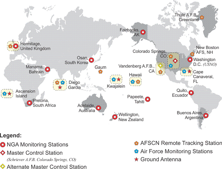
The question might arise in your mind, where does this Navigation Message and the information embedded there come from? It comes from the Control Segment. There are three segments in the GPS system: the User Segment, the Control Segment, and the Space Segment. The Space Segment is obviously the satellites themselves, the User Segment are all of us with our GPS receivers, and the Control Segment, well, here's an illustration that shows you the expanded Control Segment that is currently operational.
It's a good thing that we have the Control Segment a little bit modernized from what it once was. We'll talk more about that in the future, but here we have the stations, some of them monitor stations and then some of them actually have upload capability as well. In general, what happens is this. The GPS satellites are tracked by at least, now, three of these stations simultaneously all the time. Now, by tracking them, they are able to do several things. For example, since the stations already know their positions on the surface of the Earth, they are able to collect the signals from the satellites and know how much they have been delayed or attenuated by the atmosphere. They're also able to track the satellites and determine their path, their orbit. From this, their ephemerides can be calculated. The control station is also able to compare the signal coming from the satellite with the station's atomic clock, see the difference between the two, and then upload a clock correction to the satellite.
This is basically how the information is derived. It then goes from the tracking stations to the Master Control Station in Colorado Springs at Schriever Air Force Base, where calculations are done and the components that we've just seen in the Navigation Message are generated.
Those corrections go back to the upload stations with the ground antennas and are uploaded back to the satellites. That's where the information that is in the Navigation Message comes from. It's the control stations in the Control Segment on the surface of the Earth comparing the received signal from the satellite with their satellite clock, with their atomic clock and with their actual known position. This way, they can derive the corrections that go into the satellite's Navigation Message.
GPS Time
| local | 2020-09-09 14:37:04 | Wednesday | day 253 | timezone UTC-6 |
|---|---|---|---|---|
| UTC | 2020-09-09 20:37:04 | Wednesday | day 253 | MJD 59101.85907 |
| GPS | 2020-09-09 20:37:22 | week 2122 | 333442 s | cycle 2 week 0074 day 3 |
| Loran | 2020-09-09 20:37:31 | GRI 9940 | 47 s until | next TOC 20:37:51 UTC |
| TAI | 2020-09-09 20:37:41 | WEDNESDAY | day 253 | 37 leap seconds |
There is time-sensitive information in the NAV message in both subframe 1 and subframe 4. The information in subframe 4 helps a receiver relate two different time standards to one another. One of them is GPS Time and the other is Coordinated Universal Time (UTC).
GPS Time is the time standard of the GPS system. It is also known as GPS System Time (GPST). Coordinated Universal Time is the time standard for the world. The rates of these two standards are virtually the same. Specifically, the rate of GPS Time is kept within 1 microsecond, and usually less than 25 nanoseconds, of the rate of Coordinated Universal Time (UTC). The exact difference is in two constants, A0 and A1 in the NAV message, which give the time difference and rate of system time against UTC.
The rate of UTC itself is carefully determined. It is steered by about 65 timing laboratories and hundreds of atomic clocks around the world and is remarkable in its stability. In fact, it is more stable than the rotation of the earth itself, such that UTC and the rotation gradually get out of sync with one another. Therefore, in order to keep the discrepancy between UTC and the earth’s actual motion under 0.9 seconds, corrections of 1 second, called leap seconds, are periodically introduced into UTC. In other words, the rate of UTC is consistent and stable all the time, but the numbers denoting the moment of time changes whenever a 1-second leap second is introduced.
However, leap seconds are not used in GPS Time. It is a continuous timescale. Nevertheless, there was a moment when GPS Time was identical to UTC. It was midnight, January 6, 1980. Since then, many leap seconds have been added to UTC, but none have been added to GPS Time. So, even though their rates are virtually identical, the numbers expressing a particular instant in GPS Time are different by some seconds from the numbers expressing the same instant in UTC. For example, GPS time was 16 seconds ahead of UTC on July 1, 2012 and 18 seconds ahead of UTC on September 11, 2020
Information in subframe 4 of the NAV message includes the relationship between GPS time and UTC, and it also notes future scheduled leap seconds. In this area, subframe 4 can accommodate 8 bits, 255 leap seconds, which should suffice until about 2330. The NAV message also contains information the receiver needs to come close to correlating its clock with that of the clock on the satellite. But because the time relationships in GPS are changing constantly, they can only be partially defined in these subframes. It takes more than a portion of the NAV message to define those relationships to the necessary degree of accuracy.
The Control Segment keeps track of time and uploads clock corrections to the satellites. However, the oscillators (clocks) in satellites have a tendency to drift. They're not perfect timekeepers, and they're affected by several things, moving in and out of the shadow of the Earth, gravitational changes, and so on. These effects cause the satellite's clocks to not oscillate perfectly. Their rate can vary. Nevertheless, the Control Segment does not constantly tweak the clocks in the satellites to keep them perfectly on GPS time. They let them wander a little bit, but keep them within the limit of one millisecond of GPS Time. They find that by doing this, it keeps the clock in the satellites healthy longer. It extends their life. You will note that the first things to go on a satellite are its clocks. This is one reason that many of them have multiple oscillators.
So, the message is that the Control Segment introduces a clock correction into the Navigation Message that gives your receiver a way to correlate the drift of the oscillator(s) in the satellite with GPS time. This is one way to keep the time standard within limits.
Ephemerides

Another example of time-sensitive information is found in subframes 2 and 3 of the NAV Message. They contain information about the position of the satellite, with respect to time. This is called the satellite’s ephemeris. The ephemeris that each satellite broadcasts to the receivers provides information about its position relative to the earth. In other words, these are the coordinates of the satellite in space at the instant the Control Segment uploads the ephemerides to the Navigation Message for each individual satellite. Most particularly, it provides information about the position of the satellite antenna's phase center. The ephemeris is given in a right ascension (RA) system of coordinates. There are six orbital elements; among them are the size of the orbit, that is its semimajor axis, a, and its shape, that is the eccentricity, e. However, the orientation of the orbital plane in space is defined by other things, specifically the right ascension of its ascending node, Ω, and the inclination of its plane, i. These parameters along with the argument of the perigee, ω, and the description of the position of the satellite on the orbit, known as the true anomaly, provides all the information the user’s computer needs to calculate earth-centered, earth-fixed, World Geodetic System 1984, GPS Week 1762 (WGS84 [G1762]) coordinates of the satellite at any moment. Another example of time-sensitive information is found in subframes 2 and 3 of the Navigation message. They contain information about the position of the satellite, with respect to time. The broadcast ephemeris, however, is far from perfect. It is expressed in parameters named for the seventeenth century German astronomer Johann Kepler. The ephemerides may appear Keplerian, but in this case, the orbits of the GPS satellites deviate from nice smooth elliptical paths because they are unavoidably perturbed by gravitational and other forces. They are affected by lots of biases. Therefore, the orbits change with time so their actual paths through space are found in the result of least-squares, curve-fitting analysis. The accuracies of both the broadcast clock correction and the broadcast ephemeris deteriorate with time, so the ephemeris needs to be updated periodically to keep it within the accuracy required to get good positions on the Earth's surface. As a result, one of the most important parts of this portion of the NAV message is called IODE. IODE is an acronym that stands for Issue of Data Ephemeris, sort of a time stamp on the ephemeris that the receiver gets from the navigation message, and it appears in both subframes 2 and 3. Remember, the satellites are the control points from which the distances must be derived.
Atmospheric Correction
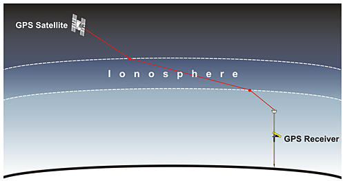
Subframe 4 addresses atmospheric correction. As with subframe 1, the data there offer only a partial solution to a problem. The Control Segment’s monitoring stations find the apparent delay of a GPS signal caused by its trip through the ionosphere through an analysis of the different propagation rates of the carrier frequencies broadcast by GPS satellites, L1, L2 and L5. These frequencies and the effects of the atmosphere on the GPS signal will be discussed later. For now, it is sufficient to say that a single-frequency receiver depends on the ionospheric correction in subframe 4 of the NAV message to help remove part of the error introduced by the atmosphere, whereas a receiver that can track more than one carrier has a bit of an advantage by comparing the differences in the frequency dependent propagation rates.
As the illustration indicates, the signal from the GPS satellite appears to slow down as it goes through the ionosphere. The atmospheric correction has been uploaded to the satellite from the Control Segment. The Control Segment can quantify the slowing because the tracking station is at a known point.
The ionosphere is dispersive. Since the GPS satellite broadcasts signals at different frequencies, it is important to understand that these frequencies are affected differently as they pass through the ionosphere. Their propagation rates are slowed differently in the ionosphere. They're not slowed at exactly the same rate. We'll talk more about that in a little bit.
For the moment, it's sufficient to say that a single frequency receiver, and there are such things, of course, a single frequency GPS receiver is somewhat handicapped by the fact that it cannot model the ionosphere. If the receiver has only one frequency to work with, it can't take advantage of the fact that it could quantify how much the signals have been affected by the ionosphere for itself, rather than relying exclusively on the Atmospheric Correction in the Navigation Message. A single frequency GPS receiver must rely almost completely on the Navigation Message Atmospheric Correction. This is a bit of a handicap. The atmosphere over Kwajalien in the Pacific might be quite different than the atmosphere above a single frequency GPS receiver in the continental US. This is one reason that the Navigation Message is not as perfect as we would like it to be.
The Almanac, Time to First Fix and Satellite Health

The Almanac
As mentioned briefly earlier, the information in the almanac in subframes 4 and 5 tells the receiver where to find all the GPS satellites. Subframe 4 contains the almanac data for satellites with pseudorandom noise (PRN) numbers from 25 through 32, and subframe 5 contains almanac data for satellites with PRN numbers from 1 through 24. The Control Segment generates and uploads a new almanac every day to each satellite, at least every six days, but typically on a daily basis.
While a GPS receiver must collect a complete ephemeris from each individual GPS satellite to know its correct orbital position, it is convenient for a receiver to be able to have some information about where all the satellites in the constellation are by reading the almanac from just one of them. The almanacs are much smaller than the ephemerides because they contain coarse orbital parameters and incomplete ephemerides, but they are still accurate enough for a receiver to generate a list of visible satellites at power-up. They, along with a stored position and time, allow a receiver to find its first satellite.
If a receiver has been in operation recently and has some leftover almanac and position data in its non-volatile memory from its last observations, it can begin its search with what is known as a warm start. A warm start is also known as a normal start. In this condition, the receiver might begin by knowing the time within about 20 seconds and its position within 100 km or so, and this approximate information helps the receiver estimate the range to satellites. For example, it will be able to restrict its search for satellites to those likely above its horizon, rather than wasting time on those below it. Limiting the range of the search decreases the time to first fix (TTFF). It can be as short as 30 seconds with a warm start.
On the other hand, if a receiver has no previous almanac or ephemeris data in its memory, it will have to perform a cold start, also known as a factory start. Without previous data to guide it, the receiver in a cold start must search for all the satellites without knowledge of its own position, velocity, or the time. When it does finally manage to acquire the signal from one, it gets some help and can begin to download an almanac. That almanac data will contain information about the approximate location of all the other satellites. The period needed to receive the full information is 12.5 minutes.
The time to first fix (TTFF) is longest at a cold start, less at warm, and least at hot. A receiver that has a current almanac, a current ephemeris, time and position can have a hot start. A hot start can take from 1/2 to 20 seconds.
Estimating how long each type of start will actually take is difficult; overhead obstructions interrupting the signal from the satellites, the GPS signals reflecting from nearby structures, etc., can delay the loading of the ephemeris necessary to lock onto the satellite's signals.
Satellite health
Subframe 1 contains information about the health of the satellite the receiver is tracking when it receives the NAV message and allows it to determine if the satellite is operating within normal parameters. Subframes 4 and 5 include health data all of the satellites, data that is periodically uploaded by the Control Segment. These subframes inform users of any satellite malfunctions before they try to use a particular signal. The codes in these bits may convey a variety of conditions. They may tell the receiver that all signals from the satellite are good and reliable, or that the receiver should not currently use the satellite because there may be tracking problems or other difficulties. They may even tell the receiver that the satellite will be out of commission in the future; perhaps it will be undergoing a scheduled orbit correction. GPS satellites' health is affected by a wide variety of breakdowns, particularly clock trouble. That is one reason they carry multiple clocks.
The almanac in sub frames four and five tell the receiver where to find the satellites. The little truncated ephemerides in the almanac help it do that. There is also information about the satellite health in the Navigation Message. GPS satellites operate in a rather hostile environment, and if they're having trouble, i.e., if some of the clocks are not operating within acceptable parameters, the health data allows the receiver to have that information. For example, a receiver might receive information that a satellite is unhealthy and shouldn't be used in the positioning.
Telemetry and Handover Words
| Subframe | 1 word | 2 words | 3-10 words |
|---|---|---|---|
| 1 | TLM | How | Clock correction, GPS week, Satellite Health, etc. |
| 2 | TLM | How | Ephemeris |
| 3 | TLM | How | Ephemeris |
| 4 | TLM | How | Ionosphere, PRN 25-32 Satellite Almanac and Health, UTC, etc. (Subframe 4 contains 25 subcommutated pages) |
| 5 | TLM | How | PRN 1-24 Satellite Almanac and Health, etc. (Subframe 5 contains 25 subcommutated pages) |
Each of these five subframes begins with the same two words: the telemetry word (TLM) and the handover word (HOW). Unlike nearly everything else in the NAV message, these two words are generated by the satellite itself. As shown in the column headed Seconds of the Week at Midnight on that Day in Table 1.1, GPS time restarts each Sunday at midnight (0:00 o’clock). These data contain the time since last restart of GPS time on the previous Sunday, 0:00 o’clock.
The TLM is the first word in each subframe. It indicates the status of uploading from the Control Segment while it is in progress and contains information about the age of the ephemeris data. It also has a constant unchanging 8-bit preamble of 10001011, and a string helps the receiver reliably find the beginning of each subframe.
The HOW provides the receiver information on the time of the GPS week (TOW) and the number of the subframe, among other things. For example, the HOW’s Z count (an internally derived 1.5 second epoch) tells the receiver exactly where the satellite stands in the generation of positioning codes.
The telemetry word indicates the status of uploading the control segment, if it's in process or not. This allows your receiver to know that.
Also, it allows you to know the beginning of each word from the data string. The handover word is useful in a couple of ways, but probably most importantly to tell your receiver where the satellite is in its broadcast of the codes. There are several codes in GPS. We will talk more about those.
The P and C/A Codes
The P and C/A codes are complicated, so complicated that they appear to be noise at first. In fact, they are known as pseudorandom noise, or PRN, codes. Actually, they are carefully designed. They have to be. They must be capable of repetition and replication. However, unlike the Navigation Message, the P and C/A codes are not vehicles for broadcasting information that has been uploaded by the Control Segment. They carry the raw data from which GPS receivers derive their time and distance measurements.

P Code
The P code is called the Precise code. It is a particular series of ones and zeroes generated at a rate of 10.23 million bits per second. It is carried on both L1 and L2, and it is very long, 37 weeks (2x1014 bits in code). Each GPS satellite is assigned a part of the P code all its own, and then repeats its portion every 7 days. This assignment of one particular week of the 37-week-long P code to each satellite helps a GPS receiver distinguish one satellite’s transmission from another. For example, if a satellite is broadcasting the fourteenth week of the P code, it must be Space Vehicle 14 (SV 14). The encrypted P code is called the P(Y) code.
There is a flag in subframe 4 of the NAV message that tells a receiver when the P code is encrypted into the P(Y) code. This security system has been activated by the Control Segment since January 1994. It is done to prevent spoofing. Spoofing is generation of false transmissions masquerading as the Precise Code. This countermeasure called Antispoofing (AS) is accomplished by the modulation of a W-Code to generate the more secure Y-Code that replaces the P code. Commercial GPS receiver manufacturers are not authorized to use the P(Y) code directly. Therefore, most have developed proprietary techniques both for carrier wave and pseudorange measurements on L2 indirectly. There is now a civilian code on L2 (L2C). There is also now a military code known as the M code. We will discuss both of these later.
The Navigation Message can be thought of as the NAV Code, but there are others. Positioning, one of the primary objectives of GPS, is really the office of the P-Code, the C/A Code and some others that are newer than these legacy codes. The P code is the Precise code, The C/A code is the Civilian Access code. They're modulated onto carrier waves. For example, when you listen to a radio in your car and the announcer says you're listening to, let's say, 760 megahertz... well, of course, you're not listening to 760 megahertz. You can't hear that. Human hearing tops out at about 0.02 megahertz. What you hear is the modulation of speech and music onto the 760 megahertz carrier. The same idea is used in GPS. But with a radio, of course, the modulation is typically a frequency modulation or an amplitude modulation for FM and AM, respectively. In GPS, the modulation is done differently. Phase modulation is used. The image here is intending to show that. The P code in the image is a sine wave. It has particularly sharp peaks, but it is still a sine wave. Please note that up at the top of the blue line, there's a sequence of 1's and 0's. These indicate code chips of a binary code.
Please notice the way these code chips transition from 1 to 0 and back to 1. At those instances the sine wave, the blue line, does not go all the way to the top or bottom. When there is a transition from a 1 to a 0 or from a 0 to a 1, the blue line stops in the middle and reverses direction. However, when the code chip just goes from a 1 to a 1, or from a 0 to a 0, there is no interruption of the normal sine wave path. In those cases, the blue line does go all the way up to the top, and it goes all the way down to the bottom.
This technique is called phase modulation.
The C/A Code
The C/A code is also a particular series of ones and zeroes, but the rate at which it is generated is 10 times slower than the P(Y) code. The C/A code rate is 1.023 million bits per second. Here, satellite identification is quite straightforward. Not only does each GPS satellite broadcast its own completely unique 1023 bit C/A code, it repeats its C/A code every millisecond. The legacy C/A code is broadcast on L1 only. It used to be the only civilian GPS code, but no longer; it has been joined by a new civilian signal known as L2C that is carried on L2.

SPS and PPS
Still, the C/A code is the vehicle for the Standard Positioning Service, SPS, which is used for most civilian surveying applications. The P(Y) code on the other hand provides the same service for the precise positioning servicer, PPS. The idea of SPS and PPS was developed by the Department of Defense many years ago. SPS was designed to provide a minimum level of positioning capability considered consistent with national security, ±100m, 95% of the time, when intentionally degraded through Selective Availability (SA).
Selective Availability, the intentional dithering of the satellite clocks by the Department of Defense was instituted in 1989, because the accuracy of the C/A point positioning as originally rolled out was too good! As mentioned above, the accuracy was supposed to be ±100 meters horizontally, 95% of the time, with a vertical accuracy of about ±175 meters. But, in fact, it turned out that the C/A-code point positioning gave civilians access to accuracy of about ±20 meters to ±40 meters. That was not according to plan, so the satellite clocks’ accuracy was degraded on the C/A code. The good news is that the intentional error source called SA is gone. It was switched off on May 2, 2000 by presidential order. The intentional degradation of the satellite clocks is a thing of the past. Actually, Selective Availability never did hinder the surveying applications of GPS. We will delve into the reason a bit later. In any case, satellite clock errors, the unintentional kind, still contribute error to GPS positioning.
PPS is designed for higher positioning accuracy and was originally available only to users authorized by the Department of Defense; that has changed somewhat, more about that later in this chapter. It used to be that the P(Y) code was the only military code. That is no longer the case. It has been joined by a new military signal called the M-code.
The C/A Code or Civilian Acquisition or Access Code is generated 10 times slower than the P-Code. The GPS fundamental clock rate is 10.23 megahertz, but C/A Code is generated at 1.023 megabits per second.
The C/A Code is modulated onto the carrier by phase modulation, too.
The image shows a green line, a sine wave that only transitions when it reaches that center line and reverses direction. That is a phase shift, and then the code, it goes from the 1 to the 0 or from the 0 to the 1.
Modulation of Carrier Wave

All the codes mentioned come to a GPS receiver on a modulated carrier; therefore, it is important to understand how a modulated carrier is generated. The signal created by an electronic distance measuring (EDM) device in a total station is a good example of a modulated carrier.
EDM Ranging
Distance measurement in modern surveying is done electronically. Distance is measured as a function of the speed of light, an electromagnetic signal of stable frequency and elapsed time. Frequencies generated within an electronic distance measuring device (EDM) can be used to determine the elapsed travel time of its signal, because the signal bounces off a reflector (aka corner cube) and returns to where it started. An EDM only needs one oscillator at the point of origin, because its electromagnetic wave travels to a retroprism and is reflected back to its origination. It is a two-way system, but the EDM is both the transmitter and the receiver of the signal. On the signal's return, the EDM can analyze it and determine the distance. In general terms, the instrument can take half the time elapsed between the moment of transmission and the moment of reception, multiply by the speed of light, and find the distance between itself and the retroprism (Distance = Elapsed Time x Rate).
The fundamental elements of the calculation of the distance measured by an EDM, ρ, are the time elapsed between transmission and reception of the signal, Δt, and the speed of light, c.
Distance = ρ
Elapsed Time = Δt
Rate = c
GPS Ranging

The one-way ranging used in GPS is more complicated. The broadcast signals from the satellites are collected by the receiver, not reflected. Nevertheless, the same measurement concept is used. In general terms, the full time elapsed between the instant a GPS signal leaves a satellite and arrives at a receiver, multiplied by the speed of light, is the distance between them. Unlike the wave generated by an EDM, a GPS signal cannot be analyzed at its point of origin. The measurement of the elapsed time between the signal’s transmission by the satellite and its arrival at the receiver requires two clocks (aka oscillators), one in the satellite and one in the receiver. This complication is compounded because these two clocks would need to be perfectly synchronized with one another to calculate the elapsed time, and hence the distance, between them exactly. Since such perfect synchronization is impossible, the problem is addressed mathematically.
In the image, the basis of the calculation of a range measured from a GPS receiver to the satellite, ρ, is the multiplication of the time elapsed between a signal’s transmission and reception, Δt, by the speed of light, c. A discrepancy of 1 microsecond, 1 millionth of a second, from perfect synchronization, between the clock aboard the GPS satellite and the clock in the receiver can create a range error of 299.79 meters, far beyond the acceptable limits for nearly all surveying work.
So, since perfect synchronization is not in the cards, we have to solve for time.
Phase Angles

Here's a sine wave illustrating a single wavelength of 1 Hertz, that is a wavelength that takes 1 second to cycle through 360 degrees. The 0°, 90°, 180°, 270° and 360° are known as phase angles. They are important to the modulation of the carrier by phase and that is the method of attaching the codes to the GPS carriers.
The time measurement devices used in both EDM and GPS measurements are clocks only in the most general sense. They are more correctly called oscillators, or frequency standards. In other words, rather than producing a steady series of ticks, they keep time by chopping a continuous beam of electromagnetic energy at extremely regular intervals. The result is a steady series of wavelengths and the foundation of the modulated carrier. As long as the rate of an oscillator’s operation is very stable, both the length and elapsed time between the beginning and end of every wavelength of the modulation will be the same. Therefore, the phase angles will also occur at definite and constant distances.
Phase Shift

Phase Shift
The image shows again the EDM sending out the transmitted wave in blue, with the phase angles indicated as before. The signal goes to the retro prism and returns. When it returns, shown in the dashed red line, notice the phase angles. It is clear that the return signal does not come back exactly in phase with the transmitted wave. In other words, the phase angles on the reflected wave do not match those on the transmitted wave. The key element here is that the EDM generates another wave that is exactly the same as the wave it transmitted. However, it keeps the additional wave (the blue one) at home so that when the reflected wave returns, it can be compared with it. By comparing the returned wave—the one here in the dashed red line—with the exact replica of the transmitted wave, the EDM can determine how much the returned wave is phase shifted, that is out of phase, with the original transmitted wave.
Since all measurements will not neatly fit complete wavelengths, the EDM finds the fractional part of its measurement electronically. It does a comparison. It compares the phase angle of the returning signal to that of a replica of the transmitted signal that it keeps inside to determine the phase shift. That phase shift represents the fractional part of the measurement.
How does it work? First, it is important to remember that points on a modulated carrier are defined by phase angles, such as 0°, 90°, 180°, 270° and 360°. When two modulated carrier waves reach exactly the same phase angle at exactly the same time, they are said to be in phase, coherent, or phase locked. However, when two waves reach a phase angle at different times, they are out of phase or phase shifted. For example, in the image, the sine wave shown by the dashed red line has returned to an EDM from a reflector. Compared with the sine wave shown by the solid blue line, it is out of phase by one-quarter of a wavelength. The distance between the EDM and the reflector, ρ, is then:
where:
N = the number of full wavelengths the modulated carrier has completed
d = the fractional part of a wavelength at the end that completes the doubled distance.
In this example, d is three-quarters of a wavelength because it lacks its last quarter.
Both EDM and GPS ranging use the method represented in this illustration. In GPS, the measurement of the difference in the phase of the incoming signal and the phase of the internal oscillator in the receiver reveals the small distance at the end of a range. In GPS, the process is called carrier phase ranging, as the name implies, the observable is the carrier wave itself in that case.
The Integer Ambiguity Problem

Both EDM and GPS ranging use the method represented in this illustration. In GPS, the measurement of the difference in the phase of the incoming signal and the phase of the internal oscillator in the receiver reveals the small distance at the end of a range.
By comparing the phase of the signal returned from the reflector with the reference wave it kept at home, an EDM can measure how much the two are out of phase with one another. However, this measurement can only be used to calculate a small part of the overall distance. It only discloses the length of a fractional part of a wavelength used. This leaves a big unknown, namely the number of full wavelengths of the EDM’s modulated carrier between the transmitter and the receiver at the instant of the measurement. This cycle ambiguity is symbolized by N. Fortunately, the cycle ambiguity can be solved in the EDM measurement process. The key is using carriers with progressively longer wavelengths. For example, the submeter portion of the overall distance can be resolved using a carrier with the wavelength of a meter. This can be followed by a carrier with a wavelength of 10 meters, which provides the basis for resolving the meter aspect of a measured distance. This procedure may be followed by the resolution of the tens of meters using a wavelength of 100 meters. The hundreds of meters can then be resolved with a wavelength of 1000 meters, and so on.
Here is that comparison, the reference wave in blue with the reflected wave with the dashed red line. The reflected wave came back out of phase by a quarter of a wavelength. With an EDM, wavelengths of varying length can be sent out. For example, if the EDM sends out a wavelength of 100 meters, then by looking at the fractional part of that 100-meter wavelength, it would be possible to determine the tens of meters in the distance. The hundreds of meters of the overall distance could be resolved by sending out a wavelength of 1,000 meters and looking at the fractional part (by phase comparison). This method depends on the fact that the EDM survey can send out waves of different wavelengths and have them return to where they came from. That makes comparison of the returned wave with the reference wave possible. By comparing phase angles, the fractional part of the wavelength that went out can be determined. The components of the total distance are built up by sending on wavelengths of different size; first the thousands of feet, then the hundreds of feet, then the single feet, and finally the decimals of feet. However, this whole method is not possible in GPS surveying. There are only three carriers; L1, L2, and L5. They have constant wavelengths. Therefore, while it's possible to determine the fractional part of the wavelength, that one small component of the distance, from a single measurement, knowing the number of full wavelengths between the receiver and satellite is more difficult. This is known as the integer ambiguity problem.
A Different Strategy


Unlike an EDM measurement, the wavelengths of GPS carriers cannot be periodically changed to resolve the cycle ambiguity problem. GPS needs a different strategy. The satellites broadcast only three carriers, L1, L2 and L5. They have constant wavelengths and only propagate from the satellites to the receivers, one direction. Still, the carrier phase measurements remain an important observable in GPS ranging.
Two Types of Observables


The word observable is used throughout GPS literature to indicate the signals whose measurement yields the range or distance between the satellite and the receiver. The word is used to draw a distinction between the thing being measured, "the observable" and the measurement, "the observation." In GPS, there are two types of observables. The codes are one type of observable. We've talked about how that is modulated onto the carrier. There's another type of observable. That's the carrier itself without the codes. The carrier is the basis of the techniques used for high-precision GPS surveys. In the upper image, you see the pseudorange code observable illustrated as square waves of code states, and in the lower image, you see the carrier wave observable, which is just a constant sine wave, not modulated. The code solution provides a pseudorange. The pseudorange can serve applications when virtually instantaneous point positions are required or relatively low accuracy will suffice. These basic observables can also be combined in various ways to generate additional measurements that have certain advantages. It is in this latter context that pseudoranges are used in many GPS receivers as a preliminary step toward the final determination of position by a carrier phase measurement. Many GPS receivers use the pseudorange code observable as sort of the front door, a way to begin the determination of a position, and then, frequently, they switch to the carrier to refine that position. The foundation of pseudoranges is the correlation of code carried on a modulated carrier wave received from a GPS satellite with a replica of that same code generated in the receiver. Most of the GPS receivers used for surveying applications are capable of code correlation. That is, they can determine pseudoranges. These same receivers are usually capable of determining ranges using the unmodulated carrier, as well. However, first let us concentrate on the pseudorange.
Spread Spectrum and Code Modulation of L1 GPS Carrier

A carrier wave can be modulated in various ways. Radio stations use modulated carrier waves. The radio signals are AM, amplitude modulated or FM, frequency modulated. When your radio is tuned to 105 FM, you are not actually listening to 105 MHz; despite the announcer’s assurances, it is well above the range of human hearing. 105 MHz is just the frequency of the carrier wave that is being modulated. It is those modulations that occur that make the speech and music intelligible. They come to you at a much slower frequency than does the carrier wave. The GPS carriers L1, L2, and L5 could have been modulated in a variety of ways to carry the binary codes, the 0s and 1s, that are the codes. Neither amplitude nor frequency modulation are used in GPS. It is the alteration of the phases of the carrier waves that encodes them. It is phase modulation that allows them to carry the codes from the satellites to the receivers. One consequence of this method of modulation is that the signal can occupy a broader bandwidth than would otherwise be possible. The GPS signal is said to have a spread spectrum because of its intentionally increased bandwidth. In other words, the overall bandwidth of the GPS signal is much wider than the bandwidth of the information it is carrying. In other words, while L1 is centered on 1575.42 MHz, L2 is centered on 1227.60 MHz, and L5 on 1176.45 MHz, but the width of these signals takes up a good deal more space on each side of these frequencies than might be expected. For example, the C/A code signal is spread over a width of 2.046 MHz or so, the P(Y) code signal is spread over a width about 20.46 MHz on L1 and the coming L1C signal will be spread over 4.092 MHz as shown in the image above.
This characteristic offers several advantages. It affords better signal to noise ratio, more accurate ranging, less interference, and increased security. However, spreading the spectral density of the signal also reduces its power. The weakness of the signal makes it difficult to receive undercover.

In any case, the most commonly used spread spectrum modulation technique is known as binary phase shift keying (BPSK). This is the technique used to create the NAV Message, the P(Y) code and the C/A code. The binary biphase modulation is the switching from 0 to 1 and from 1 to 0 accomplished by phase changes of 180º in the carrier wave. Put another way, at the moments when the value of the code must change from 0 to 1, or from 1 to 0, the change is accomplished by an instantaneous reverse of the phase of the carrier wave. It is flipped 180º. And each one of these flips occurs when the phase of the carrier is at the zero-crossing (the gray centerline inthe middle of the sine wave illustrations above). Each 0 and 1 of the binary code is known as a code chip. 0 represents the normal state, and 1 represents the mirror image state.
The rate of all of the components of GPS signals are multiples of the standard rate of the oscillators. The standard rate is 10.23 MHz. It is known as the fundamental clock rate and is symbolized Fo For example, the GPS carriers are 154 times Fo, or 1575.42 MHz, 120 times Fo, or 1227.60 MHZ, and 115 times Fo, or 1176.45 MHZ. These represent L1, L2, and L5 respectively. The codes are also based on Fo. 10.23 code chips of the P(Y) code, 0s or 1s, occur every microsecond. In other words, the chipping rate of the P(Y) code is 10.23 million bits per second (Mbps), exactly the same as Fo, 10.23 MHZ. The chipping rate of the C/A code is 10 times slower than the P(Y) code. It is one tenth of Fo, 1.023 Mbps. Ten P(Y) code chips occur in the time it takes to generate one C/A code chip. This is a reason why a P(Y) code derived pseudorange is more precise than a C/A code pseudorange.
More About Code Chips
Up at the top is the C/A Code in the green and the P-Code is in the blue below it. There are several pieces of information here. One of the things you might notice right away is the red square wave from 1 to 0 and 0 to 1 indicated down at the bottom.
For each 180-degree phase shift, there's this shift from the 1 to the 0 and back to 1, and this is represented by this red square wave. See that the C/A Code is also represented by the dashed black square wave that is turned 90 degrees or in quadrature to the P-Code.
If there were no shift in the phase of the carriers, they would not be modulated and would not be carrying the codes.
The codes chipping rates are shown on the right-hand side. Please notice that the C/A Code chipping rate is 10 times slower than the P-Code.
L1 is broadcast at 1575.42 megahertz. Its rate is a multiple of the fundamental clock rate of 10.23 megahertz.
The length of a C/A Code is 960 feet, whereas, the length of a P-Code, 10 times shorter, because the P-Code is 10 times faster, is 96 feet, and also notice the repetition period. You see here, also, the 10 P-Codes per each C/A Code chip, which is exactly as you would expect.
The C/A Code is repeated very quickly; whereas the P-Code does not repeat for seven days, making it more secure as would be expected with a classified precise code.
Code Correlation

Strictly speaking, a pseudorange observable is based on a time shift. This time shift can be symbolized by dτ, d tau, and is the time elapsed between the instant a GPS signal leaves a satellite and the instant it arrives at a receiver. The concept can be illustrated by the process of setting a watch from a time signal heard over a telephone.
Propagation Delay
Imagine that a recorded voice said, “The time at the tone is 3 hours and 59 minutes.” If a watch was set at the instant the tone was heard, the watch would be wrong. Supposing that the moment the tone was broadcast was indeed 3 hours and 59 minutes, the moment the tone is heard must be a bit later. It is later because it includes the time it took the tone to travel through the telephone lines from the point of broadcast to the point of reception. This elapsed time would be approximately equal to the length of the circuitry traveled by the tone divided by the speed of the electricity, which is the same as the speed of all electromagnetic energy, including light and radio signals. In fact, it is possible to imagine measuring the actual length of that circuitry by doing the division.
In GPS, that elapsed time is known as the propagation delay, and it is used to measure length. The measurement is accomplished by a combination of codes. The idea is somewhat similar to the strategy used in EDMs. But where an EDM generates an internal replica of its carrier wave to correlate with the signal it receives by reflection, a pseudorange is measured by a GPS receiver using a replica of a portion of the code that is modulated onto the carrier wave. The GPS receiver generates this replica itself and it is used to compare with the code that is coming in from the satellite.
Code Correlation
To conceptualize the process, one can imagine two codes generated at precisely the same time and identical in every regard: one in the satellite and one in the receiver. The satellite sends its code to the receiver but, on its arrival, the codes do not line up even though they are identical. They do not correlate, that is, until the replica code in the receiver is time shifted a little bit. Once that is done, the receiver generated replica code fits the received satellite code. It is this time shift that reveals the propagation delay. The propagation delay is the time it took the signal to make the trip from the satellite to the receiver, dτ. It is the same idea described above as the time it took the tone to travel through the telephone lines, except the GPS code is traveling through space and atmosphere. Once the time shift of the replica code is accomplished, the two codes match perfectly and the time the satellite signal spends in transit has been measured, well, almost. It would be wonderful if that time shift could simply be divided by the speed of light and yield the true distance between the satellite and the receiver at that instant, and it is close, but there are physical limitations on the process that prevent such a perfect relationship.
Autocorrelation
As mentioned earlier, the almanac information from the NAV message of the first satellite a GPS receiver acquires tells it which satellites can be expected to come into view. With this information, the receiver can load up pieces of the C/A codes for each of those satellites. Then the receiver tries to line up the replica C/A codes with the signals it is actually receiving from the satellites. Actually lining up the code from the satellite with the replica in the GPS receiver is called autocorrelation, and depends on the transformation of code chips into code states. The formula used to derive code states (+1 and -1) from code chips (0 and 1) is:
code state = 1-2x
where x is the code chip value. For example, a normal code state is +1, and corresponds to a code chip value of 0. A mirror code state is -1, and corresponds to a code chip value of 1.
The function of these code states can be illustrated by asking three questions: First, if a tracking loop of code states generated in a receiver does not match code states received from the satellite, how does the receiver know? In that case, for example, the sum of the products of each of the receiver’s 10 code states, with each of the code states from the satellite, when divided by 10, does not equal 1. In the example in the illustration, the result is 0.40. Second, what does the receiver do when the code states in the receiver do not match the code states received from the satellite? It shifts the frequency of its search a little bit from the center of the L1 1575.42 MHZ. This is done to accommodate the inevitable Doppler shift of the incoming signal, since the satellite is always either moving toward or away from the receiver. The receiver also shifts its piece of code in time. These iterative small shifts in both time and frequency continue until the receiver code states do in fact match the signal from the satellite. Third, how does the receiver know when a tracking loop of replica code states does match code states from the satellite? In the case illustrated in the image, the sum of the products of each code state of the receiver’s replica 10, with each of the 10 from the satellite, divided by 10, is exactly 1. This is shown in the illustration at "Correlation!" where the receiver’s replica code fits the code from the satellite like a key fits a lock.
The interesting thing is that that time shift for correlation gives the receiver approximately the amount of elapsed time that it took the signal to come from the satellite to the receiver. Obviously, if the receiver knows the elapsed time, and it knows the frequency of the signal, it then knows the distance (the range) between itself and the satellite. This is how the pseudorange works. If this were the whole story, we'd be done, and of course, it isn't the whole story.
The Delay Lock Loop

Once correlation of the two codes is achieved with a delay lock loop (DLL), it is maintained by a correlation channel within the GPS receiver, and the receiver is sometimes said to have achieved lock or to be locked on to the satellites. The receiver can continue to log the signal from the satellite and stay correlated unless it is somehow interrupted by a cycle slip or an obstruction. If that happens, the receiver is said to have lost lock. However, as long as the lock is present, the NAV message is available to the receiver. Remember that one of its elements is the broadcast clock correction that relates the satellite's on board clock to GPS time, and a limitation of the pseudorange process comes up.
Imperfect Oscillators and Clock Corrections

One reason the time shift, dτ (d tau), found in autocorrelation cannot quite reveal the true range, ρ, of the satellite at a particular instant is the lack of perfect synchronization between the clock in the satellite and the clock in the receiver. Recall that the two compared codes are generated directly from the fundamental rate, Fo, of those clocks. And since these widely separated clocks, one on Earth and one in space, cannot be in perfect lockstep with one another, the codes they generate cannot be in perfect sync either. Therefore, a part of the observed time shift, dτ (d tau), must always include the disagreement between these two clocks. In other words, the time shift not only contains the signal’s transit time from the satellite to the receiver, it contains clock errors, and other errors too. In fact, whenever satellite clocks and receiver clocks are checked against the carefully controlled GPS time, they are found to be drifting a bit. Their oscillators are imperfect. It is not surprising that they are not quite as stable as the atomic clocks around the world that are used to define the rate of GPS time. They are subject to the destabilizing effects of temperature, acceleration, radiation, and other inconsistencies. In other words, clock offsets bias every satellite to receiver pseudorange observable. The difference between the satellite clock's time and GPS time is shown in dt (d small t) in the illustration. The difference in the receiver's clock from GPS time is shown in dT (d capital T) in the illustration. While the pseudorange observable shown here in dτ (d tau) is intended to be the amount of time that it took the signal to reach the receiver from the satellite, there are some difficulties. Among them are the fact that the receiver's clock is probably a quartz oscillator, and it's not terribly stable, and the clock correction in the Navigation Message which was uploaded some time before it is received isn't exactly right either. Such discrepancies are important when a nanosecond, a billionth of a second, is approximately a foot. Therefore, the pseudorange has some errors that are difficult to remove. The pseudorange, by itself, while it has the virtue of being approximately correct, is certainly not at the level of accuracy that we have come to expect from GPS. That is one reason it is called a pseudorange (i.e. false range)
The Pseudorange Equation

Clock offsets are only one of the errors in pseudoranges. Please note that the pseudorange, p, and the true range, ρ, cannot be made equivalent without consideration of clock offsets, atmospheric effects and other biases that are inevitably present.
Some of those errors are shown in this equation. On the left-hand side, the pseudorange measurement equals rho, the true range, plus all of these other factors. If it were correct initially, if the pseudorange was good and complete by itself, these other factors would not need to be considered. The pseudorange, p, would be equal to the true range, rho. But, in fact, there are satellite orbital errors because the orbits of the satellites are affected by many factors including the variations in gravity, drag, and tidal forces from the sun, the moon, etc. The speed of light is constant in a vacuum, but it has to be multiplied times the satellite clock offset from GPS time minus the receiver clock offset from GPS time, because of propagation delay and imperfect oscillators among other things. While the satellite clock offset from GPS time is somewhat known from the Navigation Message, it's not perfectly known. The receiver clock offset from GPS time is not well known at all. Then, there is the ionospheric delay to be considered. There's also a bit of tropospheric delay. The troposphere includes the atmospheric layers below the ionosphere.
Then, on top of that, there's something known as multipath. Multipath means that the signal from the GPS satellite bounces off of something before it gets into the receiver. Obviously, if you're measuring distances to determine your position, that bounce creates a difficulty. There is receiver noise as a bias in the system. This is like the static that can appear on your car radio.
In short, all these biases contaminate the pseudorange position. So, while the pseudorange is a good way to get started with a GPS position, it isn't the full answer.
The One-percent Rule of Thumb

Here is convenient approximation. The maximum resolution available in a pseudorange is about 1 percent of the chipping rate of the code used. It offers a basis to evaluate pseudoranging in general and compare the potentials of P(Y) code and C/A code pseudoranging in particular. A P(Y) code chip occurs every 0.0978 of a microsecond. In other words, there is a P(Y) code chip about every tenth of a microsecond. That’s one code chip every 100 nanoseconds. Therefore, a P(Y) code based measurement can have a maximum precision of about 1 percent of 100 nanoseconds, or 1 nanosecond. What is the length of 1 nanosecond? Well, multiplied by the speed of light, it's approximately 30 centimeters, or about a foot. So, just about the very best you can do with a P(Y) pseudorange is a foot or so. Because its chipping rate is 10 times slower, the C/A code based pseudorange is 10 times less precise. Therefore, one percent of the length of a C/A code chip is 10 times 30 centimeters, or 3 meters. Using the rule of thumb, the resolution of a C/A code pseudorange is nearly 10 feet.
You might ask, at this point, if the pseudorange isn't the full answer, then how do we get the extraordinary accuracies that we depend upon GPS to produce?
The Carrier Phase Observable
This same 1 percent rule of thumb can illustrate the increased precision of the carrier phase observable over the pseudorange. First, the length of a single wavelength of each carrier is calculated using this formula
where:
= the length of each complete wavelength in meters;
= the speed of light corrected for atmospheric effects;
= the frequency in hertz.
L1 – 1575.42 MHz carrier transmitted by GPS satellites has a wavelength of approximately 19 cm
L2 – 1227.60 MHz carrier transmitted by GPS satellites has a wavelength of approximately 24 cm
The resolution available from a signal is approximately 1% of its wavelength. 1% of these wavelengths is approximately 2mm.
Carrier phase observations are certainly the preferred method for the higher precision work most have come to expect from GPS.
Discussion
Discussion Instructions
To begin the discussion sparked by the material in this lesson, I would like to pose this question:
There are both similarities and differences between a GPS carrier phase observation and a distance measurement by an EDM. Can you describe a few of each?
To participate in the discussion, please go to the Lesson 1 Discussion Forum in Canvas. (That forum can be accessed at any time by going to the GEOG 862 course in Canvas and then looking inside the Lesson 1 module.)
Summary
Now that you have some ideas about how the GPS signal carries information from the satellites to the receivers, you can delve into the errors that affect that information. The complete carrier phase observable equation can be stated as:
On the left side of the equation is the complete raw range measurement from the satellite to the receiver. On the right side is the correct range between the two and several errors known as biases.
The next lesson will give you an idea of both the origins and magnitudes of those biases.
Before you go on to Lesson 2, double-check the Lesson 1 Checklist to make sure you have completed all of the activities listed there.
Lesson 2: Biases and Solutions
The links below provide an outline of the material for this lesson. Be sure to carefully read through the entire lesson before returning to Canvas to submit your assignments.
Lesson 2 Overview
Overview
Biases are fascinating. The frequency standards, the clocks in GPS satellites, run faster than the clocks in GPS receivers, and the clocks in the GPS receivers are much less sophisticated than the clocks in the satellites. During the trip through the ionosphere, the information on the GPS signal appears to slow, and the ionosphere affects L2 more than L1. You might find it interesting that when a GPS signal reflects off a surface before it reaches your receiver, this is called multipath, and, believe it or not, it actually has something in common with a billiard ball (as a billiard ball often bounces off several surfaces before finding its way to the pocket). In this lesson, we will also talk about how GPS surveying is done.
Objectives
At the successful completion of this lesson, students should be able to:
- demonstrate biases and solutions;
- explain the error budget;
- explain the biases in the observation equations;
- describe user equivalent range error;
- identify the satellite clock bias, dt;
- define the ionospheric effect, dion;
- recognize the receiver clock bias, dT;
- describe the orbital bias;
- explain the tropospheric effect, dtrop ;
- identify multipath;
- recognize differencing;
- differentiate between classifications of positioning solutions;
- discuss relative and autonomous positioning; and
- recognize the benefits of single, double, and triple differencing.
Questions?
If you have any questions now or at any point during this week, please feel free to post them to the Lesson 2 Discussion Forum. (To access the forum, return to Canvas and navigate to the Lesson 2 Discussion Forum in the Lesson 2 module.) While you are there, feel free to post your own responses if you, too, are able to help out a classmate.
Checklist
Lesson 2 is one week in length. (See the Calendar in Canvas for specific due dates.) To finish this lesson, you must complete the activities listed below. You may find it useful to print this page out first so that you can follow along with the directions.
| Step | Activity | Access/Directions |
|---|---|---|
| 1 | Read the lesson Overview and Checklist. | You are in the Lesson 2 online content now. The Lesson 2 overview page is previous to this page, and you are on the Checklist page right now. |
| 2 | Read Chapter 2 in GPS for Land Surveyors. | Text |
| 3 | Read the lecture material for this lesson. | You are currently on the Checklist page. Click on the links at the bottom of the page to continue to the next page, to return to the previous page, or to go to the top of the lesson. You can also navigate the lecture material via the links in the Lessons menu. |
| 4 | Participate in the Discussion. | To participate in the discussion, please go to the Lesson 2 Discussion Forum in Canvas. (That forum can be accessed at any time by going to the GEOG 862 course in Canvas and then looking inside the Lesson 2 module.) |
| 5 | Prepare a 2,400 word paper on one topic covered in Lessons 1 and 2. Write on any topic that we have covered and relate it to the work you are doing now or the work you hope to do. | Please submit your paper to the Lesson 2 Basic GPS Paper Drop Box located in the Lesson 2 module in Canvas. View Calendar in Canvas for due date. |
| 6 | Read lesson Summary. | You are in the Lesson 2 online content now. The lesson Summary is the final page of the lesson. |
The Error Budget
The understanding and management of errors is indispensable for finding the true geometric range ρ between a satellite and a receiver from either a pseudorange or carrier phase observation.
Both equations include environmental and physical limitations called range biases.
Atmospheric errors are among the biases; two are the ionospheric effect, dion, and the tropospheric effect, dtrop. Other biases, clock errors symbolized by (dt-dT) and receiver noise, ερ and εφ, multipath, εmρ and εmφ, and orbital errors, dρ, are unique to satellite surveying methods. As you can see, each of these biases comes from a different source. They are each independent of one another, but they combine to obscure the true geometric range. The objective here is to discuss each of them separately.
Here, we see the formula of the pseudorange error budget on the upper portion. As it indicates, p is the pseudorange, measurement equals ρ, rho, the true range between the GPS receiver and satellite. However, as you can see, there are many more elements, errors, or biases that contaminate the pseudorange— the satellite orbital errors, the ephemeris errors, etc.
The time difference (dt-dT) is between the satellite clock offset, and the receiver clock offset from GPS Time, as was mentioned in the previous lesson. There is also the ionospheric delay, the attenuation, of the signal as it passes through the ionosphere. Distinct from these biases are multipath and receiver noise. These two are distinct because, unlike the others, it is difficult to deal with them in a statistical way. Nevertheless, all are part of the error budget.
Directly below the pseudorange formula, you see the carrier phase formula. It also equals true range symbolized by capital phi,Φ. It includes errors that are very similar to those in the pseudorange formula. But one is included that is obviously different. It is symbolized by the capital N followed by the letter lambda, λ. This is the integer ambiguity. It doesn't occur in the pseudorange measurement.
The management of the errors shown in the formulas, the biases, is indispensable for finding the true range from either a pseudorange or a carrier phase observation. In this lesson, we're going to try to understand the source of these errors so that they can be dealt with.
User Equivalent Range Error

The summary of the total error budget affecting a pseudorange from the user's point of view is called the user equivalent range error, UERE. This expression, often used in satellite surveying literature, is the square root of the sum of the squares of the individual biases. See figure above. The UERE is the ranging error between a satellite and the user’s receiver. It can be shown as a distance that includes both the signal in space ranging error called URE (User Range Error) and the user equipment error (UEE).
Some of the biases that make up the UERE such as those attributable to the atmosphere dion , dtrop and satellite orbits dρ increase and decrease with the length of the baselines between receivers. Differential correction techniques can often limit the effect of these errors. Others included in the UERE, such as those due to receiver noise, ερ and εφ, multipath, εmρ and εmφ, do not increase and decrease with the length of the baselines between receivers.
The Satellite Clock
The Satellite Clock Bias, dt

One of the largest errors can be attributed to the satellite clock bias. It can be quite large, especially if the broadcast clock correction is not used by the receiver to bring the time signal acquired from a satellite’s onboard clock in line with GPS time. As time is a critical component in the functioning of GPS, it is important to look closely at the principles behind this bias.
The onboard satellite clocks are independent of one another. While GPS time itself is designed to be kept within one microsecond, 1 µsec or one-millionth of a second, of UTC, excepting leap seconds, the satellite clocks can be allowed to drift up to a millisecond, 1 msec or one-thousandth of a second, from GPS time. They are allowed to drift within this tolerance because the Control Segment doesn't want to constantly tweak the clocks, as this would cause the clocks to deteriorate more rapidly. Although the GPS satellites have been robust, I think it's fair to say that the clocks are one of their more fragile components. Instead, we have the broadcast clock correction in the Navigation Message. This is the correction that the Control Segment provides to the receiver to use to bring the satellite clock in line with GPS time.
Relativistic Effects on the Satellite Clock
Albert Einstein’s special and general theories of relativity apply to the clocks involved here. At 3.874 kilometers per second, the clocks in the GPS satellites are traveling at great speed, and that makes the clocks on the satellites appear to run slower than the clocks on earth by about 7 microseconds a day. However, this apparent slowing of the clocks in orbit is counteracted by the weaker gravity around them. The weakness of gravity makes the clocks in the satellites appear to run faster than the clocks on earth by about 45 microseconds a day. Therefore, on balance, the clocks in the GPS satellites in space appear to run faster by about 38 microseconds a day than the clocks in GPS receivers on earth. So, to ensure the clocks in the satellites will actually produce the correct fundamental frequency of 10.23 MHz in space, their frequencies are set to 10.22999999543 MHz before they are launched into space.
There is yet another consideration, the eccentricity of the orbit of GPS satellites. With an eccentricity of 0.02, this effect on the clocks can be as much as 45.8 nanoseconds. Fortunately, the offset is eliminated by a calculation in the GPS receiver itself; thereby avoiding what could be ranging errors of about 14 meters. The receiver is moving, too, of course, so an account must be made for the motion of the receiver due to the rotation of the earth during the time it takes the satellite's signal to reach it. This is known as the Sagnac effect, and it is 133 nanoseconds at its maximum. Luckily, these relativistic effects can be accurately computed and removed from the system.

The Ionospheric Effect
The Ionospheric Effect, dion
The Earth's Ionosphere is variable

One of the largest errors in GPS positioning is attributable to the atmosphere. The long, relatively unhindered travel of the GPS signal through the virtual vacuum of space changes as it passes through the earth’s atmosphere. Through both refraction and diffraction, the atmosphere alters the apparent speed and, to a lesser extent, the direction of the signal. This causes an apparent delay in the signal's transit from the satellite to the receiver.
Ionized Plasma
The ionosphere is ionized plasma comprised of negatively charged electrons which remain free for long periods before being captured by positive ions. It is the first part of the atmosphere that the signal encounters as it leaves the satellite. The magnitude of these delays is determined by the state of the ionosphere at the moment the signal passes through, so it's important to note that its density and stratification varies. The sun plays a key role in the creation and variation of these aspects. Also, the daytime ionosphere is rather different from the ionosphere at night.

Ionosphere and the Sun
When gas molecules are ionized by the sun’s ultraviolet radiation, free electrons are released. As their number and dispersion varies, so does the electron density in the ionosphere. This density is often described as total electron content or TEC, a measure of the number of free electrons in a column through the ionosphere with a cross-sectional area of 1 square meter: 1016 is one TEC unit. The higher the electron density, the larger the delay of the signal, but the delay is by no means constant.
The ionospheric delay changes slowly through a daily cycle. It is usually least between midnight and early morning, and most around local noon or a little after. During the daylight hours in the midlatitudes, the ionospheric delay may grow to be as much as five times greater than it was at night, but the rate of that growth is seldom more than 8 cm per minute. It is also nearly four times greater in November, when the earth is nearing its perihelion, its closest approach to the sun, than it is in July near the earth’s aphelion, its farthest point from the sun. The effect of the ionosphere on the GPS signal usually reaches its peak in March, about the time of the vernal equinox.

Ionospheric Stratification
For ease of reference, the ionosphere can be said to extend from 50 kilometers to 1,000 kilometers above the earth's surface. It can be divided into the mesosphere and thermosphere, et cetera that are themselves composed of layers: D, E, and F. Neither the boundaries between these regions, nor the upper layer of the ionosphere, can be defined strictly. Here are some general ideas on the subject. The lowest detectable layer, the D region, extends from about 50 km to 90 km. It has almost no effect on GPS signals and virtually disappears at night. The E region, also a daytime phenomenon, is between 90 km and 120 km. Its effect on the signal is slight, but it can cause the signal to scintillate. The layer that affects the propagation of electromagnetic signals the most is the F region. It extends from about 120km to 1000km The F region contains the most concentrated ionization in the atmosphere. In the daytime, the F layer can be further divided into F1 and F2. F2 is the most variable. F1, the lower of the two, is most apparent in the summer. These two layers combine at night. Above, the F layer is fully ionized. It is sometimes known as the photosphere or the H region.
The ionosphere is not homogeneous and unchanging. It is in constant flux. Therefore, it's impossible to have a correction that's static. Also its behavior in one region of the earth is liable to be unlike its behavior in another. For example, ionospheric disturbances can be particularly harsh in the polar regions. But the highest TEC values and the widest variations in the horizontal gradients occur in the band of about 60° of geomagnetic latitude. That band lies 30° north and 30° south of the earth’s magnetic equator.
Satellite Elevation and Ionospheric Effect
The severity of the ionosphere’s effect on a GPS signal depends on the amount of time that signal spends traveling through it. A signal originating from a satellite near the observer’s horizon must pass through a larger amount of the ionosphere to reach the receiver than does a signal from a satellite near the observer’s zenith. In other words, the longer the signal is in the ionosphere, the greater the ionosphere’s effect on it.
Group and Phase Delay
The ionosphere is dispersive, which means that the apparent time delay contributed by the ionosphere depends on the frequency of the signal. During the signal’s trip through the ionosphere, this dispersive property causes the codes, the modulations on the carrier wave, to be affected differently than the carrier wave itself. The P code, the C/A code, the Navigation message, and all the other codes appear to be delayed, or slowed, affected by what is known as the group delay. But the carrier wave, itself, appears to speed up in the ionosphere. It is affected by what is known as the phase delay. It may seem odd to call an increase in speed a delay. It is sometimes called phase advancement. In any case, it is governed by the same properties of electron content as the group delay, phase delay just increases negatively. Please note that the algebraic sign of dion is negative in the carrier phase equation and positive in the pseudorange equation. In other words, a range from a satellite to a receiver determined by a code observation will be a bit too long and a range determined by a carrier observation will be a bit too short.
The Magnitude of the Ionospheric Effect
The error introduced by the ionosphere can be very small, but it may be large when the satellite is near the observer’s horizon, the vernal equinox is near, and/or sunspot activity is severe. For example, the TEC is maximized during the peak of the 11-year solar cycle. It also varies with magnetic activity, location, time of day, and even the direction of observation. In any case it's fair to say that one thing one can depend on is the longer that the GPS signal remains in the atmosphere, the longer its trip through that atmosphere, the greater the effect of attenuation will be. So, one of the things that a GPS receiver ought to do is ignore the signals coming from satellites that are near the observer's horizon. Obviously, as the GPS satellite is low in the sky, the signal is going through a greater atmosphere than it would be when it is directly overhead at zenith. This is one of the reasons why it's a good idea to have a mask angle on the GPS receiver (i.e.15-20 degrees) such that it will ignore the signals that are low, coming in through a great deal of atmosphere. So, no matter what time of year or the time of day, you want to avoid going through the atmosphere and get signals from satellites that are a little bit higher in the sky. It would also be a good idea to try to model the effect of the ionosphere. There's actually an aspect of GPS that allows us to have a pretty good shot at quantifying the effect of the atmosphere on our observations.
Different Frequencies Are Affected Differently
Another consequence of the dispersive nature of the ionosphere is that the attenuation for a higher frequency carrier wave is less than it is for a lower frequency wave. That means that L1, 1575.42 MHz, is not affected as much as L2, 1227.60 MHz, and L2 is not affected as much as L5, 1176.45MHz. This fact provides one of the greatest advantages of a dual-frequency receiver over the single-frequency receivers. The separations between the L1 and L2 frequencies (347.82 MHz), the L1 and L5 frequencies (398.97 MHz) and even the L2 and L5 frequencies (51.15 MHz) are large enough to facilitate estimation of the ionospheric group delay. Therefore, by tracking all the carriers, a multiple-frequency receiver can model and remove, not all, a portion of the ionospheric bias. There are now several possible combinations, L1/L2, L1/L5 and L2/L5. It is even possible to have a triple frequency combination to help ameliorate this bias.
The frequency dependence of the ionospheric effect is described by the following expression (Klobuchar 1983 in Brunner and Welsch, 1993):
Where:
As the formula illustrates, the time delay is inversely proportional to the square of the frequency; in other words, the higher the frequency, the less the delay. For example, the ionospheric delay at 1227.60 (L2) is 65% larger than at 1575.42 MHz (L1), and at 1176.45 MHz (L5) it is 80% larger than 1575.42 (L1).
Broadcast Correction
A predicted total UERE is provided in each satellite's Navigation message as the user range accuracy (URA), but it is minus ionospheric error. To help remove some of the effect of the ionospheric delay on the range derived from a single frequency receiver, there is an ionospheric correction available in another part of the Navigation message, subframe 4. However, this broadcast correction should not be expected to remove more than about three-quarters of the error, which is most pronounced on long baselines. Where the baselines between the receivers are short, the effect of the ionosphere can be small, but as the baseline grows, so does the significance of the ionospheric bias.
The Receiver Clock Bias, dT

The Receiver Clock Bias, dT
The third-largest error, which can be caused by the receiver clock, is its oscillator. Both a receiver’s measurement of phase differences and its generation of replica codes depend on the reliability of this internal frequency standard.
Typical Receiver Clocks
GPS receivers are usually equipped with quartz crystal clocks, which are relatively inexpensive and compact. They have low power requirements and long life spans. For these types of clocks, the frequency is generated by the piezoelectric effect in an oven-controlled quartz crystal disk, a device sometimes symbolized by OCXO. Their reliability ranges from a minimum of about 1 part in 108 to a maximum of about 1 part in 1010, a drift of about 0.1 nanoseconds in 1 second. Even at that, quartz clocks are not as stable as the atomic standards in the GPS satellites and are more sensitive to temperature changes, shock, and vibration. In other words, they're relatively stable, but they certainly aren't as sophisticated as those that are found in the GPS satellite. They're not atomic standards, nor need they be. Obviously, the receivers that we use would be tremendously expensive if the oscillators —if the clocks that were in them— had to be of that great stability. It really isn't necessary for a GPS receiver clock to be wonderful, because we are solving for time. There are four unknowns (x, y, z, and time) and, therefore, four observations to make the solution. Still, we can't get along without an oscillator in the receiver. It is necessary for producing the replica code, for example. The replica code needs to match the incoming signals from the satellites. So, obviously, a receiver clock is necessary, but it doesn't need to be anything like an atomic standard.
The Orbital Bias

Orbital bias has the potential to be the fourth-largest error. It is addressed in the broadcast ephemeris.
The orbital motion of GPS satellites is not only a result of the earth's gravitational attraction, there are several other forces that act on the satellite. The primary disturbing forces are the non-spherical nature of the earth's gravity (the earth is not equally dense in all its portions), tidal forces, the attractions of the sun and the moon, and solar radiation pressure as the satellite moves from darkness to light. All in all, it is a rather bumpy road for the satellite. The best model of these forces is the actual motion of the satellites themselves, and the government facilities distributed around the world, known collectively as the Control Segment or the Operational Control System (OCS), track them for that reason, among others. The modeling of the orbit by the Control Segment is good, but they can upload the ephemerides only so frequently. There is always a certain amount of age in the ephemerides and that means that the position of the satellite expressed in its ephemeris at the moment of observation cannot be perfect. So orbital bias could be thought of as the error in the broadcast ephemeris.
The Control Segment

The Control Segment
There are government tracking and uploading facilities distributed around the world. These facilities not only monitor the L-band signals from the GPS satellites and update their Navigation Messages, but also track the satellite’s health, their maneuvers, and many other things, even battery recharging. Taken together, these facilities are known as the Control Segment.
The Master Control Station (MCS), once located at Vandenberg Air Force Base in California, now resides at the Consolidated Space Operations Center (CSOC) at Schriever (formerly Falcon) Air Force Base near Colorado Springs, Colorado, and has been manned by the 2nd Space Operations Squadron (2SOPS), since 1992. There is an alternate MCS in at Vandenberg Tracking Station in California.
The 2SOPS squadron controls the satellites' orbits. For example, they maneuver the satellites from the highly eccentric orbits into which they are originally launched to the desired mission orbit and spacecraft orientation. They monitor the state of each satellite's onboard battery, solar, and propellant systems. They resolve satellite anomalies, activate spare satellites, and control Selective Availability (SA) and Anti-Spoofing (A/S). They dump the excess momentum from the wheels, the series of gyroscopic devices that stabilize each satellite. With the continuous constellation tracking data available and aided by Kalman filter estimation to manage the noise in the data, they calculate and update the parameters in the Navigation message (ephemeris, almanac, and clock corrections) to keep the information within limits, because the older it gets, the more its veracity deteriorates. This process is made possible by a persistent two-way communication with the constellation that includes both monitoring and uploading, accomplished through a network of ground antennas and monitoring stations.
The data that feeds the MCS comes from monitoring stations. These stations track the entire GPS constellation. In the past, there were limitations. There were only six tracking stations. It was possible for a satellite to go unmonitored for up to two hours each day. It was clear that the calculation of the ephemerides and the precise orbits of the constellation could be improved with more monitoring stations in a wider geographical distribution. It was also clear that if one of the six stations went down, the effectiveness of the Control Segment could be considerably hampered. These ideas, and others, led to a program of improvements known as the Legacy Accuracy Improvement Initiative, L-AII. During this initiative from August 18 to September 7 of 2005, six National Geospatial Intelligence Agency, NGA, stations were added to the Control Segment. This augmented the information forwarded to the MCS with data from Washington, D.C., England, Argentina, Ecuador, Bahrain, and Australia. With this 12-station network in place, every satellite in the GPS constellation was monitored almost continuously from at least three stations when it reached at least 5º above the horizon.
Today, there are 6 Air Force and the 11 National Geospatial-Intelligence Agency (NGA) monitoring stations. The monitoring stations track all the satellites; in fact, every GPS satellite is tracked by at least 3 of these stations all the time. The monitoring stations collect range measurements, atmospheric information, satellite's orbital information, clock errors, velocity, right ascension, and declination and send them to the MCS. They also provide pseudorange and carrier phase data to the MCS. The MCS needs this constant flow of information. It provides the basis for the computation of the almanacs, clock corrections, ephemerides, and other components that make up the Navigation message. The new stations also improve the geographical diversity of the Control Segment, and that helps with the MCS isolation of errors, for example, making the distinction between the effects of the clock error from ephemeris errors. In other words, the diagnosis and solution of problems in the system are more reliable now because the MCS has redundant observations of satellite anomalies with which to work. Testing has shown that the augmented Control Segment and subsequent improved modeling has improved the accuracy of clock corrections and ephemerides in the Navigation Message substantially, and may contribute to an increase in the accuracy of real-time GPS of 15% or more.
However, once the message is calculated, it needs to be sent back up to the satellites. Some of the stations have ground antennas for uploading. Four monitoring stations are collocated with such antennas. The stations at Ascension Island, Cape Canaveral, Diego Garcia, and Kwajalein upload navigation and program information to the satellites via S-band transmissions. The station at Cape Canaveral also has the capability to check satellites before launch.
The modernization of the Control Segment has been underway for some time, and it continues. In 2007, the Launch/Early Orbit, Anomaly Resolution, and Disposal Operations mission (LADO) PC-based ground system replaced the mainframe based Command-and-Control System (CCS). Since then, LADO has been upgraded several times. It uses Air Force Satellite Control Network (AFSCN) remote tracking stations only, not the dedicated GPS ground antennas to support the satellites from spacecraft separation through checkout, anomaly resolution, and all the way to end of life disposal. It also helps in the performance of satellite movements and the presentation of telemetry simulations to GPS payloads and subsystems. Air Force Space Command (AFSPC) accepted the LADO capability to handle the most modern GPS satellites at the time, the Block IIF. Another modernization program is known as the Next Generation Operational Control System or OCX. OCX will facilitate the full control of the new GPS signals like L5, as well as L2C, L1C, M code and the coming GPS III program.
The Tropospheric Effect, dtrop

Troposphere
The troposphere is that part of the atmosphere closest to the earth. It extends from the surface to about 9 km over the poles and about 16 km over the equator, but in this work, it will be combined with the tropopause and the stratosphere, as it is in much of GPS literature. Therefore, the following discussion of the tropospheric effect will include the layers of the earth’s atmosphere up to about 50 km above the surface. While the troposphere is no more cooperative than the ionosphere in terms of being consistent, the troposphere and the ionosphere are by no means alike in their effect on the satellite’s signal. The troposphere is refractive, its refraction of a GPS satellite’s signal is not related to its frequency. The refraction is tantamount to a delay in the arrival of a GPS satellite's signal. It can also be conceptualized as a distance added to the range the receiver measures between itself and the satellite. The troposphere is part of the electrically neutral layer of the earth’s atmosphere, meaning it is not ionized. The troposphere is also nondispersive for frequencies below 30 GHz or so. Therefore, L1, L2, and L5 are equally refracted. This means that the range between a receiver and a satellite will be shown to be a bit longer than it actually is. However, as it is in the ionosphere, density affects the severity of the delay of the GPS signal as it travels through the troposphere. For example, when a satellite is close to the horizon, the delay of the signal caused by the troposphere is maximized. The tropospheric delay of the signal from a satellite at zenith, directly above the receiver, is minimized.
Satellite elevation and tropospheric effect.
The situation is analogous to atmospheric refraction in astronomic observations; the effect increases as the energy passes through more of the atmosphere. The difference in GPS is that it is the delay, not the angular deviation caused by the changing density of the atmosphere, that is of primary interest. The GPS signal that travels the shortest path through the troposphere will be the least delayed by it. In other words, there is less tropospheric delay when the satellite is at the zenith of the receiver.
Modeling. Modeling the troposphere is one technique used to reduce the bias in GPS data processing, and it can be up to 95% effective. However, the residual 5% can be quite difficult to remove. Several a priori models have been developed, for example, the Saastamoinen model and the Hopfield models, which perform well when the satellites are at reasonably high elevation angles. However, it is advisable to limit GPS observations to those signals above 15% or so to ameliorate the effects of atmospheric delay.
The dry and wet components of refraction.
Refraction in the troposphere has a dry component and a wet component. The dry component which contributes most of the delay, perhaps 80% to 90%, is closely correlated to the atmospheric pressure. The dry component can be more easily estimated than the wet component. It is fortunate that the dry component contributes the larger portion of range error in the troposphere, because the size of the delay attributable to the wet component depends on the highly variable water vapor distribution in the atmosphere. Even though the wet component of the troposphere is nearer to the Earth’s surface, measurements of temperature and humidity are not strong indicators of conditions on the path between the receiver and the satellite. While instruments that can provide some idea of the conditions along the line between the satellite and the receiver are somewhat more helpful in modeling the tropospheric effect, the high cost of sending water vapor radiometers and radiosondes aloft generally restricts their use to only the most high-precision GPS work. In most cases, this aspect must remain in the purview of mathematical modeling; such calculations include a hydrostatic model with corrections and a horizontal gradient component. It is important to recognize that the index of tropospheric refraction decreases as height increases.
Atmosphere and Baseline Length

Receiver spacing and the atmospheric biases
There are other practical consequences of the atmospheric biases. As mentioned earlier, the character of the atmosphere is never homogeneous; therefore, the importance of atmospheric modeling increases as the distance between GPS receivers grows. Consider a signal traveling from one satellite to two receivers that are close together. That signal would be subjected to very similar atmospheric effects, and, therefore, atmospheric bias modeling would be less important to the accuracy of the measurement of the relative distance between them. But a signal traveling from the same satellite to two receivers that are far apart may pass through levels of atmosphere quite different from one another. In that case, atmospheric bias modeling would be more important. In other words, the importance of atmospheric correction increases as the differences in the atmosphere through which the GPS satellite signal must pass to reach the receivers increase. Such differences can generally be related to baseline length.
Multipath
Multipath, εmρ and εmφ

Multipath is an uncorrelated error. It is a range delay that has a different symbol in the two equations we talked about at the top. It is symbolized by εmρ in the pseudorange equation and εmφ in the carrier phase equation. As the name implies, it is the reception of the GPS signal via multiple paths rather than from a direct line of sight. It occurs when part of the signal from the satellite reaches the receiver after one or more reflections or scattering from the ground, a building, or another object. These reflected signals can interfere with the signal that reaches the receiver directly from the satellite and cause the correlation peak to become skewed. It is simple in principle. Since we are measuring distances to the satellites, and that is the foundation of the positions in GPS, a signal that bounces from an obstruction before it reaches the antenna of the GPS receiver causes a problem. If there's a bend in the signal, that upsets the distance, the range, that the receiver measures to the satellite. As illustrated here, the obstruction can be buildings, or really any reflective surface. The signal can reflect more than once. It can reflect from the ground. Multipath is one of the main reasons ground planes are used in geodetic work.
Since carrier phase multipath is based on a fraction of the carrier wavelength, and code multipath is relative to the chipping rate, the effect of multipath on pseudorange solutions is orders of magnitude larger than it is in carrier phase solutions. However, multipath in carrier phase is harder to mitigate than multipath in pseudoranges.
The high frequency of the GPS codes tends to limit the field over which multipath can contaminate pseudorange observations. Once a receiver has achieved lock, that is, its replica code is correlated with the incoming signal from the satellite, signals outside the expected chip length can be rejected. Generally speaking, multipath delays of less than one chip, those that are the result of a single reflection, are the most troublesome.
Fortunately, there are factors that distinguish reflected multipath signals from direct, line-of-sight, signals. For example, reflected signals at the frequencies used for L1, L2, and L5 tend to be weaker and more diffuse than the directly received signals. Another difference involves the circular polarization of the GPS signal. The polarization is actually reversed when the signal is reflected. Reflected, multipath signals become Left Hand Circular Polarized, LHCP, whereas the signals received directly from the GPS satellites are Right Hand Circular Polarized, RHCP. RHCP means that it rotates clockwise when observed in the direction of propagation. However, in the face of multiple reflections, the attribute is not determinative. In any case, these characteristics allow some multipath signals to be identified and rejected at the receiver’s antenna.

Antenna Design and Multipath
GPS antenna design can play a role in minimizing the effect of multipath. Ground planes, usually a metal sheet, are used with many antennas to reduce multipath interference by eliminating signals from low elevation angles. Generally, larger ground planes, multiple wavelengths in size, have a more stabilizing influence than smaller ground planes. However, such ground planes do not provide much protection from the propagation of waves along the ground plane itself. When a GPS signal’s wave front arrives at the edge of an antenna’s ground plane from below, it can induce a surface wave on the top of the plane that travels horizontally. Another way to mitigate this problem is the use of a choke ring antenna. Choke ring antennas, based on a design first introduced by the Jet Propulsion Laboratory (JPL), can reduce antenna gain at low elevations. This design contains a series of concentric circular troughs that are a bit more than a quarter of a wavelength deep. A choke ring antenna can prevent the formation of these surface waves. But neither ground planes nor choke rings remove the effect of reflected signals from above the antenna very effectively. There are signal processing techniques that can reduce multipath. A widely used strategy is the 15° cutoff or mask angle. This technique calls for tracking satellites only after they are more than 15° above the receiver’s horizon. Careful attention in placing the antenna away from reflective surfaces, such as nearby buildings, water, or vehicles, is another way to minimize the occurrence of multipath. The ground plane, seen on the right in the illustration, helps eliminate the bounce from the ground underneath the antenna. However, waves can almost crawl across the top of that ground plane and so there is the choke ring antenna, shown on the left in the illustration, can prevent these surface waves from propagating across the ground plane. I've mentioned the mask angle more than once. It is effective in ameliorating multipath. However, there really is no way to eliminate multipath entirely. It can be minimized by good location, away from reflective surfaces, and by uses of these sorts of antennas and also from software and the receiver itself. But, as far as I know, there is no way to absolutely eliminate the effect of multipath in all cases.
Receiver Noise
Receiver Noise, ερ and εφ

Receiver noise is directly related to thermal noise, dynamic stress, and so on in the GPS receiver itself. Receiver noise is also an uncorrelated error source, meaning the effects of both multipath and the receiver noise are not related to the length of the baseline between GPS receivers. They are uncorrelated in that regard. The effects of receiver noise on carrier phase measurements symbolized by εφ, like multipath, are small when compared to their effects on pseudorange measurements, ερ. Generally speaking, the receiver noise error is about 1% of the wavelength of the signal involved. In code solutions, the size of the error is related to chip width. For example, the receiver noise error in a C/A code solution might be about an order of magnitude more than it might be in a P(Y) code solution, and it would be even less in carrier phase solutions. Receiver noise is inevitable, and it must be considered, but it is a relatively small contributor to the GPS error budget, in most cases.
Differencing: Classification of GPS Positioning
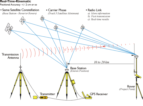
GPS work is sometimes divided into three categories; positioning, navigation, and timing (PNT). Most often, GPS surveying is concerned with the first of these, positioning. In general, there are two techniques used in surveying. They are kinematic and static. In static GPS surveying sessions, the receivers are motionless on the Earth during the observation. Because static work most often provides higher accuracy and more redundancy than kinematic work, it is usually done to establish control. The results of static GPS surveying are processed after the session is completed. In other words, the data is typically post-processed. The majority of GPS surveying control and geodetic work still relies on static applications.
In kinematic GPS surveying, the receivers are either in periodic or continuous motion. Kinematic GPS is done when real-time, or near real-time, results are needed. When the singular objective of kinematic work is positioning, the receivers move periodically using the start and stop methodology originated by Dr. Benjamin Remondi in the 1980s. When the receivers are in continuous motion, the objective may be acquisition of the location, attitude, and velocity of a moving platform (i.e., navigation), or positioning. The distinction between navigation and positioning is lessening.
Kinematic applications imply movement, one or more GPS receivers actually in motion during their observations. A moving GPS receiver on land, sea, or air is characteristic of kinematic GPS. Other characteristics of the application include results in real time and little redundancy. Hydrography, aerial mapping, gravimetric, and more and more land surveying projects are done using kinematic GPS.
Relative positioning is different than autonomous positioning. An independent receiver, an autonomous receiver, must rely on the information in the Navigation Message. In that sort of configuration, it has no way to improve on the corrections. In relative (aka differential) positioning, there are two receivers; one on a known point whose coordinates are well-established, and a second receiver on an unknown point. With this arrangement, the new unknown position can be established relative to the known point. Relative (differential) positioning creates solutions that are positionally superior to autonomous positioning, in large part because it is possible to improve on the corrections available in the Navigation Message.

The term differential GPS, or DGPS, has come into common usage as well. Use of this acronym usually indicates a method of relative positioning where usually coded pseudorange measurements are used rather than carrier phase, though it is sometimes used in context of carrier phase solutions.
The Navigation Solution

Another type of point positioning is known as absolute positioning, single-point positioning, or the Navigation solution. It is characterized by a single receiver measuring its range to a minimum of four satellites simultaneously. An autonomous GPS positioning is not post-processed, and there is really no communication with a station that's on a known point. In other words, autonomous positioning is not differential (relative); the receiver is operating independently. As always, four satellites are required, as indicated here. The receiver is on an unknown position and must solve for its own receiver clock error. It needs to solve for x, y, z, and time. The Navigation solution is, in one sense, the fulfillment of the original idea behind GPS. It relies on a coded pseudorange measurement and can be used for virtually instantaneous positioning. In this method, the positions of the satellites are available from the data in their broadcast ephemerides. The satellite clock offset, and the ionospheric correction are also available from the Navigation messages of all four satellites. As you know, these corrections from that message are not ideal. Even if all the data in the navigation message contained no errors, and they surely do, four unknowns remain: the position of the receiver in three Cartesian coordinates, ux , uy , and uz , and the receiver’s clock error dTu . Three pseudoranges provide enough data to solve for ux , uy , and uz . And the fourth pseudorange provides the information for the solution of the receiver’s clock offset. The ability to measure dT, the receiver’s clock error, is one reason the moderate stability of quartz crystal clock technology is entirely adequate as a receiver oscillator. A unique solution is found here because the number of unknowns is not greater than the number of observations. The receiver tracks a minimum of 4 satellites simultaneously; therefore, these four equations can be solved simultaneously for every epoch of the observation. An epoch in GPS is a very short period of observation time (i.e. 1 second or perhaps less), and is generally just a small part of a longer measurement. However, theoretically, there is enough information in any single epoch to solve these equations. This is the reason the trajectory of a receiver in a moving vehicle can be determined by this method. With 4 satellites available, resolution of a receiver’s position and velocity are both available through the simultaneous solution of these four equations.
Relative Positioning
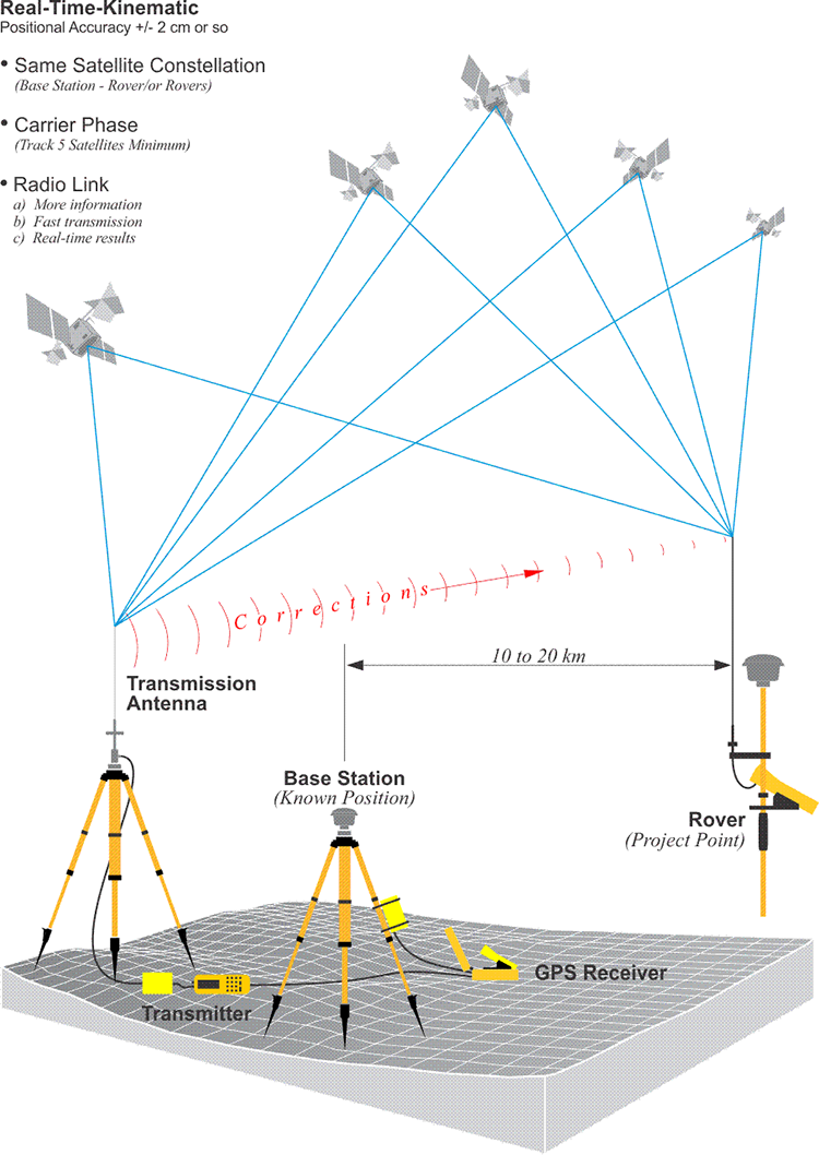
One receiver is employed in single point positioning. A minimum of two receivers are involved in relative or differential positioning. The term differential GPS, or DGPS, sometimes indicates the application of this technique with coded pseudorange measurements, whereas relative GPS usually indicates the application of this technique with carrier phase measurements. However, these definitions are by no means universal, and the use of the terms relative and differential GPS have become virtually interchangeable.
In relative positioning, one of the two receivers involved occupies a known position during the session. It is the base. The objective of the work is the determination of the position of the other, the rover, relative to the base. Both receivers observe the same constellation of satellites at the same time, and because, in typical applications, the vector between the base and the rover, known as a baseline, is so short compared with the 20,000-km altitude of the GPS satellites, there is extensive correlation between observations at the base and the rover. In other words, the two receivers record very similar errors (biases), and since the base’s position is known, corrections can be generated there that can be used to improve the solution at the rover.
If the carrier phase observable is used in relative positioning, baseline measurement accuracies of ± (1 cm + 2 ppm) are achievable. It is possible for GPS measurements of baselines to be as accurate as 1 ppm or even 0.1 ppm. If realized, that would mean that the measurement of a nine-mile baseline would approach its actual length within ±0.05 ft. (1 ppm) or ±0.005 ft. (0.1 ppm).

The autonomous solution can be contrasted with relative positioning or differencing. In this image, you see a GPS receiver working at the same time as a continuously operating reference station that is on a known point. Both are collecting the same constellation of six satellites. And the CORS station (Continuously Operating Reference Station), downloads its observations to an archive. This is a base station archive that, in fact, can be made available on the Internet, as the National Geodetic Survey does. The GPS receiver can download its data at an unknown point to its memory. Post-mission, the two data sets can be brought together and post-processed on a computer. The corrections can be derived from the fact that the Continuously Operating Reference Station knows where it is. This allows the solution at the GPS receiver at the unknown point to be corrected to its actual position relative to the CORS. This is relative positioning. The vector between such a pair of receivers is known as a baseline. It's the simultaneity —in other words, the fact that they're observing the same constellation at the same time— that makes it possible to do accurate GPS in this way.
Networks

Network and multireceiver positioning are obvious extensions of relative positioning. Both the creation of a closed network of points by combining individually observed baselines and the operation of three or more receivers simultaneously have advantages. For example, the baselines have redundant measurements and similar, if not identical, range errors (biases). The processing methods in such an arrangement can nearly eliminate many of the biases introduced by imperfect clocks and the atmosphere. These processing strategies are based on computing the differences between simultaneous GPS carrier phase observations.
Differencing

Please recall that the biases in both the pseudorange and the carrier phase equations discussed at the top obscure the true geometric ranges between the receivers to the satellites, which then contaminate the measurement of the baseline between the receivers. In other words, to reveal the actual vectors between two or more receivers used in relative positioning, those errors must be diminished to the degree that is possible. Fortunately, some of those embedded biases can be virtually eliminated by combining the simultaneous observables from the receivers in processes known as differencing. Even though the noise is increased by a factor of two with each differencing operation, it is typically used in commercial data processing software for both pseudorange and carrier phase measurements. There are three types of differencing, the single difference, double difference, and triple difference. Within the single difference category, there are the between-receivers single difference and the between-satellites single difference. Both require that all the receivers observed the same satellites at the same time. In GPS, the word differencing has come to represent several types of simultaneous baseline solutions of combined measurements. One of the foundations of differencing is the idea of the baseline as it is used in GPS. For example, a single difference, also known as a between-receivers difference, can refer to the difference in the simultaneous carrier phase measurements from one GPS satellite as measured by two different receivers. In the illustration, there are two receivers —q and r— observing the same satellite.
Between-Receivers Single Difference
A between-receivers single difference reduces the effect of biases, even though it doesn’t eliminate them. Since the two receivers are both observing the same satellite at the same time, the difference between the satellite clock bias, dt, at the first receiver and dt at the second receiver, Δdt, is obviously zero. Also, since the baseline is typically short compared with the 20,000-km altitude of the GPS satellites, the atmospheric biases and the orbital errors, i.e., ephemeris errors, recorded by the two receivers at each end are similar. This correlation obviously decreases as the length of the baseline increases. Generally speaking, this correlation allows centimeter level carrier phase positioning with baselines up to 10 km or so, and meter level positioning with baselines of a few hundreds of kilometers using pseudorange observations.
The between-receivers single difference provides better position estimates for the receivers by subtracting, differencing, each receiver’s observation equation from the other. For example, if one of the receivers is a base standing at a control station whose position is known, it follows that the size of the positional error of the receiver there is knowable. Therefore, the positional error at the other end of the baseline can be estimated by finding the difference between the biases at the base and the biases at the rover. Corrections can then be generated which can reduce the three-dimensional positional error at the unknown point by reducing the level of the biases there. It is primarily this correlation and the subsequent ability to reduce the level of error that distinguishes differenced relative positioning from single point positioning.

The between-satellites single difference involves a single receiver observing two GPS satellites simultaneously and the code and/or phase measurement of one satellite are differenced, subtracted, from the other. The data available from the between-satellites difference allows the elimination of the receiver clock error because there is only one involved. And the atmospheric effects on the two satellite signals are again nearly identical as they come into the lone receiver, so the effects of the ionospheric and tropospheric delays are reduced. However, unlike the between-receivers single difference, the between-satellites single difference does not provide a better position estimate for the receiver involved. In fact, the resulting position of the receiver is not better than would be derived from single point positioning.

When the two types of single differences are combined, the result is known as a double difference. A double difference can be said to be a between-satellite single difference of a between-receiver single difference. The improved positions from the between-receiver single difference step are not further enhanced by the combination with the between-satellite single difference. Still, including the between-satellite single difference is useful because the combination virtually eliminates clock errors, both the satellite and receiver clock errors. The removal of the receiver clock bias in the double difference makes it possible to segregate the errors attributable to the receiver clock biases from those from other sources. This segregation improves the efficiency of the estimation of the integer cycle ambiguity in a carrier phase observation, N. In other words, the reduction of all the non-integer biases makes the computation of the final accurate positions more efficient.
The double difference, for all practical purposes, has eliminated the receiver clock errors and the satellite clock errors. This is used in most GPS post-processing and software. The integer ambiguity, N, still remains with the carrier phase observation.

A triple difference is the difference of two double differences over two different epochs. The triple difference has other names. It is also known as the receiver satellite-time triple difference and the between-epochs difference. Triple differencing serves as a good pre-processing step, because it can be used to detect and repair cycle slips.
Cycle Slip

Here's a graphic to give the idea of a cycle slip. As you see here, the cycle slip is indicated in a double difference, here, as a jump from one place to another. And in a triple difference, it's a spike.
A cycle slip is a discontinuity in a receiver’s phase lock on a satellite’s signal. A power loss, a very low signal-to-noise ratio, a failure of the receiver software, a malfunctioning satellite oscillator can cause a cycle slip. It can also be caused by severe ionospheric conditions. Most common, however, are obstructions such as buildings, trees, etc., that are so solid they prevent the satellite signal from being tracked by the receiver. Under such circumstances, when the satellite reappears, the tracking resumes.
Coded pseudorange measurements are not as affected by cycle slips as are carrier phase measurements. On the other hand, carrier phase positioning accuracy suffers if cycle slips are not detected and repaired. A cycle slip causes the critical component for successful carrier phase positioning, a resolved integer cycle ambiguity, N, to become instantly unknown again. In other words, lock is lost. When that happens, correct positioning requires that N be reestablished.
There are several methods of handling cycle slips. They are often controlled in post-processing rather than real-time.
Repairing Cycle Slips
In post-processing, the location and their size of cycle slips must be determined; then the data set can be repaired with the application of a fixed quantity to all the subsequent phase observations. One approach is to hold the initial positions of the stations occupied by the receivers as fixed, and edit the data manually. This has proven to work, but would does try patience. Another approach is to model the data on a satellite-dependent basis with continuous polynomials to find the breaks and then manually edit the data set a few cycles at a time. In fact, several methods are available to find the lost integer phase value, but they all involve testing quantities.
One of the most convenient of these methods is based on the triple difference. It can provide an automated cycle slip detection system that is not confused by clock drift and, once least-squares convergence has been achieved, it can provide initial station positions even using the unrepaired phase combinations. They may still contain cycle slips, but the data can nevertheless be used to process approximate baseline vectors. Then the residuals of these solutions are tested, sometimes through several iterations. Proceeding from its own station solutions, the triple difference can predict how many cycles will occur over a particular time interval. Therefore, by evaluating triple difference residuals over that particular interval, it is not only possible to determine which satellites have integer jumps, but also the number of cycles that have actually been lost. In a sound triple difference solution without cycle slips, the residuals are usually limited to fractions of a cycle. Only those containing cycle slips have residuals close to one cycle or larger. Once cycle slips are discovered, their correction can be systematic.
For example, suppose the residuals of one component double difference of a triple-difference solution revealed that the residual of satellite PRN 16 minus the residual of satellite PRN 17 was 8.96 cycles. Further, suppose that the residuals from the second component double difference showed that the residual of satellite PRN 17 minus the residual of satellite PRN 20 was 14.04 cycles. Then, one might remove 9 cycles from PRN 16 and 14 cycles from PRN 20 for all the subsequent epochs of the observation. However, the process might result in a common integer error for PRNS 16, 17, and 20. Still, small jumps of a couple of cycles can be detected and fixed in the double-difference solutions. In other words, before attempting double difference solutions, the observations should be corrected for cycle slips identified from the triple difference solution. And even though small jumps undiscovered in the triple difference solution might remain in the data sets, the double difference residuals will reveal them at the epoch where they occurred. However, some conditions may prevent the resolution of cycle slips down to the one-cycle level. Inaccurate satellite ephemerides, noisy data, errors in the receiver’s initial positions, or severe ionospheric effects all can limit the effectiveness of cycle-slip fixing. In difficult cases, a detailed inspection of the residuals might be the best way to locate the problem.
Components of the Carrier Phase Observable

Components of the carrier phase observable
From the moment a receiver locks onto a satellite to the end of the observation, the carrier phase observable can be divided into three parts. Two of them do not change during the session, and one of them does change. The fractional initial phase is established at the first instant of the lock-on. When the receiver starts tracking the satellite, it is highly unlikely to acquire the satellite’s signal precisely at the beginning of a wavelength's phase cycle. It will grab on at some fractional part of a phase, and this fractional phase will remain unchanged for the duration of the observation. It is called the fractional initial phase or the phase measurement and is symbolized in the equation above by . The integer cycle ambiguity N represents the number of full phase cycles between the receiver and the satellite at the first instant of the receiver’s lock-on. It can also be labeled the carrier phase ambiguity or the cycle count at lock-on. It does not change from the moment of the lock to the end of the observation, unless that lock is lost. But when there is a cycle slip, lock is lost, and by the time the receiver reacquires the signal, the normally constant integer ambiguity has changed. In that case, the receiver loses its place in its count of the integer number of cycles is lost. The value ß is the count of the number of full phase cycles coming in throughout the observation. Of course, the count grows from the moment of lock on until the end of the observation. In other words, ß is the receiver’s record of the consecutive change in full phase cycles, 1, 2, 3, 4 . . ., between the receiver and the satellite as the satellite flies over. If the observation proceeds without cycle slips, the observed cycle count is the only one of three numbers that changes.
You may remember from the first lesson that when a GPS receiver locks onto a signal from a satellite, it can acquire the fractional initial phase, α. It can interpret that fractional initial phase by comparing what's coming in from the satellite with the replica frequency that it has on-board in its circuits. That comparison can take place pretty quickly, and it doesn't need to change through the observation of that satellite by that receiver. You may also remember that in an EDM measurement, since it is two-way, the EDM can send out frequencies of different lengths to resolve the cycle ambiguity. GPS doesn't have that advantage. It's a one-way system with set carrier wavelengths, so N is somewhat elusive. As the satellite moves along its orbit, the GPS receiver does observed cycle count. In other words, it can count the number of full wavelengths, ß, since its lock-on, and how much they have changed as the satellite moves from one place to another in its orbit. Armed with an initial pseudorange solution, the receiver can estimate the integer ambiguity (carrier phase ambiguity), N. The initial pseudorange observation gives the receiver an idea how many full cycles there are in that N value. From that starting place, it can use a double difference to nail down that carrier phased ambiguity. Perhaps you have heard the fixed solution terminology in post-processing software in GPS. It is often mentioned as opposed to a float solution. A fixed solution means that the integers are fixed. The N has been solved. A fixed solution is superior to a float solution.
Just to reiterate this— the first fractional initial phase occurs at the first instant of lock-on. The receiver starts tracking the incoming phase from the satellite. It can't yet know how to achieve the perfect synchronization. Lacking this knowledge, the receiver grabs on to the satellite's incoming signal at some fractional part. This fractional part does not change for the duration of the observation. The integer number of cycles (the carrier phase ambiguity) is the integer number of cycles of phase that are present at the moment of lock-on. The observed cycle count is the receiver's consecutive counting of the change in full phase cycles between the receiver and the satellite as the satellite flies over. Of these three terms, ß is the only number that changes. That is, if the observation proceeds correctly. In other words, without any cycle slips. In the carrier phase observation, there are two values that do not change: the fractional initial phase and the integer cycle ambiguity, N. Only the cycle count changes, unless, of course, there's a cycle slip. When lock is lost, a cycle slip occurs. It can be a power loss, an obstruction, low signal to noise ratio (SNR), anything that breaks the signal from the satellite to the receiver. When there is a cycle slip, the receiver loses its place and its count of the number of cycles, the integer lock is also lost, and re-initialization is necessary.
Fixing Cycle Slips
In carrier phase post-processing, the first solution is typically a simple pseudorange single point position at each end of the baseline. These code solutions provide the approximate position of each of the two receiver’s antennas. Each position establishes a search area, a three-dimensional volume of uncertainty, the size of which is defined by the accuracy of the code solution. The correct position of the receiver is contained within it somewhere. The computational time required to find it depends on the size of the search area. Next, cycle slips are addressed because the subsequent instantaneous phase jumps will defeat the upcoming double differencing. Triple differencing is not as affected by cycle slips and is insensitive to integer ambiguities, so it typically precedes double differencing and is used to clean the data by detecting and repairing cycle slips. In fact, pre-processing using the triple difference to weed out and fix cycle slips is one of its primary appeals. As to detection, when a large residual appears in one of the triple difference’s component double differences, it is likely caused by a cycle slip, so the satellite pairs can be sorted until the offending signal is singled-out and repaired. Triple differencing can also provide first positions for the receivers. While the receiver coordinates that result are usually more accurate than pseudorange solutions, their geometric strength is weak and not sufficiently accurate for determining short baselines. Nevertheless, they provide a starting point for the more accurate double-difference solutions that follow.
Discussion
Discussion Instructions
To continue the discussion begun by this lesson, I would like to pose this question:
Consider the effect of biases in the GPS error budget on the measurement of the length of a baseline between two GPS receivers. What differences can you think of between their effect on the measurement of a long baseline as opposed to a short one?
To participate in the discussion, please go to the Lesson 2 Discussion Forum in Canvas. (That forum can be accessed at any time by going to the GEOG 862 course in Canvas and then looking inside the Lesson 2 module.)
Summary
Differencing is an ingenious approach to minimizing the effect of biases in both pseudorange and carrier phase measurements. It is a technique that largely overcomes the impossibility of perfect time synchronization. Double differencing is the most widely used formulation. Double differencing still contains the initial integer ambiguities, of course. And the estimates of the ambiguities generated by the initial processing are usually not integers; in other words, some orbital errors and atmospheric errors remain. But with the knowledge that the ambiguities ought to be integers, during subsequent processing, it is possible to force estimates for the ambiguities that are, in fact, integers. When the integers are so fixed, the results are known as a fixed solution, rather than a float solution. It is the double differenced carrier phase based fixed solution that makes the very high accuracy possible with GPS.
However, it is important to remember that multipath, cycle slips, incorrect instrument heights, and a score of other errors whose effects can be minimized or eliminated by good practice are simply not within the purview of differencing at all. The unavoidable biases that can be managed by differencing— including clock, atmospheric, and orbital errors—can have their effects drastically reduced by the proper selection of baselines, the optimal length of the observation sessions, and several other considerations included in the design of a GPS survey. But such decisions require an understanding of the sources of these biases and the conditions that govern their magnitudes. The adage of, “garbage in, garbage out,” is as true of GPS as any other surveying procedure. The management of errors cannot be relegated to mathematics alone.
Before you go on to Lesson 3, double-check the Lesson 2 Checklist to make sure you have completed all of the activities listed there.
Lesson 3: The Framework
The links below provide an outline of the material for this lesson. Be sure to carefully read through the entire lesson before returning to Canvas to submit your assignments.
Lesson 3 Overview
Overview
The Department of Defense found nearly 120 different types of positioning systems in place in the 1970s. They were all limited in their application and local in their scope. Consolidation was called for. NAVSTAR GPS (NAVigation System with Timing And Ranging, Global Positioning System) was proposed. The new system was built on the strengths and avoided the weaknesses of its forerunners.
In this lesson, we will take a look at the earlier systems and their technological contributions toward the development of GPS. This is not history for its own sake. It is an effort to explain the reasons behind the functioning of the GPS system today, built as it is on lessons learned from experience.
Objectives
At the successful completion of this lesson, students should be able to:
- discuss technological forerunners of GPS;
- recognize terrestrial radio positioning, optical systems, and extraterrestrial radio positioning;
- explain the role of TRANSIT in GPS development;
- explain NAVSTAR;
- describe GPS Segment Organization; and
- differentiate between the roles of the Space Segment, the Control Segment, and the User Segment.
Questions?
If you have any questions now or at any point during this week, please feel free to post them to the Lesson 3 Discussion Forum. (To access the forum, return to Canvas and navigate to the Lesson 3 Discussion Forum in the Lesson 3 module.) While you are there, feel free to post your own responses if you, too, are able to help out a classmate.
Checklist
Lesson 3 is one week in length. (See the Calendar in Canvas for specific due dates.) To finish this lesson, you must complete the activities listed below. You may find it useful to print this page out first so that you can follow along with the directions.
| Step | Activity | Access/Directions |
|---|---|---|
| 1 | Read the lesson Overview and Checklist. | You are in the Lesson 3 online content now. The Overview page is previous to this page, and you are on the Checklist page right now. |
| 2 | Read Chapter 3 in GPS for Land Surveyors. | Text |
| 3 | Read the lecture material for this lesson. | You are currently on the Checklist page. Click on the links at the bottom of the page to continue to the next page, to return to the previous page, or to go to the top of the lesson. You can also navigate the lecture material via the links in the Lessons menu. |
| 4 | Participate in the Discussion. | To participate in the discussion, please go to the Lesson 3 Discussion Forum in Canvas. (That forum can be accessed at any time by going to the GEOG 862 course in Canvas and then looking inside the Lesson 3 module.) |
| 5 | Take the Lesson 3 Quiz. (This quiz will cover Lessons 1, 2, and 3.) | The Lesson 3 Quiz is located in the Lesson 3 module in Canvas. |
| 6 | Read lesson Summary. | You are in the Lesson 3 online content now. Click on the "Next Page" link to access the Summary. |
Technological Forerunners

In the early 1970s, the Department of Defense, DOD, commissioned a study to define its future positioning needs. That study found nearly 120 different types of positioning systems in place, all limited by their special and localized requirements. They were of various kinds—some were terrestrial, some relied on electromagnetic signals, some were optical. There were various kinds of positioning systems in place. A plan was made to combine the systems—to integrate them. In general, the idea always was to take from the previous systems the aspects that worked the best and to leave behind those that left something to be desired. The study called for consolidation, and NAVSTAR GPS (NAVigation System with Timing And Ranging, Global Positioning System) was proposed. Specifications for the new system were developed to build on the strengths and avoid the weaknesses of its forerunners. What follows is a brief look at the earlier systems and their technological contributions toward the development of GPS.
Terrestrial Radio Positioning

As mentioned, many of the systems were terrestrial. And, of course, RADAR (RAdio Detecting And Ranging) in its earliest configuration was one of those. During World War II, it was a powerful tool. Long before the satellite era, the developers of RADAR were working out many of the concepts and terms still used in electronic positioning today. For example, the classification of the radio portion of the electromagnetic spectrum by letters, such as the L-band used in naming the GPS carriers, was introduced during World War II to maintain military secrecy about the new technology.
Electromagnetic Spectrum

Above is a chart of a portion of the electromagnetic spectrum. Visible light is a very small range in the middle. Microwaves—which is the area where the RADAR bands live—is considerably outside the visible range.
The 23cm wavelength that was originally used for search radar was given the L designation because it was long compared to the shorter 10cm wavelengths introduced later. The L band wavelengths are 15 to 30 centimeters. So, when we say L band, we're referring to this identification system. The GPS carriers with wavelengths in the neighborhood of 20 centimeters fit well within that context. The shorter wavelength was called S-band, the S for short. The S band—s for short—8 to 15 centimeters. But the Germans used even shorter wavelengths of 1.5cm. They were called K-band, for kurtz, meaning short in German. Wavelengths that were neither long nor short were given the letter C, for compromise, and P-band, for previous, was used to refer to the very first meter-length wavelengths used in RADAR. There is also an X-band radar used in fire-control radars and other applications. In any case, the concept of measuring distance with electromagnetic signals (ranging in GPS) had one of its earliest practical applications in RADAR. Since then, there have been several incarnations of the idea.
Shoran station

Shoran (SHOrt RAnge Navigation), a method of electronic ranging using pulsed 300 MHz VHF (very-high-frequency) signals, was designed for bomber navigation, but was later adapted to more benign uses. The system depended on a signal, sent by a mobile transmitter-receiver-indicator unit being returned to it by a fixed transponder. The elapsed time of the round trip was then converted into distances. It was not long before the method was adapted for use in surveying. Using Shoran from 1949 to 1957, Canadian geodesists were able to achieve precisions as high as 1:56,000 on lines of several hundred kilometers. The ability to measure distances of this magnitude was extraordinary in those times. Shoran was used in hydrographic surveys in 1945 by the United States Coast and Geodetic Survey. In 1951, Shoran was used to locate islands off Alaska in the Bering Sea that were beyond positioning by visual means. Also in the early 1950s, the U.S. Air Force created a Shoran measured trilateration net between Florida and Puerto Rico that was continued on to Trinidad and South America. Trilateration is a familiar term now, as it has come up again in GPS—positioning based upon distances. However, it's worthwhile to note that Shoran and the related technologies, Loran and Hiran, are terrestrial based.
Shoran’s success led to the development of Hiran (high-precision Shoran). Hiran’s pulsed signal was more focused, its amplitude more precise, and its phase measurements more accurate. Hiran was also applied to geodesy. It was used to make the first connection between Africa, Crete, and Rhodes in 1943. But its most spectacular application were the arcs of triangulation joining the North American Datum (1927) with the European Datum (1950) in the early 1950s. By knitting together continental datums, Hiran surveying might be considered to be the first practical step toward positioning on a truly global scale.
Hiran surveying

Hiran surveying was really the first intercontinental system. As you can see in this graphic, it was used to connect datums across the oceans. This had never been done before. It was especially remarkable given that this was a terrestrial system. Up until we started thinking in global terms, there was really no reason to consider that a worldwide foundation of measurement was needed. Today, it is usual to think of the whole planet, and we expect measurements to be consistent around the Earth. However, before intercontinental connections were made, that idea wasn't necessary or taken seriously. So, one of the forerunners of GPS is simply the mindset of thinking in terms of a global datum (reference frame).
Satellites

These and other radio navigation systems proved that ranges derived from accurate timing of electromagnetic radiation were viable. But useful as they were in geodesy and air-navigation, they only whet the appetite for a higher platform. In 1957, the development of Sputnik, the first earth-orbiting satellite, made that possible.
Some of the benefits of earth-orbiting satellites were immediately apparent. It was clear that the potential coverage was virtually unlimited. But other advantages were less obvious.
Sputnik didn't really do anything but send a pulse that was identifiable by any shortwave enthusiast around the world. Nevertheless, its success led to a great awakening to the possibilities of orbiting artificial satellites. It was obvious that a platform that high, broadcasting electromagnetic signals, would be able to cover the entire planet much more effectively than any terrestrial system, even Hiran, could manage. In fact, there were other aspects of the Sputnik signal we're still using today in GPS.
Satellite advantages

It was clear that the potential coverage was virtually unlimited. The coverage of a terrestrial radio navigation system is limited by the propagation characteristics of electromagnetic radiation near the ground. To achieve long ranges, the basically spherical shape of the earth favors low frequencies that stay close to the surface. You've undoubtedly heard of the bouncing of radio waves off the ionosphere, for example. One such terrestrial radio navigation system, LORAN-C ( LOng-RANge navigation-C), was used to determine speeds and positions of receivers up to 3000 km from fixed transmitters. Unfortunately, its frequency had to be in the LF (Low-Frequency range) from 90 to 110 kHz. Many nations besides the United States used LORAN including Japan, Canada, and several European countries. Russia has a similar system called Chayka. In any case, LORAN was phased out in the United States and Canada in 2010, though eLORAN (enhanced LORAN) continues to be considered. These low frequency systems were used to do positioning. But were not intended to be at the level of accuracy of GPS.

Omega, another low frequency hyperbolic radio navigation system, was operated from 1968 to September 30, 1997 by the United States Coast Guard. Omega was used by other countries as well. It was capable of ranges of 9000 km. Its 10- to 14-kHz frequency was so low as to be audible (the range of human hearing is about 20 Hz to 20 kHz). Such low frequencies can be profoundly affected by unpredictable ionospheric disturbances and ground conductivity, making modeling the reduced propagation velocity of a radio signal over land difficult. However, higher frequencies require line of sight.
Line of sight is no problem for earth-orbiting satellites, of course. Signals from space overcome many of the low frequency limitations, allow the use of a broader range of frequencies, and are simply more reliable. Using satellites, one could achieve virtually limitless coverage. Earth-orbiting satellites allow the use of high frequencies. They can cover the entire planet. But development of the technology for launching transmitters with sophisticated frequency standards into orbit was not accomplished immediately. Launching such transmitters, frequency standards, oscillators, etc., into orbit was a pretty tall order in 1957 when Sputnik went up. Therefore, some of the earliest extraterrestrial positioning was done with optical systems.
Optical Systems
Some of the earliest extraterrestrial positioning was done with optical systems. Optical tracking of satellites is a logical extension of astronomy. The astronomic determination of a position on the earth’s surface from star observations, certainly the oldest method, is actually very similar to extrapolating the position of a satellite from a photograph of it crossing the night sky. In fact, the astronomical coordinates, right ascension α and declination δ, of such a satellite image are calculated from the background of fixed stars.
Here's a picture of a track of the International Space Station against the so-called fixed stars. Of course, it is possible to determine the position of a satellite in this way because the stars have known coordinates in the right ascension and declination system. And so, if one knows the time and knows the stars in the background, it is quite possible to learn the ephemeris—or the position—of the satellite based upon that control. This is an extension of astronomy that has been used—and to some extent continues to be used—in terms of positioning the satellites. For example, it's worth noting that some of the major remote sensing satellites have star trackers on board that help determine their orientation and position.

Photographic images that combine reflective satellites and fixed stars are taken with ballistic cameras whose chopping shutters open and close very fast. The technique causes both the satellites, illuminated by sunlight or earth-based beacons, and the fixed stars to appear on the plate as a series of dots. Comparative analysis of photographs provides data to calculate the orbit of the satellite. Photographs of the same satellite made by cameras thousands of kilometers apart can thus be used to determine the camera’s positions by triangulation. The accuracy of such networks has been estimated as high as ±5 meters.
Of course, by implication, if one knows the position of a satellite relative to a sensor on the Earth's surface, then, obviously, it is possible to extrapolate the position of the sensor on the Earth's surface. The result is a positioning system that uses extraterrestrial objects to determine positions on the Earth's surface. The idea of using satellites to get positions on the Earth has a history of many decades.

Other optical systems are much more accurate. One called SLR (Satellite Laser Ranging) is similar to measuring the distance to a satellite using a sophisticated EDM. A laser aimed from the earth to satellites equipped with retro reflectors yields the range. It is instructive that all new GNSS satellites, except GPS, are equipped with lasers onboard corner cube reflectors (aka Laser Retroreflector Arrays, LRAs) for exactly this purpose. The GPS space vehicles numbered SVN 35 (PRN 05) and SVN 36 (PRN 06) were equipped with LRAs, thereby allowing ground stations to separate the effect of errors attributable to satellite clocks from errors in the satellite’s ephemerides. Neither of them is still in service, but the plan is to have LRAs on all upcoming GPS III satellites.
The same technique, called LLR (Lunar Laser Ranging), is used to measure distances to the moon using corner cube reflector arrays left there during manned missions. There are four available arrays - three of them set during Apollo missions and one during the Soviet Lunokhod 2 mission. These techniques can achieve positions of centimeter precision when information is gathered from several stations. However, one drawback is that the observations must be spread over long periods, up to a month, and they, of course, depend on two-way measurement.
We discussed EDMs earlier, and you know that it is possible to use EDMs as an optical system to determine distances. Satellite Laser Ranging, SLR, can measure distances using an electronic distance measuring device, an EDM, and a laser that points from the Earth to the satellite. The reflectors on the satellite can return that signal to the terrestrial sensor. This a method of measurement by phase comparison with a reference wave at the EDM. It works well for satellites orbiting. This system is also used for Lunar Laser Ranging (LLR). There are banks of reflecting retro prisms on the lunar surface that were left by the manned missions, both Russian and American. We can now determine the position of the moon relative to the Earth using electronic distance measuring to centimeter precision. This is useful for many positioning needs.
Optical drawbacks

While some optical methods, like SLR, can achieve extraordinary accuracies, they can at the same time be subject to chronic difficulties. Some methods require skies to be clear at widely spaced sites simultaneously. Even then, the troposphere and the ionosphere can be very uncooperative. And local atmospheric turbulence can cause the images of the satellites to scintillate. The necessity of broadcasting a signal revealing your position, the need to have expensive—and sometimes bulky—equipment and the difficulty of modeling optical refraction are some of the drawbacks to the optical method. Still, it remains a significant part of the satellite management programs of NASA and other agencies.
Extraterrestrial Systems

The earliest American extraterrestrial systems were designed to assist in satellite tracking and satellite orbit determination, not geodesy. Some of the methods used did not find their way into the GPS technology at all. Some early systems relied on the reflection of signals, transmissions from ground stations, that would either bounce off the satellite or stimulate onboard transponders. But systems that required the user to broadcast a signal from the earth to the satellite were not favorably considered in designing the then-new GPS system. Any requirement that the user reveal his position was not attractive to the military planners responsible for developing GPS. They favored a passive system that allowed the user to simply receive the satellite’s signal. So, with their two-way measurements and utilization of several frequencies to resolve the cycle ambiguity, many early extraterrestrial tracking systems were harbingers of the modern EDM technology more than GPS.
But, elsewhere, there were ranging techniques useful to GPS. NASA's first satellite tracking system, Prime Minitrack, relied on phase difference measurements of a single-frequency carrier broadcast by the satellites themselves and received by two separate ground-based antennas. This technique is called interferometry. Interferometry is the measurement of the difference between the phases of signals that originate at a common source but travel different paths to the receivers. The combination of such signals, collected by two separate receivers, invariably finds them out of step (out of phase) since one has traveled a longer distance than the other. Analysis of the signal’s phase difference can yield very accurate ranges, and interferometry has become an indispensable measurement technique in several scientific fields. Interferometry was used in the first commercial GPS receiver, called a Macrometer.
VLBI

For example, Very Long Baseline Interferometry (VLBI) did not originate in the field of satellite tracking or aircraft navigation, but in radio astronomy. The technique was so successful it is still in use today. Radio telescopes, sometimes on different continents, tape-record the microwave signals from quasars, star-like points of light billions of light-years from earth. A quasar is a very consistent radio source in the sky, and tracking these quasars from radio telescopes can be used to measure extraordinary distances very accurately using interferometry. The technique is used today in the network of control points around the globe for monitoring tectonic movements which is one of the technologies at the foundation of the International Terrestrial Reference Frame (ITRF), which we will talk about later.
In any case, these recordings are encoded with time tags controlled by hydrogen masers, the most stable of oscillators (clocks). The tapes are then brought together and played back at a central processor. Cross-correlation of the time tags reveals the difference in the instants of wavefront arrivals at the two telescopes. The discovery of the time offset that maximizes the correlation of the signals recorded by the two telescopes yields the distance and direction between them within a few centimeters, over thousands of kilometers.
VLBI’s potential for geodetic measurement was realized as early as 1967. But the concept of high-accuracy baseline determination using phase differencing was really proven in the late 1970s. A direct line of development leads from the VLBI work of that era by a group from the Massachusetts Institute of Technology to today’s most accurate GPS ranging technique, carrier phase measurement. VLBI, along with other extraterrestrial systems like SLR, also provides valuable information on the earth’s gravitational field and rotational axis. It has become possible through extraterrestrial means to combine the datums of different continents, the shape of the Earth and the orientation of the Earth. Without that data, the high accuracy of the modern coordinate systems that are critical to the success of GPS, like the Conventional Terrestrial System (CT), would not be possible. But the foundation for routine satellite-based geodesy actually came even earlier and from a completely different direction. The first prototype satellite of the immediate precursor of the GPS system that was successfully launched reached orbit on June 29, 1961. Its range measurements were based on the Doppler Effect, not phase differencing, and the system came to be known as TRANSIT, or more formally the Navy Navigational Satellite System.
Satellite Positioning

Satellite technology and the Doppler Effect were combined in the first comprehensive earth-orbiting satellite system dedicated to positioning. By tracking Sputnik in 1957, experimenters at Johns Hopkins University’s Applied Physics Laboratory found that the Doppler shift of its signal provided enough information to determine the exact moment of its closest approach to the earth. This discovery led to the creation of the Navy Navigational Satellite System (NNSS or NAVSAT) and the subsequent launch of 6 satellites specifically designed to be used for navigation of military aircraft and ships. This same system, eventually known as TRANSIT, was classified in 1964, declassified in 1967, and was widely used in civilian hydrographic and geodetic surveying for many years until it was switched off on December 31, 1996.
The Doppler shift is characterized by the observation that when the source of a constant signal is approaching, its constituent wavefronts are compressed closer together. As that signal source moves away, the wavefronts are pulled further apart. This is often illustrated by the change in pitch of a railroad horn. As the train approaches, the pitch seems to rise, and as it moves away, the pitch seems to fall. The same effect is obvious with the changes in frequency of the signal from a satellite as it passes. As the satellite approaches, the observer wavefronts are pushed together, and as it moves away, they're pulled further apart. The rate at which this happens can be analyzed to determine the position of the observer in a passive way.
TRANSIT shortcomings

The TRANSIT system had some nagging drawbacks. For example, its primary observable was based on the comparison of the nominally constant frequency generated in the receiver with the Doppler-shifted signal received from 1 satellite at a time. With a constellation of only 6 satellites, this strategy sometimes left the observer waiting up to 90 minutes between satellites, and at least two passes were usually required for acceptable accuracy. With an orbit of only about 1100 km above the earth, the TRANSIT satellite’s orbits were quite low and, therefore, unusually susceptible to atmospheric drag and gravitational variations, making the calculation of accurate orbital parameters particularly difficult. Through the decades of the 1970s and 1980s, both the best and the worst aspects of the forerunner system informed GPS development.
In the end many strategies used in TRANSIT were incorporated into GPS. For example, in the TRANSIT system, the satellites broadcast their own ephemerides to the receivers and the receivers had their own frequency standards. TRANSIT had three segments: the control segment, including the tracking and upload facilities; the space segment, meaning the satellites themselves; and the user segment, everyone with receivers. The TRANSIT system satellites broadcast two frequencies of 400 MHz and 150 MHz to allow compensation for the ionospheric dispersion. TRANSIT’s primary observable was based on the Doppler Effect. All were used in GPS.
Perhaps one of the most significant advantages of the TRANSIT system over previous extraterrestrial systems was TRANSIT’s capability of linking national and international datums with relative ease. Its facility at strengthening geodetic coordinates laid the groundwork for modern geocentric datums. In 1963, at about the same time the Navy was using TRANSIT, the Air Force funded the development of a three-dimensional radio navigation system for aircraft. It was called System 621B. The fact that it provided a determination of the third dimension, altitude, was an improvement of some previous navigation systems. It relied on the user measuring ranges to satellites based on the time of arrival of the transmitted radio signals. With the instantaneous positions of the satellites known, the user’s position could be derived. The 621B program also utilized carefully design binary codes known as PRN codes or pseudorandom noise. Even though the PRN codes appeared to be noise at first, they were actually capable of repetition and replication. This approach also allowed all of the satellites to broadcast on the same frequency. Sounds rather familiar now, doesn’t it? Unfortunately, System 621B required signals from the ground to operate.
Another project, this one from the Navy had a name that conflated time and navigation, Timation. It began in 1964. The Timation 1 satellite was launched in 1967; it was followed by Timation 2 in 1969. Both of these satellites were equipped with high performance quartz crystal oscillators also known as XO. The daily error of these clocks was about 1 microsecond, which translates to about 300 m of ranging error. The technique they used to transmit ranging signals was called side-tone ranging. There was a great improvement in the clocks of Timation 3 which was launched in 1974. It was the first satellite outfitted with two rubidium clocks. Being able to have space-worthy Atomic Frequency Standards, AFS, on orbit was a big step toward accurate satellite positioning, navigation and timing (PNT). With this development, the Timation program demonstrated that a passive system using atomic clocks could facilitate worldwide navigation. The terms clock, oscillator, and frequency standard will be used interchangeably here.
It was the combination of atomic clock technology, the ephemeris system from TRANSIT, and the PRN signal design from the 621B program in 1973 that eventually became GPS. There was a Department of Defense directive to the United States Air Force in April 1973 that stipulated the consolidation of TIMATION and 621B into the navigation system called GPS. In fact, Timation 3 became part of the NAVSTAR–GPS program and was renamed Navigation Technology Satellite 1 (NTS-1). The next satellite in line, Timation 4 was known as NTS-2. Its onboard cesium clock had a frequency stability of 2 parts per 1013. It was launched in 1977. Unfortunately, it only operated for 8 months.

NAVSTAR GPS

GPS improved on some of the shortcomings of the previous systems. For example, the GPS satellites were placed in nearly circular orbits over 20,000 km above the earth where the consequences of gravity and atmospheric drag are much less severe than the lower orbits assigned to TRANSIT, Timation, and some of the other earlier systems used. GPS satellites broadcast higher frequency signals, which reduce the ionospheric delay. The rubidium and cesium clocks pioneered in the Timation program and built into GPS satellites were a marked improvement over the quartz oscillators that were used in TRANSIT and other early satellite navigation systems. System 621B could achieve positional accuracies of approximately 16 meters. TRANSIT’s shortcomings restricted the practical accuracy of the system, too. It could achieve submeter work, but only after long occupations on a station (at least a day) augmented by the use of precise ephemerides for the satellites in post-processing. GPS provides much more accurate positions in a much shorter time than any of its predecessors, but these improvements were only accomplished by standing on the shoulders of the technologies that have gone before.
Requirements
The genesis of GPS was military. It grew out of the congressional mandate issued to the Departments of Defense and Transportation to consolidate the myriad of navigation systems. Its application to civilian surveying was not part of the original design. In 1973, the DOD directed the Joint Program Office (JPO) in Los Angeles to establish the GPS system. Specifically, JPO was asked to create a system with high accuracy and continuous availability in real time that could provide virtually instantaneous positions to both stationary and moving receivers in three dimensions. The forerunners could not supply all these features. The challenge was to bring them all together in one system.
Secure, Passive, and Global
Worldwide coverage and positioning on a common coordinate grid were required of the new system—a combination that had been difficult, if not impossible, with terrestrial-based systems. It was to be a passive system, which ruled out any transmissions from the users, as had been tried with some previous satellite systems. The user could not be required to reveal their position when they used the system, so obviously broadcasting a signal was out of the question. The signal was also to be secure and resistant to jamming, so codes in the satellite’s broadcasts would need to be complex and the GPS carriers spread-spectrum (wide).
Spread Spectrum Signal
The specification for the GPS system required all-weather performance and correction for ionospheric propagation delay. TRANSIT had shown what could be accomplished with a dual-frequency transmission from the satellites, but it had also proved that a higher frequency was needed. The GPS signal needed to be secure and resistant to both jamming and multipath. A spread spectrum, meaning spreading the frequency over a band wider than the minimum required for the information it carries, helped on all counts. This wider band also provided ample space for pseudorandom noise encoding, a fairly new development at the time. The PRN codes like those used in System 621B allowed the GPS receiver to acquire signals from several satellites simultaneously and still distinguish them from one another.
Expense and Frequency Allocation
The U.S. Department of Defense (DOD) also wanted the new system to be free from the sort of ambiguity problems that had plagued OMEGA and other radar systems. And DOD did not want the new system to require large, expensive equipment like the optical systems. Finally, frequency allocation was a consideration. The replacement of existing systems would take time, and with so many demands on the available radio spectrum, it was going to be hard to find frequencies for GPS.
Large Capacity Signal
Not only did the specifications for GPS evolve from the experience with earlier positioning systems, so did much of the knowledge needed to satisfy them. Providing 24- hour real-time, high-accuracy navigation for moving vehicles in three dimensions was a tall order. Experience showed part of the answer was a signal that was capable of carrying a large amount of information efficiently and that required a large bandwidth, especially since the system needed to be passive. So, the GPS signal was given a double-sided 10-MHz bandwidth. But that was still not enough, so the idea of simultaneous observation of several satellites was also incorporated into the GPS system to accommodate the requirement. Unlike some of its predecessors, GPS needed to have not one, but at least four satellites above an observer's horizon for adequate positioning. Even more, if possible. And the achievement of full-time worldwide GPS coverage would require this condition be satisfied at all times, anywhere on or near the earth. That decision had far-reaching implications.
The Perfect System?
The absolute ideal navigational system, from the military’s point of view, was described in the Army POS/NAV Master Plan in 1990. It should have worldwide and continuous coverage. The users should be passive. In other words, they should not be required to emit detectable electronic signals to use the system. The ideal system should be capable of being denied to an enemy, and it should be able to support an unlimited number of users. It should be resistant to countermeasures and work in real time. It should be applicable to joint and combined operations. There should be no frequency allocation problems. It should be capable of working on common grids or map datums appropriate for all users. The positional accuracy should not be degraded by changes in altitude or by the time of day or year. Operating personnel should be capable of maintaining the system. It should not be dependent on externally generated signals, and it should not have decreasing accuracy over time or the distance traveled. Finally, it should not be dependent on the identification of precise locations to initiate or update the system. A pretty tall order; GPS lives up to most, though not all, of the specifications.
The objective, of course, was to build the perfect system. And whether or not that's been achieved, there are several of the specifications that have been met rather well with GPS. It's a passive system—there's no need to broadcast any signals. It can be denied—it can be turned off—when the Department of Defense so desires. It's resistant to countermeasures, meaning—spoofing, for example, is a term used to indicate the idea that a bad guy could broadcast a signal that appears to be a GPS signal to try to confuse the receivers.
It works in real time. It should be applicable to joint and combined operations, militarily speaking. And it should be able to work on common grids that are appropriate for all users. This is very true. One of the things that GPS is very good at is taking its native format—in Earth-Centered, Earth-Fixed XYZ coordinates—and transforming them using the microprocessor and the receiver to virtually any well-defined coordinate system. The positional accuracy should not be degraded by changes in altitude nor by the time of the year—time of day or year. Yes, GPS works well at the top of the mountain and down in the valley—well, except for multipath to some degree. And operating personnel should be capable of maintaining the system. It should not be dependent on externally-generated signals. Of course, that's true—the signals come directly from the satellites. It should not have decreasing accuracy over time and distance traveled. GPS has been extraordinarily effective on measuring very long baselines. It's all a pretty tall order, but GPS has lived up to most of it.
GPS

GPS IN CIVILIAN SURVEYING
As mentioned earlier, application to civilian surveying was not part of the original concept of GPS. The civilian use of GPS grew up through partnerships between various public, private, and academic organizations. Nevertheless, while the military was still testing its first receivers, GPS was already in use by civilians. Geodetic surveys were actually underway with commercially available receivers early in the 1980s.
Federal Specifications
The Federal Radionavigation Plan of 1984, a biennial document including official policies regarding radionavigation set the predictable and repeatable accuracy of civil and commercial use of GPS at 100 meters horizontally and 156 meters vertically. This specification meant that the C/A code ranging for Standard Positioning Service could be defined by a horizontal circle with a radius of 100 meters, 95% of the time. GPS was decidedly a Defense Department system. However, it became apparent early on that civilian receivers were doing much better than 100 meters horizontally. Selective Availability, a dithering of the clocks in the GPS satellite, was instituted. When the clocks in the satellite (the oscillators) don't keep their rate to a steady standard, then the positioning derived from them suffers. In this way, Selective Availability intentionally degraded the accuracy available to the civilian C/A code users to the 100 meter horizontally for quite a long time.
Selective Availability was switched off May 2, 2000. It is not a consideration at the moment, but it could be switched back on. I must mention that since surveyors traditionally worked with the carrier phase observable to achieve high accuracy, therefore the dithering of the pseudorange codes which was the characteristic of SA didn't affect surveying positioning. However, for those who used pseudorange (code-phase) receivers primarily, Selective Availability was a problem. Since it has been switched off, of course, the accuracy of those sorts of receivers has improved markedly.
Interferometry

By using interferometry, the technique that had worked so well with Prime Minitrack and VLBI, civilian users were showing that GPS surveying was capable of extraordinary results. In the summer of 1982, a research group at the Massachusetts Institute of Technology (MIT) tested an early GPS receiver and achieved accuracies of 1 and 2 ppm of the station separation. Over a period of several years, extensive testing that confirmed and improved on these results was conducted around the world. In 1984, a GPS network was produced to control the construction of the Stanford Linear Accelerator. This GPS network provided accuracy at the millimeter level. In other words, by using the differentially corrected carrier phase observable instead of code ranging, private firms and researchers were going far beyond the accuracies the U.S. Government expected to be available to civilian users of GPS.
The interferometric solutions made possible by computerized processing developed with earlier extraterrestrial systems were applied to GPS by the first commercial users. The combination made the accuracy of GPS its most impressive characteristic, but it hardly solved every problem. For many years, the system was restricted by the shortage of satellites as the constellation slowly grew. The necessity of having four satellites above the horizon restricted the available observation sessions to a few, sometimes inconvenient, windows of time. Another drawback of GPS for the civilian user was the cost and the limited application of both the hardware and the software. GPS was too expensive and too inconvenient for everyday use, but the accuracy of GPS surveying was already extraordinary in the beginning.
The photo is of an old friend of mine. This was the first commercial GPS receiver, the Macrometer. It was an interferometric receiver. You see here the receiver itself on the floor next to the tripod. It was rather heavy. It took two people to carry it. We transported them in utility vehicles adapted for the purpose. Each Macrometer observed the GPS constellation simultaneously with the other Macrometers. This is the concept we discussed as resulting in relative positioning. Relative positioning requires receivers operating simultaneously. With the Macrometer, unlike current GPS receivers, they had to be brought together and their clocks synced. In other words, the several receivers were cabled together, and their oscillators synced with each other. This had to be done to discover the receiver clock drift that occurred during the mission. It was necessary because the Macrometer was a codeless receiver. It did not have access to the Navigation Message. That meant that the broadcast clock correction and all of the other bias mitigating information in the Navigation Message were unavailable to this particular receiver. All of that had to be done in the post-processing phase.
The antenna of the Macrometer was a meter square of aluminum. You can see the plexiglass dome with a dipole antenna on the underneath of it. And of course, the antenna was cabled to the receiver. You can see the black tape drives on the top of the receiver. We used tapes to record the observations. The system ran on 110 volts. So, we had to carry generators with us. It was quite a beefy system to carry around and quite expensive. Nevertheless, it worked rather well. It was possible to achieve one to two parts per million of the station separation, which was much more accurate than the 100-meter spec we were talking about earlier. This was possible because the system utilized the carrier phase—aka the carrier beat phase—observable. GPS achieved extraordinary accuracy from the very beginning, from the very first commercial GPS receiver. I was proud to be part of it.
Civil Applications of GPS
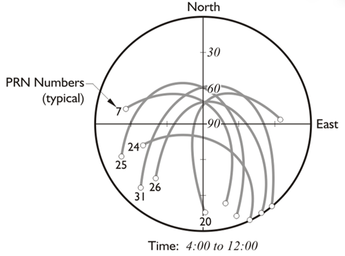
Today, with a mask angle of 10°, there are some periods when 15 or more GNSS satellites are above the horizon. And GPS receivers have grown from only a handful to the huge variety of receivers available today. Some push the envelope to achieve ever-higher accuracy; others offer less sophistication and lower cost. The civilian user’s options are broader with GPS than any previous satellite positioning system—so broad that, as originally planned, GPS will likely replace more of its predecessors in both the military and civilian arenas. In fact, GPS has developed into a system that has more civilian applications and users than military ones. But the extraordinary range of GPS equipment and software requires the user to be familiar with an ever-expanding body of knowledge, including the Global Navigation Satellite System (GNSS). GNSS includes both GPS and satellite navigation systems built by other nations and will present new options for users. However, the three segments of GPS will be presented before elaborating on GNSS.
Continuing on with the civilian point of view, which, of course, is our primary focus; today, with a mask angle of 10 degrees, it's possible to have up to 10 satellites above the horizon. Of course, when we first started, we were very happy when we were able to have four. So, it's obvious that as time goes on, the cost of the receivers keeps going down and their sophistication going up. And GPS, clearly, has been replacing its predecessors in both the military and civilian arenas. In fact, GPS has developed into a system that has more civilian applications and users than military ones. It's really a remarkable story of how rapidly the system has realized its potential.
The Space Segment

Though there has been some evolution in the arrangement, the current GPS constellation under full operational capability consists of 24 satellites. However, there are more satellites than that in orbit and broadcasting at any given time, and the constellation includes several orbital spares.
As the primary satellites aged and their failure was possible, spares were launched. One reason for the arrangement was to maintain the 24 satellite constellation without interruption.
It was also done to ensure that it is possible to keep four satellites, one in each of the four slots in the six orbital planes. Each of these planes is inclined to the equator by 55° in a symmetrical, uniform arrangement. Such a uniform design does cover the globe completely, even though the coverage is not quite as robust at high latitudes as it is at midlatitudes. The uniform design also means that multiple satellite coverage is available even if a few satellites were to fail. The satellites routinely outlast their anticipated design lives, but they are eventually worn out.
Orbital Period
NAVSTAR satellites are more than 20,000 km above the earth in a posigrade orbit. A posigrade orbit is one that moves in the same direction as the earth’s rotation.
The Space Segment includes the satellites themselves. Since each satellite is nearly three times the earth’s radius above the surface, its orbital period is 12 sidereal hours. The sidereal (star time) timescale is different from Mean Solar Time (the normal timescale on which we operate) and different from UTC.
4 minute difference. When an observer actually performs a GPS survey project, one of the most noticeable aspects of a satellite’s motion is that it returns to the same position in the sky about 4 minutes (3 minutes and 56 seconds) earlier each day in our usual Mean Solar Time. This apparent regression is attributable to the difference between 24 solar hours and 24 sidereal hours. This rather esoteric fact has practical applications; for example, if the satellites are in a particularly favorable configuration for measurement, the observer may wish to take advantage of the same arrangement the following day. However, he or she would be well advised to remember the same configuration will occur about 4 minutes earlier on the solar timescale. Both Universal Time (UT) and GPS time are measured in solar, not sidereal units. It is possible that the satellites will be pushed 50 km higher in the future to remove their current 4-minute regression, but, for now, it remains. As mentioned earlier, the GPS constellation was designed to satisfy several critical concerns. Among them were the best possible coverage of the earth with the fewest number of satellites, the reduction of the effects of gravitational and atmospheric drag, sufficient upload, monitoring capability, and the achievement of maximum accuracy.
The Space Segment: Dilution of Precision
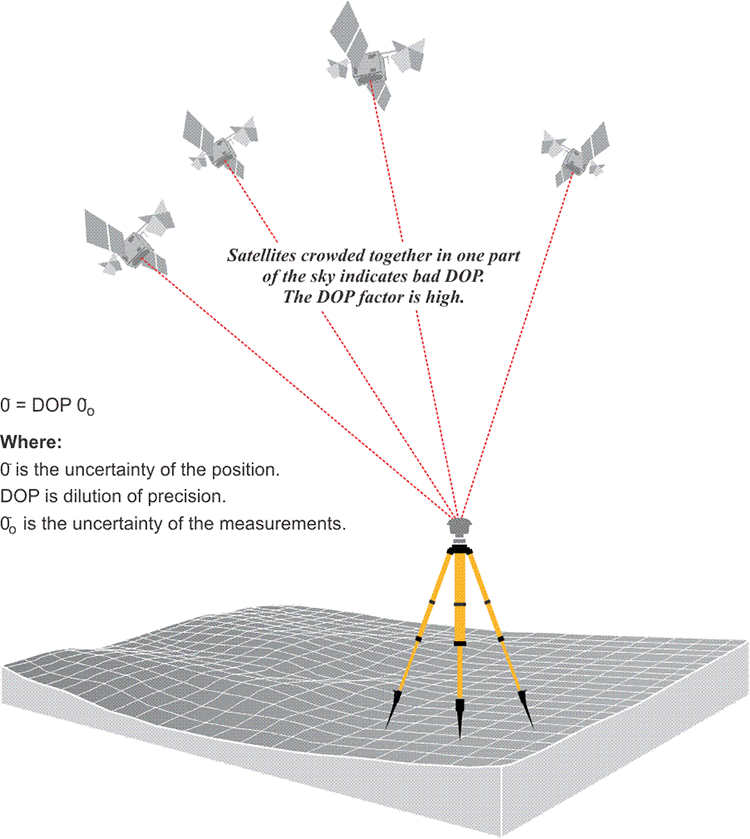
The distribution of the satellites above an observer’s horizon has a direct bearing on the quality of the position derived from them. Like some of its forerunners, the accuracy of a GPS position is subject to a geometric phenomenon called dilution of precision (DOP). This number is somewhat similar to the strength of figure consideration in the design of a triangulation network. DOP concerns the geometric strength of the figure, described by the positions of the satellites with respect to one another and the GPS receivers. A low DOP factor is good, a high DOP factor is bad. In other words, when the satellites are in the optimal configuration for a reliable GPS position, the DOP is low, when they are not, the DOP is high.
Four or more satellites must be above the observer’s mask angle for the simultaneous solution of the clock offset and three dimensions of the receiver’s position. But if all of those satellites are crowded together in one part of the sky, the position would be likely to have an unacceptable uncertainty, and the DOP, or dilution of precision, would be high. In other words, a high DOP is a like a warning that the actual errors in a GPS position are liable to be larger than you might expect. But remember, it is not the errors themselves that are directly increased by the DOP factor; it is the uncertainty of the GPS position that is increased by the DOP factor.

Now, since a GPS position is derived from a three-dimensional solution, there are several DOP factors used to evaluate the uncertainties in the components of a GPS position. For example, there is horizontal dilution of precision (HDOP) and vertical dilution of precision (VDOP) where the uncertainty of a solution for positioning has been isolated into its horizontal and vertical components, respectively. When both horizontal and vertical components are combined, the uncertainty of three-dimensional positions is called position dilution of precision (PDOP). There is also time dilution of precision (TDOP), which indicates the uncertainty of the clock. There is geometric dilution of precision (GDOP), which is the combination of all of the above. And finally, there is relative dilution of precision (RDOP), which includes the number of receivers, the number of satellites they can handle, the length of the observing session, as well as the geometry of the satellites’ configuration.
PDOP is perhaps the most common, which combines both horizontal and vertical. But the idea is very straightforward in the sense that the better the geometry, the better the intersection of the ranges from the satellites, the lower that the dilution of precision value will be and the better the position derived will be. This is a very practical consideration in GPS work.
The user equivalent range error (UERE) is the total error budget affecting a pseudorange. It is the square root of the sum of the squares of the individual biases discussed in Chapter 2. Using a calculation like that mentioned, the PDOP (position dilution of precision) factor can be used to find the positional error that will result from a particular UERE at the one sigma level (68.27%). For example, supposing that the PDOP factor is 1.5 and the UERE is 6 m, the positional accuracy would be 9 m at the 1 sigma level (68.27%). In other words, the standard deviation of the GPS position is the dilution of precision factor multiplied by the square root of the sum of the squares of the individual biases (UERE). Multiplying the 1 sigma value times 2 would provide that 95% level of reliability in the error estimate, which would be 18 m.
The size of the DOP factor is inversely proportional to the volume of the tetrahedron described by the satellites' positions and the position of the receiver. The larger the volume of the body defined by the lines from the receiver to the satellites, the better the satellite geometry and the lower the DOP. An ideal arrangement of four satellites would be one directly above the receiver, the others 120° from one another in azimuth near the horizon. With that distribution, the DOP would be nearly 1, the lowest possible value. In practice, the lowest DOPs are generally around 2. The mask angle plays a part here. If you had four satellites, and three of them were at the horizon and one was directly overhead, this would be a very low dilution of precision value. However, you wouldn't want to track satellites that were right against the horizon. You want them above this mask angle, 10 or 15 degree mask angle, to try to minimize the effect of the ionosphere. The users of most GPS receivers can set a PDOP mask to guarantee that data will not be logged if the PDOP goes above the set value. A typical PDOP mask is 6. As the PDOP increases, the accuracy of the pseudorange positions probably deteriorate, and as it decreases, they probably improve. When a DOP factor exceeds a maximum limit in a particular location, indicating an unacceptable level of uncertainty exists over a period of time, that period is known as an outage. This expression of uncertainty is useful both in interpreting measured baselines and planning a GPS survey.
The Space Segment: Planning
The position of the satellites above an observer’s horizon is a critical consideration in planning a GPS survey. So, most software packages provide various methods of illustrating the satellite configuration for a particular location over a specified period of time. For example, the configuration of the satellites over the entire span of the observation is important; as the satellites move, the DOP changes. Fortunately, the dilution of precision can be worked out in advance. DOP can be predicted. It depends on the orientation of the GPS satellites relative to the GPS receivers. And since most GPS software allow calculation of the satellite constellation from any given position and time, they can also provide the accompanying DOP factors. Another commonly used plot of the satellite’s tracks is constructed on a graphical representation of the half of the celestial sphere. The observer’s zenith is shown in the center and the horizon on the perimeter. The program usually draws arcs by connecting the points of the instantaneous azimuths and elevations of the satellites above a specified mask angle. These arcs then represent the paths of the available satellites over the period of time and the place specified by the user. The plot of the polar coordinates of the available satellites with respect to time and position is just one of several tables and graphs available to help the GPS user visualize the constellation.
It has become common to think that you can simply turn on a GPS receiver and start working under all circumstances. However, the position of the satellites in the sky is critical to good positioning. A polar plot, as illustrated here, shows you the paths of the satellites as if you were looking straight up.

Another useful graph that is available from many software packages. It shows the correlation between the number of satellites above a specified mask angle and the associated PDOP for a particular location during a particular span of time.
There are four spikes of unacceptable PDOP, labeled here for convenience. It might appear at first glance that these spikes are directly attributable to the drop in the number of available satellites. However, please note that while spikes 1 and 4 do indeed occur during periods of 4 satellite data, spikes 2 and 3 are during periods when there are 7 and 5 satellites available, respectively. It is not the number of satellites above the horizon that determine the quality of GPS positions, one must also look at their position relative to the observer, the DOP, among other things. The variety of the tools to help the observer predict satellite visibility underlines the importance of their configuration to successful positioning.
The number of satellites is in the upper part of the chart. The PDOP, position dilution of precision, is in the lower part. Spikes one, two, three and four are areas of very large PDOP. During these moments, the positions that are collected are suspect. Starting at zero hour, the satellites vary between seven and eight, some of them begin to set at two hours. The constellation drops down to four satellites. The four that remain are crowded into one part of the sky. There's a rather extraordinary spike in the PDOP at that point. You wouldn't want to be observing at that time. Shortly thereafter, some satellites rise and the constellation goes back to eight and nine satellites; the PDOP drops below four, and that is a good time to observe.
However, even when there appear to be many satellites above the observer's horizon, there are more spikes in the PDOP. You may wonder why there are spikes if there are so many satellites. It is because the satellites are always moving relative to each other. And even though there are many, they can be crowded together and the PDOP high. At about 12 hours and moving on, the circumstances for observation are good. There are many satellites, the constellation is healthy, above the horizon, and the PDOP is low. However, between 18 and 20 hours, there are just four satellites again, and there is a spike in the PDOP.
So, as you see, it's not really straightforward. The PDOP can be high at any time. It is not correct to say that when the constellation above the horizon is large, the PDOP will be low. It is important to look at it in some detail. It's valuable to note that most processing software packages allow you to easily to make graphs of this type shown here if you have a current ephemeris in your system. And it's lucky that those current ephemerides can be downloaded from the Internet as well as collected from the satellites.
Satellite Blocks


The Control Segment

There are government tracking and uploading facilities distributed around the world. These facilities not only monitor the L-band signals from the GPS satellites and update their Navigation Messages but also track the satellite’s health, their maneuvers, and many other things, even battery recharging. Taken together, these facilities are known as the Control Segment.
The Master Control Station (MCS), once located at Vandenberg Air Force Base in California, now resides at the Consolidated Space Operations Center (CSOC) at Schriever (formerly Falcon) Air Force Base near Colorado Springs, Colorado, and has been manned by the 2nd Space Operations Squadron, 2SOPS, since 1992. There is an alternate MCS at Vandenberg Tracking Station in California. The 2SOPS squadron controls the satellites' orbits. For example, they maneuvered the earlier blocks of satellites from the highly eccentric orbits into which they are originally launched to the desired mission orbit and spacecraft orientation. The Block IIF satellites were placed directly into their intended orbits. They monitor the state of each satellite's onboard battery, solar, and propellant systems. They resolve satellite anomalies, activate spare satellites, and control Selective Availability (SA) and Anti-Spoofing (A/S). They dump the excess momentum from the wheels, the series of gyroscopic devices that stabilize each satellite. With the continuous constellation tracking data available and aided by Kalman filter estimation to manage the noise in the data, they calculate and update the parameters in the Navigation message (ephemeris, almanac, and clock corrections) to keep the information within limits. This process is made possible by a persistent two-way communication with the constellation managed by the Control Segment that includes both monitoring and uploading accomplished through a network of ground antennas and monitoring stations.
The data that feeds the MCS comes from monitoring stations. These stations track the entire GPS constellation. In the past, there were limitations. There were only six tracking stations. It was possible for a satellite to go unmonitored for up to two hours each day. It was clear that the calculation of the ephemerides and the precise orbits of the constellation could be improved with more monitoring stations in a wider geographical distribution. It was also clear that if one of the six stations went down, the effectiveness of the Control Segment could be considerably hampered. These ideas, and others, led to a program of improvements known as the Legacy Accuracy Improvement Initiative, L-AII. During this initiative from August 18 to September 7 of 2005, six National Geospatial Intelligence Agency, NGA, stations were added to the Control Segment. This augmented the information forwarded to the MCS with data from Washington, D.C., England, Argentina, Ecuador, Bahrain, and Australia. With this 12-station network in place, every satellite in the GPS constellation was monitored almost continuously from at least two stations when it reached at least 5º above the horizon.
Today, there are 6 Air Force and the 11 National Geospatial-Intelligence Agency (NGA) monitoring stations. The monitoring stations track all the satellites; in fact, every GPS satellite is tracked by at least 3 of these stations all the time. The monitoring stations collect range measurements, atmospheric information, satellite's orbital information, clock errors, velocity, right ascension, and declination and send them to the MCS. They also provide pseudorange and carrier phase data to the MCS. The MCS needs this constant flow of information. It provides the basis for the computation of the almanacs, clock corrections, ephemerides, and other components that make up the Navigation message. The new stations also improve the geographical diversity of the Control Segment, and that helps with the MCS isolation of errors, for example, making the distinction between the effects of the clock error from ephemeris errors. In other words, the diagnosis and solution of problems in the system are more reliable now because the MCS has redundant observations of satellite anomalies with which to work. Testing has shown that the augmented Control Segment and subsequent improved modeling has improved the accuracy of clock corrections and ephemerides in the Navigation Message substantially, and may contribute to an increase in the accuracy of real-time GPS of 15% or more. Once the message is calculated, it needs to be sent back up to the satellites. Some of the stations have ground antennas for uploading. Four monitoring stations are collocated with such antennas. The stations at Ascension Island, Cape Canaveral, Diego Garcia, and Kwajalein upload navigation and program information to the satellites via S-band transmissions. The station at Cape Canaveral also has the capability to check satellites before launch. The modernization of the Control Segment has been underway for some time, and it continues. In 2007, the Launch/Early Orbit, Anomaly Resolution and Disposal Operations mission (LADO) PC-based ground system replaced the mainframe based Command-and-Control System (CCS). Since then, LADO has been upgraded several times. It uses Air Force Satellite Control Network (AFSCN) remote tracking stations only, not the dedicated GPS ground antennas to support the satellites from spacecraft separation through checkout, anomaly resolution, and all the way to end of life disposal. It also helps in the performance of satellite movements and the presentation of telemetry simulations to GPS payloads and subsystems. Air Force Space Command (AFSPC) accepted the LADO capability to handle the most modern GPS satellites at the time, the Block IIF, in October 2010.
Another modernization program is known as the Next Generation Operational Control System or OCX. OCX will facilitate the full control of the new GPS signals like L5, as well as L2C and L1C and the coming GPS III program.

Kalman Filtering

Click here to see a text description.
Kalman filtering is named for Rudolf Emil Kalman’s linear recursive solution for least-squares filtering. It is used to smooth the effects of system and sensor noise in large datasets. In other words, a Kalman filter is a set of equations that can tease an estimate of the actual signal, meaning the signal with the minimum mean square error, from noisy sensor measurements. Kalman filtering is used to ensure the quality of some of the Master Control Station (MCS) calculations, and many GPS/GNSS receivers utilize Kalman filtering to estimate positions. Kalman filtering can be illustrated by the example of an automobile speedometer. Imagine the needle of an automobile’s speedometer that is fluctuating between 64 and 72 mph as the car moves down the road. The driver might estimate the actual speed at 68 mph. Although not accepting each of the instantaneous speedometer’s readings literally, the number of them is too large, he has nevertheless taken them into consideration and constructed an internal model of his velocity. If the driver further depresses the accelerator and the needle responds by moving up, his reliance on his model of the speedometer’s behavior increases. Despite its vacillation, the needle has reacted as the driver thought it should. It went higher as the car accelerated. This behavior illustrates a predictable correlation between one variable, acceleration, and another, speed. He is more confident in his ability to predict the behavior of the speedometer. The driver is illustrating adaptive gain, meaning that he is fine-tuning his model as he receives new information about the measurements. As he does, a truer picture of the relationship between the readings from the speedometer and his actual speed emerges, without recording every single number as the needle jumps around. The driver’s reasoning in this analogy is something like the action of a Kalman filter. Without this ability to take the huge amounts of satellite data and condense it into a manageable number of components, GPS/GNSS processors would be overwhelmed. Kalman filtering is used in the uploading process to reduce the data to the satellite clock offset and drift, 6 orbital parameters, 3 solar radiation pressure parameters, biases of the monitoring station's clock, and a model of the tropospheric effect and earth rotational components.
The User Segment

In the early years of GPS, the military concentrated on testing navigation receivers. But civilians got involved much sooner than expected and took a different direction: receivers with geodetic accuracy. Some of the first GPS receivers in commercial use were single frequency, six channel, and codeless instruments. Their measurements were based on interferometry. As early as the 1980s, those receivers could measure short baselines to high accuracy and long baselines to 1 ppm. It is true the equipment was cumbersome, expensive, and, without access to the Navigation message, dependent on external sources for clock and ephemeris information. They were the first at work in the field commercially. During the same era, a parallel trend was underway. The idea was to develop a more portable, dual-frequency, four-channel receiver that could use the Navigation message. Such an instrument did not need external sources for clock and ephemeris information and could be more self-contained. Unlike the original codeless receivers that required all units on a survey brought together and their clocks synchronized twice a day, these receivers could operate independently. And while the codeless receivers needed to have satellite ephemeris information downloaded before their observations could begin, this receiver could derive its ephemeris directly from the satellite’s signal. Despite these advantages, the instruments developed on this model still weighed more than 40 pounds, were very expensive. A few years later, a different kind of multichannel receiver appeared. Instead of using the L1 and L2 frequencies, it depended on L1 alone. And on that single frequency, it tracked the C/A code and also measured the carrier phase observable. This type of receiver established the basic design for the many of the GPS receivers in use today. They are multichannel receivers, and they can recover all of the components of the L1 signal. The C/A code is used to establish the signal lock and initialize the tracking loop. Then, the receiver not only reconstructs the carrier wave, it also extracts the satellite clock correction, ephemeris, and other information from the Navigation message. Such receivers are capable of measuring pseudoranges, along with the carrier phase and integrated Doppler observables. Still, as some of the earlier instruments illustrated, the dual-frequency approach does offer significant advantages. It can be used to limit the effects of ionospheric delay, it can increase the reliability of the results over long baselines, and it certainly increases the scope of GPS procedures available to a surveyor. For these reasons, a substantial number of receivers utilize both frequencies. Dual or multi frequency receivers are the standard for geodetic applications of GPS.
The military planned, built and continues to maintain GPS. It is, therefore, no surprise that a large component of the user segment of the system is military. While surveyors and geodesists have the distinction of being among the first civilians to incorporate GPS into their practice and are sophisticated users, their number is limited. In fact, it is quite small compared with the explosion of applications the technology has now among the general public. The use of GPS in positioning, navigation and timing (PNT) applications in precision agriculture, machine control, aviation, railroads, finance, autonomous vehicles and the marine industry is ubiquitous. With GPS incorporated into smart phones and navigation systems, it is no exaggeration that GPS technology has transformed civilian businesses and lifestyles around the world. The uses the general public finds for GPS will undoubtedly continue to grow as the cost and size of the receivers continues to shrink.
Since it was instituted, GPS has become a utility. The user segment is growing, so dramatically it's hard to conceptualize it. It will continue and be augmented by GNSS, which we'll talk more about in the upcoming lessons.
Discussion and Quiz
Discussion Instructions
To continue the discussion begun by this lesson, I would like to pose this question:
Providing 24-hour worldwide real-time, high-accuracy navigation for both stationary and moving platforms in three dimensions was a tall order in the 1970s. What are a couple of technological elements that became incorporated into GPS that helped achieve DODs specifications for the system- and from where did they originate?
To participate in the discussion, please go to the Lesson 3 Discussion Forum in Canvas. (That forum can be accessed at any time by going to the GEOG 862 course in Canvas and then looking inside the Lesson 3 module.)
Lesson 3 Quiz
This quiz will cover Lessons 1, 2, and 3.
The Lesson 3 Quiz is located in the Lesson 3 module in Canvas.
Summary
The uses the general public finds for GPS will undoubtedly continue to grow as the cost and size of the receivers continues to shrink. The number of users in surveying will be small when compared with the large numbers of trains, cars, boats and airplanes with GPS receivers. GPS will be used to position all categories of civilian transportation, as well as law enforcement, and emergency vehicles. Nevertheless, surveying and geodesy have the distinction of being the first practical application of GPS, and the most sophisticated uses and users are still under its purview. That situation will likely continue for some time.
The number, range, and complexity of GPS receivers has increased in recent years. There are widely varying prices and features that sometimes make it difficult to match the equipment with the application. Part of Lesson 4 will be devoted to a detailed discussion of the GPS receivers themselves.
Before you go on to Lesson 4, double-check the Lesson 3 Checklist to make sure you have completed all of the activities listed there.
Lesson 4: Receivers and Methods
The links below provide an outline of the material for this lesson. Be sure to carefully read through the entire lesson before returning to Canvas to submit your assignments.
Lesson 4 Overview
Overview
The characteristics and capabilities of GPS receivers influence the techniques available to the user throughout the work, from the initial planning to processing. There are literally hundreds of different GPS receivers on the market. Aside from recreational receivers, all are generally capable of accuracies from sub‑meter to sub‑centimeter. They are capable of differential GPS, DGPS, real-time GPS, static GPS and other hybrid techniques. They usually are accompanied by post‑processing software and network adjustment software. And many are equipped with capacity for extra batteries, external data collectors, external antennas, and tripod mounting hardware. Just as there are many types of GPS receivers, there are many ways to apply them in obtaining GPS positions. Each of these several very different techniques makes unique demands on the receivers used to support it.
This lesson is about those techniques and the fundamentals of GPS receivers.
Objectives
At the successful completion of this lesson, students should be able to:
- recognize the basic functions of the common features of GPS receivers, the antenna, the preamplifier, the RF section, the microprocessor, the CDU, the storage and the power;
- recognize some of the important issues in choosing a GPS receiver;
- discuss some of the trends in receiver development;
- explain some GPS surveying methods;
- demonstrate static;
- explain differential GPS. DGPS;
- explain kinematic;
- describe pseudokinematic;
- identify rapid-static;
- define on-the-fly; and
- recognize real-time-kinematic.
Questions?
If you have any questions now or at any point during this week, please feel free to post them to the Lesson 4 Discussion Forum. (To access the forum, return to Canvas and navigate to the Lesson 4 Discussion Forum in the Lesson 4 module.) While you are there, feel free to post your own responses if you, too, are able to help out a classmate.
Checklist
Lesson 4 is one week in length. (See the Calendar in Canvas for specific due dates.) To finish this lesson, you must complete the activities listed below. You may find it useful to print this page out first so that you can follow along with the directions.
| Step | Activity | Access/Directions |
|---|---|---|
| 1 | Read the lesson Overview and Checklist. | You are in the Lesson 4 online content now. The Overview page is previous to this page, and you are on the Checklist page right now. |
| 2 | Read Chapter 4 in GPS for Land Surveyors. | Text |
| 3 | Read the lecture material for this lesson. | You are currently on the Checklist page. Click on the links at the bottom of the page to continue to the next page, to return to the previous page, or to go to the top of the lesson. You can also navigate the lecture material via the links in the Lessons menu. |
| 4 | Participate in the Discussion. | To participate in the discussion, please go to the Lesson 4 Discussion Forum in Canvas. (That forum can be accessed at any time by going to the GEOG 862 course in Canvas and then looking inside the Lesson 4 module.) |
| 5 | Read lesson Summary. | You are in the Lesson 4 online content now. Click on the "Next Page" link to access the Summary. |
Common Features of GPS Receivers
Welcome to the next increment of the GPS course. This is Lesson Four, and we will be discussing GPS receivers, some of their common characteristics, and some of the methods used in GPS surveying.
Receivers for GPS Surveying
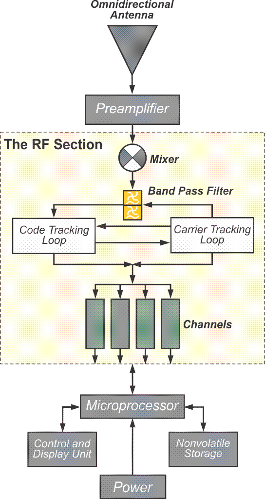
The receivers are the most important hardware in a GPS surveying operation. Their characteristics and capabilities influence the techniques available to the user throughout the work. There are many different GPS receivers on the market. Some of them are appropriate for surveying, and they share some fundamental elements. Though no level of accuracy is ever guaranteed, with proper procedures and data handling they are generally capable of accuracies from sub meter to centimeters. Most are also capable of performing differential GPS, real-time GPS, static GPS, etc., and are usually accompanied by processing and network adjustment software and so on.
GPS receivers come in a variety of shapes and sizes. Some have external batteries, data collectors. Some are tripod mounted. Some are hand-held and have all components built in, and some can be used in both ways, with externals and without. Nevertheless, most have similar characteristics. Here is a schematic drawing of a GPS receiver. It includes some of the common components.

A GPS receiver must collect and then convert signals from GPS satellites into measurements of position, velocity, and time. There is a challenge in that the GPS signal has low power. An orbiting GPS satellite broadcasts its signal across a cone of approximately 28º of arc. From the satellite’s point of view, about 11,000 miles up, that cone covers a substantial portion of the whole planet. It is instructive to contrast this arrangement with a typical communication satellite that not only has much more power, but also broadcasts a very directional signal. Its signals are usually collected by a large dish antenna, but the typical GPS receiver has a small, relatively non-directional antenna. Stated another way, a GPS satellite spreads a low power signal over a large area rather than directing a high power signal at a very specific area. Fortunately, antennas used for GPS receivers do not have to be pointed directly at the signal source. The GPS signal also intentionally occupies a broader bandwidth than it must, to carry its information. This characteristic is used to prevent jamming and mitigate multipath but, most importantly, the GPS signal itself would be completely obscured by the variety of electromagnetic noise that surrounds us if it were not a spread spectrum coded signal. In fact, when a GPS signal reaches a receiver, its power is actually less than the receiver's noise level; fortunately, the receiver can still extract the signal and achieve unambiguous satellite tracking using the correlation techniques described earlier. To do this job, the elements of a GPS receiver function cooperatively and iteratively. That means that the data stream is repeatedly refined by the several components of the device working together as it makes its way through the receiver.
The Antenna and The Right Hand Circular Polarized Signal
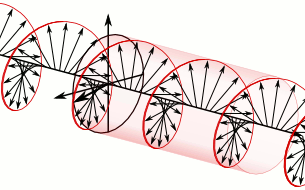
The antenna, radio frequency (RF) section, filtering and intermediate frequency elements are in the front of a GPS receiver. The antenna collects the satellite’s signals and converts the incoming electromagnetic waves into electric currents sensible to the RF section of the receiver. Several antenna designs are possible in GPS, but the satellite’s signal has such a low power density, especially after propagating through the atmosphere, that antenna efficiency is critical. Therefore, GPS antennas must have high sensitivity, also known as high gain. They can be designed to collect only the L1 frequency, L1 and L2, or all signals, including L5. In all cases, they must be Right Hand Circular Polarized, (RHCP), as are the GPS signals broadcast from the satellites.
Polarized waves oscillate in more than one direction. The electrical field vectors of the GPS Signal have a constant magnitude, but their direction rotates so that the electrical field vector of the wave describes a helix in the direction of propagation. Said another way, circularly polarized waves are those where the angle of the electric vector rotates around an imaginary line traveling in the direction of the propagation of the wave. The rotation may be either to the right or left. The GPS signal is a Right-Hand Circularly Polarized (RHCP) wave. You can illustrate it this way. With your right hand, give the thumbs up signal. Now, instead of pointing your thumb up, point it in the direction that the GPS signal is propagating. Your curling fingers show you the direction of the rotation of the field.
The Antenna
Bottom left: Dipole antenna, Bottom right: Helix antenna
Top right: LEA
Bottom left: http://www.sciperio.com/antenna/antenna-design.asp
Bottom right: www.professionalwireless.com/helical/index.aspx
The illustration shows antenna types. They are not specifically GPS antennas.
Most receivers have an antenna built in, but many can accommodate a separate tripod-mounted or range pole-mounted antenna as well. These separate antennas sometimes require connecting coaxial cables. The cables are an important detail. The longer the cable, the more of the GPS signal is lost traveling through it. They are usually in standard lengths to make sure that the impedance of the trip through the cable can be calibrated.
As mentioned earlier, the wavelengths of the GPS carriers are 19 cm (L1), 24 cm (L2) and 25 cm (L5), and antennas that are a quarter or half wavelength tend to be the most practical and efficient, so GPS antenna elements can be as small as 4 or 5 cm. Most of the receiver manufacturers use a microstrip antenna. These are also known as patch antennas. The microstrip may have a patch for each frequency, so it can receive one or all of the GPS carriers. Microstrip antennas are durable, compact, have a simple construction and a low profile. The next most commonly used antenna is known as a dipole. You may recall that this is the kind of antenna that was used with the Macrometer, the first commercial GPS receiver. A dipole antenna has a stable phase center and simple construction, but needs a good ground plane. A ground plane also facilitates the use of a microstrip antenna where it not only ameliorates multipath, but also tends to increase the antenna’s zenith gain-- in other words, the gain of the antenna straight up. A quadrifilar antenna is a single frequency antenna that has two orthogonal bifilar helical loops on a common axis. Quadrifilar antennas perform better than a microstrip on crafts that pitch and roll, like boats and airplanes. They are also used in many recreational handheld GPS receivers. Such antennas have a good gain pattern, do not require a ground plane, but are not azimuthally symmetric. The least common design is the helix antenna. A helix is a dual frequency antenna. It has a good gain pattern, but a high profile.
Bandwidth


An antenna ought to have a bandwidth commensurate with its application. In general, the larger the bandwidth, the better the performance; however, there is downside. Increased bandwidth degrades the signal-to-noise ratio by including more interference. These PSD diagrams illustrate the C/A and P code signals power per bandwidth in Watts per Hertz as a function of frequency. GPS microstrip antennas usually operate in a range from about 2 to 20 MHz, which corresponds with the null-to-null bandwidth of the GPS signals. For example, the L2C signal, like the C/A, has the span of 2.046 megahertz. You can see it in the highest portion or the central lobe of the diagram. L5, like the P code, has a bandwidth of 20.46 megahertz, as you see in red. So an antenna on the front end of the receiver has to be able to accommodate that bandwidth of 20.46 megahertz if it is to track all of these signals. If the system's tracking C/A code or the L2C only, it could have a narrower bandwidth. It would need 2.046 MHz for the central lobe of the C/A code, or if it were designed to track the L1C signal, its bandwidth would need to be 4.092 MHz. A dual frequency microstrip antenna would likely operate in a bandwidth from 10 to 20 MHz.
Nearly Hemispheric Coverage


Since a GPS antenna is designed to be omnidirectional, its gain pattern, that is the change in gain over a range of azimuths and elevations, ought to be nearly a full hemisphere, but not perfectly hemispheric. For example, most surveying applications filter the signals from very low elevations to reduce the effects of multipath and atmospheric delays. A portion of the GPS signal may come into the antenna from below the mask angle; therefore, the antenna’s gain pattern is specifically designed to reject such signals. Second, the contours of equal phase around the antenna’s electronic center, that is, the phase center, are not themselves perfectly spherical.
The gain, or gain pattern, describes the success of a GPS antenna in collecting more energy from above the mask angle, and less from below the mask angle. A gain of about 3 to 5 decibels (dB) is typical for a GPS antenna. Just a brief description of a decibel-- we'll be seeing a little bit more of it. The decibel is a tenth of a bell, which was named for Alexander Graham Bell. It is a logarithmic dimensionless unit used to make a comparison. In this case, the gain of a real GPS antenna is compared to a theoretical lossless antenna that has perfectly equal capabilities in all directions. This imaginary perfection is known as an isotropic antenna. By the way a 3 decibel increase indicates a doubling of signal strength, and a 3 decibel decrease indicates a halving of signal strength so a typical omnidirectional GPS antenna with a gain of about 3 dB (decibels) has about 50% of the capability of that perfect isotropic antenna.
A decibel watt, dbW, indicates the actual power of a signal compared to a reference of one watt, The minimum power received from the C/A code on L1 is about -160dBW, -160 decibel Watts and the minimum power received from the P code on L2 is even less at -166 dBW. It is important that the GPS receiver antennas and pre-amplifiers be as efficient as possible, because the power received from the GPS satellites is low.
Antenna Orientation

In a perfect GPS antenna, the phase center of the gain pattern would be exactly coincident with its actual, physical, center. If such a thing were possible, the centering of the antenna over a point on the earth would ensure its electronic centering as well. But that absolute certainty remains elusive for several reasons.
It is important to remember that the position at each end of a GPS baseline is the position of the phase center of the antenna at each end, not their physical centers, and the phase center is not an immovable point. The location of the phase center actually changes slightly with the satellite’s signal. For example, it is different for the L2 than for L1 or L5. In addition, as the azimuth, intensity, and elevation of the received signal changes, so does the difference between the phase center and the physical center. Small azimuthal effects can also be brought on by the local environment around the antenna. But most phase center variation is attributable to changes in satellite elevation. In the end, the physical center and the phase center of an antenna may be as much as a couple of centimeters from one another. On the other hand, with today’s patch antennas, it can be as little as a few millimeters. It is fortunate that the shifts are systematic. To compensate for some of this offset error, most receiver manufacturers recommend users make sure their antennas are all oriented in the same direction when making simultaneous observations on a network of points. Several manufacturers provide reference marks on the antenna, so that each one may be rotated to the same azimuth, usually north, to maintain the same relative position between their physical and phase, electronic, centers. By orienting all the antennas in the same direction, the offset between the phase center and the physical center is in the same direction at each point. Therefore, the baselines come out exactly as if the physical and the phase center were coincident.
It's only when we're talking about control work, work that needs to be quite accurate, that all of the antennas need to be oriented to the same direction.
Height of Instrument

The antenna's configuration also affects another measurement critical to successful GPS work - the height of the instrument. An incorrect height of instrument is one of the most easily avoided errors. The measurement is normally made to some reference mark on the antenna. In this diagram, you see many ways of measuring that height. It can be measured at slant height or measured with a tape, usually to the antenna reference point. The ARP, or the antenna reference point, is frequently the bottom of the mount of the antenna. There's usually a correction to be added to actually bring that measurement up to the phase center of the antenna. This also becomes part of the necessary information when one is using continuously operating reference stations. We talked earlier about the fact that it is possible to take the downloads from NGS managed Continuously Operating Reference Station (CORS) stations that are available on the Internet and post-process the observations taken with a roving GPS receiver. If you are doing so, it is also necessary to know the height of the antenna at the CORS. Of course, that is not an antenna that you would've set up, but that information is available along with the files from the base station.
The RF Section

The pre-amplifier is necessary, because the signal coming in from the GPS satellite is weak. The preamplifier increases the signal’s power, but it is important that the gain in the signal coming out of the preamplifier is considerably higher than the noise. Noise is always part of the signal. Since signal processing is easier if the signals arriving from the antenna are in a common frequency band, the incoming frequency is combined with a signal at a harmonic frequency. This latter, pure sinusoidal signal is the previously mentioned reference signal generated by the receiver’s oscillator. The two frequencies are multiplied together in a device known as a mixer. Two frequencies emerge: one of them is the sum of the two that went in, and the other is the difference between them. The sum and difference frequencies then go through a bandpass filter, an electronic filter that removes the unwanted high frequencies and selects the lower of the two. It also eliminates some of the noise from the signal. For tracking the P(Y)-code, this filter will have a bandwidth of about 20 MHz, but it will be around 2 MHz if the C/A code is required. In any case, the signal that results is known as the intermediate frequency (IF), or beat frequency signal. This beat frequency is the difference between the Doppler-shifted carrier frequency that came from the satellite and the frequency generated by the receiver’s own oscillator. In fact, to make sure that it embraces the full range of the Doppler effect on the signals coming in from the GPS satellites, the bandwidth of the IF itself can vary from 5 to 10 kHz Doppler. That spread is typically lessened after tracking is achieved.


As mentioned before, a replica of the C/A or P(Y) code is generated by the receiver’s oscillator and that is correlated with the IF signal. It is at this point that the pseudorange is measured. Remember, the pseudorange is the time shift required to align the internally generated code with the IF signal, multiplied by the speed of light. The receiver also generates another replica, this time a replica of the carrier. That carrier is correlated with the IF signal and the shift in phase can be measured. The continuous phase observable, or observed cycle count, is obtained by counting the elapsed cycles since lock-on and by measuring the fractional part of the phase of the receiver generated carrier.
Channels

We're not talking about just receiving one signal from one satellite but rather a minimum of four, and perhaps many more, from four to more satellites and the antenna itself does not sort the information it gathers. The signals from several satellites enter the receiver simultaneously. But in the channels of the RF section, the undifferentiated signals are identified and segregated from one another. There are usually several IF stages before the copies are sent into the separate channels, each of which extract the code and carrier information from a particular satellite. A channel in a continuous tracking GPS receiver is not unlike a channel in a television set. It is hardware, or a combination of hardware and software, designed to separate one signal from all the others. A receiver may have 6 channels, 12 channels, or hundreds of channels. At any given moment, one frequency from one satellite can have its own dedicated channel, and the channels operate in parallel. This approach allows the receiver to maintain accuracy when it is on a moving platform; it provides anti-jamming capability and shortens the time to first fix (TTFF). Each channel typically operates in one of two ways; working to acquire the signal or to track it. Once the signal is acquired, it is continuously tracked unless lock is lost. If that happens, the channel goes back to acquisition mode and the process is repeated.
While a parallel receiver has dedicated separate channels to receive the signals from each satellite that it needs for a solution, a multiplexing (aka muxing) receiver gathers some data from one satellite and then switches to another satellite and gathers more data and so on. Such a receiver can usually perform this switching quickly enough that it appears to be tracking all of the satellites simultaneously. A multiplexing receiver must still dedicate one frequency from one satellite to one channel at a time; it just makes that time very short. It typically switches at a rapid pace, i.e., 50 Hz. Even though multiplexing is generally less expensive, this strategy of switching channels is now little used. There are several reasons. While a parallel receiver does not necessarily offer more accurate results, parallel receivers with dedicated channels are faster; a parallel receiver has a more certain phase lock; and there is redundancy if a channel fails and they possess a superior signal-to-noise ratio (SNR). A multiplexing receiver also has a lower resistance to jamming and interference compared to continuous tracking receivers. Whether continuous or switching channels are used, a receiver must be able to discriminate between the incoming signals. They may be differentiated by their unique C/A codes on L1, their Doppler shifts, or some other method, but, in the end, each signal is assigned to its own channel.
Tracking Loops

There are code tracking loops, the delay lock loops (DLL) and carrier tracking loops, and the phase locking loops (PLL) in the receiver. Typically, both the code and the carrier are being tracked in phase lock. The tracking loops connected to each of the receiver’s channels also work cooperatively with each other. As mentioned, dual frequency receivers have dedicated channels and tracking loops for each frequency.
Pseudoranging
In most receivers, the first procedure in processing an incoming satellite signal is synchronization of the C/A code from the satellite’s L1 broadcast, with a replica C/A code generated by the receiver itself, i.e., the code-phase measurement. When there is no initial match between the satellite’s code and the receiver’s replica, the receiver time shifts, or slews, the code it is generating until the optimum correlation is found. Then a code tracking loop, the delay lock loop, keeps them aligned. The time shift discovered in that process is a measure of the signal’s travel time from the satellite to the phase center of the receiver’s antenna. Multiplying this time delay by the speed of light gives a range. But it is called a pseudorange in recognition of the fact that it is contaminated by the errors and biases set out in Lesson 2. The tracking loops that we see in the schematic diagram at the top are the code tracking loops.
Tracking loops are connected to each of the receiver's channels and also work cooperatively with each other. Multiple frequency receivers have dedicated channels and tracking loops for each frequency. Most receivers use the pseudorange range (the C/A code, on the L1) as the front door, so to speak, for the incoming satellite's synchronization. As we've discussed, the replica code is used to accomplish correlation. As you see in the diagram, the incoming signal is in the green at the top. The receiver replica is in blue. There is illustration of the replica as early, prompt, and late. When it is prompt, the replica and the incoming signal are correlated.
Carrier Phase Measurement
Once the receiver acquires the C/A code, it has access to the NAV message, or the newer navigation messages such as CNAV. It can read the ephemeris and the almanac information, use GPS time. But the code’s pseudoranges, alone, are not adequate for the majority of applications. Therefore, the next step in signal processing for most receivers involves the carrier phase observable. As stated earlier, just as they produce a replica of the incoming code, receivers also produce a replica of the incoming carrier wave. And the foundation of carrier phase measurement is the combination of these two frequencies. Remember, the incoming signal from the satellite is subject to an ever-changing Doppler shift, while the replica within the receiver is nominally constant.
Carrier Tracking Loop
The process begins after the PRN code has done its job and the code tracking loop is locked. By mixing the satellite’s signal with the replica carrier, this process eliminates all the phase modulations, strips the codes from the incoming carrier, and simultaneously creates two intermediate or beat-frequencies—one is the sum of the combined frequencies, and the other is the difference. The receiver selects the latter, the difference, with a bandpass filter. Then, this signal is sent on to the carrier tracking loop also known as the phase locking loop, PLL, where the voltage-controlled oscillator is continuously adjusted to follow the beat frequency exactly. This is basically how a GPS receiver locks on to that carrier and stays locked unless there is a loss of signal or a cycle slip.
Doppler Shift

We've talked about the Doppler shift in several different contexts. One was the original transit system, NNSS system, that operated on the Doppler shift. As the satellite passes overhead, the range between the receiver and the satellite changes; that steady change is reflected in a smooth and continuous movement of the phase of the signal coming into the receiver. GPS uses the Doppler shift as an observable. It has broad applications in signal processing. It can be used to discriminate between the signals from various GPS satellites, to determine integer ambiguities in kinematic surveying, as a help in the detection of cycle slips, and as an additional independent observable for autonomous point positioning. But perhaps the most important application of Doppler data is the determination of the range rate between a receiver and a satellite. Range rate is a term used to mean the rate at which the range between a satellite and a receiver changes over a particular period of time.
Typical Change in the Doppler Shift
This graphic shows the typical rate of change in the Doppler shift with regard to a stationary, static, GPS receiver. The signal received would have its maximum Doppler shift, +4 1/2 to 5 cycles per millisecond, when the satellite is at its maximum range, just as it is rising or setting. The Doppler shift continuously changes throughout the overhead pass. Immediately after the satellite rises, relative to a particular receiver, its Doppler shift gets smaller and smaller, until the satellite reaches its closest approach, at zenith. At that moment its radial velocity with respect to the receiver is zero, the Doppler shift of the signal is zero as well. But as the satellite recedes, it grows again, negatively, until the Doppler shift once again reaches its maximum extent just as the satellite sets, -4 1/2 to 5 cycles per millisecond. It is very predictable. That predictability, the constant variation of the signal's Doppler shift, makes it a good observable. If the receiver's oscillator frequency is adjusted to match these variations exactly, as they're happening, it will duplicate the incoming signal's shift and phase. This strategy of making measurements using the carrier beat phase observable is a matter of counting the elapsed cycles and adding the fractional phase of the receiver's own oscillator. This is one way that the phase lock loop maintains its lock on the signal as the Doppler shift occurs with each of the satellites that it is tracking.
With respect to the receiver, the satellite is always in motion even if the receiver is static. But the receiver may be in motion in another sense, as it is in kinematic GPS. The ability to determine the instantaneous velocity of a moving vehicle has always been a primary application of GPS, and is based on the fact that the Doppler-shift frequency of a satellite’s signal is nearly proportional to its range rate. The Doppler shift can be used to discriminate between the signals of the various satellites to help in the determination of the integer ambiguity. It can help in detection of a loss of lock due to a cycle slip.
Continuously Integrated Doppler
The Doppler-shift and the carrier phase are measured by first combining the received frequencies with the nominally constant reference frequency created by the receiver’s oscillator. The difference between the two is the often mentioned beat frequency, an intermediate frequency, and the number of beats over a given time interval is known as the Doppler count for that interval. Since the beats can be counted much more precisely than their continuously changing frequency can be measured, most GPS receivers just keep track of the accumulated cycles, the Doppler count. The sum of consecutive Doppler counts from an entire satellite pass is often stored, and the data can then be treated like a sequential series of biased range differences. Continuously Integrated Doppler is such a process. The rate of the change in the continuously integrated Doppler shift of the incoming signal is the same as that of the reconstructed carrier phase. Integration of the Doppler frequency offset results in an accurate measurement of the advance in carrier phase between epochs. And as stated earlier, using double-differences in processing the carrier phase observables removes most of the error sources other than multipath and receiver noise.
The Integer Ambiguity

The solution of the integer ambiguity, the number of whole cycles on the path from satellite to receiver, would be more difficult if it was not preceded by pseudoranges, or code phase measurements in most receivers. This allows the centering of the subsequent double-difference solution. In other words, a pseudorange solution provides an initial estimate of the candidates for the integer ambiguity within a smaller range than would otherwise be the case, and, as more measurements become available, it can reduce them even further. After the code-phase measurements narrows the field, there are several methods used to solve the integer ambiguity. In the geometric method, the carrier phase data from multiple epochs are processed, and the constantly changing satellite geometry is used to find an estimate of the actual position of the receiver. This approach is also used to show the error in the estimate by calculating how its results hold up as the geometry of the constellation changes. This strategy requires a significant amount of satellite motion to succeed, and, therefore, takes time to converge on a solution. It works pretty well, but requires satellite motion and takes time to converge. Another approach to solving the integer ambiguity is filtering. Independent measurements are averaged to find the estimated position with the lowest noise level. A third uses a search through the range of possible integer ambiguity combinations from which it calculates the one with the lowest residuals. These approaches can't assess the correctness of the particular answer, but they can provide the probability with certain conditions, that the answer is within given limits. Most GPS receivers use a combination of methods. Nearly all narrow the field by beginning with an initial position established by the code phase measurements. They then use one or more of the methods in combination to come up with the most probable value for the solution of the integer ambiguity, the N, the number of full wave cycles between the receiver and the satellite at lock on, the key to carrier phase observations.
Signal Squaring
There is a method that does not use the codes carried by the satellite’s signal. It is called codeless tracking, or signal squaring. It was first used in the earliest civilian GPS receivers, supplanting proposals for a TRANSIT-like Doppler solution. It makes no use of pseudoranging and relies exclusively on the carrier phase observable. Like other methods, it also depends on the creation of an intermediate or beat frequency. But with signal squaring, the beat frequency is created by multiplying the incoming carrier by itself. The result has double the frequency and half the wavelength of the original. It is squared. There are some drawbacks to the method. For example, in the process of squaring the carrier, it is stripped of all its codes. The chips of the P(Y) code, the C/A code, and the Navigation message normally modulated onto the carrier by 180° phase shifts are eliminated entirely. As discussed earlier, the signals broadcast by the satellites have phase shifts called code states that change from +1 to –1 and vice versa, but squaring the carrier converts them all to exactly 1. The result is that the codes themselves are wiped out. Therefore, this method must acquire information such as almanac data and clock corrections from other sources. Other drawbacks of squaring the carrier include the deterioration of the signal-to-noise ratio, because when the carrier is squared, the background noise is squared, too. And cycle slips occur at twice the original carrier frequency. But signal squaring has its up-side as well. It reduces susceptibility to multipath. It has no dependence on PRN codes and is not hindered by the encryption of the P code. The technique works as well on L2 as it does on L1 or L5, and that facilitates ionospheric delay correction. Therefore, signal squaring can provide high accuracy over long baselines. So, there is a cursory look at some of the different techniques used to process the signal in the RF section. Now let's look at the microprocessor of the receiver.
The Microprocessor

The microprocessor in a GPS receiver is the computer that manages data collection and is the home of the applications that mitigate multipath, noise, extract the ephemerides and other information from the Navigation message or newer navigation messages such as CNAV. It controls the entire receiver: the digital circuits, the tracking, and measurements. The receiver also has storage. However, more and more, the microprocessor is expected to produce the position in real time, instantaneously, or near real-time by processing the ranging data, doing reference frame (datum) conversion, and sending the position to the control and display unit (CDU). There is a two-way street between the microprocessor and the CDU; each can receive information from or send information to the other.
Differential Positioning
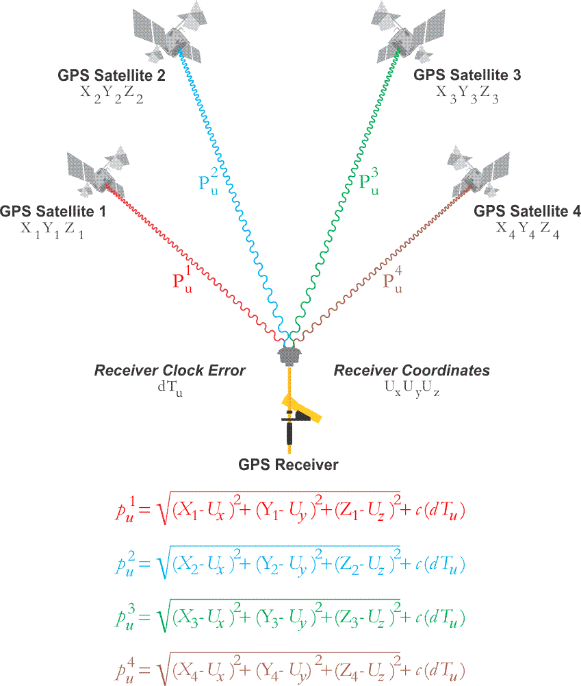
Autonomous single-point positioning using unsmoothed code pseudoranges are based upon corrections provided in the navigation messages, which, as you know, have a certain amount of weakness. Though they have improved since Selective Availability has been switched off, they are generally not as accurate as differentially corrected positions. Code-based pseudoranges using DGPS, differential GPS, can achieve good real-time, or post-processed results. DGPS is often used in collecting data for Geographical Information Systems, GIS.
DGPS

The type of differential positioning sometimes known as DGPS depends on code pseudorange observations, but requires at least two receivers. One receiver is placed on a control station, the base, and another on an unknown position, the rover. The base station antenna needn't be on a building, as illustrated. It could be on a tower. It could be on a non-GPS satellite. There are services that allow you to subscribe to a correction signal. In those cases, there is a network of base stations collecting the signals from the constellation; the correction signal is compiled, beamed up to the non-GPS satellite, and that same message sent back down from the non-GPS satellite to subscribers. In all configurations, the base and the rover simultaneously receive the same signals from the same constellation of at least four GPS/GNSS satellites. That's important in that the way many of the errors in the observations are common to both the base and the rover receivers, the errors are correlated and tend to cancel each other to some degree. The data from such an arrangement can be post-processed; although, with a link between the base and the rover, a correction signal can be sent to the rover so that differential results can be had in real-time. Improvements in this technology have refined the technique's accuracy markedly, and meter- or even submeter results are possible. Still, the positions are not as reliable as those achieved with the carrier phase observable.
With GIS, corner search and mapping work excepted, much GPS work requires a higher standard of accuracy. Certainly, GPS control surveying often employs several static receivers that simultaneously collect and store carrier phase data from the same satellites for a period of time known as a session. After all the sessions for a day are completed, their data are usually downloaded in a general binary format to the hard disk of a PC for post-processing. However, carrier phase positioning can also be done in real-time.
Real-Time Kinematic

Real-time kinematic surveying uses the carrier phase solution. Often, there is a radio link between the base and rover. While the baseline length with DGPS is often 100 to 200 kilometers or longer, the baseline length in RTK is more typically 10 to 20 kilometers, often less. However, the arrangement of receivers is similar: the constellation of satellites being tracked at the base station and also tracked at the rover, the base station is at a known point. There is a transmission antenna used in RTK. It transmits the correction signals to the rover in real time correction. While the arrangement is similar to DGPS, the solution is carrier phase as opposed to pseudorange. The minimum number of satellites with RTK is five. It is five, so that one can be lost and still assured that there will be a solution.
The CDU

A GPS receiver will often have a control and display unit. From handheld keyboards to soft keys around a screen to digital map displays and interfaces to other instrumentation, there are a variety of configurations. Nevertheless, they all have the same fundamental purpose, facilitation of the interaction between the operator and the receiver’s microprocessor. A CDU typically displays status, position data, velocity, and time. It may also be used to select different surveying methods, waypoint navigation, and/or set parameters such as epoch interval, mask angle, and antenna height. The CDU can offer a combination of help menus, prompts, reference frame (datum) conversions, readouts of survey results, estimated positional error, and so forth. The information available from the CDU varies from receiver to receiver. But when four or more satellites are available, they can generally be expected to display the PRN numbers of the satellites being tracked, the receiver’s position in three dimensions, and velocity information. Most of them also display the dilution of precision and GPS time or UTC.
The Storage


Most GPS receivers today have internal data logging. The amount of storage required for a particular session depends on several things: the length of the session, the number of satellites above the horizon, the epoch interval, and so forth. For example, presuming the amount of data received from a single GPS satellite is ~100 bytes per epoch, a typical twelve channel dual-frequency receiver observing 6 satellites and using a 1-second epoch interval over the course of a 1-hour session would require ~2MB of storage capacity for that session. The miniaturization of storage continues. The cassettes, floppy disks, and drives used with the Macrometer are past. Extraordinary amounts of data can be stored in small, convenient devices or sent to the cloud.
The Power
Battery power

It is fortunate that GPS receivers operate at low power. From 9 to 36 volts DC is generally required. This allows longer observations with fewer, and lighter, batteries than might be otherwise required. It also increases the longevity of the GPS receivers, themselves. About half of the available GPS carrier phase receivers have an internal power supply, and most will operate 5½ hours or longer on a fully charged 6-amp-hour battery. Most code-tracking receivers, those that do not also use the carrier phase observable, could operate for about 15 hours on the same size battery. Since most receivers in the field operate on battery power, batteries and their characteristics are fundamental to GPS/GNSS. A variety of batteries are used, and there are various configurations. For example, some units are powered by rechargeable batteries. Lithium, Nickel Cadmium, and Nickel Metal-Hydride may be the most common categories, but lead-acid car batteries still have an application as well. The obvious drawbacks to lead-acid batteries are size and weight. And there are a few others—the corrosive acid, the need to store them charged, and their low cycle life. Nevertheless, lead-acid batteries are especially hard to beat when high power is required. They are economical and long-lasting.
Nickel Cadmium batteries (NiCd) cost more than lead-acid batteries, but are small and operate well at low temperatures. Their capacity does decline as the temperature drops. Like lead-acid batteries, NiCd batteries are quite toxic. They self-discharge at the rate of about 10% per month, and even though they do require periodic full discharge, these batteries have an excellent cycle life. Nickel Metal-Hydride (NiMH) batteries self-discharge a bit more rapidly than NiCd batteries and have a less robust cycle life, but are not as toxic. Lithium–ion batteries overcome several of the limitations of the others. They have a relatively low self-discharge rate. They do not require periodic discharging and do not have a memory issues as do NiCd batteries. They are light, have a good cycle life and low toxicity. On the other hand, the others tolerate overcharging, and the lithium-ion battery does not. It is best to not charge lithium-ion batteries at temperatures at or below freezing. These batteries require a protection circuit to limit current and voltage, but are widely used in powering electronic devices, including GPS/GNSS receivers.
Some GPS Surveying Methods

Static GPS surveying was the first method of GPS surveying used in the field, and it continues to be the primary technique for GPS/GNSS control today. Relative static positioning involves several stationary receivers simultaneously collecting data from at least four satellites during observation sessions that usually last from 30 minutes to 2 hours. A typical application of this method would be the determination of vectors, or baselines as they are called, between several static receivers to accuracies from 1 ppm to 0.1 ppm over tens of kilometers. There are few absolute requirements for relative static positioning. The requisites include: more than one receiver, four or more satellites, and a mostly unobstructed sky above the stations to be occupied. But, as in most of surveying, the rest of the elements of the system are dependent on several other considerations.

Here is a diagram of approximate session lengths required for GPS static surveying. For example, with an eight satellite constellation and a 10 kilometer baseline, something between a half an hour and an hour would typically be required. A four satellite constellation might require a session between one and two hours for a baseline of the same length. The assessment of the productivity of a GPS survey almost always hinges, in part at least, on the length of the observation sessions required to satisfy the survey specifications. The determination of the session's duration depends on several particulars, such as the length of the baseline and the relative position, that is the geometry, of the satellites among others. Generally speaking, the larger the constellation of satellites, the better the available geometry, the lower the positioning dilution of precision (PDOP), and the shorter the length of the session needed to achieve the required accuracy. For example, given six satellites and good geometry, baselines of 10 km or less might require a session of 45 minutes to 1 hour, whereas, under exactly the same conditions, baselines over 20 km might require a session of 2 hours or more. Alternatively, 45 minutes of six-satellite data may be worth an hour of four-satellite data, depending on the arrangement of the satellites in the sky.
Relative static positioning, just as all the subsequent surveying methods discussed here, involves several receivers occupying many sites. Problems can be avoided as long as the receivers on a project are compatible. For example, it is helpful if they have the same number of channels and signal processing techniques. The subject comes up from time to time as to whether or not data from receivers from various manufacture can be used on the same project together at the ends of even the same baseline. The answer is, yes of course because fortunately, there is a file format, that allows one to use receivers of many types together. It is the Receiver Independent Exchange Format, RINEX , developed by the Astronomical Institute of the University of Berne in 1989. It allows different receivers and post-processing software to work together. Almost all GPS/GNSS processing software will output RINEX files.
Receiver Categories
- Recreation Receivers
- Mapping Receivers
- Surveying Receivers

Receivers are generally categorized by their physical characteristics, the elements of the GPS signal they can use with advantage, and by the claims about their accuracy. There are receivers that use only the C/A code on the L1 frequency and receivers that cross-correlate with the P(Y) There are L1 carrier phase tracking receivers, dual-frequency and multi-frequency carrier phase tracking receivers, receivers that track all in view, and GPS/GNSS receivers. The more aspects of the GPS signal a receiver can employ, the greater its flexibility, but so, too, the greater its cost. It is important to understand receiver capabilities and limitations to ensure that the systematic capability of a receiver is matched to the required outcome of a project. As shown in the illustration, it is possible to divide receivers into three categories. They are; recreation, mapping, and surveying.
Recreational Receivers
| Recreational receivers | Autonomous Horizontal Precision |
Real-time Corrected Horizontal Network Accuracy |
Post-processed Horizontal Network Accuracy |
|---|---|---|---|
| Recreation | 5 - 15 m | 2 - 5 m | 5 - 15 m |
Recreation Receivers
These receivers are generally defined as L1 Code receivers which are typically not user configurable for settings such as mask angle, PDOP, the rate at which measurements are downloaded, the logging rate, also known as the epoch interval, and signal to noise ratio SNR. As you might expect, SNR is the ratio of the received signal power to the noise floor of a GPS observation. It is typical for the antenna, receiver, and CDU to be integrated into the device in these receivers. Generally speaking, receivers that track the C/A code provide only relatively low accuracy. Most are not capable of tracking the carrier phase observable. These receivers were typically developed with basic navigation in mind. Most are designed for autonomous (stand-alone) operation to navigate, record tracks, waypoints, and routes aided by the display of onboard maps. They are sometimes categorized by the number of waypoints they can store. Waypoint is a term that grew out of military usage. It means the coordinate of an intermediate position a person, vehicle, or airplane must pass to reach a desired destination. With such a receiver, a user may call up a distance and direction from his present location to the next waypoint.
A single receiver operating without augmentation produces positions which are not relative to any ground control, local or national. In that context, it is more appropriate to discuss the precision of the results than it is to discuss accuracy. Despite the limitations, some recreational receivers have capabilities that enhance their systematic precision and achieve a quantifiable accuracy using correction signals available from earth-orbiting satellites such as the Wide Area Augmentation System, WAAS correction. In other words, some have differential capability. The Wide Area Augmentation System is a U.S. Federal Aviation Authority FAA and the U.S. Department of Transportation DOT system that augments GPS accuracy, availability, and integrity. The system relies on a network of ground-based reference stations at known positions that observe the GPS constellation constantly. From their data, a correction message is calculated at two master stations. This message is uploaded to satellites on geostationary orbits. The satellites broadcast the message, and WAAS-enabled receivers can collect it and use the correction provided in it. For example, it provides a correction signal for precision approach aircraft navigation. Similar systems are Europe’s European Geostationary Navigation Overlay System, EGNOS, and Japan’s Multifunction Transport Satellite, MTSAT.
Recreational grade receivers typically do not have on-board feature data collection capabilities. They also do not usually have adequate on-board storage for recording the features (coordinates and attributes) required for a mapping project. Such capabilities are not needed for their designed applications. When a recreation receiver is used to obtain an autonomous, or stand alone, position, its precision may be within a range of 5-15m, as noted in Table 4.1. Under less than optimal field conditions: tree cover and other obstructions, less than favorable GPS satellite geometry, etc., users can expect the precision of autonomous positions to lessen, sometimes substantially. The network accuracy had with real-time differential correction of 2-5m is also not always achievable due to the tendency of the Wide Area Augmentation Signal being difficult to acquire, particularly in the northern US and then only with a southern sky clear of obstruction.
Local and Network Accuracy

Local and Network Accuracy
The use of the phrase network accuracy is used to define its difference from local accuracy. Network accuracy, here, concerns the uncertainty of a position relative to a reference frame (datum). Local accuracy is not about a position relative to a reference frame (datum), but it represents the uncertainty of a position relative to other positions nearby. In other words, local accuracy would be useful in knowing the accuracy of a line between the two positions at each end. Network accuracy would not be about the accuracy of the positions at each end of the line relative to each other, but, rather, relative to the whole reference frame (datum). Local Accuracy is also known as relative accuracy, and network accuracy is also known as absolute accuracy.
Within a well-defined geographical area, local accuracy may be the most immediate concern. However, those tasked with constructing a control network that embraces a wide geographical scope will most often need to know the position's relationship to the realization of the reference frame (datum) on which they are working. A point with good local accuracy may not have good network accuracy. Typically, network horizontal and vertical accuracies require that a point's accuracy be specified with respect to an appropriate national geodetic datum. In the United States, as a practical matter, this most often means that the work is tied to at least one of the Continuously Operating Reference Stations (CORS) which represent the most accessible realization of the National Spatial Reference System (NSRS) in the nation.
Mapping Receivers
| Mapping Receivers | Autonomous Horizontal Precision |
Real-time Corrected Horizontal Network Accuracy |
Post-processed Horizontal Network Accuracy |
|---|---|---|---|
| Mapping (L1 Code) | 2 - 10m | 0.5 - 5m | 0.3 - 15m |
| Mapping (L1 Code & Carrier) | 2 - 10m | 0.5 - 3m | 0.2 - 1m |
| Mapping (All GPS Code & Carrier) | 2 - 10m | 0.5 - 3m | 0.02 - 0.9m |
| Mapping (GNSS) | 2 - 10m | 0.5 - 3m | 0.02 - 0.9m |
Mapping Receivers
These receivers are generally defined as those that allow the user to configure some settings such as PDOP, SNR (carrier-to-noise-density ratio C/N0), elevation mask and the logging rate. They most often have an integrated antenna and CDU in the receiver. They generally record pseudoranges and also can log data suitable for differential corrections either in real-time or for post-processing; many record carrier data. Mapping receivers are often capable of storing mapped features (coordinates and attributes) and usually have adequate capacity for mapping applications. This memory is required for differential GPS, DGPS receivers, even those that track only code. For many applications, a receiver must be capable of collecting the same information as is simultaneously collected at a base station, and storing it for post-processing. Receivers typically depend on proprietary post-processing software, which also includes utilities to enable GPS data to be transferred to a PC and exported in standard GIS file format(s) either over a cable or a wireless connection. Some mapping grade receivers for spatial data collection are single frequency with code only or both code and carrier. Most mapping grade receivers of all tracking configurations are WAAS (or other Satellite Based Augmentation Signal SBAS) enabled, and thereby offer real-time results. Such differentially corrected mapping receivers may be capable of achieving a network accuracy of ~0.5 to 5 meters. Positions of sub-meter post-processed network accuracy can be achieved with mapping grade receivers. As noted, some mapping receivers offer tracking of the Global Navigation Satellite System, GNSS, constellations.
GNSS

Click here to see a text description.
GNSS
As mentioned earlier, the Global Positioning System (GPS) is now a part of a growing international context—the Global Navigation Satellite System (GNSS). One definition of GNSS embraces any constellation of satellites providing signals from space that facilitate autonomous positioning, navigation, and timing on a global scale. Currently, there are four systems that satisfy this definition. It is the Russian Federation’s GLONASS, European Union's GALILEO, China's BEIDOU and America's GPS.
There are several other regional satellite position, navigation and timing systems such as the Indian Regional Navigation Satellite System (IRNSS) and the Japanese Quasi-Zenith Satellite System (QZSS).
Surveying Receivers
| Survey Receivers | Autonomous Horizontal Precision |
Real-time Corrected Horizontal Network Accuracy |
Post-processed Horizontal Network Accuracy |
|---|---|---|---|
| Survey | 2 - 10 m | > 1 m | > 0.1 m |
Surveying Receivers
Survey grade receivers are designed for the achievement of consistent network accuracy in the static or real-time mode. Positions determined by these receivers will generally provide the best accuracy of the categories listed. The components of these receivers can usually be configured in a variety of ways. The receivers are typically multi-frequency, code and carrier receivers. Many are GNSS receivers. They generally provide more options for setting the observational parameters than recreational or mapping receivers. Surveying receivers are typically capable of observing the civilian code and carrier phase of all frequencies, and are appropriate for collecting positions on long baselines. Survey grade receivers are capable of producing network accuracies of better than 1 m with real-time differential correction and better than 0.1 m with post-processing.
Most share some practical characteristics: they have multiple independent channels that track the satellites continuously, and they begin acquiring satellites’ signals from a few seconds to less than a minute from the moment they are switched on. Most acquire all the satellites above their mask angle in a very few minutes, with the time usually lessened by a warm start, and most provide some sort of alert to the user that data is being recorded, and so forth. About three-quarters of them can have their sessions preprogrammed in the office before going to their field sites. Nearly all allow the user to select the logging rate, also known as epoch interval and also known as sampling interval. While a 1 second interval is often used, faster rates of 0.1 second (10 Hz) and more increments of tenths of a second are often available. This feature allows the user to stipulate the short period of time between each of the microprocessor's downloads to storage. The faster the data-sampling rate, the larger the volume of data a receiver collects, and the larger the amount of storage it needs. A fast rate is helpful in cycle slip detection, and that improves the receiver’s performance on baselines longer than 50 km, where the detection and repair of cycle slips can be particularly difficult.
Discussion
Discussion Instructions
To continue the discussion begun by this lesson, I would like to pose this question:
What are differences between differential GPS, static or kinematic, and autonomous (non-differential) GPS? Does differential GPS have to be post-processed?
To participate in the discussion, please go to the Lesson 4 Discussion Forum in Canvas. (That forum can be accessed at any time by going to the GEOG 862 course in Canvas and then looking inside the Lesson 4 module.)
Summary
The receivers and methods of GPS are constantly evolving and changing. There are, nevertheless, some well established principles. Some of those have been explained in this lesson.
There is another principle. GPS/GNSS is a geodetic system. It is not possible to understand it without some understanding of geodesy - the subject of the next lesson. As a matter of fact, it isn’t hard to operate a GPS/GNSS receiver - most of them are so user-friendly you don’t need to know the first thing about GPS/GNSS to make them work, that is, until they don’t.
Getting coordinates from a GPS/GNSS receiver is usually a matter of pushing a few buttons, but knowing what those coordinates are, and more importantly, what they aren’t, is more difficult. It is vital to have an idea of how the values were measured; otherwise you are at the mercy of the black box, and since it doesn’t always tell the truth, that’s not a good idea.
Before you go on to Lesson 5, double-check the Lesson 4 Checklist to make sure you have completed all of the activities listed there.
Lesson 5: Geodetic Datums
The links below provide an outline of the material for this lesson. Be sure to carefully read through the entire lesson before returning to Canvas to submit your assignments.
Lesson 5 Overview
Overview
Despite the certainty of the physical surface of the Earth, it remains notoriously difficult to define in mathematical terms. The dilemma is illustrated by the ancient struggle to represent its curved surface on flat maps. There have been a whole variety of map projections developed over the centuries that rely on mathematical relationships between positions on the Earth's surface and points on the map. Each projection serves a particular application well, but none of them can represent the Earth without distortion.
As the technology of measurement has improved, the pressure for greater exactness in the definition of the Earth's shape has increased.
Plane surveying has traditionally relied on an imaginary flat reference surface, or reference frame (datum), with Cartesian axes. This rectangular system is used to describe measured positions by ordered pairs, usually expressed in northings and eastings, or y- and x- coordinates. Even though we have always known that this assumption of a flat earth is fundamentally unrealistic, it provided, and continues to provide, an adequate arrangement for small areas. The attachment of elevations to such horizontal coordinates somewhat acknowledges the topographic irregularity of the earth, but the whole system is always undone by its inherent inaccuracy as the area grow large. Even with electronic tools that widen the scope and increase the precision of the data, perfection is nowhere in sight.
The next lesson concerns some of the elements of the systems we inevitably use to accommodate the vagaries of assigning coordinates to the results of an earth-centered-earth-fixed positioning system based on signals from satellites.
Objectives
At the successful completion of this lesson, students should be able to:
- demonstrate understanding of the basics of geodetic coordinates;
- describe a few pertinent ideas about geodetic datums;
- describe plane surveying;
- recognize the structure of some geodetic coordinate systems;
- define the elements of a geodetic datum;
- discuss the geoid; and
- explain the North American Datum 1983.
Questions?
If you have any questions now or at any point during this week, please feel free to post them to the Lesson 5 Discussion Forum. (To access the forum, return to Canvas and navigate to the Lesson 5 Discussion Forum in the Lesson 5 module.) While you are there, feel free to post your own responses if you, too, are able to help out a classmate.
Checklist
Lesson 5 is one week in length. (See the Calendar in Canvas for specific due dates.) To finish this lesson, you must complete the activities listed below. You may find it useful to print this page out first so that you can follow along with the directions.
| Step | Activity | Access/Directions |
|---|---|---|
| 1 | Read the lesson Overview and Checklist. | You are in the Lesson 5 online content now. The Overview page is previous to this page, and you are on the Checklist page right now. |
| 2 | Read "A Few Pertinent Ideas about Geodetic Datums for GPS" in Chapter 5 pages 129 to 141 in GPS for Land Surveyors | Text |
| 3 | Read the lecture material for this lesson. | You are currently on the Checklist page. Click on the links at the bottom of the page to continue to the next page, to return to the previous page, or to go to the top of the lesson. You can also navigate the lecture material via the links in the Lessons menu. |
| 4 | Participate in the Discussion. | To participate in the discussion, please go to the Lesson 5 Discussion Forum in Canvas. (That forum can be accessed at any time by going to the GEOG 862 course in Canvas and then looking inside the Lesson 5 module.) |
| 5 | Read lesson Summary. | You are in the Lesson 5 online content now. Click on the "Next Page" link to access the Summary. |
GPS/GNSS and Geodesy
Hello! And welcome to Lesson Five in the course. This lesson will be about geodetic reference frames (datums), because it is not possible to use GPS/GNSS without engaging in geodesy.
Therefore, it is necessary to understand the native format of GPS/GNSS coordinates, and how the elements of geodesy influence those coordinates. Geodesy is a complicated subject, but we will be talking about just a few elements of the science.
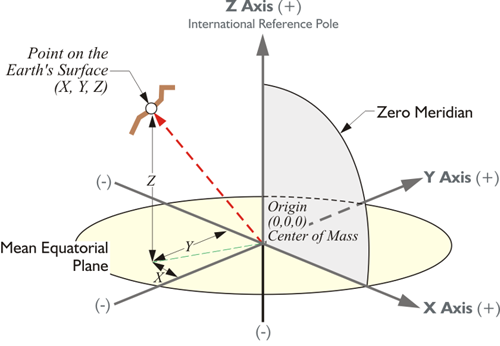
GPS/GNSS and Geodesy
Today, GPS/GNSS has thrust us into the thick of geodesy, which is no longer the exclusive realm of distant experts. Thankfully, in the age of the microcomputer, the computational drudgery can be handled with software packages. Nevertheless, it is unwise to venture into GPS/GNSS believing that knowledge of the basics of geodesy is, therefore, unnecessary. It is true that GPS/GNSS would be impossible without computers, but blind reliance on the data they generate eventually leads to disaster.
Some Geodetic Coordinate Systems
Three-Dimensional (3-D) Cartesian Coordinates
A spatial Cartesian system with three axes lends itself to describing the terrestrial positions derived from space-based geodesy. Using three rectangular coordinates instead of two, one can unambiguously define any position on the Earth, or above it for that matter. The three-dimensional Cartesian coordinates (x,y,z) derived from this system are known as Earth-Centered-Earth-Fixed (ECEF) coordinates. It is a right-handed orthogonal system that rotates with and is attached to the Earth, which is why it is called Earth fixed.
A three-dimensional Cartesian coordinate system is right-handed if it can be described by the following model: the extended forefinger of the right hand symbolizes the positive direction of the x-axis. The middle finger of the same hand extended at right angles to the forefinger symbolizes the positive direction of the y-axis. The extended thumb of the right hand, perpendicular to them both, symbolizes the positive direction of the z-axis.

But such a system is only useful if its origin (0,0,0) and its axes (x,y,z) can be fixed to the planet with certainty, something easier said than done.
This illustration shows the three-dimensional Cartesian coordinate system. It is possible to express a point on the Earth's surface in terms of these x, y, and z-coordinates in this Earth-Centered, Earth-Fixed, or ECEF system. This is the native system in which GPS/GNSS coordinates are expressed; obviously, the plane of the equator, the mean equatorial plane, and the zero meridian (aka Prime Meridian), are vital elements of this system. The usual arrangement is known as the Conventional Terrestrial Reference System (CTRS), and the Conventional Terrestrial System (CTS). The latter name will be used here. The origin is the center of mass of the whole Earth including oceans and atmosphere, the geocenter. Since the satellites orbit around the center of mass of the Earth, it is sensible to have the coordinate system derived from satellites with its origin at the center of mass. It can be used to define a position on the Earth's surface or, for that matter, a position above the Earth's surface. It is possible to have an XYZ coordinate in this system of an orbiting satellite. The x-axis is a line from that geocenter through its intersection at the zero meridian, also known as the International Reference Meridian (IRM), with the internationally defined conventional equator. The y-axis is extended from the geocenter along a line perpendicular from the x-axis in the same mean equatorial plane toward 90° East longitude. That means that the positive end of the y-axis intersects the actual Earth in the Indian Ocean. In any case, they both rotate with the Earth around the z-axis, a line from the geocenter through the internationally defined pole known as the International Reference Pole (IRP).
Polar Motion

The abstract idea of a three-dimensional coordinate system is perfect in the theoretical sense, but when you attach it to the actual, physical Earth, difficulties arise. For example, the Earth's rotational axis just won't hold still. The Earth wobbles so the z-axis of this Earth-Centered, Earth-Fixed three-dimensional Cartesian system is fixed by international agreement.The Earth is constantly moving, of course. While one can say that the Earth has a particular axis of rotation, equator, and zero meridian for an instant, they all change slightly in the next instant. Within all this motion, how do you stabilize the origin and direction of the three axes for the long term? One way is to choose a moment in time and consider them fixed to the Earth as they are at that instant.
Here is an example of that process of definition. The Earth’s rotational axis wanders slightly with respect to the solid Earth in a very slow oscillation called polar motion. The largest component of the movement relative to the Earth’s crust has a 430-day cycle known as the Chandler period. It was named after American Astronomer Seth C. Chandler, who described it in papers in the Astronomical Journal in 1891. Another aspect of polar motion is sometimes called polar wander. The conventional terrestrial system of coordinates would be useless if its third axis was constantly wobbling. Originally, an average stable position was chosen for the position of the pole. Between 1900 and 1905, the mean position of the Earth’s rotational pole was designated as the Conventional International Origin (CIO) and the z-axis. This was defined by the Bureau International de l’Heure (BIH). It has since been refined by the International Earth Rotation Service, (IERS) using very long baseline interferometry (VLBI) and satellite laser ranging (SLR). It is now placed as it was midnight on New Year’s Eve 1983, or January 1, 1984 (UTC). The moment is known as an epoch and can be written 1984.0. So, we now use the axes illustrated. The name of the z-axis has been changed to the International Reference Pole, IRP epoch 1984, but it remains within 0.005” of the previous definition. It provides a geometrically stable and clear definition of the Earth’s surface for the z-axis.

In this three-dimensional right-handed coordinate system, the x-coordinate is a distance from the y-z plane measured parallel to the x-axis. It is always positive from the zero meridian to 90º W longitude and from the zero meridian to 90º E longitude. In the remaining 180º, the X-coordinate is negative. The y-coordinate is a perpendicular distance from the plane of the zero meridian. It is always positive in the Eastern Hemisphere and negative in the Western Hemisphere. The z- coordinate is a perpendicular distance from the plane of the equator. It is always positive in the Northern Hemisphere and negative in the Southern Hemisphere. Here, above, is an example — the position of the station CTMC expressed in three-dimensional Cartesian coordinates of this type expressed in meters, the native unit of the system:

It is important to note that the GPS/GNSS Control Segment generates the position and velocity of the satellites themselves in ECEF coordinates. It follows that most modern GPS/GNSS software provides the GPS/GNSS positions in ECEF, as well. Further, the ends of baselines determined by GPS/GNSS observation are typically given in ECEF coordinates, so that the vectors themselves become the difference between those x, y, and z coordinates. The display of these differences as DX, DY, and DZ is a usual product of these post-processed calculations. This is the way that GPS/GNSS defines vectors. From these coordinates, it is possible to derive any number of other coordinates, i.e., Universal Transfers Mercater System coordinates, State Plane coordinates, latitude, and longitude. All these can be derived from the XYZ coordinates in the three-dimensional Cartesian Earth-Centered, Earth-Fixed system.
Latitude and Longitude


Despite their utility, such 3-D Cartesian coordinates are not the most common method of expressing a geodetic position. Latitude and longitude have been the coordinates of choice for centuries. The designation of these rely on the same two standard lines as 3D Cartesian coordinates: the mean equator and the zero meridian. Unlike them, however, they require some clear representation of the terrestrial surface. In modern practice, latitude and longitude cannot be said to uniquely define a position without a clear definition of the earth itself.
The Prime Meridian is through Greenwich, or approximately through Greenwich. West longitude is negative, is in our neck of the woods. East longitude going the other way around, meeting at the 180 degree longitudinal value. Longitude is usually symbolized by the Greek letter lambda. Latitude is measured from the equator north and south, north being positive and south negative. The plane in the illustration indicates 45 North latitude. There is more than one kind, more than one flavor, of latitude and longitude. In other words, a WGS84 (G1762) latitude and longitude is not the same as a NAD83(2011) latitude and longitude.
Elements of a Geodetic Reference Frame (Datum)

How can latitude and longitude not define a unique position on the Earth? The reference lines—the mean equator and the zero meridian—are clearly defined. The units of degrees, minutes, seconds, and decimals of seconds, allow for the finest distinctions of measurement. Finally, the reference surface is the Earth itself. The answer to the question relies, in the first instance, on the fact that there are several categories of latitude and longitude, the geographical coordinates. From the various options, astronomic, geocentric and geodetic. Their definition has a good deal to do with where down is.
To begin that discussion of geodetic reference frames (datums), we'll talk about the deflection of the vertical. Please notice the astronomical coordinates of a station in the illustration. This is an actual station called Youghall in North America. The astronomic coordinates of that station, 40 degrees, 25 minutes, 36.28 seconds, differ from the geodetic coordinate, the latitude in that case being 40 degrees, 25 minutes, 33.39 seconds and the longitude in astronomic, 108 degrees, 46 minutes, 00.08 seconds, and the longitude in geodetic coordinate, 108 degrees, 45 minutes, 57.78 seconds. These coordinates differ because down is governed by gravity when it comes to astronomic coordinates. However, down is perpendicular to the ellipsoid for geodetic coordinates.
The ellipsoid is something that we're going to have to discuss. In shorthand terms, it is a smooth, mathematically determined representation of the Earth. It isn't plagued with the irregularities of the actual terrestrial surface, nor the irregularities of gravity. Please do not think that latitude and longitude coordinates are independent of the reference frame (datum) or independent of the ellipsoid that you are discussing.

Here is an illustration, in the upper part we have an instrument that's set up on the Earth's topographic surface, and the red dashed line is perpendicular to the ellipsoid at its point, at the point where we find the instrument. The black line is the direction of down according to a plumb line (gravity), and the deflection of the vertical are the angles between them. However, the geodetic latitude, the version most used, is based upon down according to perpendicular to the ellipsoid, the red dashed line. Then, there's a third kind of latitude, the geocentric latitude. This is indicated by the line from the point on the Earth's surface to the geocenter, or the center of mass of the Earth (the green dashed line through the geocenter).
Geocentric, Geodetic, and Astronomic Latitude
Each can be extended upward, too, toward the zenith, and there are small angles between them. As mentioned, the difference between the vertical extension of a plumb line and the vertical extension of a line perpendicular to the ellipsoid is called the deflection of the vertical. It sounds better than the difference in down. Even though the discussion has so far been limited to latitude, the deflection of the vertical usually has both a north-south and an east–west component, so the deflection of the vertical has an effect on azimuths. There will be a slight difference between the azimuth of a GPS/GNSS baseline and the astronomically determined azimuth of the same line.

In one way of looking at it, GPS/GNSS is the reason that this issue has arisen so prominently in our work. Before GPS/GNSS existed, determination of latitude and longitude was done primarily with astronomic observations, which were done with optical instruments that were set up on the surface of the Earth. Imagine an optical surveying instrument set up over a point. If it is centered precisely with a plumb bob and leveled carefully, the plumb line and the line of the level telescope of the instrument are perpendicular to each other. In other words, the level line, the horizon of the instrument, is perpendicular to gravity. That optical instrument set up so carefully cannot be used to measure geodetic latitude and longitude directly, because they are not relative to the actual Earth. They are realtive to an ellipsoidal model of the Earth, and it is quite impossible to set up an instrument on that model. Furthermore, gravity does not even come into down on the model as it is perpendicular to the ellipsoidal surface at a particular point, whereas down is the direction of gravity at the point on the real Earth. They are most often not the same thing. Fortunately, the difference is usually small.
Nevertheless, using an instrument so carefully oriented to gravity, it is possible to determine the astronomic latitude and longitude of the point. Measuring the altitude of a circumpolar star is one good method of finding the latitude of the point from which the measurement is made. The measured altitude would be relative to the horizontal level line of the instrument, of course. One might expect that this astronomic latitude would be the same as the geocentric latitude of the point, but they are different. The difference is due to the fact that a plumb line coincides does not point to the center of the Earth where the line used to derive geocentric latitude originates. So there is a very long history indeed of geographical coordinates being derived from astronomic observations. Yet, the most commonly used coordinates are not astronomic latitudes and longitudes, but geodetic latitudes and longitudes. So, conversion to geodetic coordinates has a long history, too. Until the advent of GPS/GNSS, geodetic latitudes and longitudes were often values ultimately derived from astronomic observations by post-observation calculation. For example, the National Geodetic Survey and others corrected those coordinates and made them geodetic. In a sense conversion is still needed but GPS/GNSS receiver can display the geodetic latitude and longitude of a point to the user immediately because the calculations can be completed with incredible speed.
The fundamental fact remains unchanged: the instruments by which latitudes and longitudes are measured are oriented to gravity; the ellipsoidal model on which geodetic latitudes and longitudes are determined is not. And that is just as true for the antenna of a GPS/GNSS receiver, an optical surveying instrument, a camera in an airplane taking aerial photography, or even the GPS/GNSS satellites themselves. The most important point to carry away is this: latitudes and longitudes are dependent upon the reference frame (datum) on which they're measured. The secondary point is that, when we speak of latitude and longitude, we almost always mean geodetic latitude and longitude based upon an ellipsoidal model of the Earth.
Datums (Reference Frames)

The second part of the answer to the question posed earlier is this: if geographic coordinates are to have meaning they must have a context, a Reference Frame (Datum).
Despite the certainty of the physical surface of the Earth, the lithosphere, it remains notoriously difficult to define in mathematical terms. The dilemma is illustrated by the ancient struggle to represent its curved surface on flat maps. There have been a whole variety of map projections developed over the centuries that rely on mathematical relationships between positions on the Earth’s surface and points on the map. Each projection serves a particular application well, but none of them can represent the Earth without distortion. For example, no modern surveyor would presume to promise a client a high-precision control network with data scaled from a map. As the technology of measurement has improved, the pressure for greater exactness in the definition of the Earth’s shape has increased. Even with electronic tools that widen the scope and increase the precision of the data, perfection is nowhere in sight.
Development of the Ellipsoidal Model

The first step in representing positions on the Earth has always been the building of a model of the Earth.
We have been trying to grasp that nature of the planet's size and shape for a long time. In 200 BC, Eratosthenes almost got the planet's circumference right, and, of course, the fundamental idea that it was in fact nearly a sphere. He knew that Syene was 489 miles south of Alexandria, the rope stretchers had measured it. In Syene at noon on midsummer there were no shadows and the sun was directly overhead and visible in the water at the bottom of a deep well. However, on the same day, a pillar did cast a shadow in Alexandria. The shadow formed an angle of 7.2 degrees. Therefore, Eratosthenes reasoned the angle between Alexandria and Syene at the center of the Earth had to be 7.2 degrees. That is 1/50th of 360 degrees. It followed that the circumference of the entire planet was 50 times 489 miles, or ~24,450 miles. This was an extraordinary deduction for 200 BC, and not so terribly far from right (~24,874 miles). Another leap forward occurred when Newton's thesis that the Earth was an ellipsoid rather than a sphere came in the first edition of his Principia in 1687.

Newton’s idea that the actual shape of the Earth was slightly ellipsoidal was not entirely independent. There had already been some other suggestive observations. 15 years earlier, astronomer Jean Richer had found that to maintain the accuracy of the one-second clock he used in his observations in Cayenne, French Guiana, he had to shorten its pendulum significantly. The clock’s pendulum, regulated in Paris, tended to swing more slowly as it approached the equator. Newton reasoned that the phenomenon was attributable to a lessening of the force of gravity. Based on his own theoretical work, he explained the weaker gravity by the proposition, “the earth is higher under the equator than at the poles, and that by an excess of about 17 miles” (Philosophiae Naturalis Principia Mathematica, Book III, Proposition XX).
Obviously, if the Earth is to be more massive at the equator, bulging out at the equator, the Earth is ellipsoidal. It is like a squashed ball that bulges out in the middle. Although Newton’s model of the planet was supported by some of his contemporaries, notably Huygens, the inventor of Richer’s clock, it was attacked by others. The director of the Paris Observatory, Jean Dominique Cassini, for example, took exception to Newton’s concept. Even though the elder Cassini had himself observed the flattening of the poles of Jupiter in 1666, neither he nor his equally learned son Jacques were prepared to accept the same idea when it came to the shape of the Earth. It appeared they had some empirical evidence on their side.

For geometric verification of the Earth model, scientists had employed arc measurements at various latitudes. Establishing the latitude of their beginning and ending points astronomically, they measured a north-south cardinal line to discover the length of one degree of longitude along a meridian arc. Early attempts assumed a spherical earth, and the results were used to estimate its radius by simple multiplication. In fact, one of the most accurate of the measurements of this type, begun in 1669 by the French Abbé J. Picard, was actually used by Newton in formulating his own law of gravitation. However, Cassini noted that close analysis of Picard’s arc measurement, and others, seemed to show the length of one degree of longitude actually decreased as it proceeded northward. He concluded that the Earth was not flattened as proposed by Newton, but was prolate, elongated at the poles.

The argument was not resolved until two expeditions between about 1733 and 1744 were completed. They were sponsored by the Paris Académie Royale des Sciences and produced irrefutable proof. One group which included Clairaut and Maupertuis was sent to measure a meridian arc near the Arctic Circle, 66°20' Nφ, in Lapland. Another expedition with Bouguer and Godin, to what is now Ecuador, measured an arc near the equator, 01°31' Sφ. Newton’s conjecture was proved correct, and the contradictory evidence of Picard’s arc was charged to errors in the latter’s measurement of the astronomic latitudes.

Eventually, these measurements proved Newton correct, and, in fact, the Earth is flattened at the poles or is an oblate ellipsoid.

The ellipsoidal model bulging at the equator and flattened at the poles, has been used ever since as a representation of the general shape of the Earth’s surface. In fact, several reference ellipsoids have been established for various regions of the planet. They are precisely defined by their semi-major axis and flattening. The semi-major axis you see there in blue. It is half of the major axis of an ellipse. The semi-minor axis is half of the minor axis of the ellipse.

The ellipse can be rotated about the north-south semi-minor axis into the representation of a solid ellipsoid, in this case, a bi-axial ellipsoid. It bulges at the equator and is flattened at the poles.
NAD27


The Role of an Ellipsoid in a Datum
The semimajor axis and flattening can be used to completely define an ellipsoid of revolution. The ellipsoid is revolved around the minor axis. However, in the traditional approach, six additional elements are required if that ellipsoid is to become a geodetic datum: three to specify its center and three more to clearly indicate its orientation around that center. The Clarke 1866 spheroid is one of many reference ellipsoids. Its shape is completely defined by a semimajor axis, a, of 6378.2064 km and a flattening, f, of 1/294.9786982. It is the reference ellipsoid of the datum known as the North American Datum of 1927 (NAD27), but it is not the datum itself.
For the Clarke 1866 spheroid to become NAD27, the ellipsoid of reference had to be attached at a point and specifically oriented to the actual surface of the earth. However, even this ellipsoid, which fits North America well, could not conform to that surface perfectly. Therefore, the initial point was chosen near the center of the anticipated geodetic network to best distribute the inevitable distortion between the ellipsoid and the actual surface of the earth as the network extended beyond the initial point. The attachment was established at Meades Ranch, Kansas, 39°13'26".686 Nφ, 98°32'30".506 Wλ, and geoidal height was considered to be zero. Those coordinates were not sufficient, however. The establishment of directions from this initial point was required to complete the orientation.

Azimuth from Meades Ranch to Waldo
The azimuth from Meades Ranch to station Waldo was fixed at 75°28'09".64 (from South) and the deflection of the vertical set at zero.

Once the initial point and directions were fixed, the whole orientation of NAD27 was established, including the center of the reference ellipsoid. Its center was imagined to reside somewhere around the center of mass of the earth. However, the two points were certainly not coincident, nor were they intended to be. In short, NAD27 does not use a geocentric ellipsoid.
Measurement Technology and Datum Selection
In the period before space-based geodesy was tenable, a regional datum was not unusual. The Australian Geodetic Datum 1966, the European Datum 1950, and the South American Datum 1969, among others, were also designed as nongeocentric systems. Achievement of the minimum distortion over a particular region was the primary consideration in choosing their ellipsoids, not the relationship of their centers to the center of mass of the earth. For example, in the Conventional Terrestrial System (CTS), the 3-D Cartesian coordinates of the center of the Clarke 1866 spheroid as it was used for NAD27 are about X = –4 m, Y = +166 m, and Z = +183 m. This approach to the design of datums was bolstered by the fact that the vast majority of geodetic measurements they would be expected to support were of the classical variety. That is, the work was done with theodolites, towers, and tapes. They were earth-bound. Even after the advent of electronic distance measurement, the general approach involved the determination of horizontal coordinates by measuring from point to point on the earth’s surface and adding heights, otherwise known as elevations, through a separate leveling operation. As long as this methodological separation existed between the horizontal and vertical coordinates of a station, the difference between the ellipsoid and the true earth’s surface was not an overriding concern. Such circumstances did not require a geocentric datum.
Geocentric Datum

However, as the sophistication of satellite geodesy increased, the need for a truly global, geocentric datum became obvious. The horizontal and vertical information were no longer separate. Since satellites orbit around the center of mass of the earth, a position derived from space-based geodesy can be visualized as a vector originating from that point. So, today, not only are the horizontal and vertical components of a position derived from precisely the same vector, the choice of the coordinate system used to express them is actually a matter of convenience. The position vector can be transformed into the 3-D Cartesian ECEF system, latitude, longitude and height, or virtually any other well-defined coordinate system. However, since the orbital motion and the subsequent position vector derived from satellite geodesy are themselves earth-centered, it follows that the most straightforward representations of that data are earth-centered as well.

In this representation, there's a point on the Earth's surface. Its XYZ coordinates are indicated from the center of mass of the Earth in a three-dimensional Cartesian system.
However, there are some additions. For example, you see the longitude, symbolized by lambda from the Prime Meridian over to a point on the equatorial plane. From there, you see the latitude up to the position of this point as represented on the ellipsoid, the reference ellipsoid of the datum. Do you remember that an earlier representation of this, the original illustration along this line in the material, had no ellipsoid?
It was simply the XYZ coordinate axes. This is an important distinction. If we're going to have a latitude and longitude derived from an x, y, and z, we have to specify which ellipsoid and which datum (they are not the same thing), is involved. If we are working with the WGS 84 ellipsoid, then we get a latitude and longitude measured along the WGS84 ellipsoid. If we are working with the GRS 80 ellipsoid, we get a different latitude and longitude for exactly the same point on the Earth. If you change the shape of the ellipsoid, the latitude, and longitude changes. Also, the latitude and longitude of a point in the ITRF2014 (2010.0) reference frame is different than the latitude and longitude for the same point in NAD83 2011 (2010.0).
The position vector you see here in red from the center of mass up to the point is different than the black vector that's perpendicular to the ellipsoid. The black vector doesn't go to the center of mass. Also notice that if we're going to go from the position on the ellipsoid up to the actual surface of the Earth, we add a height, an ellipsoidal height. So, we can identify this position on the Earth's surface by an Earth-Centered, Earth-Fixed XYZ coordinate, or we can identify the same point with a geodetic latitude, and longitude, and height. These are just different coordinate systems for expressing the position of the point.
The Development of a Geocentric Model

Satellites have not only provided the impetus for a geocentric datum, they have also supplied the means to achieve it. In fact, the orbital perturbations of man-made near-earth satellites have probably brought more refinements to the understanding of the shape of the earth in a shorter span of time than was ever before possible. For example, the analysis of the precession of Sputnik 2 in the late 1950s showed researchers that the earth’s semiminor axis was actually 85 meters shorter than had been previously thought. In 1958, while studying the tracking data from the orbit of Vanguard I, Ann Bailey of the Goddard Spaceflight Center discovered that the planet is shaped a bit like a pear. There is a slight protuberance at the North Pole, a little depression at the South Pole, and a small bulge just south of the equator. These formations and others have been discovered through the observation of small distortions in satellites’ otherwise elliptical orbits, little bumps in their road, so to speak. The deviations are caused by the action of Earth’s gravity on the satellites as they travel through space. Just as Richer’s clock reacted to the lessening of gravity at the equator, and thereby revealed one of the largest features of the earth’s shape to Newton, small perturbations in the orbits of satellites, also responding to gravity, reveal details of Earth’s shape to today’s scientists. The common aspect of these examples is the direct relationship between direction and magnitude of gravity and the planet’s form. In fact, the surface that best fits the earth’s gravity field has been given a name. It is called the geoid.
The Geoid

An often-used description of the geoidal surface involves idealized oceans. Imagine the oceans of the world utterly still, completely free of currents, tides, friction, variations in temperature and all other physical forces, except gravity. Reacting to gravity alone, these unattainable calm waters would coincide with the figure known as the geoid. Admitted by small frictionless channels or tubes and allowed to migrate across the land, the water would then, theoretically, define the same geoidal surface across the continents, too. Of course, the 70% of the earth covered by oceans is not so cooperative, nor is there any such system of channels and tubes. In addition, the physical forces eliminated from the model cannot be avoided in reality. The actual oceans of the Earth are affected by temperature, by wave motion, by salinity, and many other aspects that cause variation in their heights. These unavoidable forces actually cause Mean Sea Level to deviate from the geoid. It is a fact frequently mentioned to emphasize the inconsistency of the original definition of the geoid as it was offered by J.B. Listing in 1872. Listing thought of the geoidal surface as equivalent to Mean Sea Level. So even with tidal monitoring, Mean Sea Level is not an indicator of gravity alone, and that is the concept of the geoid. The geoid is that surface which is affected only by gravity, and it is an equipotential surface, where the gravity potential is always the same.
An Equipotential Surface

This somewhat exaggerated image shows what a lumpy surface, Earth would be if we only considered gravity. You can see that gravity isn't consistent across the entire topographic surface of the Earth. At every point it has a magnitude and a direction. In other words, anywhere on the earth, gravity can be described by a mathematical vector. Along the solid earth, such vectors do not have all the same direction or magnitude, but one can imagine a surface of constant gravity potential. Such an equipotential surface would be level in the true sense. It would coincide with the top of the hypothetical water in the previous example. Mean Sea Level does not define such a figure, nevertheless the geoidal surface is not just a product of imagination. For example, the vertical axis of any properly leveled surveying instrument and the string of any stable plumb bob are perpendicular to the geoid. Just as pendulum clocks and earth-orbiting satellites, they clearly show that the geoid is a reality.
I hasten to add that the ellipsoid, the nice, smooth, mathematical surface that we use as a reference surface in the definition of a datum, is different than the geoid. They are two different surfaces. The geoid is defined entirely by gravity and is a physical reality. The ellipsoid is a purely mathematical imaginary surface.
Three Figures

The geoid does not precisely follow mean sea level, nor does it exactly correspond with the topography of the dry land. It is irregular like the terrestrial surface. It is bumpy. Uneven distribution of the mass of the planet makes it maddeningly so, because if the solid earth had no internal anomalies of density, the geoid would be smooth and almost exactly ellipsoidal. In that case, the reference ellipsoid could fit the geoid to near perfection and the lives of geodesists would be much simpler. But like the earth itself, the geoid defies such mathematical consistency and departs from true ellipsoidal form by as much as 100 meters in places.
The Modern Geocentric Datum
Three distinct figures are involved in a geodetic datum for latitude, longitude, and height: the geoid, the reference ellipsoid, and the topographic surface. Due in large measure to the ascendancy of satellite geodesy, it has become highly desirable that they share a common center.
While the level surface of the geoid provides a solid foundation for the definitions of heights and the topographic surface of the earth is necessarily where measurements are made, neither can serve as the reference surface for geodetic positions.
From the continents to the floors of the oceans, the solid earth’s actual surface is too irregular to be represented by a simple mathematical statement. The geoid, which is sometimes under, and sometimes above, the surface of the earth, has an overall shape that also defies any concise geometrical definition. But the ellipsoid not only has the same general shape as the earth, but, unlike the other two figures, can be described simply and completely in mathematical terms.
Therefore, a global geocentric system has been developed based on the ellipsoid adopted by the International Union of Geodesy and Geophysics (IUGG) in 1979. It is called the Geodetic Reference System 1980 (GRS80). Its semimajor axis, a, is 6378.137 km long and is probably within a few meters of the earth’s actual equatorial radius. Its flattening, f, is 1/298.25722 and likely deviates only slightly from the true value, a considerable improvement over Newton’s calculation of a flattening ratio of 1/230. But then, he did not have orbital data from near-earth satellites to check his work.
Here we have an image of three figures, one is the topographic surface of the Earth that we walk around on, and the next in the red dashed line is the ellipsoid, and the third in the blue wavy line is the geoid. The geoid doesn't follow mean sea level, doesn't correspond with a topographic surface. It's irregular. It does have peaks and valleys. It's bumpy because of the uneven mass of the planet. If the solid Earth didn't have these changes in density, the geoid and the ellipsoid would be the same thing. However, the geoid actually departs from the ellipsoid up to 100 meters in some places.
The figures involved in a latitude, and longitude, and height, are the geoid, the reference ellipsoid, and the Earth itself.
The goal is to have the reference ellipsoid, we use for satellite geodesy, to be geocentric. From the continents to the floors of the ocean, the solid Earth is too irregular to be represented by a simple mathematical statement. The geoid, sometimes under, sometimes above the surface of the Earth, has an overall shape that also defies any concise geometrical definition. However, the ellipsoid not only has the same general shape as the Earth, but unlike the other two figures can be described simply and completely in mathematical terms. That is why we use the ellipsoid as a reference. Therefore, a global geocentric system has been developed based on the ellipsoid adopted by the International Union of Geodesy and Geophysics. It's called the Geodetic Reference System, GRS 80.
Modern Geocentric Datum
| Ellipsoid | Semi-major axis | inverse flattening |
|---|---|---|
| GRS80 | 6,378,137 m | 298.257222101 |
| WGS84 | 6,378,137 m | 298.257223563 |
WGS84
In the table above, you have a comparison between WGS84 and GRS80 ellipsoids. You will notice that the semi major axis is the same, and the inverse flattening is only different when you get out to the sixth place to the right of the decimal. They are very similar. The WGS 84 ellipsoid is the reference of the datum known as the World Geodetic System 1984 (WGS84). In other words, the WGS 84 ellipsoid attached at the center of mass of the Earth is one component of the WGS84 datum, but please note that while the WGS84 ellipsoid is the reference ellipsoid for the WGS84 datum - it is not the datum itself.
The WGS84 datum (reference frame) has been used by the U.S. Military since January 21, 1987. There have been six incarnations of WGS84 since then. While WGS84 has always been the basis for the GPS Navigation message, the particular version of the datum has changed. As of this writing, the latest version of WGS84 is WGS84 (G1762). The number following the letter G is the number of the GPS week during which the coordinates first were used in the National Geospatial Intelligence Agency, NGA, precise ephemeris estimations. Therefore, coordinates provided today by GPS receivers are based in WGS84 (G1762) which is the sixth update to the realization of the WGS84 Reference Frame. The original WGS 84 was based on observations from more than 1900 Doppler Stations. It was revised to become WGS84 (G730) to incorporate GPS observations. That realization was implemented in GPS by the Operational Control Segment, OCS on June 29, 1994. More GPS based realizations of WGS84 followed, WGS84 (G873) on January 29, 1997, and WGS84 (G1150) was implemented on January 20, 2002 and WGS84(G1674) on February 8, 2012. Today, the epoch of WGS84 is (G1762).
Most available GPS software can transform those coordinates to a number of other datums as well. The one that is probably of greatest interest in the United States today is the North American Datum 1983 (NAD83). Originally, the difference between WGS84 as originally rolled out in 1987 and NAD83 as first introduced in 1986 coordinates was so small that transformation was unnecessary. That is no longer the case when it comes to NAD83 2011 (2010.0) and WGS84 (G1762) the difference can be ~1 to 2 meters.
North American Datums

NAD27
The Clarke 1866 ellipsoid was the foundation of NAD27, and the blocks that built that foundation were made by geodetic triangulation. After all, an ellipsoid, even one with a clearly stated orientation to the earth, is only an abstraction until physical, identifiable control stations are available for its practical application. During the tenure of NAD27, control positions were tied together by tens of thousands of miles of triangulation and some traverses. Its measurements grew into chains of figures from Canada to Mexico and coast to coast, with their vertices perpetuated by bronze disks set in stone, concrete, and other permanent media. These tri-stations, also known as brass caps, and their attached coordinates have provided a framework for all types of surveying and mapping projects for many years. They have served to locate international, state, and county boundaries. They have provided geodetic control for the planning of national and local projects, development of natural resources, national defense, and land management. They have enabled surveys to be fitted together, provided checks, and assisted in the perpetuation of their marks. They have supported scientific inquiry, including crustal monitoring studies and other geophysical research. But even as application of the nationwide control network grew, the revelations of local distortions in NAD27 were reaching unacceptable levels. The work was excellent, and given the technology of the day, remarkable but judged by the standards of newer measurement technologies, the quality of some of the observations used in the datum were too low. That, and its lack of an internationally viable geocentric ellipsoid, finally drove its positions to obsolescence. The monuments remain, but it was clear early on that NAD27 had some difficulties. There were problems from too few baselines, Laplace azimuths and other deficiencies. By the early 1970s, the NAD27 coordinates of the national geodetic control network were no longer adequate.

The Development of NAD 83
While a committee of the National Academy of Sciences advocated the need for a new adjustment in its 1971 report, work on the new datum, NAD83, did not really begin until after July 1, 1974. Leading the charge was an old agency with a new name. Called the U.S. Coast & Geodetic Survey in 1878, and then the Coast and Geodetic Survey (C&GS) from 1899, the agency is now known as the National Geodetic Survey (NGS). It is within the National Oceanic and Atmospheric Administration (NOAA). The first ancestor of today’s NGS was established back in 1807 and was known as the Survey of the Coast. Its current authority is contained in U.S. Code, Title 33, USC 883a.
NAD83 includes not only the United States, but also Central America, Canada, Greenland, and Mexico. The NGS and the Geodetic Survey of Canada set about the task of attaching and orienting the GRS80 ellipsoid to the actual surface of the earth, as it was defined by the best positions available at the time. It took more than 10 years to readjust and redefine the horizontal coordinate system of North America into what is now NAD83. More than 1.7 million weighted observations derived from classical surveying techniques throughout the Western Hemisphere were involved in the least-squares adjustment. They were supplemented by approximately 30,000 EDM measured baselines, 5000 astronomic azimuths, and more than 650 Doppler stations positioned by the TRANSIT satellite system. Over 100 Very Long Baseline Interferometry (VLBI) vectors were also included. GPS, in its infancy, was not utilized significantly.
GPS was growing up in the early 80’s and some of the agencies involved in its development decided to join forces. NOAA, the National Aeronautics and Space Administration (NASA), the U.S. Geological Survey (USGS), and the Department of Defense coordinated their efforts. As a result, each agency was assigned specific responsibilities. NGS was charged with the development of specifications for GPS operations, investigation of related technologies, and the use of GPS for modeling crustal motion. It was also authorized to conduct its subsequent geodetic control surveys with GPS. So, despite an initial sparseness of GPS data in the creation of NAD83, the stage was set for a systematic infusion of its positions as the datum matured. GPS, through efforts of several agencies, began to be used more and more. It was clear that it was going to contribute more positions and refinement of the datum as time went on.
The International Terrestrial Reference System (ITRS)

As NAD83 has aged, there has been constant improvement in geodesy. When NAD83 was created, it was intended to be geocentric. It is known that the center of the reference ellipsoid of NAD83, GRS80, is about 2.24 meters from the true geocenter. However, there is a reference system that is geocentric. It is known as the International Terrestrial Reference System, ITRS. The reference frame derived from it is the International Terrestrial Reference Frame (ITRF). Its origin is at the center of mass of the whole earth, including the oceans and atmosphere. The unit of length is the meter. The orientation of its axis was established as consistent with that of the IERS’s predecessor, Bureau International de l’Heure, BIH, at the beginning of 1984.
Today, the ITRF is maintained by the International Earth Rotation Service (IERS), which monitors Earth Orientation Parameters (EOP) for the scientific community through a global network of observing stations. This is done with GPS, Very Long Baseline Interferometry (VLBI), Lunar Laser Ranging (LLR), Satellite Laser Ranging (SLR), the Doppler Orbitography and Radiopositioning Integrated by Satellite (DORIS), and the positions of the observing stations are considered to be accurate to the centimeter level. Recognizing that the several hundred control stations worldwide for which it publishes yearly coordinates are actually in motion due to the shifting of approximately 20 tectonic plates worldwide, the IERS also provides velocities for them. The International Terrestrial Reference Frame is actually a series of realizations. The first was in 1988. In other words, it is revised and published on a regular basis.
The vectors that you see on this illustration indicate the motion of the tectonic plates. You can see the legend there, the length of two centimeters per year. It shows the directions that these tectonic plates are in motion relative to the center of mass of the Earth.
ITRF2014, WGS84 and NAD83

The North American Datum of 1983 (NAD83) is used everywhere in North America except Mexico. The latest realization of the datum as of this writing is NAD83 (2011) epoch 2010.0. This realization in the coterminous United States and Alaska is available through the National CORS (Continuously Operating Reference Stations). Their number of National CORS and Cooperative CORS sites continuously grows with the addition of several new stations each month.
| Year | Realization (Epoch) | For all practical purposes equivalent to: |
|---|---|---|
| 1987 | WGS 1984 (ORIG) | NAD83 (1986) |
| 1994 | WGS84 (G730) | ITRF91/92 |
| 1997 | WGS84 (G873) | ITRF94/96 |
| 2002 | WGS84 (G1150) | ITRF00 |
| 2012 | WGS (G1674) | ITRF08 |
| 2013 | WGS (G1762) | Compares to ITRF08 and ITRF2014 within 1cm Root Mean Square (RMS) overall if the epochs are the same |
As mentioned earlier, in the past we did not have to be concerned with the shift between NAD83 (1986) and WGS84 as introduced in 1987, because the discrepancy easily fell within our overall error budget. NAD83 and WGS84, originally, differed by only a centimeter or two. That is no longer true. In their new definitions—NAD83 (2011) and WGS84 (G1762)—differ up to one or two meters within the continental United States. On the other hand, ITRF08, ITRF2014 and WGS84 (G1762) are virtually identical if their epochs (moment in time) are the same. The typical standard epoch for both are WGS84(G1762) and ITRF08 is 2005.0. The typical standard epoch for both ITRF2014 is 2010.0; NGS has developed a program called Horizontal Time Dependent Positioning (HTDP) to transform positions from one epoch to another. In other words, this program allows the movement of positions from one date to another, transformation from one reference frame to another and supports the recent realizations of the NAD 83, ITRF and WGS84. This underlines the fact that ITRF and WGS84 systems are global, and their realizations take into account that the earth is in constant motion due to the shifting of tectonic plates around the world. However, NAD83 is fixed to one plate, the North American plate, and moves with it. Consequently, NAD83, in the continental United States moves approximately 10 to 20 millimeters per year in relation to the realizations of ITRF and WGS84 reference frames
The Management of NAD83
Since geodetic accuracy with GPS depends on relative positioning, surveyors continue to rely on NGS stations to control their work, just as they have for generations. Today, it is not unusual for surveyors to find that some NGS stations have published coordinates in NAD83 and others, perhaps needed to control the same project, only have positions in NAD27. In such a situation, it is often desirable to transform the NAD27 positions into coordinates of the newer datum. But, unfortunately, there is no single-step mathematical approach that can do it accurately. The distortions between the original NAD27 positions are part of the difficulty. The older coordinates were sometimes in error as much as 1 part in 15,000. Problems stemming from the deflection of the vertical, lack of correction for geoidal undulations, low-quality measurements, and other sources contributed to inaccuracies in some NAD27 coordinates that cannot be corrected by simply transforming them into another datum.
Transformations from NAD27 to NAD83
Nevertheless, various approximate methods are used to transform NAD27 coordinates into NAD83 values. For example, the computation of a constant local translation is sometimes attempted using stations with coordinates in both systems as a guide. Another technique is the calculation of two translations, one rotation and one scale parameter, for particular locations based on the latitudes and longitudes of three or more common stations. Perhaps the best results derive from polynomial expressions developed for coordinate differences, expressed in Cartesian or ellipsoidal coordinates using a 3-D Helmert transformation. However, besides requiring seven parameters (three shift, one scale, and three rotation components) this approach is at its best when ellipsoidal heights are available for all the points involved. Where adequate information is available, software packages such as the NGS program NADCON can provide coordinates.
Even if a local transformation is modeled with these techniques, the resulting NAD27 positions might still be plagued with relatively low accuracy. The NAD83 adjustment of the national network is based on nearly 10 times the number of observations that supported the NAD27 system. This larger quantity of data, combined with the generally higher quality of the measurements at the foundation of NAD83, can have some rather unexpected results. For example, when NAD27 coordinates are transformed into the new system, the shift of individual stations may be quite different from what the regional trend indicates. In short, when using control from both NAD83 and NAD27 simultaneously on the same project, surveyors have come to expect difficulty.
In fact, the only truly reliable method of transformation is not to rely on coordinates at all, but to return to the original observations themselves. It is important to remember, for example, that geodetic latitude and longitude, as other coordinates, are specifically referenced to a given datum (reference frame) and are not derived from some sort of absolute framework. But the original measurements, incorporated into a properly designed least-squares adjustment, can provide most satisfactory results.
Densification and Improvement of NAD83
The inadequacies of NAD27 and even NAD83 positions in some regions are growing pains of a fundamentally changed relationship. In the past, relatively few engineers and surveyors were employed in geodetic work. Perhaps the greatest importance of the data from the various geodetic surveys was that they furnished precise points of reference, to which the multitude of surveys of lower precision could then be tied. This arrangement was clearly illustrated by the design of state plane coordinates systems, devised to make the national control network accessible to surveyors without geodetic capability. However, the situation has changed. The gulf between the precision of local surveys and national geodetic work is virtually closed by GPS, and that has changed the relationship between local surveyors in private practice and geodesists. For example, the significance of state plane coordinates as a bridge between the two groups has been drastically reduced. Today’s surveyor has relatively easy and direct access to the geodetic coordinate systems themselves through GPS. In fact, the 1- to 2-ppm probable error in networks of relative GPS-derived positions frequently exceed the accuracy of the NAD83 positions intended to control them.
High Accuracy Reference Networks
Other significant work along this line was accomplished in the state-by-state super-net programs. The creation of High Accuracy Reference Networks (HARN) were cooperative ventures between NGS and the states, and often include other organizations as well. The campaign was originally known as High Precision Geodetic Networks (HPGN). A station spacing of not more than about 62 miles and not less than about 16 miles was the objective in these statewide networks. The accuracy was intended to be 1 part-per-million, or better, between stations. In other words, with heavy reliance on GPS observations, these networks were intended to provide extremely accurate, vehicle-accessible, regularly spaced control point monuments with good overhead visibility. These stations were intended to provide control superior to the vectors derived from the day-to-day GPS observations that are tied to them. In that way, the HARN points provide the user with a means to avoid any need to warp vectors to fit inferior control. That used to some time happen in the early days of GPS. To further ensure such coherence in the HARN, when the GPS measurements were complete, they were submitted to NGS for inclusion in a statewide readjustment of the existing NGRS covered by the state. Coordinate shifts of 0.3 to 1.0 m from NAD83 values were typical in these readjustments, which were concluded in 1998. The most important aspect of HARN positions was the accuracy of their final positions.
The original NAD83 adjustment is indicated with a suffix including the year 1986 in parentheses, that is, NAD83 (1986). However, when a newer realization is available, the year in the parentheses will be the year of the adjustment. The most recent realization is NAD83 (2011).
CORS
Continuously Operating Reference Stations (CORS)

In about 1992, the NGS began establishing a network of Continuous Operating Reference Stations (CORS) throughout the country. The original idea was to provide positioning for navigational and marine needs. There were about 50 CORS in 1996. Their positional accuracies are 3 cm horizontal and 5 cm vertical. They also must meet NOAA geodetic standards for installation, operation, and data distribution. Today, there are thousands of Continuously Operating Reference Stations (CORS) online. From 1998 to 2004, NGS introduced another series of observations in each state designed to tie the network to the Continuously Operating Reference Stations, CORS. This work resulted in the Federal Base Network (FBN), which is a nationwide network of monumented stations. These spatial reference positions are among the most precise available and are particularly dense in crustal motion areas. In general, these points are spaced at approximately 100 kilometers apart. The accuracies intended are: 1 cm-latitudes and longitudes, 2 cm-ellipsoidal heights, and 3 cm-orthometric heights. These stations are few compared to the much more numerous Cooperative Base Network (CBN). This is a high-accuracy network of monumented control stations spaced at 25 to 50 km apart throughout the United States and its territories. The CBN was created and is maintained by state and private organizations with the help of NGS. The Continuously Operating Reference Stations in the NGS network are mostly to provide support for carrier phase observations. Information is available for postprocessing on the Internet. The coordinates of the CORS are currently available in ITRF2014 (2010.0 and NAD83 2011 (2010.0)
Discussion
Discussion Instructions
To continue the discussion begun by this lesson, I would like to pose this question:
What are differences between the geoid, the ellipsoid, and the physical surface of the earth? What role do each of them play regarding the collection and expression in coordinates of GPS positions?
To participate in the discussion, please go to the Lesson 5 Discussion Forum in Canvas. (That forum can be accessed at any time by going to the GEOG 862 course in Canvas and then looking inside the Lesson 5 module.)
Summary
Three distinct figures are involved in a geodetic datum for latitude, longitude and height: the geoid, the reference ellipsoid, and the Earth itself. Due in large measure to the ascendancy of satellite geodesy, it has become highly desirable that they share a common center.
While the level surface of the geoid provides a solid foundation for the definitions of heights and the topographic surface of the Earth is necessarily where measurements are made, neither can serve as the reference surface for geodetic positions. From the continents to the floors of the oceans, the solid Earth's actual surface is too irregular to be represented by a simple mathematical statement.
The geoid, which is sometimes under, and sometimes above, the surface of the Earth, has an overall shape that also defies any concise geometrical definition. But the ellipsoid not only has the same general shape as the Earth, but, unlike the other two figures, can be described simply and completely in mathematical terms.
A good understanding of these ideas is essential to clear comprehension of satellite based positioning. The next lesson will focus on the most usual manifestations of GPS coordinates in the United States, State Plane Coordinates and UTM coordinates. We will also have a bit of discussion on an often misunderstood topic- heights.
Before you go on to Lesson 6, double-check the Lesson 5 Checklist to make sure you have completed all of the activities listed there.
Lesson 6: State Plane Coordinates and Heights
The links below provide an outline of the material for this lesson. Be sure to carefully read through the entire lesson before returning to Canvas to submit your assignments.
Lesson 6 Overview
Overview
In the opening sentence of my book Basic GIS Coordinates, “Coordinates are slippery devils. A stake driven into the ground holds a clear position, but it is awfully hard for its coordinates to be so certain, even if the figures are precise.” I try to give the sense that coordinate systems must and do evolve as measurement technology improves. That has certainly been the case with the advent of GPS/GNSS. That is reflected in the commonly used systems of State Plane Coordinates and also in heights. It may come as a bit of surprise, but the height, or elevation, that is most easily derived from satellite positioning is almost certainly not the sort of height you are after. Also, did you know that the string of a plumb bob is actually very slightly curved? We will discuss these issues and the concepts at their foundation.
Objectives
At the successful completion of this lesson, students should be able to:
- explain the basics of State Plane Coordinates;
- describe NAD83 positions and plane coordinates;
- identify map projections;
- define map distortion;
- differentiate between SPCS27 and SPCS83;
- describe scale and distance in State Plane Coordinates;
- explain the basics of heights;
- identify ellipsoidal heights;
- recognize orthometric heights;
- discuss the evolution of the vertical datum in North America; and
- recognize the geoid.
Questions?
If you have any questions now or at any point during this week, please feel free to post them to the Lesson 6 Discussion Forum. (To access the forum, return to Canvas and navigate to the Lesson 6 Discussion Forum in the Lesson 6 module.) While you are there, feel free to post your own responses if you, too, are able to help out a classmate.
Checklist
Lesson 6 is one week in length. (See the Calendar in Canvas for specific due dates.) To finish this lesson, you must complete the activities listed below. You may find it useful to print this page out first so that you can follow along with the directions.
| Step | Activity | Access/Directions |
|---|---|---|
| 1 | Read the lesson Overview and Checklist. | You are in the Lesson 6 online content now. The Overview page is previous to this page, and you are on the Checklist page right now. |
| 2 | Read "State Plane Coordinates" and "Heights" in Chapter 5- pages 140 to 170 in GPS for Land Surveyors. | Text |
| 3 | Read the lecture material for this lesson. | You are currently on the Checklist page. Click on the links at the bottom of the page to continue to the next page, to return to the previous page, or to go to the top of the lesson. You can also navigate the lecture material via the links in the Lessons menu. |
| 4 | Participate in the Discussion. | To participate in the discussion, please go to the Lesson 6 Discussion Forum in Canvas. (That forum can be accessed at any time by going to the GEOG 862 course in Canvas and then looking inside the Lesson 6 module.) |
| 5 | Take the Lesson 6 Quiz (this quiz will cover Lessons 1, 2, 3, 4, 5, and 6). | The Lesson 6 Quiz is located in the Lesson 6 module in Canvas. |
| 6 | Read lesson Summary. | You are in the Lesson 6 online content now. Click on the "Next Page" link to access the Summary. |
State Plane Coordinates
Welcome to Lesson Six of this GPS/GNSS course. And this time, we'll be talking about two coordinate systems. And I have a little bit of discussion concerning heights. We've touched on that a little bit. Now these coordinate systems that we're going to discuss are plane coordinate systems based upon the fiction that the earth is flat, which, of course, immediately introduces distortion. However, much of GIS work—and GPS/GNSS work as well—is done based upon this presumption. So, it is worthwhile to spend some time discussing how the distortions are handled and some of the elements. So, we will be talking about State Plane coordinates and Universal Transverse Mercator coordinates, both plane coordinate systems. And we'll be discussing ellipsoidal heights, and geoidal heights, and orthometric heights.

In the illustration, the Lambert conformal conic projection is on the top and the Transverse Mercator projection is on the bottom.
These plane coordinates, both State Plane and UTM, are far from an anachronism. The UTM projection has been adopted by the IUGG, the same organization that reached the international agreement to use GRS80 as the reference ellipsoid for the modern geocentric datum. NATO and other military and civilian organizations worldwide also use UTM coordinates for various mapping needs. UTM coordinates are often useful to those planning work that embraces large areas. In the United States, State Plane systems based on the Transverse Mercator projection, an Oblique Mercator projection, and the Lambert Conic map projection, grid every state, Puerto Rico, and the U.S. Virgin Islands into their own plane rectangular coordinate system. And GPS/GNSS surveys performed for local projects and mapping are frequently reported in the plane coordinates of one of these systems. State Plane Coordinates rely on an imaginary flat reference surface with Cartesian axes. They describe measured positions by ordered pairs, expressed in northings and eastings, or y- and x- coordinates. The y coordinate is the northing and the x coordinate is the easting. Despite the fact that the assumption of a flat Earth is fundamentally wrong, calculation of areas, angles and lengths using latitude and longitude can be complicated, so plane coordinates persist because they are convenient. The calculations can be done with plane trigonometry. GIS coordinate systems typically are plane. As long as the extent of the coverage of the coordinate system is limited, the curvature aspect—while it leads to distortion—can be managed. It's when the flat map, the flat coordinate system, extends beyond a limited area that the distortion can get out of hand. Therefore, the projection of points from the Earth’s surface onto a reference ellipsoid and finally onto flat maps is still viable.
Map Projection
State Plane Coordinate Systems are built on map projections. Map projection means representing a portion of the actual Earth on a plane. Done for hundreds of years to create paper maps, it continues, but map projection today is most often really a mathematical procedure done in a computer. Nevertheless, even in an electronic world, it cannot be done without distortion.


Orange Peel
The problem is often illustrated by trying to flatten part of an orange peel. The orange peel stands in for the surface of the earth. A small part can be pushed flat without much noticeable deformation.

Distortion
However, when the portion of the orange peel gets larger, problems appear. Suppose the whole orange peel is involved; as the center is pushed down, the edges tear or stretch, or both. And if the peel gets even bigger, the tearing gets more severe. So, if a map is drawn on the orange before it is peeled, the map gets distorted in unpredictable ways when it is flattened. And it is difficult to relate a point on one torn piece with a point on another in any meaningful way.

These are the problems that a map projection needs to solve to be useful. The first problem is the surface of an ellipsoid, like the orange peel, is non-developable. In other words, flattening it inevitably leads to distortion. So, a useful map projection ought to start with a surface that is developable, a surface that may be flattened without all that unpredictable deformation. It happens that a paper cone or cylinder both illustrate this idea nicely. They are illustrations only, models for thinking about the issues involved. If a right circular cone is cut perpendicularly from the base to its apex, the cone can then be made completely flat without trouble. The same may be said of a cylinder cut perpendicularly from base to base. A developable surface can be split up an element and flattened as you see in the two illustrated developable surfaces, a cylinder and a cone shown in the figure above. The cylinder is used in Mercator and Transverse Mercator map projections, and the cone is used in Lambert Conic map projections. These include the two that are most common in State Plate coordinate systems. There is one oblique portion of State Planes along the panhandle of Alaska. The right circular cone, if cut up one of its elements that is perpendicular from the base to the apex, can be completely flattened without trouble. And the same can be said of a cylinder cut up perpendicular from base to base.
Or one could use the simplest case, a surface that is already developed. A flat piece of paper is an example. If the center of a flat plane is brought tangent to the earth, a portion of the planet can be mapped on it, that is, it can be projected directly onto the flat plane. In fact, this is the typical method for establishing an independent local coordinate system. These simple Cartesian systems are convenient and satisfy the needs of small projects. The method of projection, onto a simple flat plane, is based on the idea that a small section of the earth, as with a small section of the orange mentioned previously, conforms so nearly to a plane that distortion on such a system is negligible. Subsequently, local tangent planes have been long used. Such systems demand little if any manipulation of the field observations, and the approach has merit as long as the extent of the work is small. It's convenient. It's easy. It can satisfy small projects fairly well, but the larger each of the planes grows, the more untenable it becomes. Another difficulty arises when the local coordinate systems are brought together—as you see in this image—they simply don't match. There are overlaps, there are gaps. The scale of each of the local systems are not the same, nor is their orientation. In other words, a local tangent coordinate system can be useful in a very limited extent, as long as one stays within the zone that it intends to cover. When you bring in another coordinate system from another direction, trouble ensues. So as the area being mapped grows, the reduction of observations becomes more complicated and must take account of the actual shape of the earth. This usually involves the ellipsoid, the geoid, and geographical coordinates, latitude and longitude. At that point, surveyors and engineers rely on map projections to mitigate the situation and limit the now troublesome distortion. This is one of the reasons State Plane coordinate systems were devised. A well-designed map projection can offer the convenience of working in plane Cartesian coordinates and while not eliminating the inevitable distortion keep it at manageable levels. They cover an entire state or a fairly good portion of the state with a zone or zones.
Distortion

Here is a bit more on that idea. The design of local tangent plane projections must accommodate some awkward facts. For example, while it would be possible to imagine mapping a considerable portion of the earth using a large number of small individual planes, like facets of a gem, it is seldom done because when these planes are brought together they cannot be edge-matched accurately. They cannot be joined properly along their borders. And the problem is unavoidable because the planes, tangent at their centers, inevitably depart more and more from the reference ellipsoid at their edges, and the greater the distance between the ellipsoidal surface and the surface of the map on which it is represented, the greater the distortion on the resulting flat map. This is true of all methods of map projection. Therefore, one is faced with the daunting task of joining together a mosaic of individual maps along their edges where the accuracy of the representation is at its worst, and even if one could overcome the problem by making the distortion, however large, the same on two adjoining maps, another difficulty would remain. Typically, each of these planes has a unique coordinate system. The orientation of the axes, the scale, and the rotation of each one of these individual local systems will not be the same as those elements of its neighbor’s coordinate system. Subsequently, there are gaps and overlaps between adjacent maps, and their attendant coordinate systems, because there is no common reference system. Even if it was possible to accommodate, let's say, a GIS coordinate system with a local coordinate system, it wouldn't be terribly desirable because of the problems of scale and distortion as mentioned but also all problems of direction. Obviously, north changes as one goes from meridian to meridian around the earth. This must be accommodated by any plane coordinate system. So, the idea of a self-consistent, local map projection based on small, flat planes tangent to the earth, or tangent to the reference ellipsoid, is convenient, but only for small projects that have no need to be related to adjoining work. In that case there is no need to venture outside the bounds of a particular local system, it can be entirely adequate. But if a significant area needs coverage, another strategy is needed.
Decreasing Distortion


Decreasing distortion is a constant and elusive goal in map projection. It can be done in several ways. Most involve reducing the distance between the map projection surface and the ellipsoidal surface. One way this is done is to move the mapping surface from tangency with the ellipsoid and make it actually cut through it. This strategy produces what is known as a secant projection. A secant projection is one way to shrink the distance between the map projection surface and the ellipsoid. Thereby, the area where distortion is in an acceptable range on the map can be effectively increased. The illustrations here are intended to show how the tangent case distorts a larger area than does the secant case. The tangent on the top shows a flat projection plane touching the Earth at one point. This is the approach used in polar protections (North Pole, South Pole). The area in orange has high distortion. The low distortion, the area in the light beige, is much smaller. However, if the projection plane cuts the Earth rather than just touching it at one point, there's a larger area of relatively low distortion. The less the distance between the plane and the Earth, the less the distortion. (The areas on the Earth closest to the plane have less distortion than the areas farther away from the plane.) The secant case has lower distortion over a larger area than does the tangent case. This is why State Plane coordinate systems in the United States use secant projections. In the case of Lambert projection, there are two parallels of latitude where the mapping plane cuts the Earth. In the case of Transverse Mercator, there are two approximately north-south lines that are not meridian of longitude. In both cases, these are lines of exact scale.
Both cones and cylinders have an advantage over a flat map projection plane. They are curved in one direction and can be designed to follow the curvature of the area to be mapped in that direction. Also, if a large portion of the ellipsoid is to be mapped, several cones or several cylinders may be used together in the same system to further limit distortion. In that case, each cone or cylinder defines a zone in a larger coverage. This is the approach used in State Plane Coordinate systems. Generally, one cone or one cylinder is not sufficient to cover an entire state (though there are exceptions). Usually a collection of cones or cylinders, one for each zone, is used. That's the approach that was used in the original design of most State Plane coordinate systems in this country.
Secant Projections
As mentioned, when a conic or a cylindrical map projection surface is made secant, it intersects the ellipsoid, and the map is brought close to its surface. For example, the conic and cylindrical projections shown in the illustration cut through the ellipsoid. The map is projected both inward and outward onto it and there is no distortion on the two lines of exact scale, standard lines. They are created along the small circles where the cone and the cylinder intersect the ellipsoid. They are called small circles because they do not describe a plane that goes through the center of the Earth, as do the previously mentioned great circles. Between the standard lines, the map is under the ellipsoid, and outside of the standard lines, the map is above it. That means that between the standard lines, a distance from one point to another is actually longer on the ellipsoid than it is shown on the map, and outside the standard lines, a distance on the ellipsoid is shorter than it is on the map. Any length that is measured along a standard line is the same on the ellipsoid and on the map, which is why another name for standard parallels is lines of exact scale. They are called standard parallels in the case of a Lambert projection that is illustrated at the top here. The lower picture is Transverse Mercator projection and the lines of exact scale neither meridians of longitude nor parallels of latitude, but are rather complex curves,
Conformal

Ultimately, the goal is very straightforward relating each position on one surface, the reference ellipsoid, to a corresponding position on another surface as faithfully as possible and then flattening that second surface to accommodate Cartesian coordinates. In fact, the whole procedure is in the service of moving from geographic to Cartesian coordinates and back again. These days, the complexities of the mathematics are handled with computers. Of course, that was not always the case. Map projections in which shape is preserved are known as conformal or orthomorphic. Orthomorphic means right shape. In a conformal projection, the angles between intersecting lines and curves retain their original form on the map. In other words, between short lines, meaning lines under about 10 miles, a 45º angle on the ellipsoid is a 45º angle on the map. It also means that the scale is the same in all directions from a point; in fact, it is this characteristic that preserves the angles. These aspects were certainly a boon for all State Plane Coordinate users. On long lines, angles on the ellipsoid are not exactly the same on the map projection. Nevertheless, the change is small and systematic. Actually, all three of the projections that were used in the designs of the original State Plane Coordinate Systems were conformal. Each system was originally based on the North American Datum 1927, NAD27. Along with the Oblique Mercator projection, which was used on the panhandle of Alaska, the two primary projections were the Lambert Conic Conformal Projection and the Transverse Mercator projection. Today, they're in North American Datum of 1983, NAD83 2011 (2010.0).
Projection Design


In 1932, two engineers in North Carolina’s highway department, O.B. Bester and George F. Syme, appealed to the then Coast & Geodetic Survey (C&GS, now NGS) for help. They had found that the stretching and compression inevitable in the representation of the curved earth on a plane was so severe over long route surveys that they could not check into the C&GS geodetic control stations across a state within reasonable limits. The engineers suggested that a plane coordinate grid system be developed that was mathematically related to the reference ellipsoid, but could be utilized using plane trigonometry rather than laborious geodetic calculations because in those days such calculations required sharp pencils, logarithmic tables and lots of midnight oil. Dr. Oscar Adams of the Division of Geodesy, assisted by Charles Claire, designed the first State Plane Coordinate System to mediate the problem. It was based on a map projection called the Lambert Conformal Conic Projection. Adams realized that it was possible to use this map projection and allow one of the four elements of area, shape, scale, or direction to remain virtually unchanged from its actual value on the earth, but not all four. On a perfect map projection, all distances, directions, and areas could be conserved. They would be the same on the ellipsoid and on the map. Unfortunately, it is not possible to satisfy all of these specifications simultaneously, at least not completely. There are inevitable choices. It must be decided which characteristic will be shown the most correctly, but it will be done at the expense of the others. And there is no universal best decision. Still, a solution that gives the most satisfactory results for a particular mapping problem is always available.
On the Lambert Conformal Conic Projection, parallels of latitude are arcs of concentric circles, and meridians of longitude are equally spaced straight radial lines, and the meridians and parallels intersect at right angles. The axis of the cone is imagined to be a prolongation of the polar axis. The parallels are not equally spaced because the scale varies as you move north and south along a meridian of longitude. Adams decided to use this map projection in which shape is preserved based on a developable cone. The Transverse Mercator projection is based on a cylindrical mapping surface much like that illustrated here. However, the axis of the cylinder is rotated so that it is perpendicular with the polar axis of the ellipsoid. Unlike the Lambert Conic projection, the Transverse Mercator represents meridians of longitude as curves rather than straight lines on the developed grid. The Transverse Mercator projection is not the same thing as the Universal Transverse Mercator system (UTM). UTM was originally a military system that covers the entire earth and differs significantly from the Transverse Mercator system used in State Plane Coordinates.
In using these projections as the foundation of the State Plane Coordinate systems, Adams wanted to have the advantage of conformality and also cover each state with as few zones as possible. A zone in this context is a belt across the state that has one Cartesian coordinate grid with one origin and is projected onto one mapping surface. One strategy that played a significant role in achieving that end was Adams’s use of secant projections in both the Lambert and Transverse Mercator systems. Using a single secant cone in the Lambert projection and limiting the extent of a zone, or belt, across a state to about 158 miles, approximately 254 km, Dr. Adams limited the distortion of the length of lines. Not only were angles preserved in the final product, but also there were no radical differences between the length of a measured line on the Earth’s surface and the length of the same line on the map projection. In other words, the scale of the distortion was small.
He placed 4/6th of the map projection plane between the standard lines, 1/6th outside at each extremity. The distortion was held to 1 part in 10,000. A maximum distortion in the lengths of lines of 1 part in 10,000 means that the difference between the length of a 2-mile line on the ellipsoid and its representation on the map would be about 1 foot. State Plane Coordinates were created to be the basis of a method that approximates geodetic accuracy more closely than the then commonly used methods of small-scale plane surveying. Today, surveying methods can easily achieve accuracies far beyond those prevalent in those days, but the State Plane Coordinate systems were designed in a time of generally lower accuracy and efficiency in surveying measurement.
The original State Plane Coordinate System (SPCS) was so successful in North Carolina, similar systems were devised for all the states in the Union within a year or so. The system was successful because, among other things, it overcame some of the limitations of mapping on a horizontal plane while avoiding the imposition of strict geodetic methods and calculations. It managed to keep the distortion of the scale ratio under 1 part in 10,000 and preserved conformality. It did not disturb the familiar system of ordered pairs of Cartesian coordinates, and it covered each state with as few zones as possible whose boundaries were constructed to follow county lines. County lines were generally used, so that those relying on State Plane Coordinates could work in one zone throughout a jurisdiction.
State Plane Coordinate Zones 1983, False Eastings and Scale
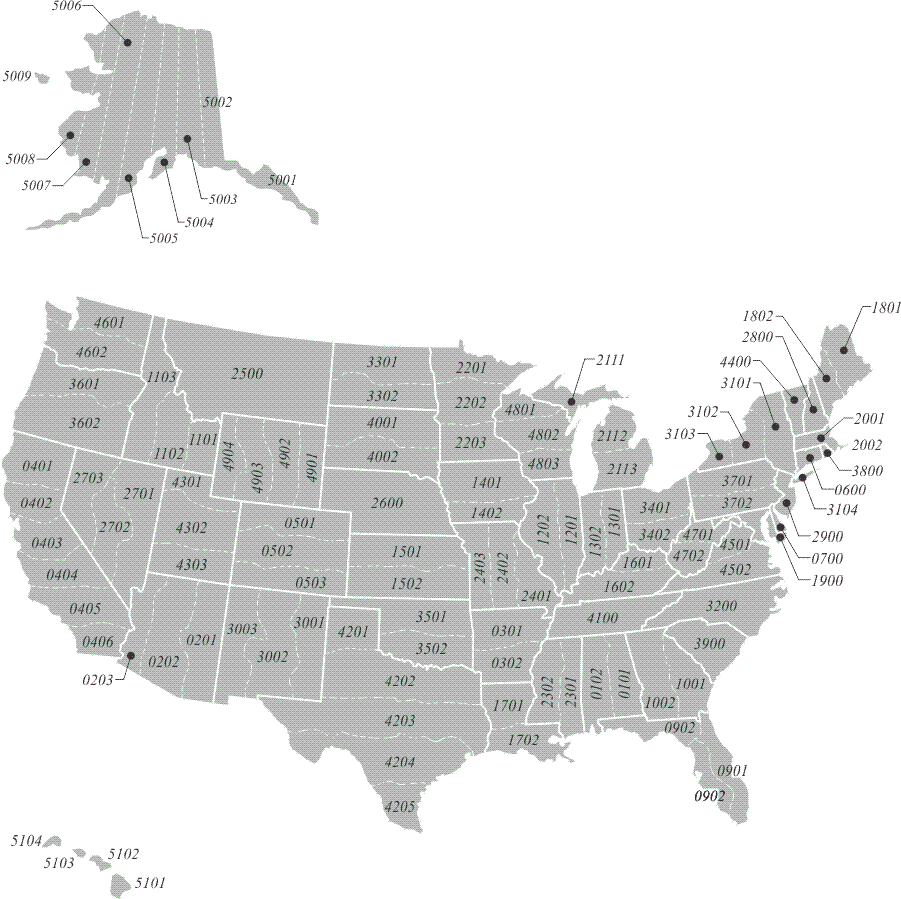
In several instances, the boundaries of State Plane Coordinate Zones today, SPCS83, the State Plane Coordinate System based on NAD83 2011 (2010.0) and its reference ellipsoid GRS80, differ from the original zone boundaries. The foundation of the original State Plane Coordinate System, SPCS27 was NAD27 and its reference ellipsoid Clarke 1866. As mentioned earlier, NAD27 geographical coordinates, latitudes and longitudes, differ significantly from those in NAD83 2011 (2010.0). In fact, conversion from geographic coordinates, latitude and longitude, to grid coordinates, y and x, and back is one of the three fundamental conversions in the State Plane Coordinate system. It is important because the whole objective of the SPCS is to allow the user to work in plane coordinates, but still have the option of expressing any of the points under consideration in either latitude and longitude or State Plane Coordinates without significant loss of accuracy. Therefore, when geodetic control was migrated from NAD27 to NAD83 2011 (2010.0), the State Plane Coordinate System had to go along. When the migration was undertaken in the 1970s, it presented an opportunity for an overhaul of the system. Many options were considered, but in the end, just a few changes were made. One of the reasons for the conservative approach was the fact that 37 states had passed legislation supporting the use of State Plane Coordinates. Nevertheless, some zones got new numbers, and some of the zones changed. The zones are numbered in the SPCS83 system known as FIPS. FIPS stands for Federal Information Processing Standard, and each SPCS83 zone has been given a FIPS number. These days, the zones are often known as FIPS zones. SPCS27 zones did not have these FIPS numbers. As mentioned earlier, the original goal was to keep each zone small enough to ensure that the scale distortion was 1 part in 10,000 or less, but when the SPCS83 was designed, that scale was not maintained in some states. In five states, some SPCS27 zones were eliminated altogether and the areas they had covered were consolidated into one zone or added to adjoining zones. In three of those states, the result was one single large zone. Those states are South Carolina, Montana, and Nebraska. In SPCS27, South Carolina and Nebraska had two zones; in SPCS83, they have just one, FIPS zone 3900 and FIPS zone 2600, respectively. Montana previously had three zones. It has one, FIPS zone 2500. Therefore, because the area covered by these single zones has become so large, they are not limited by the 1 part in 10,000 standard. California eliminated zone 7 and added that area to FIPS zone 0405, formerly zone 5. Two zones previously covered Puerto Rico and the Virgin Islands. They have one. It is FIPS zone 5200. In Michigan, three Transverse Mercator zones were entirely eliminated.
In both the Transverse Mercator and the Lambert Conic projection, the positions of the axes are similar in all SPCS zones. As you can see in the illustration, each zone has a central meridian. These central meridians are true meridians of longitude near the geometric center of the zone. Please note that the central meridian is not the y-axis. If it were the y-axis negative coordinates would result. To avoid them, the actual y-axis is moved far to the west of the zone itself. In the old SPCS27 arrangement, the y-axis was 2,000,000 feet west from the central meridian in the Lambert Conic projection and 500,000 feet in the Transverse Mercator projection. In the SPCS83 design, those constants have been changed. The most common values are 600,000 meters for the Lambert Conic and 200,000 meters for the Transverse Mercator. However, there is a good deal of variation in these numbers from state to state and zone to zone. In all cases, however, the y-axis is still far to the west of the zone and there are no negative State Plane Coordinates. No negative coordinates, because the x-axis, also known as the baseline, is far to the south of the zone. Where the x-axis and y-axis intersect is the origin of the zone, and that is always south and west of the zone itself. This configuration of the axes ensures that all State Plane Coordinates occur in the first quadrant and are, therefore, always positive.
It is important to note that the fundamental unit for SPCS27 was the U.S. survey foot, but "the U.S. survey foot will be phased out as part of the modernization of the National Spatial Reference System (NSRS). From this point forward, the international foot will be simply called the foot." https://www.nist.gov/pml/us-surveyfoot. The fundamental unit for SPCS83, it is the meter.

This brings us to the scale factor, also known as the K factor and the projection factor. It was this factor that the original design of the State Plane Coordinate system sought to limit to 1 part in 10,000. As implied by that effort, scale factors are ratios that can be used as multipliers to convert ellipsoidal lengths, also known as geodetic distances, to lengths on the map projection surface, also known as grid distances, and vice versa. Please notice that the geodetic distance is the distance on the ellipsoid of reference, not the distance measured on the surface of the earth. So, the geodetic length of a line, on the ellipsoid, multiplied by the appropriate scale factor will give you the grid length of that line on the state plane (the map). And the grid length multiplied by the inverse of that same scale factor would bring you back to the geodetic length again. There's another factor that will get you from topographic surface of the earth —where the measurement was made— down to the ellipsoid. However, at the moment we're talking about the scale factor. Here in this image, you see a state plane, and a horizontal line is indicated between the bases of the red arrows. Please notice that between the standard lines, the scale is too small on the state plane. And outside the standard lines, the scale is too large on the state plane. So, the line between the bases of those two red arrows on the ellipsoid of reference will be projected inward from the ellipsoid to the state plane. As it's projected inward —the line shortens. That means that between the intersection of standard lines, the grid (state plane) is under the ellipsoid. In that area, a distance from one point to another is longer on the ellipsoid than on the state plane. This means that right in the middle of the State Plane coordinate systems zone, the scale is at its minimum. In the middle, a typical minimum State Plane coordinate scale factor is not less than 0.9999. Outside of the standard lines, the grid (state plane) is above the ellipsoid where the distance from one point to another is shorter on the ellipsoid than it is on the state plane. There, at the edge of the zone, a maximum typical State Plane coordinate system scale factor is generally not more than 1.0001.
The projection used most on states that are longest from east to west is the Lambert Conic. In this projection, the scale factor for east-west lines is constant. In other words, the scale factor is the same all along the line. One way to think about this is to recall that the distance between the ellipsoid and the map projection surface does not change east to west in that projection. On the other hand, along a north-south line, the scale factor is constantly changing on the Lambert Conic. And it is no surprise then to see that the distance between the ellipsoid and the map projection surface is always changing along the north to south line in that projection. But looking at the Transverse Mercator projection, the projection used most on states longest north to south, the situation is exactly reversed. In that case, the scale factor is the same all along a north-south line, and changes constantly along an east-west line.
Both the Transverse Mercator and the Lambert Conic used a secant projection surface and originally restricted the width to 158 miles. These were two strategies used to limit scale factors when the State Plane Coordinate systems were designed. Where that was not optimum, the width was sometimes made smaller, which means the distortion was lessened. As the belt of the ellipsoid projected onto the map narrows, the distortion gets smaller. For example, Connecticut is less than 80 miles wide north to south. It has only one zone. Along its northern and southern boundaries, outside of the standard parallels, the scale factor is 1 part in 40,000, a fourfold improvement over 1 part in 10,000. And in the middle of the state, the scale factor is 1 part in 79,000, nearly an eightfold increase. On the other hand, the scale factor was allowed to get a little bit smaller than 1 part in 10,000 in Texas. By doing that, the state was covered completely with five zones. And among the guiding principles in 1933 was covering the states with as few zones as possible and having zone boundaries follow county lines. Still it requires ten zones and all three projections to cover Alaska.
When SPCS 27 was current, scale factors were interpolated from tables published for each state. In the tables for states in which the Lambert Conic projection was used, scale factors change north–south with the changes in latitude. In the tables for states in which the Transverse Mercator projection was used, scale factors change east-west with the changes in x-coordinate. Today, scale factors are not interpolated from tables for SPCS83. For both the Transverse Mercator and the Lambert Conic projections, they are calculated directly from equations. There are also several software applications that can be used to automatically calculate scale factors for particular stations. They can be used to convert latitudes and longitudes to State Plane Coordinates. Given the latitude and longitude of the stations under consideration, part of the available output from these programs is typically the scale factors for those stations. To illustrate the use of these factors, consider a line with a length on the ellipsoid of 130,210.44 feet, a bit over 24 miles. That would be its geodetic distance. Suppose that the scale factor for that line was 0.9999536, then the grid distance along the line would be:
Geodetic Distance * Scale Factor = Grid Distance
130,210.44 ft. * 0.999953617 = 130,204.40 ft.
The difference between the longer geodetic distance and the shorter grid distance here is a little more than 6 feet. That is actually better than 1 part in 20,000; please recall that the 1 part in 10,000 ratio was originally considered the maximum. Distortion lessens, and the scale factor approaches 1 as a line nears a standard parallel. Please also recall that on the Lambert projection, an east–west line, that is a line that follows a parallel of latitude, has the same scale factor at both ends and throughout. However, a line that bears in any other direction will have a different scale factor at each end. A north–south line will have a great difference in the scale factor at its north end compared with the scale factor of its south end.
Where K is the scale factor for a line, K1 is the scale factor at one end of the line and K2 is the scale factor at the other end of the line. Scale factor varies with the latitude in the Lambert projection. For example, suppose the point at the north end of the 24-mile line is called Stormy and has a geographic coordinate of:
37º46’00.7225”
103º46’35.3195”
and at the south end the point is known as Seven with a geographic coordinate of:
37º30’43.5867”
104º05’26.5420”

The scale factor for point Seven is 0.99996113 and the scale factor for point Stormy is 0.99994609. It happens that point Seven is further south and closer to the standard parallel than is point Stormy, and it therefore follows that the scale factor at Seven is closer to 1. It would be exactly 1 if it were on the standard parallel, which is why the standard parallels are called lines of exact scale. The typical scale factor for the line is the average of the scale factors at the two end points:
Deriving the scale factor at each end and averaging them is the usual method for calculating the scale factor of a line. The average of the two is sometimes called Km.
However, it can also be done by the precise method K = K1 + K2 + 4Km/6
Elevation Factor

But, that is not the whole story when it comes to reducing distance to the State Plane Coordinate grid. Measurement of lines must always be done on the topographic surface of the Earth, and not on the ellipsoid. Therefore, the first step in deriving a grid distance must be moving a measured line from the Earth to the ellipsoid. The scale factor moves us from the ellipsoid to the state plane (aka grid). However, as mentioned here, the measurements are not made on the ellipsoid. They are made on the surface of the Earth. If we're going to measure the line from one point to another — from station Boulder to station Peak as shown in the illustration— that distance would be measured on the surface of the Earth. To move from the surface of the Earth down to the ellipsoid, we need to have what's known as an elevation factor. Typically, the elevation factor for a line is the average of the elevation factors at each end of the line. For example, the average of the elevation factor at station Boulder (h1), and the elevation factor at station Peak (h2) is the elevation factor for the line (hAvg). That would give the elevation factor for the line Boulder-Peak. Once the elevation factor is available, it is multiplied with the scale factor. The result is known as the combined factor. The combined factor will move the line from the topographic surface of the Earth to the state plane (aka grid).
In the illustration, you may have noticed the approximate radius of the Earth, 20,906,000 feet. It is shown from the center of mass of the Earth up to the ellipsoid. It is an approximation used in creating this elevation factor.
In other words, converting a distance measured on the topographic surface to a geodetic distance on the reference ellipsoid is done with another ratio that is also used as a multiplier. Originally, this factor had a rather unfortunate name. It used to be known as the sea level factor in SPCS27. It was given that name because as you may recall that when NAD27 was established using the Clarke 1866 reference ellipsoid, the distance between the ellipsoid and the geoid was declared to be zero at Meades Ranch in Kansas. That meant that in the middle of the country the sea level surface, the geoid, and the ellipsoid were coincident by definition. And since the Clarke 1866 ellipsoid fit the United States quite well, the separation between the two surfaces, the ellipsoid and geoid, only grew to about 12 meters anywhere in the country. With such a small distance between them, many practitioners at the time took the point of view that, for all practical purposes, the ellipsoid and the geoid were in the same place. And that place was called sea level. Hence, reducing a distance measure on the surface of the Earth to the ellipsoid was said to be reducing it to sea level.
Today, that idea and that name for the factor are misleading because, of course, the GRS80 ellipsoid on which NAD83 is based is certainly not the same as Mean Sea Level. The separation between the geoid and ellipsoid can grow as large as 53 meters. And technology by which lines are measured has improved dramatically. Therefore, in SPCS83, the factor for reducing a measured distance to the ellipsoid is known as the ellipsoid factor. In any case, both the old and the new name can be covered under the name the elevation factor. Regardless of the name applied to the factor, it is a ratio. The ratio is the relationship between an approximation of the Earth’s radius and that same approximation with the mean ellipsoidal height of the measured line added to it. For example, consider station Boulder and station Peak illustrated in the figure above.
Boulder
- N39º59’29.1299”
- W105º15’39.6758”
Peak
- N40º01’19.1582”
- W105º30’55.1283”
The distance between these two stations is 72,126.21 feet. This distance is sometimes called the ground distance, or the horizontal distance at mean elevation. In other words, it is not the slope distance but rather the distance between them corrected to an averaged horizontal plane, as is common practice. For practical purposes, then, this is the distance between the two stations on the topographic surface of the Earth. On the way to finding the grid distance Boulder to Peak, there is the interim step, calculating the geodetic distance between them, that is the distance on the ellipsoid. We need the elevation factor, and here is how it is determined.
The ellipsoidal height of Boulder, h1, is 5,437 feet. The ellipsoidal height of Peak, h2, is 9,099 feet. The approximate radius of the Earth, traditionally used in this work, is 20,906,000 feet. The elevation factor is calculated:
This factor then is the ratio used to move the ground distance down to the ellipsoid, down to the geodetic distance.
It is possible to refine the calculation of the elevation factor by using an average of the actual radial distances from the center of the ellipsoid to the end points of the line, rather than the approximate 20,906,000 feet. In the area of stations Boulder and Peak, the average ellipsoidal radius is actually a bit longer, but it is worth noting that within the continental United States such variation will not cause a calculated geodetic distance to differ significantly.
Grid and Geodetic Azimuths

You will find that every zone in a State Plane coordinate system has a central meridian. In Colorado, the central meridian is 105 degrees, 30 minutes West Longitude, as shown here, on the left you have station D266 and on the right, station Fink. Notice that, in both cases, that grid north is exactly parallel with the central meridian. This is the convention for any plane coordinate system, so that north is always up, and always the same direction. All the norths are parallel in the plane systems; this is, of course, unrealistic. Meridians converge on the surface of the Earth. Therefore, there is a value, shown here in blue, called convergence. Convergence is the difference between geodetic north and grid north. You see over here on the right at station Fink, the convergence is plus 17.2 arcseconds. All the convergence angles east of the Central Meridian are positive. On the left, at station D266, the convergence is minus 40.0 arcseconds. All the convergence angles west of the Central Meridian are negative.
Please note that the sum of the grid azimuths (in red) at station Fink and station D266 is 360 degrees. This is a direct result of the grid north lines being parallel with each other. However, the sum of the geodetic azimuths (in green) at station Fink and station D266 is not 360 degrees. This is a direct result of the geodetic north lines converging. On the Earth they are not parallel with each other. The bottom line is this. On the State Plane coordinate grid, north is always parallel with the central meridian, but at the points on the Earth, north is along the meridian that passes through them. They are certainly not parallel with one another and certainly not parallel with the central meridian.
Universal Transverse Mercator
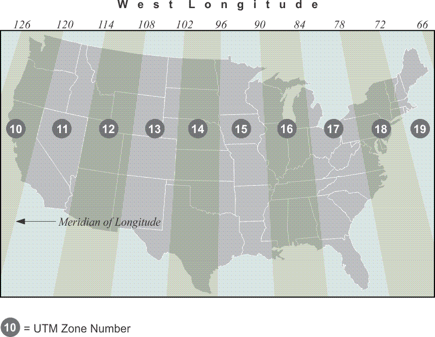
A plane coordinate system that is convenient for GIS work over large areas is the Universal Transverse Mercator (UTM) system. UTM with the Universal Polar Stereographic system covers the world in one consistent system. It is four times less precise than typical State Plane Coordinate systems, with a scale factor that reaches 0.9996. A Universal Transverse Mercator zone embraces a much larger portion of the earth than does a state plane coordinate zone. When you get a larger bite, a larger portion of the earth, the scale factor is less attractive. Yet, the ease of using UTM and its worldwide coverage makes it very attractive for work that would otherwise have to cross many different SPCS zones. For example, nearly all National Geospatial-Intelligence Agency (NGA) topographic maps, U.S. Geological Survey (USGS) quad sheets, and many aeronautical charts show the UTM grid lines. It is often said that UTM is a military system created by the U.S. Army; but several nations, and the North Atlantic Treaty Organization (NATO), played roles in its creation after World War II. At that time, the goal was to design a consistent coordinate system that could promote cooperation between the military organizations of several nations. Before the introduction of UTM, allies found that their differing systems hindered the synchronization of military operations. Conferences were held on the subject from 1945 to 1951, with representatives from Belgium, Portugal, France, and Britain, and the outlines of the present UTM system were developed. By 1951, the U.S. Army introduced a system that was very similar to that currently used. The UTM projection divides the world into 60 zones that begin at longitude 180º, the International Date Line. Zone 1 is from 180° to the 174° W longitude. The conterminous United States is within UTM zones 10 to 19. Here is a convenient way to find the zone number for a particular longitude. Consider west longitude negative and east longitude positive, add 180° and divide by 6. Any answer greater than an integer is rounded to the next highest integer, and you have the zone. For example, Denver, Colorado is near 105° W. Longitude, –105°.
–105° + 180° = 75°
75 °/ 6 = 12.50<
Round up to 13
Therefore, Denver, Colorado, is in UTM Zone 13.
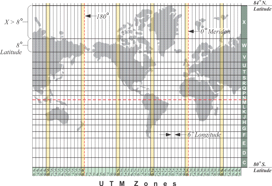
All UTM zones have a width of 6° of longitude. From north to south, the zones extend from 84° N latitude to 80° S latitude. Originally the northern limit was at 80° N latitude and the southern 80° S latitude. On the south, the latitude is a small circle that conveniently traverses the ocean well south of Africa, Australia, and South America. However, 80° N latitude was found to exclude parts of Russia and Greenland and was extended to 84° N latitude. You will notice letters of the alphabet along the right edge of the illustration. There are a few letters missing. You see C,D,E, F, G,H —but there is no I, because it's too close to the number 1 and could be confused— J,K, L, M, N —but there is no O, it could be confused for the number zero— P,Q, R, S,T U, V, W, X, there is no Y, — and finally there is Z. I point this out because there are GPS/GNSS systems that use these letter designations along with the number of the UTM zone to identify a particular quadrangle. For example, C21 would be the square that you see just immediately above 21 in the Southern Hemisphere. This is a useful method of referring to a particular quadrangle in a particular UTM zone. The designations are also used by the military.
Unlike any of the systems previously discussed, every coordinate in a UTM zone occurs twice, once in the Northern Hemisphere and once in the Southern Hemisphere. This is a consequence of the fact that there are two origins in each UTM zone. The origin for the portion of the zone north of the equator is moved 500 km west of the intersection of the zone’s central meridian and the equator. This arrangement ensures that all of the coordinates for that zone in the Northern Hemisphere will be positive. The origin for the coordinates in the Southern Hemisphere for the same zone is 500 km west of the central meridian, as well. But in the Southern Hemisphere, the origin is not on the equator, it is 10,000 km south of it, close to the South Pole. This orientation of the origin guarantees that all of the coordinates in the Southern Hemisphere are in the first quadrant and are positive. In other words, the intersection of each zone’s central meridian with the equator defines its origin of coordinates. In the southern hemisphere, each origin is given the coordinates:
easting = X0 = 500, 000 meters, and northing = Y0 = 10,000,000 meters
In the northern hemisphere, the values are:
easting = X0 = 500, 000 meters, and northing = Y0 = 0 meters, at the origin
The UTM zones nearly cover the earth, except the Polar Regions, which are covered by two azimuthal polar zones called the Universal Polar Stereographic (UPS) projection.

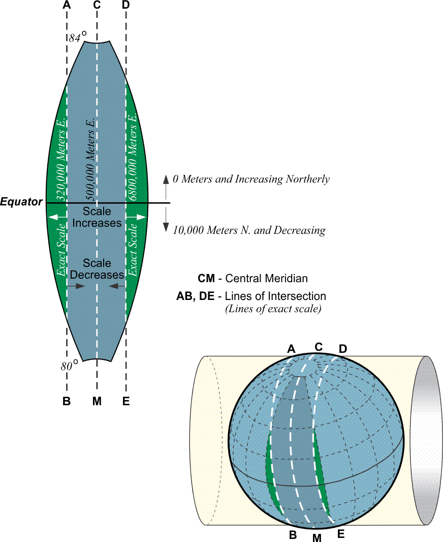
The foundation of the 60 UTM zones is a secant Transverse Mercator projection, very similar to those used in some State Plane Coordinate systems. The central meridian of the zones is exactly in the middle. For example, in Zone 1, from 180° W to the 174° W longitude, the central meridian is 177° W longitude, so each zone extends 3 degrees east and west from its central meridian. The UTM secant projection gives approximately 180 kilometers between the lines of exact scale where the cylinder intersects the ellipsoid. The scale factor grows from 0.9996 along the central meridian of a UTM zone to 1.00000 at 180 km to the east and west. Please recall that SPCS zones are usually more limited in width, ~158 miles, and, therefore, have a smaller range of scale factors than do the UTM zones. In State Plane coordinates, the scale factor is usually no more than 1 part in 10,000. In UTM coordinates, it can be as large as 1 part in 2500. The reference ellipsoids for UTM coordinates vary.
Heights


A point on the earth’s surface is not completely defined by its latitude and longitude. In such a context, there is, of course, a third element, that of height. Surveyors have traditionally referred to this component of a position as its elevation. One classical method of determining elevations is spirit leveling. A level, correctly oriented at a point on the surface of the earth, defines a line parallel to the geoid at that point. Therefore, the elevations determined by level circuits are orthometric; that is, they are defined by their vertical distance above the geoid as it would be measured along a plumb line. However, orthometric elevations are not directly available from the geocentric position vectors derived from GPS/GNSS measurements. In a normal course of things, a coordinate —YX, or northing easting, or latitude and longitude— is not fully a definition of a position. We've discussed also Earth-Centered, Earth-Fixed XYZ coordinates, but it is typical for a horizontal coordinate to be given a height, or elevation. This third element, was most often originally determined by spirit leveling or, in some cases, by a technique known as trigonometric leveling. Despite the surveying method that was used in the past, it was based on optical instruments oriented to gravity, therefore oriented to the geoid. Therefore, the heights were based upon gravity. There is a long legacy of benchmarks, recorded heights, and archives that are based upon this sort of methodology of determining heights. And so, this is what it follows that these values are generally what we think of as elevations —we think of orthometric heights based upon gravity.
Ellipsoidal Heights

As mentioned before, modern geodetic datums rely on the surfaces of geocentric ellipsoids to approximate the surface of the Earth. But the actual surface of the Earth does not coincide with these nice smooth surfaces, even though that is where the points represented by the coordinate pairs lay. Abstract points may be on the ellipsoid, but the physical features those coordinates intend to represent are on the Earth. Though the intention is for the Earth and the ellipsoid to have the same center, the surfaces of the two figures are certainly not in the same place. There is a distance between them. The distance represented by a coordinate pair on the reference ellipsoid to the point on the surface of the Earth can be measured along a line perpendicular to the ellipsoid - which differs from the direction of gravity. This distance is known by more than one name. It is called the ellipsoidal height, and it is also called the geodetic height and is usually symbolized by h. In the illustration, you see an ellipsoidal height of +2,644 meters. The concept is straightforward. A reference ellipsoid may be above or below the surface of the Earth at a particular place. If the ellipsoid’s surface is below the surface of the Earth at the point, the ellipsoidal height has a positive sign; if the ellipsoid’s surface is above the surface of the Earth at the point, the ellipsoidal height has a negative sign.

It is quite impossible to actually set up an instrument on the ellipsoid. That makes it tough to measure ellipsoidal height using surveying instruments. In other words, ellipsoidal height is not what most people think of as an elevation. Said another way, an ellipsoidal height is not measured in the direction of gravity. It is not measured in the conventional sense of down or up. In the illustration, there is an instrument level on the topographic surface of the Earth. The direction of gravity does not coincide with the perpendicular to the ellipsoid.

Nevertheless, the ellipsoidal height of a point is readily determined using a GPS/GNSS receiver. GPS/GNSS can be used to discover the distance from the geocenter of the Earth to any point on the Earth, or above it for that matter. In other words, it has the capability of determining three-dimensional coordinates of a point in a short time. It can provide latitude and longitude, and if the system has the parameters of the reference ellipsoid in its software, it can calculate the ellipsoidal height. The relationship between points can be further expressed in the ECEF coordinates, X, Y, and Z, or in a Local Geodetic Horizon System (LHGS) of north, east, and up. Actually, in a manner of speaking, ellipsoidal heights are new, at least in common usage, since they could not be easily determined until GPS/GNSS became a practical tool in the 1980s.
You may wonder why in the world spend any time at all on this bizarre idea of an ellipsoid height. Since you can't measure it directly, you can't set up on the ellipsoid, what's the point? Well, here's the point. As you see in this image, the ellipsoid height, not the orthometric height, is what is determined directly from a GPS/GNSS measurement. The GPS/GNSS satellites orbit around the center of mass of the Earth. They have no concept of where the surface of the Earth is. Your receiver, which is on the surface of the Earth, of course, could just as well be in outer space as far as the GPS/GNSS coordinate or Earth-Centered-Earth-Fixed XYZ is concerned. Starting from the 3D Cartesian coordinate and given a particular ellipsoid on which to work, it is possible for the computer in your GPS/GNSS receiver to calculate a latitude and longitude. It will base that latitude and longitude on the ellipsoidal parameters in its microcomputer. It follows that the height that is determined up to the station that you're interested in will also be based upon the ellipsoid.

However, ellipsoidal heights are not all the same, because reference ellipsoids, or sometimes just their origins, can differ. For example, an ellipsoidal height expressed in ITRF might be based on an ellipsoid with exactly the same shape as the NAD83 ellipsoid, GRS80. Nevertheless, the heights would be different because the origin has a different relationship with the Earth’s surface. It's worthwhile to note that ellipsoidal heights vary as the ellipsoid changes. As the reference frame (datum) changes, the ellipsoid height changes. And that's what this image here is intended to represent. There is an approximately 2.24 meter separation between the origin of NAD83, the GRS80 ellipsoid, the ITRF ellipsoid. Therefore, the heights —the small h, the ellipsoid height— derived from each of these would be different.
The Geoid

Any object in the earth’s gravitational field has potential energy derived from being pulled toward the Earth. Quantifying this potential energy is one way to talk about height, because the amount of potential energy an object derives from the force of gravity is related to its height. There are an infinite number of points where the potential of gravity is always the same. They are known as equipotential surfaces. Mean Sea Level itself is not an equipotential surface at all, of course. Forces other than gravity affect it, forces such as temperature, salinity, currents, wind, and so forth. The geoid, on the other hand, is defined by gravity alone. The geoid is the particular equipotential surface arranged to fit Mean Sea Level as well as possible, in at least squares sense. The geoid and the ellipsoid are not the same. Remember that the legacy heights determined by optical instruments in the past were always relative to the geoid, because, of course, the instruments were oriented to gravity. However, GPS/GNSS heights are related directly at least to the ellipsoid —two different surfaces.

So, while there is a relationship between Mean Sea Level and the geoid, they are not the same. They could be the same if the oceans of the world could be utterly still, completely free of currents, tides, friction, variations in temperature, and all other physical forces, except gravity. However, these unavoidable forces actually cause Mean Sea Level to deviate up to 1, even 2, meters from the geoid.

The geoid is completely is not smooth and continuous. It is lumpy, because gravity is not consistent across the surface of the earth. At every point, gravity has a magnitude and a direction, but these vectors do not all have the same direction or magnitude. Some parts of the earth are denser than others. Where the earth is denser, there is more gravity, and the fact that the earth is not a sphere also affects gravity. The geoid undulates with the uneven distribution of the mass of the earth and has all the irregularity that the attendant variation in gravity implies. In fact, the separation between the lumpy surface of the geoid and the smooth GRS80 ellipsoid worldwide varies from about +85 meters west of Ireland to about -106 meters, the latter in the area south of India near Ceylon.

In the conterminous United States, sometimes-abbreviated CONUS, the distances between the geoid and the GRS80 ellipsoid, known as geoid heights, are less. They vary from about –8 meters to about –53 meters.
Height Conversion


A geoidal height is the distance measured along a line perpendicular to the ellipsoid of reference to the geoid. Also, as you can see in the illustration, these geoid heights are negative. They are usually symbolized, N. If the geoid is above the ellipsoid, N is positive; if the geoid is below the ellipsoid, N is negative. It is negative here because the geoid is underneath the ellipsoid throughout the conterminous United States. In Alaska, it is the other way around; the ellipsoid is underneath the geoid and N is positive.
Please recall that an ellipsoid height is symbolized, h. The ellipsoid height is also measured along a line perpendicular to the ellipsoid of reference, but to a point on the surface of the Earth.
However, an orthometric height, symbolized, H, is measured along a plumb line from the geoid to a point on the surface of the Earth. By using the formula,
H = h – N
one can convert an ellipsoidal height, h, derived say from a GPS/GNSS observation, into an orthometric height, H, by knowing the extent of geoid-ellipsoid separation, also known as the geoidal height, N, at that point. The ellipsoid height of a particular point is actually smaller than the orthometric height throughout the conterminous United States.
The formula H = h – N does not account for the fact that the plumb line along which an orthometric height is measured is curved, as you see in the figure above. Curved, because it is perpendicular with each and every equipotential surface through which it passes. The equipotential surfaces are not parallel with each other. They converge toward the pole because the Earth is oblate therefore, the plumb line must curve to maintain perpendicularity with them all. This deviation of a plumb line from the perpendicular to the ellipsoid reaches about 1 minute of arc in only the most extreme cases. Therefore, any height difference that is caused by the curvature is negligible. It would take a height of over 6 miles for the curvature to amount to even 1 mm of difference in height.
Geoidal Models

Major improvements have been made over the past quarter-century or so in mapping the geoid on both national and global scales. And because there are large complex variations in the geoid related to both the density and relief of the earth, geoid models and interpolation software have been developed to support the conversion of GPS elevations to orthometric elevations. For example, in early 1991, NGS presented a program known as GEOID90. This program allowed a user to find N, the geoidal height, in meters for any NAD83 latitude and longitude in the United States.
The GEOID90 model was computed at the end of 1990, using over a million gravity observations. It was followed by the GEOID93 model. It was computed at the beginning of 1993, using more than 5 times the number of gravity values used to create GEOID90. Both provided a grid of geoid height values in 3 minutes of latitude by 3 minutes of longitude grid with an accuracy of about 10 cm. Next, the GEOID96 model resulted in a gravimetric geoid height grid in a 2 minutes of latitude by 2 minutes of longitude grid.
GEOID99 covered the conterminous United States, and it includes U.S. Virgin Islands, Puerto Rico, Hawaii, and Alaska. The grid is 1 degree of latitude by 1 degree of longitude, and it is the first to combine gravity values with GPS ellipsoid heights on previously leveled benchmarks. According to NGS, “When comparing the GEOID99 model with GPS ellipsoid heights in the NAD 83 reference frame and leveling in the NAVD 88 datum, it is seen that GEOID99 has roughly a 4.6 cm absolute accuracy (one sigma) in the region of GPS on benchmark coverage. GEOID03 superseded the previous models for the continental United States. It was followed by GEOID09, and the current geoid model in place is known as GEOID18.
NGS has an ongoing project known gravity mapping project known as GRAV-D, "The gravity-based vertical datum resulting from this project will be accurate at the 2 cm level where possible for much of the country. The proposal is official policy for NGS and is included in the NGS 10 year plan. The project is currently underway and actively collecting gravity data across the United States and its holdings." https://geodesy.noaa.gov/GRAV-D/
Discussion
Discussion Instructions
To continue the discussion begun by this lesson, I would like to pose this question:
If you were building a GIS at an intercontinental scale, what coordinate system would you use? Why? If you were building a GIS at a continental scale, what coordinate system would you use? Why? If you were building a GIS at a county scale, what coordinate system would you use? Why? And how would you store GPS derived heights in your database?
To participate in the discussion, please go to the Lesson 6 Discussion Forum in Canvas. (That forum can be accessed at any time by going to the GEOG 862 course in Canvas and then looking inside the Lesson 6 module.)
Summary
Despite the fact that the assumption of a flat earth is fundamentally wrong, calculation of areas, angles, and lengths using latitude and longitude can be complicated, so plane coordinates persist. Therefore, the projection of points from the Earth’s surface onto a reference ellipsoid and finally onto flat maps is still viable.
Heights, orthometric, ellipsoidal and dynamic, may appear, at first, to be simple. However, understanding them in a world of satellite positioning requires knowledge of the surfaces to which they refer and the methods by which they are derived. Perhaps this lesson has provided some of that understanding.
Next, we will delve a little deeper into the details of the most commonly used GPS techniques; Static, DGPS and RTK. At this point, we are really beginning to get into some of the most immediately applicable aspects of new developments in the field.
Before you go on to Lesson 7, double-check the Lesson 6 Checklist to make sure you have completed all of the activities listed there.
Lesson 7: Static Global Positioning System Surveying
The links below provide an outline of the material for this lesson. Be sure to carefully read through the entire lesson before returning to Canvas to submit your assignments.
Lesson 7 Overview
Overview
Static GPS/GNSS, where the receiver is stationary, is the original GPS/GNSS method. It is still the preferred approach for establishing the most accurate positions, the control. In many ways. For example, some processing and data checking should be performed on a daily basis during a GPS/GNSS project. Blunders from operators, noisy data, and unhealthy satellites can corrupt entire sessions. In any case, left undetected, such dissolution can jeopardize an entire project. These weaknesses in the data can sometimes be prevented before they happen by best practices such as optimization of the observation schedule. GPS/GNSS measurements are still composed of fundamentally biased ranges. Therefore, the goal remains to mitigate the biases and extract the true ranges. In this lesson, we start to get into the real details of how static GPS/GNSS work is done.
Objectives
At the successful completion of this lesson, students should be able to:
- discuss the difference between precision and accuracy
- discuss the basics of planning a static GPS/GNSS survey;
- recognize the role of NGS control;
- explain Continuously Operating Reference Stations;
- explain Static GPS/GNSS project design;
- demonstrate drawing GPS/GNSS baselines
- describe the difference between dependent and independent baselines;
- describe how to calculate the number of sessions necessary for a static survey;
- discuss some of the components of Static GPS/GNSS control such as equipment, station data sheets, visibility diagrams, monumentation and logistics
Questions?
If you have any questions now or at any point during this week, please feel free to post them to the Lesson 7 Discussion Forum. (To access the forum, return to Canvas and navigate to the Lesson 7 Discussion Forum in the Lesson 7 module.) While you are there, feel free to post your own responses if you, too, are able to help out a classmate.
Checklist
Lesson 7 is one week in length. (See the Calendar in Canvas for specific due dates.) To finish this lesson, you must complete the activities listed below. You may find it useful to print this page out first so that you can follow along with the directions.
| Step | Activity | Access/Directions |
|---|---|---|
| 1 | Read the lesson Overview and Checklist. | You are in the Lesson 7 online content now. The Overview page is previous to this page, and you are on the Checklist page right now. |
| 2 | Read Chapter 6 in GPS for Land Surveyors. | Text |
| 3 | Read the lecture material for this lesson. | You are currently on the Checklist page. Click on the links at the bottom of the page to continue to the next page, to return to the previous page, or to go to the top of the lesson. You can also navigate the lecture material via the links in the Lessons menu. |
| 4 | Participate in the Discussion. | To participate in the discussion, please go to the Lesson 7 Discussion Forum in Canvas. (That forum can be accessed at any time by going to the GEOG 862 course in Canvas and then looking inside the Lesson 7 module.) |
| 5 | Write a 2,400 word paper on one topic covered in the course over the previous weeks. | Please submit your paper to the Lesson 7 Paper Drop Box located in the Lesson 7 module. View Calendar in Canvas for specific due date. |
| 6 | Read lesson Summary. | You are in the Lesson 7 online content now. Click on the "Next Page" link to access the Summary. |
Static GPS Control Surveying

Static GPS/GNSS surveying has been used on control surveys from local to statewide to continental extent, and will probably continue to be the preferred technique in those categories. In static GPS/GNSS surveying, the receivers is motionless for a time, usually a relatively long occupation. If a static GPS/GNSS control survey is carefully planned, it usually progresses smoothly. The technology has virtually conquered two stumbling blocks that have defeated the plans of conventional surveyors for generations. Inclement weather does not disrupt GPS/GNSS observations, and a lack of intervisibility between stations is of no concern whatsoever, at least in postprocessed GPS/GNSS. Still, GPS/GNSS is far from so independent of conditions in the sky and on the ground that the process of designing a survey can now be reduced to points-per-day formulas, as some would like. Even with falling costs, the initial investment in GPS/GNSS remains large by most surveyors’ standards. However, there is seldom anything more expensive in a GPS/GNSS project than a surprise.
Planning a Static GPS/GNSS Control Survey: Accuracy and Precision

A Few Words about Accuracy
When planning a GPS/GNSS survey, one of the most important parameters is the accuracy specification. A clear accuracy goal avoids ambiguity both during and after the work is done. First, it is important to remember that there is a difference between precision and accuracy. One aspect of precision can be visualized as the tightness of the clustering of measurements; the closer the grouping, the more precise the measurement. Accuracy, on the other hand, requires one more element. It has to have a truth set. For example, the truth in illustration for A, B and C is the center of the target - without that accuracy is indefinable. In other words, accuracy is not determined by measurement alone. There must also be a standard value or values involved is through the comparison of the measurements with such standard values that the outcome of the work can be found to be sufficiently near the ideal or true value, or not.

For example, on the left in the illustration it may seem at first that the average of the measurements in the GPS-A group are more accurate than the average of those in GPS-B because the GPS-A group is more precise. However, when the true position is introduced on the right it is revealed that the GPS-B group’s average is the more accurate of the two, because accuracy and precision are not the same. When it comes to accuracy, there are other important details too. Local accuracy and network accuracy are not the same. As mentioned earlier, local accuracy, also known as relative accuracy, represents the uncertainty in the positions relative to the other adjacent points to which they are directly connected. Network accuracy, also known as absolute accuracy, requires that a position’s accuracy be specified with respect to an appropriate truth set such as a national geodetic datum. Differentially corrected GPS/GNSS survey procedures which are tied to CORS stations, which represent the National Spatial Reference System of the United States, provide information from which network accuracy can be derived. However, autonomous GPS/GNSS positioning, that is a single receiver without augmentation is not operating relative to any control, local or national. In that context, it is more appropriate to discuss the precision of the results than it is to discuss accuracy.

It is typical for uncertainty in horizontal accuracies to be expressed in a number that is radial. The uncertainties in vertical accuracies are given similarly, but they are linear, not radial. In both cases, the limits are always plus or minus (±). In other words, the reporting standard in the horizontal component is the radius of a circle of uncertainty, such that the true location of the point falls within that circle at some level of reliability, i.e. 95-percent of the time. Also, the reporting standard in the vertical component is a linear uncertainty value, such that the true location of the point falls within ± of that linear uncertainty to some degree of reliability. GPS positioning it is reasonable to expect that the vertical accuracy will be about 1/3 that of horizontal accuracy. If the absolute horizontal accuracy of a GPS position is ±1m then the estimate of the absolute vertical accuracy of the same GPS position would be ~±3m.

Here is a bit more on horizontal accuracy. The illustration shows a spread of positions around a center of the range. As the radius of the error circle grows larger, the certainty that the center of the range is the true position increases (it never reaches 100%).
It is not correct to say that every job suddenly requires the highest achievable accuracy, nor is it correct to say that every GPS/GNSS survey now demands an elaborate design. In some situations, a crew of two, or even one surveyor on-site may carry a GPS/GNSS survey from start to finish with no more planning than minute-to-minute decisions can provide, even though the basis and the content of those decisions may be quite different from those made in a conventional survey.

In areas that are not heavily treed and generally free of overhead obstructions, sufficient accuracy may be possible without a prior design of any significance. But while it is certainly unlikely that a survey of photocontrol or work on a cleared construction site would present overhead obstructions problems comparable with a static GPS/GNSS control survey in the Rocky Mountains, even such open work may demand preliminary attention. For example, just the location of appropriate vertical and horizontal control stations or obtaining permits for access across privately owned property or government installations can be critical to the success of the work. An initial visit to the site of the survey is not always possible. Today, online mapping browsers are making virtual site evaluation possible as well. Topography as it affects the line of sight between stations is of no concern on a static GPS/GNSS project, but its influence on transportation from station to station is a primary consideration. Perhaps some areas are only accessible by helicopter or other special vehicle. Initial inquiries can be made. Roads may be excellent in one area of the project and poor in another. The general density of vegetation, buildings, or fences may open general questions of overhead obstruction or multipath. The pattern of land ownership relative to the location of project points may raise or lower the level of concern about obtaining permission to cross property. It is now relatively easy to do GPS/GNSS surveying, that is, when everything works the way it's supposed to. However, if there are going to be troubles like access to the points, overhead obstructions, work in trees, or helicopter transport, planning needs to be part of the process.
NGS Control Data Sheets


One of the things that is very useful is understanding the existing control that is currently available. Brass tablets and brass caps have been set around the United States by the National Geodetic Survey also known as passive marks. You can retrieve sheets that are similar to what you see in the illustration. These sheets have a great deal of excellent information concerning the coordinates, the quality, and many of the details about existing control points that can be used as checkpoints in any GPS/GNSS survey. Monuments that are the physical manifestation of the National Spatial Reference System (NSRS) and can be occupied with survey equipment are known as passive marks. They can provide reliable control when properly utilized. That utilization should be informed by an understanding of the datasheet that accompanies each station and is easily available online. There is a good deal of information about the passive survey monuments on each individual sheet. In addition to the latitude and longitude, the published data include the state plane coordinates in the appropriate zones. The first line of each data sheet includes the retrieval date. Then the station’s category is indicated. There are several, and among them are Continuously Operating Reference Station, Federal Base Network Control Station, and Cooperative Base Network Control Station. This is followed by the station’s designation, which is its name, and its Point Identification, PID. Either of these may be used to search for the station in the NGS database. The PID is also found all along the left side of each data sheet record and is always two upper case letters followed by four numbers. The state, county, country and U.S. Geological Survey (USGS)-7.5 minute quad name follows. Even though the station is located in the area covered by the quad sheet, it may not actually appear in the map. Under the heading, “Current Survey Control,” you will find the latitude and longitude of the station in NAD83 which is fixed to the North American plate, currently in NAD83 (2011), and its height in NAVD88. The orthometric height in meters is listed as “ORTHO HEIGHT” and followed by the same in feet. When the height is derived from GPS/GNSS observation, a geoid model must be used to determine the orthometric height. The model used is given. Adjustments to NAD27 and NGVD29 datums are a thing of the past. However, these old values may be shown under Superseded Survey Control. Horizontal values may be either Scaled, if the station is a benchmark or Adjusted, if the station is indeed a horizontal control point.
When a date is shown in parentheses after NAD83 in the data sheet, it means that the position has been readjusted. There are 13 sources of vertical control values shown on NGS data sheets. Here are a few of the categories. There is Adjusted, which are given to 3 decimal places and are derived from least squares adjustment of precise leveling. Another category is Posted, which indicates that the station was adjusted after the general NAVD adjustment in 1991. When a station’s elevation has been found by precise leveling but non-rigorous adjustment, it is called Computed. Stations’ vertical values are given to 1 decimal place if they are from GPS/GNSS observation (Obs) or vertical angle measurements (Vert Ang). And they have no decimal places if they were scaled from topographic map, Scaled, or found by conversion from NGVD29 values using the program known as VERTCON. The NGS Data Sheet.
When they are available, earth-centered earth-fixed (ECEF) coordinates are shown in X,Y and Z. These are right-handed system, 3-D Cartesian coordinates and are computed from the position and the ellipsoidal height. They are the same type of X, Y, and Z coordinates presented earlier. These values are followed by the quantity which, when added to an astronomic azimuth, yields a geodetic azimuth, is known as the Laplace correction. It is important to note that NGS uses a clockwise rotation regarding the Laplace correction. The ellipsoid height per the NAD83 ellipsoid is shown followed by the geoid height where the position is covered by NGS’s GEOID program. Photographs of the station may also be available in some cases. When the data sheet is retrieved online, one can use the link provided to bring them up. Also, the geoidal model used is noted. Of course, the first retrieval date at the top of the sheet is valuable to know when the point was last recovered. There's much detail here. I leave it to you to read. But suffice it to say for the objective here, the NGS data sheet is helpful to learn what control is available in a particular area.
Coordinates
NGS data sheets also provide State Plane and Universal Transverse Mercator (UTM) coordinates, the latter only for horizontal control stations. State Plane Coordinates are given in both U.S. Survey Feet or International Feet, and UTM coordinates are given in meters. Azimuths to the primary azimuth mark are clockwise from north and scale factors for conversion from ellipsoidal distances to grid distances. This information may be followed by distances to reference objects. Coordinates are not given for azimuth marks or reference objects on the data sheet.
The Station Mark
Along with mark setting information, the type of monument and the history of mark recovery, the NGS data sheets provide a valuable to-reach description. It begins with the general location of the station. Then starting at a well-known location, the route is described with right and left turns, directions, road names, and the distance traveled along each leg in kilometers. When the mark is reached, the monument is described, and horizontal and vertical ties are shown. Finally, there may be notes about obstructions to GPS/GNSS visibility, and so forth.
Significance of the Information
The value of the description of the monument’s location and the route used to reach it is directly proportional to the date it was prepared and the remoteness of its location. The conditions around older stations often change dramatically when the area has become accessible to the public. If the age and location of a station increases the probability that it has been disturbed or destroyed, then reference monuments can be noted as alternatives worthy of on-site investigation. However, special care ought to be taken to ensure that the reference monuments are not confused with the station marks themselves.
The role of passive marks is undergoing a change as a new North American reference frame takes shape (North American Terrestrial Reference Frame: NATRF). NGS is no longer setting nor maintaining passive marks.
Control from Continuously Operating Networks

The requirement to occupy physical geodetic monuments in the field can be obviated by downloading the tracking data available online from appropriate continuously operating reference stations (CORS) where their density is sufficient. These stations, also known as Active Stations, comprise fiducial networks that support a variety of GPS/GNSS applications. While they are frequently administered by governmental organizations, some are managed by public-private organizations and some are commercial ventures. The most straightforward benefit of CORS is the user’s ability to do relative positioning without operating his own base station, by depending on that role being fulfilled by the network’s reference stations. While CORS can be configured to support differential GPS (DGPS) and real-time kinematic (RTK) applications, as in Real-Time Networks, most networks constantly collect GPS/GNSS tracking data from known positions and archive the observations for subsequent download by users from the Internet.
These days it is quite possible to not have to occupy an existing brass tablet, brass cap, such as indicated on this NGS data sheet. The reason for this is because of the continuously operating reference stations that have been established by the National Geodetic Survey are very useful. These active stations are a network and the most straightforward benefit is that a user can do relative positioning without operating his own base station and by depending on the CORS station, which as you see in this illustration downloads its reference information from tracking the GPS/GNSS network to an archived base station that is available on the Internet. You can access this and then combine it with the GPS/GNSS data that you have collected and post process for a differential, position a relative position, without having to occupy an existing control point on the ground.


In many instances the original impetus of a network of CORS was geodynamic monitoring as illustrated by the GEONET established by the Geographical Survey Institute, GSI, in Japan after the Kobe earthquake. Networks that support the monitoring of the International Terrestrial Reference System, ITRS have been created around the world by the International GNSS Service, IGS, which is a service of the International Association of Geodesy and the Federation of Astronomical and Geophysical Data Analysis Services originally established in 1993. The United States is by no means the only place in which such networks exist.

Here is an illustration of the Southern California Integrated GPS/GNSS Network, SCIGN is a network run by a government-university partnership. More and more of these networks are appearing across the United States, sometimes on a statewide basis, county basis, and other regional designations. These continuously operating stations occupy a known position and then track the full constellation of GPS/GNSS satellites continuously. Then this data is made available, sometimes with a subscription cost, but in the case of NGS for free, and it is available then to do differential positioning of static GPS/GNSS sessions.
More on Continuously Operating Reference Station Networks

NGS Continuously Operating Reference Stations
The NGS CORS network is illustrated here. It includes hundreds of stations constantly logging GPS/GNSS data. The establishment of a CORS network, the result, has been a boon for high-accuracy GPS/GNSS positioning. Surveyors in the United States can take advantage of the CORS network administered by the National Geodetic Survey, NGS. The continental NGS system has two components, the Cooperative CORS and the National CORS. NGS manages the national CORS to support this post-processing for both code and carrier phase observations. The Cooperative CORS system supplements the National CORS system. The NGS does not directly provide the data from the cooperative system of stations. Its stations are managed by participating university, public, and private organizations that operate the sites. These cooperative arrangements mean that we all can use the data free on charge in most cases. That data can then be conveniently downloaded in its original form from the Internet free of charge for up to 30 days after its collection. It is also available later, but after it has been decimated to a 30-second format. The data is available in the Receiver Independent Exchange Format, or RINEX format. The RINEX format allows you to use any type of a receiver to log your data because this RINEX format is available from virtually every kind of standard GPS/GNSS receiver.
Nearly all coordinates provided by NGS for the CORS sites are available in NAD83 (2011) epoch 2010.0. The coordinates of CORS stations are also published in ITRF2014 (2010.0). These positions differ from NAD83(2011). All the coordinates are accompanied by velocities since the stations are moving. These velocities can be used to calculate the stations position at a different date using NGS’s Horizontal Time Dependent Positioning (HTDP) utility.

Here (above) is an illustration of the Horizontal Time-Dependent Positioning website.

At a CORS site, NGS provides the coordinates of the L1 phase center and the Antenna Reference Point (ARP). Generally speaking, it is best to adopt the position that can be physically measured, that means the coordinates given for the ARP. It is the coordinate of the part of the antenna from which the phase center offsets are calculated that is usually the bottom mount. The phase centers of antennas are not immovable points. They actually change slightly, mostly as the elevation of the satellite’s signals change. In any case, the phase centers for L1, L2 and L5 differ from the position of the ARP both vertically and horizontally. NGS provides the position of the phase center on average at a particular CORS site. As most postprocessing software will, given the ARP, provide the correction for the phase center of an antenna, based on antenna type, the ARP is the most convenient coordinate value to use. The distance to the ARP is often given from the bottom of the mount, as indicated by this diagram.
International GNSS Service (IGS)
Like NGS, IGS also provides CORS data. However, it has a global scope. The information on the individual stations can be accessed, including the ITRF Cartesian coordinates and velocities for the IGS sites, but not all the sites are available from IGS servers. The Scripps Orbit and Permanent Array Center (SOPAC) is a convenient access point for IGS data. A virtual map of the available GPS/GNSS networks can be found there.
Tracking data is from international networks. Here you see a graphic of its extent. It's virtually worldwide. You can download the tracking information from these antennas, these known positions, to post-process the data from a roving GPS/GNSS antenna internationally.
The Scripps Orbit and Permanent Array Center

SOPAC is a convenient access point for IGS data.
Static Survey Project Design

Image ID: 1618, NOAA's Historic Coast & Geodetic Survey (C&GS) Collection
Location: Ozark Mountains, Missouri
Photo Date: 1935
Source: http://www.photolib.noaa.gov/cgs/triangulation.html
Publication of the US Dept. of Commerce, NOAA, NOAA Central Library, COAA Privacy Policy / NOAA Desclaimer
Last Updated: April 23, 2007
Static Survey Project Design
The selection of satellites to track, start and stop times, mask elevation angle, assignment of data file names, reference position, bandwidth, and sampling rate are some options useful in the static mode, as other GPS/GNSS surveying methods. These features may appear to be prosaic, but their practicality is not always obvious. For example, satellite selection can seem unnecessary when using a receiver with sufficient independent channels to track all satellites above the receiver’s horizon without difficulty. However, a good survey project design pays dividends by limiting lost time and maximizing productivity. When geodetic surveying was more dependent on optics than electronic signals from space, horizontal control stations were set with station intervisibility in mind, not ease of access. Therefore, it is not surprising that stations established in that way are frequently difficult to reach. Not only are they found on the tops of buildings and mountains, they are also in woods, beside transmission towers, near fences, and generally obstructed from GPS/GNSS signals. The geodetic surveyors that established them could hardly have foreseen a time when a clear view of the sky above their heads would be crucial to high-quality control. The illustration shows some surveyors on a Bilby tower, high above the Ozark Mountains in Missouri. Their observations were done at night with angles turned to far away lights to establish horizontal control by triangulation. It's hardly surprising that at the time surveyors were working on these towers they weren't terribly concerned with the sky visibility at the stations they occupied and set. They were concerned with getting high enough over obstructions to see the other stations.
In fact, it is only recently that most private surveyors have had any routine use for NGS stations. Many station marks have not been occupied for quite a long time. Since the primary monuments are often found deteriorated, overgrown, unstable, or destroyed. The role of passive marks is changing rapidly. In any case, it is a good idea to propose reconnaissance of several more than the absolute minimum of three horizontal control stations. Fewer than three makes any check of their positions virtually impossible. Many more are usually required in a GPS/GNSS route survey. In general, in GPS/GNSS networks, the more -chosen horizontal control stations that are available, the better. Some stations will almost certainly prove unsuitable unless they have been used previously in GPS/GNSS work. The location of the stations, relative to the GPS/GNSS project itself, is also an important consideration in choosing horizontal control. For work other than route surveys, a handy rule of thumb is to divide the project into four quadrants and to choose at least one horizontal control station in each. The actual survey should have at least one horizontal control station in three of the four quadrants. Each of them ought to be as near as possible to the project boundary. Supplementary control in the interior of the network can then be used to add more stability to the network. At a minimum, route surveys require horizontal control at the beginning, the end, and the middle. Long routes should be bridged with control on both sides of the line at appropriate intervals. The standard symbol for indicating horizontal control on the project map is a triangle.
Vertical Control
Those stations with a published accuracy high enough for consideration as vertical control are symbolized by an open square or circle on the map. Those stations that are sufficient for horizontal control are symbolized as triangles. Where there is horizontal and vertical control the symbol is a combination of the triangle and square.

A minimum of four vertical control stations are needed to anchor a GPS/GNSS static network. A large project should have more. In general, the more benchmarks available the better. Vertical control is best located at the four corners of a project. Orthometric elevations are best transferred by means of classic spirit leveling; such work should be built into the project plan when it is necessary. When spirit levels are planned to provide vertical control positions, special care may be necessary to ensure that the precision of such conventional work is as consistent as possible with the rest of the survey. Route surveys require vertical control at the beginning and the end. They should be bridged with benchmarks on both sides of the line at intervals from 5 to 10 km. When the distances involved are too long for spirit leveling to be used effectively, two independent GPS/GNSS measurements may suffice to connect a benchmark to the project. However, it is important to recall the difference between the ellipsoidal heights available from a GPS/GNSS observation and the orthometric elevations yielded by a level circuit.
Plotting Project Points
A solid dot is the standard symbol used to indicate the position of project points. Some variation is used when a distinction must be drawn between those points that are in place and those that must be set.

When its location is appropriate, it is always a good idea to have a vertical or horizontal control station serve double duty as a project point. While the precision of their plotting may vary, it is important that project points be located as precisely as possible even at this preliminary stage. The subsequent observation schedule will depend to some degree on the arrangement of the baselines. Also, the preliminary evaluation of access, obstructions, and other information depends on the position of the project point relative to these features. In the design, the project points are indicated. These are the points on which coordinates are going to be required based upon the control available around them.

Evaluating Access
When all potential control and project positions have been plotted and given a unique identifier, some aspects of the survey can be addressed a bit more specifically. If good roads are favorably located, if open areas are indicated around the stations, and if no station falls in an area where special permission will be required for its occupation, then the preliminary plan of the survey ought to be remarkably trouble-free. However, it is likely that one or more of these conditions will not be so fortunately arranged. The speed and efficiency of transportation from station to station can be assessed to some degree from the project map. It is also wise to remember that while inclement weather does not disturb GPS/GNSS observations whatsoever, without sufficient preparation it can play havoc with surveyors’ ability to reach points over difficult roads or by aircraft. Since in a static GPS/GNSS survey, the control points and the points to be coordinated—the project points—need to be occupied simultaneously, they need to observe the same constellation of satellites at the same time. It's important to be able to be on the station ready to observe when the sessions begin, simultaneously on control and project points.

Planning Offsets
If control stations or project points are located in areas where the map indicates that topography or vegetation will obstruct the satellite’s signals, alternatives may be considered. A shift of the position of a project point into a clear area may be possible where the change does not have a significant effect on the overall network. A control station may also be the basis for a less obstructed position, transferred with a short level circuit or traverse. Of course, such a transfer requires availability of conventional surveying equipment on the project. In situations where such movement is not possible, careful consideration of the actual paths of the satellites at the station itself during on-site reconnaissance may reveal enough windows in the gaps between obstructions to collect sufficient data by strictly defining the observation sessions.
Planning Azimuth Marks
Azimuth marks are a common requirement in GPS/GNSS projects. They are an accompaniment to static GPS/GNSS stations when a client intends to use them to control subsequent conventional surveying work. Of course, the line between the station and the azimuth mark should be as long as convenience and the preservation of line-of-sight allows. It is wise to take care that short baselines do not degrade the overall integrity of the project. Occupations of the station and its azimuth mark should be simultaneous for a direct measurement of the baseline between them. Both should also be tied to the larger network as independent stations. There should be two or more occupations of each station when the distance between them is less than 2 km. An alternative approach may be to derive the azimuth between a GPS/GNSS station and its azimuth mark with an astronomic observation.

Obtaining Permissions
Another aspect of access can be considered when the project map finally shows all the pertinent points. Nothing can bring a well-planned survey to a halt faster than a locked gate, an irate landowner, or a government official that is convinced he should have been consulted previously. To the extent that it is possible from the available mapping, affected private landowners and government jurisdictions should be identified and contacted. Taking this precaution at the earliest stage of the survey planning can increase the chance that the sometimes long process of obtaining permissions, gate keys, badges, or other credentials has a better chance of completion before the survey begins.
Any aspect of a GPS/GNSS survey plan derived from examining mapping, virtual or hardcopy, must be considered preliminarily. Most features change with time, and even those that are relatively constant cannot be portrayed on a map with complete exactitude. Nevertheless, steps toward a coherent workable design can be taken using the information they provide.
Control Project Design Facts

Though much of the preliminary work in producing the plan of a GPS/GNSS survey is a matter of estimation, some hard facts must be considered, too. For example, the number of GPS/GNSS receivers available for the work and the number of satellites above the observer’s horizon at a given time in a given place are two ingredients that can be determined with some certainty. Most GPS/GNSS software packages provide users with routines that help them determine the satellite windows, the periods of time when the largest numbers of satellites are simultaneously available. Today, observers are virtually assured of 24-hour coverage; however, the mere presence of adequate satellites above an observer’s horizon does not guarantee collection of sufficient data. Therefore, despite the virtual certainty that at least 4 satellites will be available, evaluation of their configuration as expressed in the position dilution of precision (PDOP) is still crucial in planning a GPS/GNSS survey. Satellites need to be available for observation at the occupied points. The same satellites need to be visible at both ends of the vectors that are going to be occupied. Most GPS/GNSS software packages allow you to know how many satellites are above a horizon at a particular location. The position dilution of precision (PDOP) is also something that needs to be taken into account in a static GPS/GNSS survey design. Here are some charts that indicate how PDOP can be evaluated in some cases. You see here the number of satellites on the left. On the right, you see the position dilution of precision. It spikes when the number of satellites drops, when some set. When there are only four, the PDOP goes way up. The geometry of the satellites from the receiver's point of view is not optimal. There are some other spikes, too, as the satellites move from one configuration to another. It is not wise to do GPS/GNSS observations when the PDOP is high. You need to be aware of those times so that in planning the observation schedule, you’re not trying to measure baselines when the PDOP is spiking.

Position Dilution of Precision (PDOP)
The assessment of the productivity of a GPS/GNSS survey almost always hinges, in part at least, on the length of the observation sessions required to satisfy the survey specifications. The determination of the session’s duration depends on several particulars, such as the length of the baseline and the relative position, that is the geometry, of the satellites, among others. Generally speaking, the larger the constellation of satellites, the better the available geometry, the lower the positioning dilution of precision (PDOP), and the shorter the length of the session needed to achieve the required accuracy. For example, given 6 satellites and good geometry, baselines of 10 km or less might require a session of 45 minutes to 1 hour, whereas, under exactly the same conditions, a baseline over 20 km might require a session of 2 hours or more. Alternatively, 45 minutes of 6-satellite data may be worth an hour of 4-satellite data, depending on the arrangement of the satellites in the sky. Stated another way, the GPS/GNSS receiver’s position is derived from the simultaneous solution of vectors between it and the constellation of satellites above the observer’s horizon. The quality of that solution depends, in large part, on the distribution of those vectors. For example, any position determined when the satellites are crowded together in one part of the sky will be unreliable, because all the vectors will have virtually the same direction. Fortunately, a computer can predict such an unfavorable configuration if it is given the ephemeris of each satellite, the approximate position of the receiver, and the time of the planned observation. Provided with a forecast of a large PDOP, the GPS/GNSS survey planner should consider an alternate observation plan. On the other hand, when one satellite is directly above the receiver and three others are near the horizon (but not too close) and 120° in azimuth from one another, the arrangement is nearly ideal for a 4-satellite constellation. The planner of the survey would be likely to consider such a window. However, more satellites would improve the resulting position even more, as long as they are well distributed in the sky above the receiver. In general, the more satellites, the better. For example, if the planner finds 8 satellites will be above the horizon in the region where the work is to be done and the PDOP is below 2, that window would be a likely candidate for observation. There are other important considerations. The satellites are constantly moving in relation to the receiver and to each other. Because satellites rise and set, the PDOP is constantly changing. Within all this movement, the GPS/GNSS survey designer must have some way of correlating the longest and most important baselines with the longest windows, the most satellites, and the lowest PDOP. Most GPS/GNSS software packages, given a particular location and period of time, can provide illustrations of the satellite configuration.

Polar Plot
One such diagram is a plot of the satellite’s tracks drawn on a graphical representation of the upper half of the celestial sphere with the observer’s zenith at the center and perimeter circle as the horizon. The azimuths and elevations of the satellites above the specified 15-degree mask angle are connected into arcs that represent the paths of all available satellites. The utility of this sort of drawing has lessened with the completion of the GPS/GNSS constellation. In fact, there are so many satellites available that the picture can become quite crowded and difficult to decipher.

An example: the position of point Morant in the table needed expression to the nearest minute only, a sufficient approximation for the purpose. The ephemeris data were 5 days old when the chart was generated by the computer, but the data were still an adequate representation of the satellite’s movements to use in planning. The mask angle was specified at 15°, so the program would consider a satellite set when it moved below that elevation angle. The zone time was Pacific Daylight Time, 7 hours behind Coordinated Universal Time, UTC. The full constellation provided 24 healthy satellites, and the sampling rate indicated that the azimuth and elevation of those above the mask angle would be shown every 10 minutes. This is all in view. You could use this to plan particular observation windows when four or more satellites were up, the PDOP over there on the far right was at an acceptable level. These all seem to be fairly good. And then, one can plan the periods that you'll be observing from particular stations.
At 0:00 hour, satellite PRN 2 could be found on an azimuth of 219° and an elevation of 16° above the horizon by an observer at 36°45'Nf and 121°45'W?. The table indicates that PRN 2 was rising, and got continually higher in the sky for the 2 hours and 10 minutes covered by the chart. The satellite PRN 16 was also rising at 0:00, but reached its maximum altitude at about 1:10 and began to set. Unlike PRN 2, PRN 16 was not tabulated in the same row throughout the chart. It was supplanted when PRN 7 rose above the mask angle and PRN 16 shifted one column to the right. The same may be said of PRN 18 and PRN 19. Both of these satellites began high in the sky, unlike PRN 28 and PRN 29. They were just above 15° and setting when the table began and set after approximately 1 hour of availability. They would not have been seen again at this location for about 12 hours. This chart indicated changes in the available constellation from eight space vehicles, SVs, between 0:00 and 0:50, six between 1:00 and 1:30, seven from 1:40 to 2:00 and back to eight at 2:10. The constellation never dipped below the minimum of four satellites, and the PDOP was good throughout. The PDOP varied between a low of 1.7 and a high of 3.0. Over the interval covered by the table, the PDOP never reached the unsatisfactory level of 5 or 6, which is when a planner should avoid observation.
Choosing the Window
Using this chart, the GPS/GNSS survey designer might well have concluded that the best available window was the first. There was nearly an hour of 8-satellite data with a PDOP below 2. However, the data indicated that good observations could be made at any time covered here, except for one thing: it was the middle of the night.
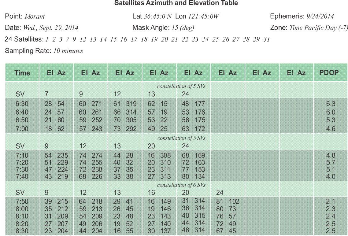
Ionospheric Delay
It is worth noting that the ionospheric error is usually smaller after sundown. In fact, the FGDC specified dual-frequency receivers for daylight observations for the achievement of the highest accuracies, due, in part, to the increased ionospheric delay during those hours. When planning the survey, it's always useful to note that the ionospheric error is smaller after sundown. The table above shows data from later in the day. It covers a period of two hours when a constellation of 5 and 6 satellites was always available. However, through the first hour, from 6:30 to 7:30, the PDOP hovered around 5 and 6. For the first half of that hour, four of the satellites—PRN 9, PRN 12, PRN 13, and PRN 24—were all near the same elevation. During the same period, PRN 9 and PRN 12 were only approximately 50° apart in azimuth, as well. Even though a sufficient constellation of satellites was constantly available, the survey designer may well have considered only the last 30 to 50 minutes of the time covered by this chart as suitable for observation. There is one caution, however. Azimuth-elevation tables are a convenient tool in the division of the observing day into sessions, but it should not be taken for granted that every satellite listed is healthy and in service. For the actual availability of satellites and an update on atmospheric conditions, it is always wise to check. In the planning stage, the diligence can prevent creation of a design dependent on satellites that prove unavailable. Similarly, after the field work is completed, it can prevent inclusion of unhealthy data in the postprocessing.
Supposing that the period from 7:40 to 8:30 was found to be a good window, the planner may have regarded it as a single 50-minute session, or divided it into shorter sessions. One aspect of that decision was probably the length of the baseline in question. In static GPS/GNSS, a long line of 30 km may require 50 minutes of 6-satellite data, but a short line of 3 km may not. Another consideration was probably the approximation of the time necessary to move from one station to another.
Drawing the Baselines

Horizontal Control
A good rule of thumb is to verify the integrity of the horizontal control by observing baselines between these stations first. The vectors can be used to both corroborate the accuracy of the published coordinates and later to resolve the scale, shift, and rotation parameters between the control positions and the new network that will be determined by GPS/GNSS. These baselines are frequently the longest in the project, and there is an added benefit to measuring them first. By processing a portion of the data collected on the longest baselines early in the project, the most appropriate length of the subsequent sessions can be found. This test may allow improvement in the productivity on the job without erosion of the final positions. By observing the horizontal control baselines first, you can discover any difficulty with the published coordinates. For example, if they are NGS brass caps, you would learn if there is any discrepancy with the published coordinates on these control stations.

Julian Day in Naming Sessions
The table in the illustration indicates that the name of the first session connecting the horizontal control is 49-1. The date of the planned session is given in the Julian system. Taken most literally, Julian dates are counted from January 1, 4713 B.C. However, most practitioners of GPS/GNSS use the term to mean the day of the current year measured consecutively from January 1. Under this construction, since there are 31 days in January, Julian day 49 is February 18. The designation 49-1 means that this is to be the first session on that day. Some prefer to use letters to distinguish the session. In that case, the label would be 49-A.
Independent Lines
This project will be done with four receivers. The table shows that receiver A will occupy point 1; receiver B, point 3; receiver C, point 8; and receiver D, point 13 in the first session. Where r is the number of receivers, every session yields r-1 independent baselines. That is why the illustration shows only three of the possible six base lines that will be produced by this arrangement. Only the independent, also known as nontrivial, lines are shown on the map. The three lines that are not drawn are called trivial, and are also known as dependent lines. This idea is based on restricting the use of the lines created in each observing session to the absolute minimum needed to produce a unique solution. In the planning stage, it is best to consider the shortest vectors independent and the three longest lines are eliminated as trivial, or dependent. That is the case with the session illustrated but it cannot be said that the shortest lines are always chosen to be the independent lines. Sometimes, there are reasons to reject one of the shorter vectors due to incomplete data, cycle slips, multipath, or some other weakness in the measurements. Before such decisions can be made, each session will require analysis after the data has actually been collected.
Another aspect of the distinction between independent and trivial lines involves the concept of error of closure, or loop closure. Loop closure is a procedure by which the internal consistency of a GPS/GNSS network is discovered. A series of baseline vector components from more than one GPS/GNSS session, forming a loop or closed figure, is added together. The closure error is the ratio of the length of the line representing the combined errors of all the vector’s components to the length of the perimeter of the figure. Any loop closures that only use baselines derived from a single common GPS/GNSS session will yield an apparent closure error of zero, because they are derived from the same simultaneous observations. For example, all the baselines between the four receivers in session 49-1 of the illustrated project will be based on ranges to the same GPS/GNSS satellites over the same period of time. Therefore, the trivial lines of 13- 1, 1-8, and 3-13 will be derived from the same information used to determine the independent lines of 1-3, 3-8, and 8-13. It follows that, if the fourth line from station 13 to station 1 were included to close the figure of the illustrated session, the error of closure would be zero. The same may be said of the inclusion of any of the trivial lines. Their addition cannot add any redundancy or any geometric strength to the lines of the session, because they are all derived from the same data. If redundancy cannot be added to a GPS/GNSS session by including any more than the minimum number of independent lines, how can the baselines be checked? Where does redundancy in GPS/GNSS work come from?
Redundancy
Redundancy means stations being measured more than once. It is a useful thing in trying to evaluate the accuracy or the correctness of a network.
If only two receivers were used to complete the illustrated project, there would be no trivial lines and it might seem there would be no redundancy at all. But to connect every station with its closest neighbor, each station would have to be occupied at least twice, and each time during a different session. For example, with receiver A on station 1 and receiver B on station 2, the first session could establish the baseline between them. The second session could then be used to measure the baseline between station 1 and station 4. It would certainly be possible to simply move receiver B to station 4 and leave receiver A undisturbed on station 1. However, some redundancy could be added to the work if receiver A were reset. If it were re-centered, re-plumbed, and its H.I. (height of instrument) re-measured, some check on both of its occupations on station 1 would be possible when the network was completed. Under this scheme, a loop closure at the end of the project would have some meaning. If one were to use such a scheme on the illustrated project and connect into one loop all of the 14 baselines determined by the 14 two-receiver sessions, the resulting error of closure would be useful. It could be used to detect blunders in the work, such as mis-measured H.I.s. Such a loop would include many different sessions. The ranges between the satellites and the receivers defining the baselines in such a circuit would be from different constellations at different times. On the other hand, if it were possible to occupy all 14 stations in the illustrated project with 14 different receivers simultaneously and do the entire survey in one session, a loop closure would be absolutely meaningless.
As soon as three or more receivers are considered, the discussion of redundant measurement must be restricted to independent baselines, excluding trivial lines. In the real world, such a project is not done with 14 receivers nor with 2 receivers, but with 3, 4, or 5. The achievement of redundancy takes a middle road. Redundancy is then defined by the number of independent baselines that are measured more than once, as well as by the percentage of stations that are occupied more than once. While it is not possible to repeat a baseline without reoccupying its endpoints, it is possible to reoccupy a large percentage of the stations in a project without repeating a single baseline. These two aspects of redundancy in GPS/GNSS - the repetition of independent baselines and the reoccupation of stations - are somewhat separate.

The illustration above shows one of the many possible approaches to setting up the baselines for this particular GPS/GNSS project. The design in the illustration shows lines in different colors showing the occupations using four GPS/GNSS receivers and how they are used through simultaneous occupation on these stations to create a network. The session numbers are in the table, the independent and trivial lines are listed. The A, B, C, and D receivers are shown and what points they occupy, at what stages. This is obviously done over 10 sessions over two consecutive days, and there's a good deal of redundancy in the network. However, that's simply the design. That doesn't mean that that's what will actually occur.
The survey design calls for the horizontal control to be occupied in session 49-1. It is to be followed by measurements between two control stations and the nearest adjacent project points in session 49-2. As shown in the table at the bottom of the figure, there will be redundant occupations on stations 1 and 3. Even though the same receivers will occupy those points, their operators will be instructed to reset them at a different H.I.s for the new session. A better, but probably less efficient, plan would be to occupy these stations with different receivers than were used in the first session.
Forming Loops
As the baselines are drawn on the project map for a static GPS/GNSS survey, or any GPS/GNSS work where accuracy is the primary consideration, the designer should remember that part of their effectiveness depends on the formation of complete geometric figures. When the project is completed, these independent vectors should be capable of formation into closed loops that incorporate baselines from two to four different sessions. In the illustrated baseline plan, no loop contains more than ten vectors, no loop in more than 100 km long, and every observed baseline will have a place in a closed loop.
Ties to the Vertical Control
The ties from the vertical control stations to the overall network are usually not handled by the same methods used with the horizontal control. The first session of the illustrated project was devoted to occupation of all the horizontal control stations. There is no similar method with the vertical control stations. First, the geoidal undulation would be indistinguishable from baseline measurement error. Second, the primary objective in vertical control is for each station to be adequately tied to its closest neighbor in the network. If a benchmark can serve as a project point, it is nearly always advisable to use it, as was done with stations 11 and 14 in the illustrated project. A conventional level circuit can often be used to transfer a reliable orthometric elevation from vertical control station to a nearby project point.
Finding the Number of Sessions
where
s = the number of observing sessions,
r = the number of receivers,
m = the total number of stations involved
Finding the Number of Sessions
The illustrated survey design calls for 10 sessions, but the calculation does not include human error, equipment breakdown, and other unforeseeable difficulties. It would be impractical to presume a completely trouble-free project. The FGCC proposed the following formula for arriving at a more realistic estimate. But n, p, and k require a bit more explanation. The variable n is a representation of the level of redundancy that has been built into the network, based on the number of occupations on each station. The illustrated survey design includes more than two occupations on all but 4 of the 14 stations in the network. In fact, 10 of the 14 positions will be visited three or four times in the course of the survey. There are a total of 40 occupations by the 4 receivers in the 10 planned sessions. By dividing 40 occupations by 14 stations, it can be found that each station will be visited an average of 2.857 times. Therefore, the planned redundancy represented by factor n is equal to 2.857 in this project.
The experience of a firm is symbolized by the variable p in the formula. The division of the final number of actual sessions required to complete past projects by the initial estimation yields a ratio that can be used to improve future predictions. That ratio is the production factor, p. A typical production factor is 1.1. A safety factor of 0.1, known as k, is recommended for GPS projects within 100 km of a company’s home base. Beyond that radius, an increase to 0.2 is advised.
The substitution of the appropriate quantities for the illustrated project increases the prediction of the number of observation sessions required for its completion:
In other words, the 2-day, 10-session schedule is a minimum period for the baseline plan drawn on the project map. A more realistic estimate of the observation schedule includes 14 sessions. It is also important to keep in mind that the observation schedule does not include time for on-site reconnaissance.
Static GPS/GNSS Control Surveying

The prospects for the success of a GPS/GNSS project are directly proportional to the quality and training of the people doing it. The handling of the equipment, the on-site reconnaissance, the creation of field logs, and the inevitable last-minute adjustments to the survey design all depend on the training of the personnel involved for their success. There are those who say the operation of GPS/GNSS receivers no longer requires highly qualified survey personnel. That might be true if effective GPS/GNSS surveying needed only the pushing of the appropriate buttons at the appropriate time. In fact, when all goes as planned, it may appear to the uninitiated that GPS/GNSS has made experienced field surveyors obsolete. But when the unavoidable breakdowns in planning or equipment occur, the capable people, who seemed so superfluous moments before, suddenly become indispensable. Also, the full range of conventional surveying equipment and expertise have a place in GPS/GNSS. For some, their role may be more abbreviated than it was formerly, but one element that can never be outdated is good judgment.

Conventional Equipment
Most GPS/GNSS projects require conventional surveying equipment for spirit-leveling circuits, offsetting horizontal control stations, and monumenting project points, among other things. It is perhaps a bit ironic that this most advanced surveying method also frequently has the need of the most basic equipment. The use of brush hooks, machetes, axes, and so forth, can sometimes salvage an otherwise unusable position by removing overhead obstacles. Another strategy for overcoming such hindrances has been developed, using various types of survey masts to elevate a separate GPS/GNSS antenna above the obstructing canopy. Flagging, paint, and the various techniques of marking that surveyors have developed over the years are still a necessity in GPS/GNSS work. The pressure of working in unfamiliar terrain is often combined with urgency. Even though there is usually not a moment to spare in moving from station to station, a GPS/GNSS surveyor frequently does not have the benefit of having visited the particular points before. In such situations, the clear marking of both the route and the station during reconnaissance is vital. Despite the best route marking, a surveyor may not be able to reach the planned station, or, having arrived, finds some new obstacle or unanticipated problem that can only be solved by marking and occupying an impromptu offset position for a session. A hammer, nails, shiners, paint, and so forth are essential in such situations.

Safety equipment
The high-visibility vests, cones, lights, flagmen, and signs needed for traffic control cannot be neglected in GPS/GNSS work. Unlike conventional surveying operations, GPS/GNSS observations are not deterred by harsh weather. Occupying a control station in a highway is dangerous enough under the best of conditions, but in the midst of a rainstorm, fog, or blizzard, it can be absolute folly without the proper precautions. And any time and trouble taken to avoid infraction of the local regulations regarding traffic management will be compensated by an uninterrupted observation schedule.
Communications
Whether the equipment is handheld or vehicle mounted, two-way radios and cell phones are used in most GPS/GNSS operations. However, the line of sight that is no longer necessary for the surveying measurements in GPS/GNSS is sorely missed in the effort to maintain clear radio contact between the receiver operators. A radio link between surveyors can increase the efficiency and safety of a GPS/GNSS project, but it is particularly valuable when last-minute changes in the observation schedule are necessary. When an observer is unable to reach a station, or a receiver suddenly becomes inoperable, unless adjustments to the schedule can be made quickly, each end of all of the lines into the missed station will require reobservation. The success of static GPS/GNSS hinges on all receivers collecting their data simultaneously. However, it is more and more difficult to ensure reliable communication between receiver operators in geodetic surveys, especially as their lines grow longer. High-wattage, private-line FM radios are quite useful when line of sight is available between them or when a repeater is available. The use of cell phones may eliminate the communication problem in some areas, but probably not in remote locations. Despite the limitations of the systems available at the moment, achievement of the best possible communication between surveyors on a GPS/GNSS project pays dividends in the long run.
Information
The information every GPS/GNSS observer carries throughout a project ought to include emergency phone numbers; the names, addresses, and phone numbers of relevant property owners; and the combinations to necessary locks. Each member of the team should also have a copy of the project map, any other maps that are needed to clarify position or access, and, perhaps most important of all, the updated observation schedule. The observation schedule for static GPS/GNSS work will be revised daily based upon actual production. It should specify the start–stop times and station for all the personnel during each session of the upcoming day. In this way, the schedule will not only serve to inform every receiver operator of his or her own expected occupations, but those of every other member of the project as well. This knowledge is most useful when a sudden revision requires observers to meet or replace one another.
| Svs PRNs | Session 1 Start 7:10 Stop 8:10 9, 12, 13, 16, 20, 24 |
8:10 to 8:40 |
Session 2 Start 8:40 Stop 9:50 3, 12, 13, 16, 20, 24 |
9:50 to 10:15 |
Session 3 Start 10:15 Stop 11:15 3, 12, 13, 16, 17, 20, 24 |
11:15 to 11:30 |
Session 4 Start 11:30 Stop 12:30 3, 16, 17, 20, 22, 23, 26 |
12:30 to 14:00 |
Session 5 Start 14:00 Stop 15:00 1, 3, 17, 21, 23, 26, 28 |
|---|---|---|---|---|---|---|---|---|---|
| Receiver A Dan H. |
Station 1 NGS Horiz. Control |
Re-Set | Station 1 NGS Horiz. Control |
Move | Station 5 NGS Benchmark |
Re-Set | Station 5 NGS Benchmark |
Re-Set | Station 5 NGS Benchmark |
| Receiver B Scott G. |
Station 3 NGS V&H Control |
Re-Set | Station 3 NGS V&H Control |
Move | Station 6 Project Point |
Re-Set | Station 6 Project Point |
Move | Station 1 NGS Horiz. Control |
| Receiver C Dewey A. |
Station 8 NGS Horiz. Control |
Move | Station 2 Project Point |
Re-Set | Station 2 Project Point |
Move | Station 7 Project Point |
Move | Station 10 NGS Benchmark |
| Receiver D Cindy E. |
Station 13 NGS Horiz. Control |
Move | Station 4 Project Point |
Re-Set | Station 4 Project Point |
Move | Station 9 Project Point |
Move | Station 13 NGS Horiz. Control |
This page shows an observation schedule for a static control survey. And as you see here, the sessions are numbered as to when they start and when they stop. And then the receiver A, B, C, and D is shown and what station they are to be on and what they are to do when they move from one to another. This sort of log is necessary when static surveying is done. Because, of course, the constellation needs to be observed simultaneously with GPS/GNSS receivers occupying the points here.
For example, receiver A on Station One, receiver B on Station Three, C on eight, and D on 13 and Session One need to be at that position beginning at 7:10 and stopping at 8:10 so that we will have a full hour of simultaneous observations on those stations. Then some reset and stay at the same place, and others move on to another station. For example, one and three reset, and Station 8 and 13 move. Station 8 moves to Station 2, Station 13 moves to Station 4. And then, of course, there's a half an hour given there for that move. And at 8:40, they all power up and observe till 9:50. This gives you an idea of how it is necessary to have the information of this well in hand when one does the work. This observation schedule can be revised, of course, if the observations don't go as planned. It should specify start and stop times. In this way, the schedule will not only serve to inform every receiver operator of his or her own expected occupations, but those of every other in the project as well. This is useful, sometimes, when unexpected occurrences cause a change in the schedule.
Station Data
Station Data Sheet

Click here to see a text description.
Station Data Sheet
Station Name: S 198 (Project 14)
USGS Quad: BEND
Year Monumented: 1945
Described by: S GRAHAM
Year Recovered: 2014
State/County: MONTANA/FLATHEAD COUNTY
stamp and sketch included
To Reach: The station is located about 9 miles southeast of the Dew Drop Inn and about 2 miles south of the Bend Guard Station. To reach from the Dew Drop Inn, go southeast from the junction of US Highway 2 and the Tee River Rd. (State Hwy. 20), 14 miles on the Tee River Road to a "4-Junction" with a Dim Road. Turn "left" (northwest) onto Dim Road and travel 6.1 miles to an abandoned windmill. The station is 80 feet north of the windmill, and 34 feet east of Dim Road.
Monument Description: Station mark is a standard metal disk set in a concrete post protruding three inches above the ground. The disk is stamped "S 198 1948"
Signature: S. Graham
Date: 2/17/14
The principles of good field notes have a long tradition in land surveying, and they will continue to have validity for some time to come. In GPS/GNSS, the ensuing paper trail will not only fill subsequent archives; it has immediate utility. For example, the station data sheet is often an important bridge between on-site reconnaissance and the actual occupation of a monument. Though every organization develops its own unique system of handling its field records, most have some form of the station data sheet. The document illustrated here is merely one possible arrangement of the information needed to recover the station. The station data sheet can be prepared at any period of the project, but perhaps the most usual times are during the reconnaissance of existing control or immediately after the monumentation of a new project point. Neatness and clarity, always paramount virtues of good field notes, are of particular interest when the station data sheet is to be later included in the final report to the client. The overriding principle in drafting a station data sheet is to guide succeeding visitors to the station without ambiguity. A GPS/GNSS surveyor on the way to observe the position for the first time may be the initial user of a station data sheet. A poorly written document could void an entire session if the observer is unable to locate the monument. A client, later struggling to find a particular monument with an inadequate data sheet, may ultimately question the value of more than the field notes.
Here is an example of a station data sheet. This is the sort of information that will be recorded again in a static control survey to show the station that has been occupied, show a sketch of where it is located relative to other fixed landmarks, and then other information—how to reach it, a description of the monument, and of course, a signature and a date.
Station name
The station name fills the first blank on the illustrated data sheet. Two names for a single monument is far from unusual. In this case the vertical control station, officially named S 198, is also serving as a project point, number 14. But two names purporting to represent the same position can present a difficulty. For example, when a horizontal control station is remonumented, a number 2 is sometimes added to the original name of the station, and it can be confusing. For example, it can be easy to mistake a station, "Thornton 2," with an original station named, "Thornton," that no longer exists. Both stations may still have a place in the published record, but with slightly different coordinates. Another unfortunate misunderstanding can occur when inexperienced field personnel mistake a reference mark, R.M., for the actual station itself. The taking of rubbings and/or close-up photographs are widely recommended to avoid such blunders regarding stations names or authority.

Station Rubbing
Source: https://slideplayer.com/slide/9394640/
Rubbings
The illustrated station data sheet provides an area to accommodate a rubbing. With the paper held on top of the monument’s disk, a pencil is run over it in a zigzag pattern, producing a positive image of the stamping. This method is a bit more awkward than simply copying the information from the disk onto the data sheet, but it does have the advantage of ensuring the station was actually visited and that the stamping was faithfully recorded. Such rubbings or close-up photographs are often required.
Photographs
The use of photographs is growing as a help for the perpetuation of monuments. It can be convenient to photograph the area around the mark as well as the monument itself. These exposures can be correlated with a sketch of the area. Such a sketch can show the spot where the photographer stood and the directions toward which the pictures were taken. The photographs can then provide valuable information in locating monuments, even if they are later obscured. Still, the traditional ties to prominent features in the area around the mark are the primary agent of their recovery. It's important to have an idea of exactly what the monument looked like and to ensure that the intended point was occupied.
Quad Sheet Name
Providing the name of the appropriate state, county, and USGS quad sheet helps to correlate the station data sheet with the project map. The year the mark was monumented, the monument description, the station name, and the "to-reach" description all help to associate the information with the correct official control data sheet and, most importantly, the correct station coordinates.
To-reach descriptions
When driving or walking to a position can be aided by computerized turn-by-turn navigation, it is a great tool that may make writing to-reach descriptions unnecessary. However, GPS/GNSS control work is often done in areas where the roadway mapping in such navigation aids is inadequate. In those situations, the description of the route to the station is one of the most critical documents written during the reconnaissance. Even though it is difficult to prepare the information in unfamiliar territory and although every situation is somewhat different, there are some guidelines to be followed. It is best to begin with the general location of the station with respect to easily found local features. The description in the top illustration relies on a road junction, a guard station, and a local business. After defining the general location of the monument, the description should recount directions for reaching the station. Starting from a prominent location, the directions should adequately describe the roads and junctions. Where the route is difficult or confusing, the reconnaissance team should not only describe the junctions and turns needed to reach a station; it is wise to also mark them with lath and flagging, when possible. It is also a good idea to note gates. Even if they are open during reconnaissance, they may be locked later. When turns are called for, it is best to describe not only the direction of the turn, but the direction of the new course too. For example, in the description in the station data sheet at the top, the turn onto the dim road from the Tee River Road is described to the,"left (northwest)." Roads and highways should carry both local names and designations found on standard highway maps. For example, in the illustrated form, Tee River Road is also described as State Highway 20. The "to-reach" description should certainly state the mileages, as well as the travel times where they are appropriate, particularly where packing-in is required. Land ownership, especially if the owner's consent is required for access, should be mentioned. The reconnaissance party should obtain the permission to enter private property and should inform the GPS/GNSS observer of any conditions of that entry. Alternate routes should be described where they may become necessary. It is also best to make special mention of any route that is likely to be difficult in inclement weather. Where helicopter access is anticipated, information about the duration of flights from point to point, the distance of landing sites from the station, and flight time to fuel supplies should be included on the station data sheet.
Flagging and Describing the Monument
Flagging the station during reconnaissance may help the observer find the mark more quickly. On the station data sheet, the detailed description of the location of the station with respect to roads, fence lines, buildings, trees, and any other conspicuous features should include measured distances and directions. A clear description of the monument itself is important. It is wise to also show and describe any nearby marks, such as reference monuments (R.M.'s) that may be mistaken for the station or aid in its recovery. The name of the preparer, a signature, and the date round out the initial documentation of a GPS/GNSS station.
Visibility Diagram and Satellites Azimuth/Elevation Tables

Click here to see a text description.
Station Visibility Diagram
Date: February 17, 2014
Station Name: S 198 (PROJECT 14)
Described By: S. GRAHAM
USGS Quad: BEND
Latitude: 47 degrees 52'39"
Longitude: 115 degrees 00'48"
radial diagram showing where the windmill is located
Comments: Obstruction from abandoned windmill south of the station as shown. Windmill base is cross-member steel.
Obstructions above the mask angle of a GPS/GNSS receiver must be taken into account in finalizing the observation schedule. A station that is blocked to some degree is not necessarily unusable, but its inclusion in any particular session is probably contingent on the position of the specific satellites involved.
It is important for GPS/GNSS observations to have a good view of the sky. Obstructions above the mask angle must be taken into account, especially with static control survey.
An Example
The diagram in the illustration is widely used to record such obstructions during reconnaissance. It is known as a station visibility diagram, a polar plot, or a skyplot. The concentric circles are meant to indicate 10° increments along the upper half of the celestial sphere, from the observer’s horizon at 0° on the perimeter, to the observer’s zenith at 90° in the center. The hemisphere is cut by the observer’s meridian, shown as a line from 0° in the north to 180° in the south. The prime vertical is signified as the line from 90° in the east to 270° in the west. The other numbers and solid lines radiating from the center, every 30° around the perimeter of the figure, are azimuths from north and are augmented by dashed lines every 10°.
Drawing obstructions
Using a compass and a clinometer, a member of the reconnaissance team can fully describe possible obstructions of the satellite’s signals on a visibility diagram. By standing at the station mark and measuring the azimuth and vertical angle of points outlining the obstruction, the observer can plot the object on the visibility diagram. For example, a windmill base is shown on in the illustration as a cross-hatched figure. It has been drawn from the observer's horizon up to 37° in vertical angle, from 168° to about 182° in azimuth at its widest point. This description by approximate angular values is entirely adequate for determining when particular satellites may be blocked at this station.
Once completed, this diagram allows you to correlate the obstructions shown with other charts that give you the number of satellites available, the azimuth and height of those satellites at a particular time. With all this information, you will be able to design the observation session on this particular point so that satellites will not be obstructed.
| Time | SV 3 Elev. |
SV 3 Azim. |
SV 12 Elev. |
SV 12 Azim. |
SV 13 Elev. |
SV 13 Azim. |
SV 20 Elev. |
SV 20 Azim. |
SV 24 Elev. |
SV 24 Azim. |
Elev. |
Azim. |
PDOP |
|---|---|---|---|---|---|---|---|---|---|---|---|---|---|
| 8:50 | 54 | 235 | 74 | 274 | 44 | 28 | 16 | 308 | 68 | 169 | 4.8 | ||
| 9:00 | 51 | 229 | 74 | 255 | 40 | 32 | 20 | 310 | 72 | 163 | 5.7 | ||
| 9:10 | 47 | 224 | 72 | 238 | 37 | 35 | 23 | 311 | 77 | 153 | 4.9 | ||
| 9:20 | 43 | 219 | 68 | 226 | 33 | 38 | 27 | 313 | 80 | 134 | 1.0 |
| Time | SV 3 Elev. |
SV 3 Azim. |
SV 12 Elev. |
SV 12 Azim. |
SV& 13 Elev. |
SV 13 Azim. |
SV 16 Elev. |
SV 16 Azim. |
SV 20 Elev. |
SV 20 Azim. |
SV 24 Elev. |
SV 24 Azim. |
PDOP |
|---|---|---|---|---|---|---|---|---|---|---|---|---|---|
| 9:30 | 39 | 215 | 64 | 218 | 29 | 41 | 16 | 179 | 31 | 314 | 81 | 102 | 2.1 |
| 9:40 | 35 | 212 | 59 | 213 | 26 | 45 | 19 | 176 | 36 | 314 | 80 | 73 | 2.3 |
| 9:50 | 31 | 209 | 54 | 209 | 23 | 48 | 23 | 173 | 40 | 315 | 76 | 57 | 2.4 |
| 10:00 | 27 | 207 | 49 | 206 | 19 | 52 | 27 | 170 | 44 | 314 | 72 | 49 | 2.5 |
| 10:10 | 23 | 204 | 44 | 204 | 16 | 55 | 30 | 167 | 48 | 314 | 67 | 45 | 2.5 |
For example, suppose a 1-hour session from 9:10 to 10:10, illustrated in this table, was under consideration for the observation on station S 198. The station visibility chart might motivate a careful look at space vehicle (SV) pseudorandom noise (PRN) 16. Twenty minutes into the anticipated session, at 9:30 SV 16 has just risen above the 15° mask angle. Under normal circumstances, it would be available at station S 198, but it appears from the polar plot that the windmill will block its signals from reaching the receiver. In fact, the signals from SV 16 will apparently not reach station S 198 until sometime after the end of the session at 10:10.
Working around Obstructions
Under the circumstances, some consideration might be given to observing station S 198 during a session when none of the satellites would be blocked. However, the 9:10 to 10:10 session may be adequate after all. Even if SV 16 is completely blocked, the remaining 5 satellites will be unobstructed, and the constellation still will have a relatively low position dilution of precision (PDOP). Still, the analysis must be carried to other stations that will be occupied during the same session. The success of the measurement of any baseline depends on common observations at both ends of the line. Therefore, if the signals from SV 16 are garbled or blocked from station S 198, any information collected during the same session from that satellite at the other end of a line that includes S 198 will be useless in processing the vector between those two stations.
However, the material of the base of the abandoned windmill has been described on the visibility diagram as cross-membered steel, so it is possible that the signal from SV 16 will not be entirely obstructed during the whole session. There may actually be more concern of multipath interference from the structure than that of signal availability. One strategy for handling the situation might be to program the receiver at S 198 to ignore the signal from SV 16 completely if the particular receiver allows it. The visibility diagram and the azimuth-elevation table complement each other. They provide the field supervisor with the data needed to make informed judgments about the observation schedule. Even if the decision is taken to include station S 198 in the 9:10 to 10:10 session as originally planned, the supervisor will be forewarned that the blockage of SV 16 may introduce a bit of weakness at that particular station.
Multipath

The multipath condition is by no means unique to GPS/GNSS. When a transmitted television signal reaches the receiving antenna by two or more paths, the resulting variations in amplitude and phase cause the picture to have ghosts. This kind of scattering of the signals can be caused by reflection from land, water, or man-made structures. In GPS/GNSS, the problem can be particularly troublesome when signals are received from satellites at low elevation angles; hence, the general use of a 15° to 20° mask angle. The use of choke ring antennas to mediate multipath may also be considered. It is also wise, where it is possible, to avoid using stations that are near structures likely to be reflective or to scatter the signal. For example, chain-link fences that are found hard against a mark can cause multipath by forcing the satellite’s signal to pass through the mesh to reach the antenna. The elevation of the antenna over the top of the fence with a survey mast is often the best way to work around this kind of obstruction. Metal structures with large flat surfaces are notorious for causing multipath problems. A long train moving near a project point could be a potential problem, but vehicles passing by on a highway or street usually are not, especially if they go by at high speed. It is important, of course, to avoid parked vehicles. It is best to remind new GPS/GNSS observers that the survey vehicle should be parked far enough from the point to avert any multipath. A good way to handle these unfavorable conditions is to set an offset point.
Avoiding obstructions is a significant part of planning and performing a good GPS/GNSS observation.
Point Offsets

An offset must, of course, stand far enough away from the source of multipath or an attenuated signal to be unaffected. However, the longer the distance from the originally desired position, the more important the accuracy of the bearing and distance between that position and the offset becomes. Recording the tie between the two correctly is crucial to avoid misunderstanding after the work is completed. Some receivers allow input of the information directly into the observations recorded in the receiver or data logger. However, during a control survey, it is best to also record the information in a field book. Offsets in GPS/GNSS control surveying are an instance where conventional surveying equipment and expertise are necessary. Clearly, the establishment of the tie requires a position for the occupation of the instrument, i.e. a total station, and a position for the establishment of its orientation, that is, an azimuth. It is best to establish three intervisible rather than two points—one to occupy and two azimuth marks. This approach makes it possible to add a redundant check to the tie. The positions of these two, or three, points may be established by setting monuments and performing static observations on them all. Alternatively, azimuthal control may be established by astronomic observations.
Monumentation

The monumentation set for GPS/GNSS projects varies widely and can range from brass tablets to aerial premarks, capped rebar or even pin flags. The objective of most station markers is to adequately serve the client's subsequent use. However, the time, trouble, and cost in most high-accuracy GPS/GNSS work warrants the most permanent, stable monumentation. Many experts predict that GPS/GNSS will eventually make monumentation unnecessary. The idea foresees GPS/GNSS receivers in constant operation at well-known master (i.e. CORS) stations will allow surveyors with receivers to determine highly accurate relative positions with such speed and ease that monumentation will be unnecessary. The idea may prove prophetic, but, for now, monumentation remains an important part of most GPS/GNSS projects. The suitability of a particular type of monument is an area still most often left to the professional judgement of the surveyors involved.
Observation

When everything goes as planned, a GPS/GNSS observation is uneventful. However, even before the arrival of the receiver operator at the control or project point, the session can get off-track. The simultaneity of the data collected at each end of a baseline is critical to the success of any measurement in static GPS/GNSS control surveys. When a receiver occupies a master station throughout a project, there need be little concern on this subject. But most static applications depend on the sessions of many mobile receivers beginning and ending together.
Arrival
The number of possible delays that may befall an observer on the way to a station are too numerous to mention. With proper planning and reconnaissance, the observer will likely find that there is enough time for the trip from station to station and that sufficient information is on hand to guide the observer to the position, but this, too, cannot be guaranteed. When the observer is late to the station, the best course is usually to set up the receiver quickly and collect as much data as possible. The baselines into the late station may or may not be saved, but they will certainly be lost if the receiver operator collects no information at all. It is at times like these that good communication between the members of the GPS/GNSS team is most useful. For example, some of the other observers in the session may be able to stay on their station a bit longer with the late arrival and make up some of the lost data. Along the same line, it is usually a good policy for those operators who are to remain on a station for two consecutive sessions to collect data as long as possible, while still leaving themselves enough time to reset between the two observation periods.
Set-up
Centering an instrument over the station mark is always important. However, the centimeter-level accuracy of static GPS/GNSS gives the centering of the antenna special significance. It is ironic that such a sophisticated system of surveying can be defeated from such a commonplace procedure. A tribrach with an optical plummet or any other device used for centering should be checked and, if necessary, adjusted before the project begins. With good centering and leveling procedures, an antenna should be within a few millimeters of the station mark. Unfortunately, the centering of the antenna over the station does not ensure that its phase center is properly oriented. The contours of equal phase around the antenna’s electronic center are not themselves perfectly spherical. Part of their eccentricity can be attributed to unavoidable inaccuracies in the manufacturing process. To compensate for some of this offset, it is a good practice to rotate all antennas in a session to the same direction. Many manufacturers provide reference marks on their antennas so that each one may be oriented to the same azimuth. That way, they are expected to maintain the same relative position between their physical and electronic centers when observations are made.
Height of Instrument

The care ascribed to the measurement of antenna heights is due to the same concern applied to centering. GPS/GNSS has an extraordinary capability to achieve accurate ellipsoidal heights, but those heights can be easily contaminated by incorrect H.I.s.
Most GPS/GNSS receivers capable of geodetic accuracy are designed to be mounted on a tripod, usually with a tribrach and adaptor. However, there is a trend toward bipod- or range-pole-mounted antennas. An advantage of these devices is that they ensure a constant height of the antenna above the station. The mismeasured height of the antenna above the mark is probably the most pervasive and frequent blunder in GPS/GNSS control surveying. The tape or rod used to measure the height of the antenna is sometimes built into the receiver and sometimes a separate device. It is important that the height of the instrument (H.I.) be measured accurately and consistently in both feet and meters, without merely converting from one to the other mathematically. It is also important that the value be recorded in the field notes and, where possible, also entered into the receiver itself. Since many systems measure the height of the antenna to the edge of the ground plane or to the exterior of the receiver itself, the calibration of the tribrach affects both the centering and the H.I. measurement. The resetting of a receiver that occupies the same station in consecutive sessions is an important source of redundancy for many kinds of GPS/GNSS networks. However, integrity can only be added if the tribrach has been accurately calibrated.

The measurement of the height of the antenna in a GPS/GNSS survey is often not made on a plumb line. A tape is frequently stretched from the top of the station monument to some reference mark on the antenna or the receiver itself. Some GPS/GNSS teams measure and record the height of the antenna to more than one reference mark on the ground plane. These measurements are usually mathematically corrected to plumb.
Observation Logs

The most immediate use of the observation log is an evaluation of the day's work. Most GPS/GNSS control survey operations require its receiver operators to keep a careful log of each observation. Usually written on a standard form, these field notes provide a written record of the measurements, times, equipment, and other data that explains what actually occurred during the observation itself. It is difficult to overestimate the importance of this information. It is usually incorporated into the final report of the survey, the archives, and any subsequent effort to blue-book the project. However, the most immediate use of the observation log is in evaluation of the day's work by the on-site field supervisor. An observation log may be organized in a number of ways. The log illustrated is one method that includes some of the information that might be used to document one session at one station. Of course, the name of the observer and the station must be included, and while the date need not be expressed in both the Julian and Gregorian calendars, that information may help in quick cataloging of the data. The approximate latitude, longitude, and height of the station are usually required by the receiver as a reference position for its search for satellites. The date of the planned session will not necessarily coincide with the actual session observed. The observer's arrival at the point may have been late, or the receiver may have been allowed to collect data beyond the scheduled end of the session. There are various methods used to name the observation session in terminology that is sensible to computers. A widely used system is noted here. The first four digits are the project point’s number. In this case, it is point 14 and is designated 0014. The next three digits are the Julian day of the session, in this case it is day 50, or 050. Finally, the session illustrated is the second of the day, or 2. Therefore, the full session name is 0014 050 2. Whether onboard or separate, the type of the antenna used and the height of the antenna are critical pieces of information. The relation of the height of the station to the height of the antenna is vital to the station’s later utility. The distance that the top of the station's monument is found above or below the surface of the surrounding soil is sometimes neglected. This information can not only be useful in later recovery of the monument, but can also be important in the proper evaluation of photo-control panel points.
Weather
The meteorological data is useful in modeling the atmospheric delay. Measurement of the atmospheric pressure in millibars, the relative humidity, and the temperature in degrees Centigrade are sometimes expected to be in the observation log. However, the general use is less stringent. The conditions of the day are observed, and unusual changes in the weather are noted. A record of the satellites that are actually available during the observation and any comments about unique circumstances of the session round out the observation log.
Daily Progress Evaluation

The planned observation schedules of a large GPS/GNSS project usually change daily. The arrangements of upcoming sessions are often altered based on the success or failure of the previous day’s plan. Such a regrouping follows an evaluation of the day’s data. This evaluation involves examination of the observation logs as well as the data each receiver has collected. Unhealthy data, caused by cycle slips or any other source, are not always apparent to the receiver operator at the time of the observation. Therefore, a daily quality control check is a necessary preliminary step before finalizing the next day’s observation schedule. Some field supervisors prefer to compute the independent baseline vectors of each day’s work to ensure that the measurements are adequate. Obviously, if a vector has failed, it's important to know it the very day it occurred so that it can be picked up in the subsequent day or days. Neglecting the daily check could leave unsuccessful sessions undiscovered until the survey was thought to be completed. The consequences of such a situation could be expensive.
Online Post-Processing Services

Using a Processing Service
An alternative to in-house post-processing is the use of a processing service. There are several services available to GPS/GNSS surveyors. While they differ somewhat in their requirements, they are all based on the same idea. Static GPS/GNSS data collected in the field may be uploaded to a website on the Internet by the hosting organization, which will then return the final positions, often free of charge. Usually, the user is directed to an ftp site where the results can be downloaded. There can be advantages to the use of such a processing service. Aside from removing the necessity of having post-processing software in-house, there is the strength of the network solution available from them. In other words, rather than the data sent in by the GPS/GNSS surveyor being processed against a single CORS in the vicinity of the work, it is processed against a group of the nearest CORS. There are often three in the group. Such a network-based solution improves the integrity of the final position markedly and may compensate for long baselines required by the sparseness of the CORS in the area of interest. Among the online resources available for processing services is the National Geodetic Survey's Online Positioning User Service (OPUS). This service allows the user to submit RINEX files through NGS' Web page. They are processed automatically with NGS computers and software utilizing data from three CORS that may be user selected. There are others, such as the Australian Online GPS Processing Service, AUSPOS.
Post-computed Ephemerides

This system is augmented by other tracking networks that produce post-computed ephemerides. Their impetus have been several: the necessity of timely orbital information with more precision than the broadcast ephemeris and the correlation of the terrestrial coordinate systems with the orbital system through VLBI and SLR sites, among others. Since the monitoring stations are tracking the actual satellites all the time, it is possible this tracking information can be used to produce ephemerides of the actual position of the satellite at the time you were observing it. In other words, given a position on the Earth and given a window of time, it is possible for you to go on the Internet and download from these sites the precise ephemeris, the post-computed ephemeris, of the moment at which you were observing the satellite. It's valuable, of course, because the broadcast ephemeris is not as accurate as the tracking information of the actual satellites you're observing at the time you're observing them. The broadcast ephemeris is predictive of where the satellite will be later. It is much different to have the tracking information of the satellite at the moment you were tracking it with your receiver.
The following ephemeris categories and the time they are available after tracking (latency) can be found at NOAAs GPS Orbit Data site
Ultra-rapid (iguWWWWD.sp3)
6-hour latency
constrained (no-net rotation, no-net translation) 24-hour file – sp3
Rapid (igrWWWWD.sp3)
13-hour latency
constrained (no-net rotation, no-net translation) 24-hour file – sp3
Final (igsWWWWD.sp3)
12 to 14 day latency
minimally constrained (no-net rotation) 24 hour file - sp3
Discussion
Discussion Instructions
To continue the discussion begun by this lesson, I would like to pose this question:
In a properly designed static GPS/GNSS survey would a loop closure include independent or dependent baselines? What is the difference between independent and dependent baselines? Why is redundancy a good thing in GPS/GNSS work?
To participate in the discussion, please go to the Lesson 7 Discussion Forum in Canvas. (That forum can be accessed at any time by going to the GEOG 862 course in Canvas and then looking inside the Lesson 7 module.)
Summary

So, here are the fundamental ideas that underlie the static GPS/GNSS surveying technique. The first receiver, the base, provides the data to compute the differences between its known position and the unknown positions measured at the second, or roving receiver. Static GPS/GNSS requires post-processing and is used for establishing control by GPS/GNSS. While correlated systematic errors can be virtually eliminated with differential correction, the biases such as multipath and receiver channel noise are certainly not. These errors have been much reduced in modern GPS/GNSS receivers, but not completely defeated. Biases such as high PDOP can only be resolved with both good receiver design and care as to when and where the surveying is done.
In the next lesson, we delve into real-time GPS/GNSS work and Precise Point Positioning.
Before you go on to Lesson 8, double-check the Lesson 7 Checklist to make sure you have completed all of the activities listed there.
Lesson 8: Real-Time Global Positioning System Surveying
The links below provide an outline of the material for this lesson. Be sure to carefully read through the entire lesson before returning to Canvas to submit your assignments.
Lesson 8 Overview
Overview
Most, not all, GPS surveying relies on the idea of differential positioning. The mode of a base or reference receiver at a known location logging data at the same time as a receiver at an unknown location together provide the fundamental information for the determination of accurate coordinates. While this basic approach remains today, the majority of GPS surveying is not done in the static post-processed mode. Post-processing is most often applied to control work. Now, the most commonly used methods utilize receivers on reference stations that provide correction signals to the end user via a data link sometimes over the Internet, radio signal, or cell phone and often in real-time.
Objectives
At the successful completion of this lesson, students should be able to:
- explain the uses of real-time kinematic GPS/GNSS and DGPS/GNSS;
- describe WAAS;
- define RTCM SC-104;
- recognize the use of the radio licensing and cell phones in RTK;
- recognize some practical RTK suggestions; and
- recognize precise point positioning PPP.
Questions?
If you have any questions now or at any point during this week, please feel free to post them to the Lesson 8 Discussion Forum. (To access the forum, return to Canvas and navigate to the Lesson 8 Discussion Forum in the Lesson 8 module.) While you are there, feel free to post your own responses if you, too, are able to help out a classmate.
Checklist
Lesson 8 is one week in length. (See the Calendar in Canvas for specific due dates.) To finish this lesson, you must complete the activities listed below. You may find it useful to print this page out first so that you can follow along with the directions.
| Step | Activity | Access/Directions |
|---|---|---|
| 1 | Read the lesson Overview and Checklist. | You are in the Lesson 8 online content now. The Overview page is previous to this page, and you are on the Checklist page right now. |
| 2 | Read the Chapter 7 in GPS for Land Surveyors. | Text |
| 3 | Read the lecture material for this lesson. | You are currently on the Checklist page. Click on the links at the bottom of the page to continue to the next page, to return to the previous page, or to go to the top of the lesson. You can also navigate the lecture material via the links in the Lessons menu. |
| 4 | Participate in the Discussion. | To participate in the discussion, please go to the Lesson 8 Discussion Forum in Canvas. (That forum can be accessed at any time by going to the GEOG 862 course in Canvas and then looking inside the Lesson 8 module.) |
| 5 | Read lesson Summary. | You are in the Lesson 8 online content now. Click on the "Next Page" link to access the Summary. |
Real-Time Kinematic and Differential GPS

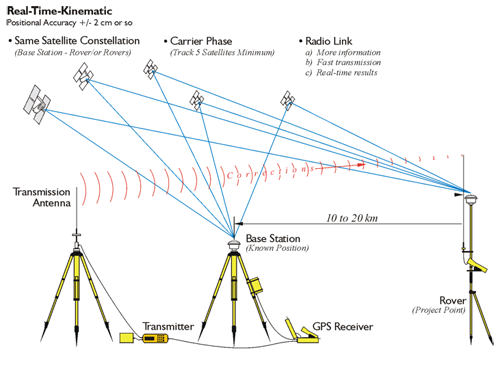
Errors in satellite clocks, imperfect orbits, the trip through the layers of the atmosphere, and many other sources contribute inaccuracies to GPS/GNSS signals by the time they reach a receiver. Real-time positioning is built on the idea that, with the important exceptions of multipath and receiver noise, these GPS/GNSS error sources are correlated. Nevertheless, the errors are variable, so the best to way to correct them is to monitor them as they happen. A good way to do this is to set up a GPS/GNSS receiver on a station whose position is known exactly, a base station. This base station receiver’s computer can calculate its position from satellite data, compare that position with its actual known position, and find the difference. The resulting error corrections can be communicated from the base to the rover over a data link. It works well, as long as the base station monitors them all the time, at least all the time the rover receiver or receivers are working. While this is happening, the rovers move from place to place collecting the points whose positions you want to know relative to the base station, which is the real objective after all.

Radial GPS/GNSS
Such real-time surveying is essentially radial. There are advantages to the approach. The advantage is a large number of positions can be established in a short amount of time with little or no planning. The disadvantage is that there is little or no redundancy in positions derived, each of the baselines originates from the same control station. If there's an error in one of these radial baselines, it would be tough to catch it because there's no real redundancy. Redundancy can be incorporated, but it requires repetition of the observations so each baseline is determined with more than one GPS/GNSS constellation. One way to do it is to occupy the project points, the unknown positions, successively, with more than one rover. It is best if these successive occupations are separated by 4 hours and not more than 8 hours, so the satellite constellation can reach a significantly different configuration. However, a re-occupation as little as 1/2 hour later can yield good results. Another way is to move the base to another known point. Then, if you have vectors from another base into these points, you have a check. This approach allows a solution to be available from two separate control stations. Obviously, this can be done with re-occupation of the project points after one base station has been moved to a new control point, or a two base stations can be up and running from the very outset and throughout of the work as would be the case using two CORS stations. An advantage to a continuously operating reference station network is that since those bases are operating simultaneously and all the time, it's possible to download the positions from more than one base and process your new position based on these continuously operating reference stations and have some redundancy.
A more convenient but less desirable approach is to do a second occupation almost immediately after the first. The roving receiver’s antenna is blocked or tilted until the lock on the satellites is interrupted. It is then re-oriented on the unknown position a second time for the repeat solution. This does offer a second solution, but from virtually the same constellation.
Project points that are near one another but far from the control station should be directly connected with a baseline to maintain the integrity of the survey. Finally, if the base receiver loses lock and it goes unnoticed, it will completely defeat the radial survey for the time it is down.
Differential GPS (DGPS)

The term DGPS is sometimes used to refer to differential GPS that is based on pseudoranges, aka code phase. Even though the accuracy of code phase applications was given a boost with the elimination of Selective Availability (SA) in May 2000, consistent accuracy better than the 2-5 meter range still requires reduction of the effect of correlated ephemeris and atmospheric errors by differential corrections. Though the corrections could be applied in post-processing services that supply these corrections, most often operate in real-time. In such an operation, pseudorange based versions can offer meter- or even submeter results. Usually, pseudorange corrections are broadcast from the base to the rover or rovers for each satellite in the visible constellation. Rovers with an appropriate input/output (I/O) port can receive the correction signal and calculate coordinates. The real-time signal comes to the receiver over a data link. It can originate at a project specific base station, or it can come to the user through a service, of which there are various categories. Some are open to all users, and some are by subscription only. Coverage depends on the spacing of the beacons, aka transmitting base stations, their power, interference, and so forth. Some systems require two-way, some one-way, communication with the base stations. Radio systems, geostationary satellites, low-earth-orbiting satellites and cellular phones are some of the options available for two-way data communication. In any case, most of the wide variety of DGPS services were not originally set up to augment surveying and mapping applications of GPS; they were established to aid GPS navigation.
Real-Time Kinematic

The Correction Signal
The agreed upon protocol for communication between base stations and rovers was first designed for used in marine navigation by an organization known as the Radio Technical Commission for Maritime Services (RTCM). RTCM is an independent not-for-profit organization that is supported by an international membership that includes both governmental and non-governmental institutions. Its goals are educational, scientific, and professional. Toward those ends, it provides information on maritime radio-navigation and radio communication policies and associated regulations to its members. It is also involved in technical standards development.
In 1985, the RTCM Special Committee (SC-104) created a standard that is still more used than any proprietary formats that have come along since. RTCM is open. In other words, it is a general-purpose format and is not restricted to a particular receiver type. The message augments the information from the satellites. It was originally designed to accommodate a slow GPS data rate with a configuration somewhat similar to the navigation message. The data format has evolved since its inception. For example, RTCM 2.0 supported GPS code only. However, when it became clear in 1994 that including carrier phase information in the message could improve the accuracy of the system, RTCM Special Committee 104 added four new message types to Version 2.1 to fulfill the needs of RTK. RTCM 2.1 supported both code and phase correction, but still GPS only. Version 2.2 became available in 1998. RTCM 2.2 added support for GLONASS, and version 2.3 included antenna corrections, and the changes continued. In 2007, the Radio Technical Commission for Maritime Services Special Committee 104 published its Version 3. RTCM 3.0 utilizes a more efficient message structure than its predecessors, which proves beneficial in the RTK data heavy real-time communications between a base and a rover. Version 3.0 still provides both GPS and GLONASS code and carrier messages, antenna and system parameters. RTCM 3.1 adds a network correction message and version 3.2 announced in 2013 introduces a feature known as Multiple Signal Messages (MSM). MSM includes the capability to handle the European Galileo and the Chinese Beidou GNSS systems in the RTCM protocol.
Satellite Based Augmentation

The correlation between most of the GPS biases becomes weaker as the rover gets farther from the base. The term Local Area Differential GPS (LADGPS), is used when the baselines from a single base station to the roving receivers using the service are less than a couple of hundred kilometers. The term Wide Area Differential GPS (WADGPS) is used when the service uses a network of base stations and distributes correction over a larger area, an area that may even be continental in scope. Many bases operating together provide a means by which the information from several of them can be combined to send a normalized or averaged correction tailored to the rover’s geographical position within the system. Some use satellites to provide the data link between the service provider and the subscribers. Such a system depends on the network of base stations on the ground receiving signals from the GPS/GNSS constellation and then streaming that data to a central computer at a control center. Then the corrections are calculated and uploaded to a geo-stationary communication satellite. You see that on the left with the yellow arrow going up as an upload to a satellite, Inmarsat. The satellite then broadcasts these correction signals to the service’s subscribers (i.e. aircraft).
NDGPS Coverage and Wide Area Augmentation System (WAAS)

NDGPS
Both the U.S. Coast Guard (USCG) and the Canadian Coast Guard (CCG) instituted DGPS services to facilitate harbor entrances, ocean mapping, and marine traffic control as well as navigation in inland waterways. Their system base stations beacons broadcast GPS corrections along major rivers, major lakes, the east coast, and the west coast. The sites use marine beacon frequencies of 255 to 325 kHz, which has the advantage of long range propagation that can be several hundreds of kilometers. Access to the broadcasts is free, and over recent years the service has become very popular outside of its maritime applications, particularly among farmers engaged in GPS aided precision agriculture. Therefore, the system has been extended beyond waterways across the continental U.S. and is now known as the Nationwide DGPS (NDGPS).
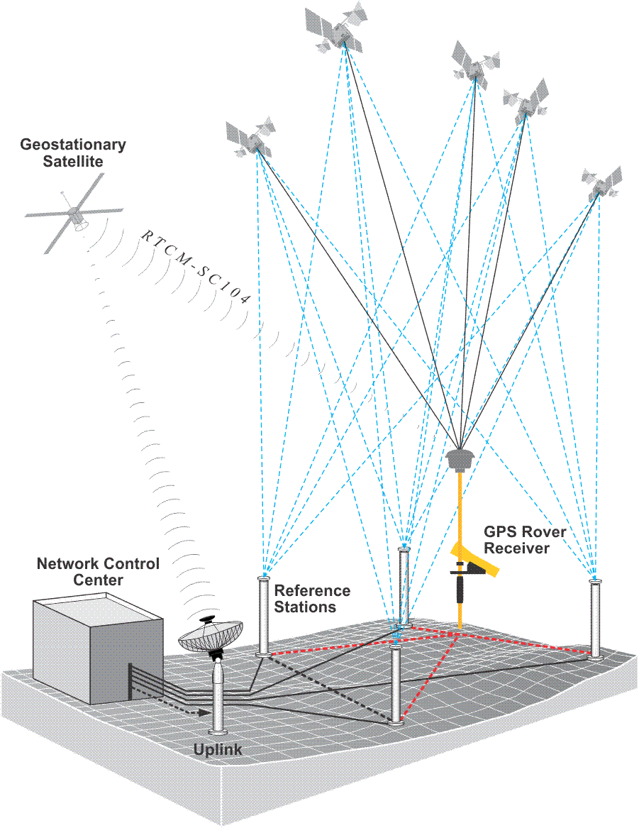
Wide Area Augmentation System, WAAS
Another U.S. DGPS service initiated in 1994 cooperatively by the Department of Transportation and the Federal Aviation Administration (FAA) is known as WAAS (see figure above). It is available to users with GPS receivers equipped to receive it. The signal is free. The official horizontal accuracy is 7.6 m, but it often delivers better. It utilizes both satellite-based augmentation systems, also known as SBAS, and ground-based augmentations and was initially designed to assist aerial navigation from takeoff, en route through landing. Reference stations at known locations are the bases on the ground. They send their data via processing sites to three Ground Earth Master Stations that upload differential corrections and time to three commercial geo-stationary satellites devoted to transmission of GPS differential corrections to users on the ground. DGPS requires that all receivers collect pseudoranges from the same constellation of satellites. It is vital that the errors corrected by the base station are common to the rovers. The rover must share its selection of satellites with the base station.
The European Geostationary Navigation Overlay Service (EGNOS) has a similar configuration as does the Japanese Multi-functional Satellite Augmentation System (MSAS); India's GPS And Geo-Augmented Navigation (GAGAN) system and Russia's System for DIfferential Corrections and Monitoring (SDCM).
Latency and GIS

Latency
It takes some time for the base station to calculate corrections, and it takes some time for it to put the data into packets in the correct format and transmit them. Then the data makes its way from the base station to the rover over the data link. It is decoded and must go through the rover’s software. The time this takes is called the latency of the communication between the base station and the rover. It can be as little as a quarter of a second or as long as a couple of seconds. And since the base station's corrections are only accurate for the moment they were created, the base station must send a range rate correction along with them. Using this rate correction, the rover can back date the correction to match the moment it made that same observation.
Identical Constellation
DGPS requires that all receivers collect pseudoranges from the same constellation of satellites. It is vital that the errors corrected by the base station are common to the rovers. The rover must share its selection of satellites with the base station; otherwise it would be necessary to create differential corrections for all the combinations of all the available satellites. That could get unmanageable in a hurry, for example, with just four satellites above the observer’s horizon, there can be more than 80 such combinations.
GIS Applications for DGPS
Aerial navigation, marine navigation, agriculture, vehicle tracking, and construction utilize DGPS. DGPS is also useful in land and hydrographic surveying, but perhaps the fastest growing application for DGPS is in data collection, data updating, and even in-field mapping for Geographic Information Systems (GIS). GIS data has long been captured from paper records, such as digitizing and scanning paper maps. Photogrammetry, remote sensing, and conventional surveying have also been data sources for GIS. More recently, data collected in the field with DGPS has become significant in GIS.
GIS data collection with DGPS requires the integration of the position of features of interest and relevant attribute information about those features. In GIS, it is frequently important to return to a particular site or feature to perform inspections or maintenance. DGPS with real-time correction makes it convenient to load the position or positions of features into a data logger, and navigate back to the vicinity. But to make such applications feasible, a GIS must be kept current. It must be maintained. A receiver configuration including real-time DGPS, sufficient data storage, and graphic display allows verification and updating of existing information.
DGPS allows the immediate attribution and validation in the field, with accurate and efficient recording of position. In the past, many GIS mapping efforts have often relied on ties to street centerlines, curb-lines, railroads, and so forth. Such dependencies can be destroyed by demolition or new construction. DGPS can provide reliable positioning even if the landscape has changed. And its data can be integrated with other technologies, such as laser range-finders, and so forth, in environments where DGPS is not ideally suited to the situation. Finally, loading GPS/GNSS data into a GIS platform does not require manual intervention. GPS/GNSS data processing can be automated; the results are digital and can pass into a GIS format without redundant effort, reducing the chance for errors.
RTK and the Federal Communications Commission (FCC)
Kinematic surveying, also known as stop-and-go kinematic surveying, is not new. The original kinematic GPS/GNSS innovator, Dr. Benjamin Remondi, developed the idea in the mid-1980s. Real-Time Kinematic, RTK, is a method that provides positional accuracy nearly as good as static carrier phase positioning, but faster. RTK accomplishes positioning in real-time shown in the figure above. It involves the use of at least one stationary reference receiver, the base station, and at least one moving receiver, the rover. All the receivers involved observe the same satellites simultaneously. The base receivers are stationary on control points. The rovers move from project point to project point across, stopping momentarily at each new point, usually briefly. The collected data provides vectors between themselves and the base receivers in real-time. RTK has become routine in development and engineering surveys where the distance between the base and roving receivers can most often be measured in thousands of feet. When compared with the other relative positioning methods, there is little question that the very short sessions of the real-time kinematic method can produce the largest number of positions in the least amount of time. The remarkable thing is that this technique can do so with only slight degradation in the accuracy of the work. Real-time kinematic is done by carrier phase ranging. It must track five satellites minimum. The reason for the five satellites is basically to have one spare so that you're absolutely sure that you will have a position all the time. The base station is set up on a known point there is a transmission antenna associated with it through which a radio transmitter sends corrections to a rover. The baselines are typically at 10 to 20 kilometers, which is considerably shorter than DGPS's effective range.
Fixing the Integer Ambiguity in RTK
RTK receivers can be single- or multi-frequency receivers with GPS/GNSS antennas, but multi-frequency receivers are usual because RTK relies on carrier phase observations corrected in real-time. In other words, it depends on the fixing of the integer cycle ambiguity, and that is most efficiently accomplished with a multi-frequency GPS/GNSS receiver capable of making both carrier phase and precise pseudorange measurements. Here is one way it can be done. A search area is defined in the volume of the possible solutions, but that group is narrowed down quite a bit by using pseudoranges. If the number of integer combinations to be tested is greatly reduced with precise pseudoranges, the search can be quickly limited. The possible solutions in that volume are tested statistically, according to a minimal variance criterion, and the best one is found. This candidate is verified, that is, compared with the second best candidate. The process can take less than 10 seconds under the best circumstances where the receivers are tracking a large constellation of satellites, the PDOP is small, the receivers are multi-frequency, there is no multipath, and the receiver noise is low. This technique relies on multi-frequency information. Observations are combined into a wide lane, which has an ambiguity of about 86 cm, and the integer ambiguity is solved in a first pass. This information is used to determine the kinematic solution on L1. Therefore, it is a good idea to restrict RTK to situations where there is good correlation of atmospheric biases at both ends of the baseline. In other words, RTK is best used when the distance between the base and rover is between 10 km and 20 km, 6 miles and 12 miles, but usually less. It is fortunate that GPS/GNSS receivers with virtually instantaneous carrier phase-based positioning are available. These techniques of integer cycle ambiguity resolution, validation, and quality control are being further improved to apply to GNSS data processing.
![]()
RTK also requires a real-time wireless connection be maintained between the base station and the rover. The radio receiving antennas for the rovers will either be built into the GPS/GNSS antenna or be present as separate units. It is usual that the radio antenna for the data transmitter and the rover are omnidirectional whip antennas; however, at the base it is usually on a separate mast and has a higher gain than those at the rovers. The position of the transmitting antenna affects the performance of the system significantly. It is usually best to place the transmitter antenna as high as is practical for maximum coverage, and the longer the antenna, the better its transmission characteristics. It is also best if the base station occupies a control station that has no overhead obstructions, is unlikely to be affected by multipath, and is somewhat away from the action if the work is on a construction site. It is also best if the base station is within line of sight of the rovers. If line of sight is not practical, as little obstruction as possible along the radio link is best.
The data radio transmitter consists of an antenna, a radio modulator, and an amplifier. The modulator converts the correction data into a radio signal. The amplifier increases the signal’s power, which determines how far the information can travel. Well, not entirely; the terrain and the height of the antenna have something to do with it too. RTK work requires a great deal of information be successfully communicated from the base station to the receivers. The base station transmitter ought to be VHF, UHF, or spread spectrum-frequency hopping or direct to have sufficient capacity to handle the load. UHF spread spectrum radio modems are the most popular for DGPS and RTK applications. The typical gain on the antenna at the base is 6 dB. But while DGPS operations may need no more than 200 bits-per-second (bps), updated every 10 seconds or so, RTK requires at least 2400 bps updated about every 1/2 second or less. Like the power of the transmission, the speed of the link between the base and rover, the data rate, can be a limiting factor in RTK performance.
As mentioned earlier, RTK is at its best when the distance between the base station and the rovers is 6-12 miles or less. However, the baseline's length may be further limited by the effective range of the radio data link. In areas with high radio traffic, it can be difficult to find an open channel. It is remarkable how often the interference emanates from other surveyors in the area doing RTK as well. Most radios connected to RTK GPS/GNSS surveying equipment operate between UHF 400-475 MHz or VHF 170-220 MHz, and emergency voice communications also tend to operate in this same range, which can present problems from time to time. That is why most radio data transmitters used in RTK allow the user several frequency options within the legal range. The usual data link configuration operates at 4800 baud or faster. The units communicate with each other along a direct line-of-sight. The transmitter at the base station is usually the larger and more powerful of the two radios. However, the highest wattage radios, 35 Watts or so, cannot be legally operated in some countries. Lower power radios, from 1/2 W to 2 W, are sometimes used in such circumstances. The radio at the rover has usually lower power and is smaller. The Federal Communications Commission (FCC) is concerned with some RTK GPS/GNSS operations interfering with other radio signals, particularly voice communications. It is important for GPS/GNSS surveyors to know that voice communications have priority over data communications.
The FCC requires cooperation among licensees that share frequencies. Interference should be minimized. For example, it is wise to avoid the most typical community voice repeater frequencies. They usually occur between 455-460 MHz and 465-470 MHz. Part 90 of the Code of Federal Regulations, 47 CFR 90, contains the complete text of the FCC Rules including the requirements for licensure of radio spectrum for private land mobile use. The FCC does require application be made for licensing a radio transmitter. Fortunately, when the transmitter and rover receivers required for RTK operations are bought simultaneously, radio licensing and frequency selection are often arranged by the GPS/GNSS selling agent. Nevertheless, it is important that surveyors do not operate a transmitter without a proper license. Please remember that the FCC can levy fines for several thousand dollars for each day of illegal operation. More can be learned by consulting the FCC Wireless Fee Filing Guide. There are also other international and national bodies that govern frequencies and authorize the use of signals elsewhere in the world. In some areas, certain bands are designated for public use, and no special permission is required. For example, in Europe, it is possible to use the 2.4 GHz band for spread spectrum communication without special authorization with certain power limitations. Here in the United States, the band for spread spectrum communication is 900 MHz. It is vital, of course, that the rover and the base station are tuned to the same frequency for successful communication. The receiver also has an antenna and a demodulator. The demodulator converts the signal back to an intelligible form for the rover’s receiver. The data signal from the base station can be weakened or lost at the rover from reflection, refraction, atmospheric anomalies, or even being too close. A rover that is too close to the transmitter may be overloaded and not receive the signal properly, and, of course, even under the best circumstances, the signal will fade as the distance between the transmitter and the rover grows too large.
In RTK, generally speaking, the more satellites that are available the faster the integer ambiguities will be resolved. A multi-frequency receiver is a real benefit in doing RTK. Using a multi-frequency receiver instead of a single-frequency receiver is almost as if there were one and a half more satellites available to the observer. It is best to set up the base station over a known position first, before configuring the rover. After the tripod and tribrach are level and over the point, attach the GPS/GNSS antenna to the tribrach and, if possible, check the centering again. Set up the base station transmitter in a sheltered location at least 10 feet from the GPS/GNSS antenna, and close to the radio transmitter’s antenna. It is best if the airflow of the base station transmitter’s cooling fan is not restricted. The radio transmitting antenna is often mounted on a range pole attached to a tripod. Set the radio transmitting antenna as far as possible from obstructions and as high as stability will allow. Be certain there are no power lines in the vicinity before setting up the radio transmitting antenna to eliminate the danger of electrocution. The base station transmitter’s power is usually provided by a deep-cycle battery. Even though the attendant power cable is usually equipped with a fuse, it is best to be careful to not reverse the polarity when connecting it to the battery. It is also best to have the base station transmitter properly grounded, and avoid bending or kinking any cables. After connecting the base station receiver to the GPS/GNSS antenna, to the battery and the data collector, if necessary, carefully measure the GPS/GNSS antenna height. This measurement is often the source of avoidable error, both at the base station and the rovers. Many surveyors measure the height of the GPS/GNSS antenna to more than one place on the antenna, and it is often measured in both meters and feet for additional assurance. Select a channel on the base station transmitter that is not in use, and be sure to note the channel used so that it may be set correctly on the rovers as well. When the RTK work is done, it is best to review the collected data from the data logger. Whether or not fixed height rods have been used, it is a good idea to check the antenna heights. Incorrect antenna heights are a very common mistake. Another bulwark against blunders is the comparison of different observations of the same stations. If large discrepancies arise, there is an obvious difficulty. Along the same line, it is worthwhile to check for discrepancies in the base station coordinates. Clearly, if the base coordinate is wrong, the work created from that base is also wrong. Finally, look at the residuals of the final coordinates to be sure they are within reasonable limits. Remember that multipath and signal attenuation can pass by the observer without notice during the observations, but will likely affect the residuals of the positions where they occur.
It is certainly possible to perform a differential survey in which the position of the base station is either unknown or based on an assumed coordinate at the time of the survey. However, unless only relative coordinates are desired, the absolute position of the base station must be known or determined in the end. In other words, the base station must occupy a control position, even if that control is established later. There is an alternative to the radio link method of RTK; the corrections can be carried to the rover using a cell phone. The cell phone connection does tend to ameliorate the signal interruptions that can occur over the radio link, and it offers a somewhat wider effective range in some circumstances. The use of cell phones in this regard is also a characteristic of Real-Time Network (RTN) solutions, but connectivity is require, of course..

The Vertical Component in RTK
The output of RTK can appear to be somewhat similar to that of optical surveying with an electronic distance measuring (EDM) and a level. Nevertheless, it is not a good idea to consider the methods equivalent. RTK offers some advantages and some disadvantages when compared with more conventional methods. For example, RTK can be much more productive since it is available 24 hours a day and is not really affected by weather conditions. However, when it comes to the vertical component of surveying, RTK and the level are certainly not equal. GPS/GNSS can be used to measure the differences in ellipsoidal height between points with good accuracy. However, unlike a level—unaided GPS/GNSS cannot be used to measure differences in orthometric height. Orthometric elevations are not directly available from the geocentric position vectors derived from GPS/GNSS measurements. The accuracy of orthometric heights in GPS/GNSS is dependent on the veracity of the geoidal model used and the care with which it is applied. Fortunately, ever improving geoid models have been, and still are, available from NGS. Since geoidal heights can be derived from these models, and ellipsoidal heights are available from GPS/GNSS, it is certainly feasible to calculate orthometric heights, especially when a geoid model is on-board the RTK systems. However, it is important to remember that without a geoid model RTK will only provide differences in ellipsoid heights between the base station and the rovers. It is not a good idea to presume that the surface of the ellipsoid is sufficiently parallel to the surface of the geoid and ignore the deviation between the two. They may depart from one another as much as a meter, approximately 3 feet, in 4 or 5 kilometers, 2.5 to 3 miles.
Real Time Networks

There is no question that RTK dominates the GPS/GNSS surveying applications. It is applicable to much of engineering, surveying, air-navigation, mineral exploration, machine control, hydrography, and a myriad of other areas that require high accuracy in real-time. However, the requirements of setting up a GPS/GNSS reference station on a known position, the establishment of a radio frequency transmitter and all attendant components before a single measurement can be made are both awkward and expensive. This, along with the baseline limitation of short baselines, 10 to 20 kilometers, usually shorter, has made RTK both more cumbersome and less flexible than most surveyors prefer.

In an effort to alleviate these difficulties, services have arisen around the world to provide RTCM real-time corrections to surveyors by a different means. Real-Time Networks, RTN, have been implemented by both governments and commercial interests. The services are sometimes free and sometimes require subscription or the payment of a fee before the surveyor can access the broadcast corrections over a data link via a modem such as a cell phone or some other device. Nevertheless, there are definite advantages, including the elimination of individual base station preparation and the measurement of longer baselines without rapid degradation of the results. These benefits are accomplished by the services gleaning corrections from a whole network of Continuously Operating Reference Stations, CORS, rather than just a single base. In this way, quality control is facilitated by the ability to check corrections from one CORS with those generated from another, and should a CORS go off-line or give incorrect values, other CORS in the network can take up the slack with little accuracy loss.
The central idea underlying RTN differential corrections is the combination of observations from several CORS at known positions used to derive a model of an entire region. So, rather than being considered as isolated beacons with each covering its own segregated area, the CORS are united into a network. The data from the network can then be used to produce a virtual model of the area of interest. From this model, distance-dependent biases such as ionospheric, tropospheric, and orbit errors can be calculated. Once the roving receiver’s place within that network is established, it is possible to predict the errors at that position with a high degree of certainty. Not only can the CORS network be used to model errors in a region more correctly, but the multi-base solution also can improve redundancy. Solving several baselines that converge on a project point simultaneously rather than relying on just one from typical RTK adds more certainty to the resulting coordinate.
Implementing an RTN requires data management and communication. The information from the CORS must be communicated to the central master control station, where all the calculations are done. Their raw measurement data, orbits, and so forth, must be managed as they are received in real-time from each of the CORS that make up the network. Along with the modeling of the distance-dependent errors, all the integer ambiguities must be fixed for each CORS in real-time. This is probably the most significant data processing difficulty required of an RTN, especially considering that there are usually large distances between the CORS. To accomplish it, postcomputed ephemerides, antenna phase center corrections, and all other available information are brought to bear on the solution such as tropospheric modeling and ionospheric modeling. Modeling is subject to variation in both space and time. For example, ionospheric and orbit biases are satellite specific, whereas tropospheric corrections can be estimated station by station. But the ionospheric, dispersive, biases change more rapidly than the tropospheric and orbit biases, which are nondispersive. Therefore, ionospheric corrections must be updated more frequently than orbit and tropospheric corrections. And while it is best to keep the modeling for ionosphere within the limited area around three or so CORS, when it comes to tropospheric and orbital modeling, the more stations used, the better.
Finally, the pseudorange and/or carrier phase residuals must be determined for the L1, L2 and/or L5 by using one of many techniques to interpolate the actual distance-dependent corrections for the surveyor’s particular position within the network. Then the subsequent corrections must be communicated to the surveyor in the field, which typically requires the transmission of a large amount of data. There is more than one way the correction can be determined for a particular position within an RTN. So far, there is no clear best method.

One approach is the creation of a position sometimes known as a Virtual Reference Station, VRS, and the attendant corrections as shown in the illustration. This approach requires a two-way communication link. Users must send their approximate positions to the master control center, usually as a string in the standard format that was defined by the National Marine Electronics Association (NMEA). The master control center returns corrections for an individual VRS, via RTCM and then the baseline processing software inside the rover calculates its position using the VRS, which seems to the receiver to be a single nearby reference station. Another method involves sending basic RTK type corrections. Or the system may broadcast raw data for all the reference stations.
RTK and DGPS Offsets


Station diagrams, observation logs, and to-reach descriptions that would rarely be necessary in real-time GPS/GNSS surveying. However, some components of static GPS/GNSS control methods are useful. One such technique is offsetting points to avoid multipath and signal attenuation.
Point Offsets
The need to offset points is prevalent in real-time GPS/GNSS. For example, an offset point must often be established far enough from the original position to avoid an obstructed signal, but close enough to prevent unacceptable positioning error. While the calculation of the allowable vertical and horizontal measurement errors can be done trigonometrically, the measurements themselves will be different than those for an offset point in a static survey. DGPS/GNSS and RTK surveying generally have lower accuracy requirements than does static control, and therefore, the establishment of the tie between an offset and the originally desired position need not be so stringent. For example, rather than the total station point and an azimuth point used in static work, a magnetic fluxgate digital compass and laser may be used to measure the tie from the offset point to the original point might be used in real-time work. It is worth noting that magnetic declination must be accommodated, and metal objects avoided when using a magnetically determined direction. Such internal compasses should be carefully checked before they are relied upon. The length of the tie may be measured by an external laser, a laser cabled directly into the GPS/GNSS receiver, or even a tape and clinometer. Lasers are much more convenient since they can be used to measure longer distances more reliably, and taping requires extra field crew members. Rather than recording the bearing and distance in a field book for postprocessing, the tie is usually stored directly in the data collector. In fact, often the receiver’s real-time processor can combine the measured distance and the direction of the sideshot with the receiver’s position and calculate the coordinate of the originally desired position.

Dynamic Lines
A technique unique to RTK and DGPS/GNSS and used especially in mobile GPS/GNSS application is the creation of dynamic lines. The GPS/GNSS receiver typically moves along a route to be mapped, logging positions at pre-determined intervals of time or distance. These points can then be joined together to create a continuous line. Obstructions along the route present a clear difficulty for this procedure. Points may be in error, or lost completely, due to multipath or signal attenuation. Also, in choosing the epoch interval, the capacity of the receiver’s memory must be considered, especially when long lines are collected. If the interval chosen is too short, the receiver’s storage capacity may be overwhelmed. If the interval is too long, important deflections along the way may be missed. Where it is impossible or unsafe to travel along the line to be collected in the field, the dynamic line may be collected with a consistent offset. This technique is especially useful in the collection of roads and railroads, where it is possible to estimate the offset with some certainty due to the constant width of the feature. It is also possible, of course, to collect routes with individual discrete points with short occupations where that approach recommends itself.
A Few RTK Procedures

As mentioned earlier, redundancy in RTK work can be achieved by occupying each newly established position twice, and it is best if the second occupation is done using a different base station than was used to control the first. If this technique is used, the control points occupied by base stations should not be too close to one another. Each time the base is set up, and before it is taken down, it is best to do a check shot on at least one known control point to verify the work. And in order to ensure that the GPS/GNSS constellation during the second occupation differs substantially from that of the first, it is best if the second occupation takes place not less than 4 hours and not more than 8 hours later than the first. Although, an interval as short as 20 minutes can have some benefit. To ensure that the centering is correct during the short occupations of RTK, it is best if a bipod is used with a fixed height rod to eliminate the possibility of incorrect height of instrument measurement corrupting the results. Concerning heights, if orthometric heights in real-time are desired, a geoidal model is required, and it is best if it is the most recent. However, please note that work retraced with a different geoidal model than was used initially will likely show vertical differences at the reoccupied points. Some rover configurations facilitate in-fill surveys. In other words, when the correction signals from the base station fail to reach the rover, the collected data is stored in the memory of the receiver for postprocessing after the work is completed.

Site Calibration
The area of interest that is the project area, covered by an RTK survey, is usually relatively small and defined. Typically, a site calibration, aka localization, is performed to prepare such a GPS/GNSS project to be done using plane coordinates. A site calibration establishes the relationship between geographical coordinates—latitude, longitude, and ellipsoidal height—with plane coordinates—northing, easting, and orthometric heights across the area. In the final analysis, the relationship is expressed in three dimensions: translation, rotation, and scale. Because of the inevitable distortion that a site calibration must model, one of the prerequisites for such localization is the enclosure of the area by the control stations that will be utilized during the work. In the horizontal plane, the method of using plane coordinates on an imaginary flat reference surface with northings and eastings, or x- and y-coordinates assumes a flat earth. That is incorrect, of course, but a viable simplification if the area is small enough and the distortion is negligible. Such local tangent planes fixed at discrete points, control points, by GPS/GNSS site calibration have been long used by land surveyors. Such systems demand little, if any, manipulation of the field observations, and once the coordinates are derived, they can be manipulated by straightforward plane trigonometry. In short, Cartesian systems are simple and convenient.
However, there are difficulties as the area grows, as was mentioned earlier. For example, typically, each of these planes has a unique local coordinate system derived from its own unique site calibration. The axes, the scale, and the rotation of each one of these individual local systems will not be the same as those elements of its neighbor’s coordinate system. Therefore, when a site calibration is done and a local flat plane coordinate system is created, it is important to keep all of the work in that system inside limits created by the control points used in its creation. In the simplest case, a single point calibration, a flat plane is brought tangent to the earth at one point, but a more typical approach is the utilization of three or four points enclosing the area of interest to be covered by the independent local coordinate system. Working outside of the limits created by those points should be avoided, as it involves working where the distortion has not been modeled. It might be said that a site calibration is a best fit of a plane onto a curved surface, in which the inevitable distortion is distributed in both the horizontal and vertical planes. The vertical aspect is particularly important. It is called upon to adjust the measured GPS/GNSS ellipsoid heights to a desired local vertical datum. Therefore, it must account for undulations in the geoid because the separation between the ellipsoid and geoidal models is seldom entirely consistent over the project area. The separation is not consistent and usually can be modeled approximately as a trend across the area of interest so that the site calibration typically produces an inclined plane in the vertical aspect. Toward that end, the set of control points used to establish the site calibration must have both geographical coordinates—latitude, longitude, and ellipsoidal height—and plane coordinates—northing, easting, and orthometric heights in the desired local system. It is best if these control points are from the National Spatial Reference System (NSRS) when possible that enclose the project and are distributed evenly around its boundary.
Precise Point Positioning

Real-time or static differential GPS and differential GNSS have long been the preferred methods of data processing for surveyors and geodesists. Typically, the differential processing technique depends on one of at least two receivers standing at a control station whose position is known, the base. It follows that the size of the positional error of the base receiver is knowable. By finding the difference between the biases at the base and the biases at the rover, the positional error at the other end of the baseline can be estimated. Through the process of differencing, corrections are generated which reduce the three-dimensional positional error at the unknown point by reducing the level of the biases there. The approach can generally provide up to sub-meter position from single frequency pseudorange observations. Differentially processed carrier phase observations can typically reach accuracies of a few centimeters. These facts have led to the construction of networks of continuously operating reference (CORS) stations on control stations and around the world to support differential processing. There are many regional networks such as the Australian Fiducial Network (AFN) administered by the Australian Surveying and Land Information Group (AUSLIG), EUREF with its EUREF Permanent Network (EPN), the Continuously Operating Reference Stations (CORS) administered by the NGS, AFREF, NAREF, SIRGAS, as well as many commercial networks, and the list is constantly growing. Some of these networks stream of real-time differential corrections to users. These real-time networks (RTNs) support the now well-known real-time kinematic (RTK) methods. The convenience of these RTNs has contributed substantially to the extraordinary expansion of relatively high accuracy GPS applications that rely on differential processing. However, there is an alternative in both real-time and post-processed work. It is known as Precise Point Positioning (PPP)
It was mentioned earlier that single point positioning can be a real-time solution using a single receiver measuring to a minimum of 4 satellites simultaneously. There is no question that this is the most common GPS solution outside of the geodesy and surveying disciplines, and it is in a sense the fulfillment of the original idea of GPS. However, its weakness is that the receiver must rely on the information it collects from the satellite’s navigation message to learn the positions of the satellites, the satellite clock offset, the ionospheric correction, etc. This data contains substantial errors. Under such circumstances, the typical pseudorange or carrier phase single point position cannot be highly accurate, but what if the positions of the satellites, the satellite clock offset, the ionospheric correction and etc., were not derived from the navigation message? There is such as source. It contains much more accurate data about the satellites' orbits and the clocks, and that enables single point positioning to achieve higher accuracy and thereby presents some advantages over differential methods. For example, the user need not establish control stations or have access to corrections from reference stations operated by others. It ameliorates the limits on the baseline lengths imposed by differential processing, and the solution is global. It can work anywhere in the world. The PPP corrections are expressed in a global reference frame, the International Terrestrial Reference Frame 2014 (ITRF2014), which offers better overall consistency than does a local or regional solution.
The International GNSS Service (IGS) is a collaboration between more than 200 organizations in more than 80 countries. As a public service, it collects and archives GPS/GNSS data from a worldwide network of more than 300 continuously operating reference stations. It formulates precise satellite ephemerides and clock solutions from these data. Up to eight IGS analysis centers are involved in the processing, and then, IGS freely distributes the results. http://www.igs.org/analysis/gps-ppp
In other words, this data allows users to process their observations using the positions of the satellites and the state of the clocks derived from the period of time the satellites were being tracked. That period of time includes the moment the user actually made the observations. Since this data reflects the precise position of the satellites and clock offsets during the actual measurements, it stands to reason that it is more precise than the broadcast ephemeris and clock corrections can be. There are several categories of this data available.
Post Processed (PP-PPP)
http://www.igs.org/analysis/gps-ppp#
The observed Ultra-Rapid ephemeris and clock data is available online 3 to 9 hours after an observation is completed. It is posted 4 times daily at 03hr, 09hr, 15hr and 21hr UTC. There is also a predicted Ultra-Rapid ephemeris and clock data that is available ahead of time and is posted at the same times as the observed Ultra-Rapid. It takes longer for the Rapid to come online, from 17 to 41 hours. It is posted each day at 17hr UTC. The Final product takes the longest of all, 12-18 days. It is posted each week on Thursday. As would be expected, the accuracy of the ephemeris and the clock data of each increment increases. This post-computed data has been available for more than a decade, and there are free PPP post-processing services. Users may upload their data files to these services websites (in the RINEX format) and be served automatically computed GNSS receiver positions at the centimeter level. The services do require that the submitted data be derived from long observation times. In the United States, the National Oceanic and Atmospheric Administration (NOAA) and, more specifically, the National Geodetic Survey (NGS) have worked with IGS to provide accurate GPS satellite ephemerides, or orbits.
Real Time Service (RTS-PPP)
Recently, near real-time information has also become available from IGS. This real-time service (RTS) was created in partnership with other organizations, specifically Natural Resources Canada (NRCan), the German Federal Agency for Cartography and Geodesy (BKG), and the European Space Agency’s Space Operations Centre in Darmstadt, Germany (ESA/ESOC). The RTS’s precise ephemeris and clock data is available on the internet every 25 seconds via an open source protocol known as the Network Transport of RTCM (NTRIP) which has been an RTCM standard for the real time collection and distribution of GNSS information since 2004. These precise satellite orbits and clocks along with code and phase observations from a dual-frequency receiver provide the data from which the PPP algorithm derives accurate positions. This is currently a GPS only service.
PPP Disadvantage
PPP currently has disadvantages. One of the most persistent is the time necessary to resolve the cycle ambiguity. The time necessary to move from a float to a fixed solution is extended because the ambiguity cannot be assumed to be an integer as it is in a differenced solution. As things stand, the convergence can take 20 minutes or more. You may recall that ionospheric delays are significantly reduced in differenced solutions. In PPP, dual-frequency receivers are needed to mitigate the ionospheric delay.
Discussion
Discussion Instructions
To continue the discussion begun by this lesson, I would like to pose this question:
Would the position on a point established by post-processed differential correction using data from an NGS Continuously Operating Reference Station (CORS) likely differ from a position on the same point established by the Real-Time Kinematic process? If so, why? If not, why not? Would the position on the same point differ from those established by the previously mentioned procedures if it was done by Precise Point Positioning? If so, why? If not, why not?
To participate in the discussion, please go to the Lesson 8 Discussion Forum in Canvas. (That forum can be accessed at any time by going to the GEOG 862 course in Canvas and then looking inside the Lesson 8 module.)
Summary
Real-TIme Kinematic
Source: GPS for Land Surveyors
There is no question that Real-Time Kinematic (RTK) dominates the GPS/GNSS surveying applications. It is applicable to much of engineering, surveying, air-navigation, mineral exploration, machine control, hydrography, and a myriad of other areas that require centimeter-level accuracy. However, the control on which it depends is typically set using static GPS/GNSS.
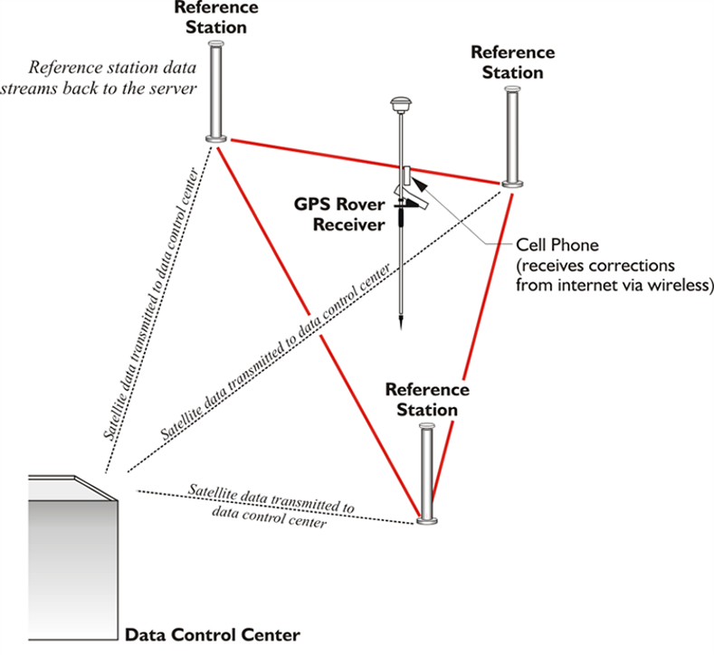
Real-TIme Network
Source: GPS for Land Surveyors
The pace of the development of Real-Time Networks, RTN, both by governments and commercial interests, is accelerating. The services are sometimes free and sometimes require the arrangement of a subscription or the payment of a fee before the user can access the broadcast corrections over a datalink via a modem such as a cell-phone or some other device. But the central idea at the foundation of RTN is differential correction. That is, the combination of observations from several CORS at known positions used to derive a model of an entire region still relies on the same differential ideas that we discussed near the beginning of the course. In other words, even the latest developments in satellite positioning continue to be based on the same fundamental principles.
In the next lesson, we will take a look at the changes in GPS/GNSS that will be affecting satellite positioning in the near future.
Before you go on to Lesson 9, double-check the Lesson 8 Checklist to make sure you have completed all of the activities listed there.
Lesson 9: GPS Modernization
The links below provide an outline of the material for this lesson. Be sure to carefully read through the entire lesson before returning to Canvas to submit your assignments.
Lesson 9 Overview
Overview
The configuration of the GPS Space Segment is well-known. A minimum of 24 GPS satellites ensure 24-hour worldwide coverage. But, today, there are more than that minimum on orbit. There are a few spares on hand in space. The redundancy is prudent. GPS, put in place with amazing speed considering the technological hurdles, is now critical to all sorts of positioning, navigation, and timing around the world. It’s that very criticality that requires the GPS modernization. The oldest satellites in the current constellation were launched in 1989. Imagine using a personal computer of that vintage today. It is not surprising that there are plans in place to alter the system substantially. What might be unexpected is many of those plans will be implemented entirely outside of the GPS system itself.
Objectives
At the successful completion of this lesson, students should be able to:
- recognize GPS Modernization;
- explain the difference between Block I, Block II, Block IIR, Block IIR-M, BLock IIF and Block III satellites;
- describe power spectral density diagrams;
- identify the M Code;
- define L2C;
- recognize L5;
Questions?
If you have any questions now or at any point during this week, please feel free to post them to the Lesson 9 Discussion Forum. (To access the forum, return to Canvas and navigate to the Lesson 9 Discussion Forum in the Lesson 9 module.) While you are there, feel free to post your own responses if you, too, are able to help out a classmate.
Checklist
Lesson 9 is one week in length. (See the Calendar in Canvas for specific due dates.) To finish this lesson, you must complete the activities listed below. You may find it useful to print this page out first so that you can follow along with the directions.
| Step | Activity | Access/Directions |
|---|---|---|
| 1 | Read the lesson Overview and Checklist. | You are in the Lesson 9 online content now. The Overview page is previous to this page, and you are on the Checklist page right now. |
| 2 | Read "Global Positioning System Modernization and Global Navigation Satellite Systems" pages 267 to 284 in Chapter 8 in GPS for Land Surveyors. | Text |
| 3 | Read the lecture material for this lesson. | You are currently on the Checklist page. Click on the links at the bottom of the page to continue to the next page, to return to the previous page, or to go to the top of the lesson. You can also navigate the lecture material via the links in the Lessons menu. |
| 4 | Participate in the Discussion. | To participate in the discussion, please go to the Lesson 9 Discussion Forum in Canvas. (That forum can be accessed at any time by going to the GEOG 862 course in Canvas and then looking inside the Lesson 9 module.) |
| 5 | Read lesson Summary. | You are in the Lesson 9 online content now. Click on the "Next Page" link to access the Summary. |
GPS Modernization

The configuration of the GPS Space Segment is well known. The satellites are on orbit at a nominal height of about 20,000 km above the Earth. There are three carriers L1 (1575.42 MHz), L2 (1227.60 MHz), and L5 (1176.42 MHz). A minimum of 24 GPS satellites ensure 24-hour worldwide coverage, but there are more than that minimum on orbit. There are a few spares on hand in space. The redundancy is prudent because GPS is critical to positioning, navigation and timing. It is also critical to the smooth functioning of financial transactions, air traffic, ATMs, cell phones, and modern life in general around the world. This very criticality requires continuous modernization.
GPS was put in place with amazing speed considering the technological hurdles and reached its Fully Operational Capability (FOC) on July 17, 1995. The oldest satellites in the current constellation were launched in the late 1990s. If you imagine using a personal computer of that vintage today, it is not surprising that there are plans in place to alter the system substantially. In 2000, U.S. Congress authorized the GPS III effort. The project involves new ground stations and satellites, additional civilian and military navigation signals, and improved availability. This chapter is about some of the changes in the modernized GPS, its inclusion in the Global Navigation Satellite System and more. Block I GPS SatelliteBlocks I and II GPS Satellitesthe design life has obviously been exceeded in most cases, Block IIA satellites do wear out. Block IIR GPS Satellite.
Satellite Blocks
Block I

| Demonstrated GPS |
|---|
|
The 11 GPS satellites launched from Vandenberg Air Force Base between 1978 and 1985 were known as Block I satellites. The last Block I satellite was retired in late 1995. Ten of the satellites built by Rockwell International achieved orbit on Atlas F rockets. There was one launch failure. All were prototype satellites built to validate the concept of GPS positioning. This test constellation of Block I satellites was inclined by 63° to the equator instead of the current specification of 55°. They could be maneuvered by hydrazine thrusters operated by the control stations.
The first GPS satellite was launched February 22, 1978 and was known as Navstar 1. An unfortunate complication is that this satellite was also known as PRN 4 just as Navstar 2 was known as PRN 7. The Navstar number, or Mission number includes the Block name and the order of launch, for example I-1, meaning the first satellite of Block I. and the PRN number refers to the weekly segment of the P code that has been assigned to the satellite, and there are still more identifiers. Each GPS satellite has a Space Vehicle number, an Interrange Operation Number, a NASA catalog number, and an orbital position number as well. However, in most literature, and to the GPS receivers themselves, the PRN number is the most important.
Continuing the discussion of the space segment, here is the Block 1 satellite. These were the first launched. There are none of them functional today. But they certainly did an extraordinary job in getting the system started. It was an experimental system at that time. But it certainly has worked out well.
The Block I satellites weigh 845 kg in final orbit. They were powered by three rechargeable nickel-cadmium batteries and 7.25 square meters of single-degree solar panels. These experimental satellites served to point the way for some of the improvements found in subsequent generations. For example, even with the back-up systems of rubidium and cesium oscillators onboard each satellite, the clocks proved to be the weakest components. The satellites, themselves, could only store sufficient information for 3½ days of independent operation. And the uploads from the control segment were not secure; they were not encrypted. Still, all 11 achieved orbit, except Navstar 7. The design life for these satellites was 4½ years, but their actual average lifetime was 8.76 years. That is something that continues. The GPS satellites have mostly outlived their design life. There are no Block I satellites operating today.
Block II

| Some of the iMprovements over Block I |
|---|
|
The next generation of GPS satellites are known as Block II satellites. The first left Cape Canaveral on February 14, 1989, almost 14 years after the first GPS satellite was launched. It was about twice as heavy as the first Block I satellite and was expected to have a design life of 7½ years with a Mean Mission Duration, MMD of 6 years. The Block II satellites could operate up to 14 days without an upload from the control segment and their uploads were encrypted. The satellites themselves were radiation hardened, and their signals were subject to selective availability.
These satellites were built by Rockwell International. Block II included the launch of 9 satellites between 1989 and 1990. None of the Block II satellites are in the constellation today. the last was decommissioned in 2007
Block IIA

| Some of the iMprovements over Block II |
|---|
|
The launch of the Block IIA satellites began in 1990. 19 Block IIA satellites, with several navigational improvements, were launched between 1990 and 1997. Block IIA satellites could store more of the Navigation message than the Block II satellites, and could, therefore, operate without contact with the Control Segment for 6 months. However, if that were actually done, their broadcast ephemeris and clock correction would have degraded. None of the Block IIA satellites are in the constellation today.
Block IIR

| Some of the iMprovements over Block IIA |
|---|
|
The first launch of the next Block, Block IIR satellites in January of 1997 was unsuccessful. The following launch in July of 1997 succeeded. The third generation of GPS satellites is known as Block IIR satellites, the R stands for replenishment. There are two significant advancements in these satellites. The Block IIR satellites have enhanced autonomous navigation capability because of their use of intersatellite linkage (called AutoNav). This involves their use of reprogrammable processors onboard to do their own fixes in flight. There are Block IIR satellites in the constellation today.
Block IIR-M

| Some of the iMprovements over Block IIR |
|---|
|
In September of 2005, the first of the next improved block, called Block IIR-M was launched. These are IIR satellites that were modified before they were launched. The modifications upgraded these satellites so that they radiate two new codes; a new military code, the M code, a new civilian code, the L2C code, and demonstrate a new carrier, L5. There are Block IIR-M satellites in the constellation today.
Block IIF

| Some of the iMprovements over Block IIR-M |
|---|
|
The L2C signal and the third civilian carrier will be very helpful because, as you know, ionosphere modeling is an important part of error management in GPS. We can model it to some good degree with two carriers. Three will obviously make that modeling even better.
Block IIF is the most recent group of GPS satellites launched and the first of them reached orbit in May of 2010. There has been steady and continuous improvement in the GPS satellite constellation from the beginning.
The first Block IIF satellite was launched in the summer of 2010. Their design life is 12 to 15 years. Block IIF satellites have faster processors and more memory onboard. They broadcast all of the previously mentioned signals including the L5 carrier, This signal was demonstrated on the Block IIR-M and is available from all of the Block IIF satellites. The Block IIF satellites replaced the Block IIA satellites as they aged. Their onboard navigation data units (NDU) support the creation of new navigation messages with improved broadcast ephemeris and clock corrections. Like the Block IIR satellites, the Block IIF can be reprogrammed on orbit.
Block III
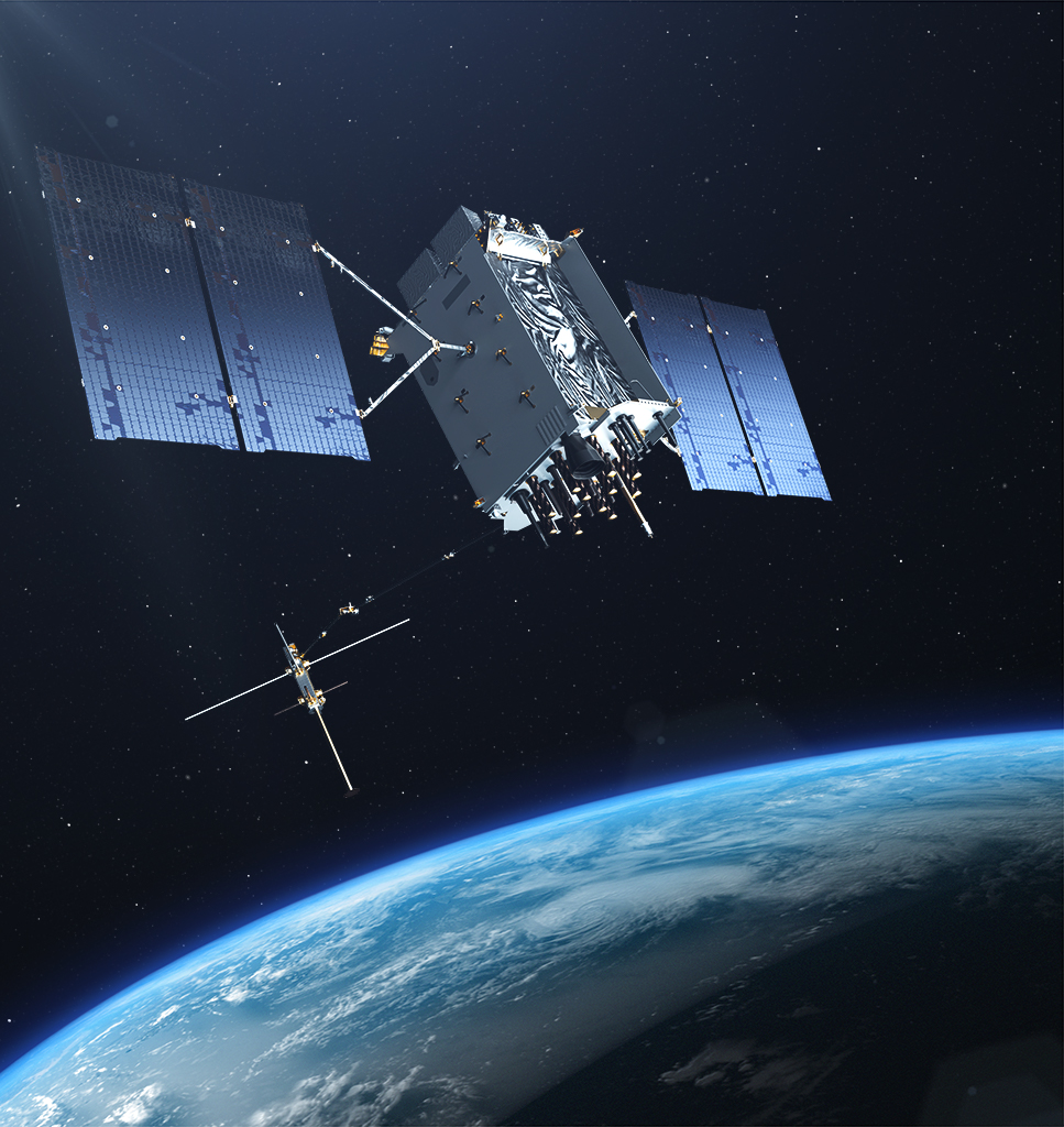
| Some of the iMprovements over Block IIF |
|---|
|

The Legacy Signals and Power Spectral Density Diagrams
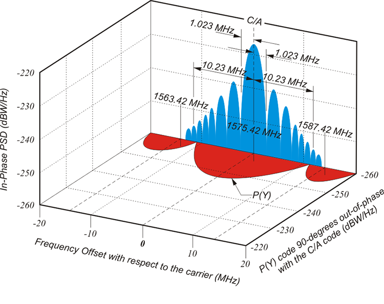
The Power Spectral Density (PSD) diagrams show the increase or decrease, in decibels, of power in Watts with respect to frequency in Hertz. It allows you to see some of the things we've already discussed. For example, this is the C/A Code in the blue on the L1 carrier, which, of course, is centered at 1,575.42 megahertz and then spread over a bandwidth that is spread spectrum. It's about 10.23 megahertz on each side for a total of like 20.46. That in the red, you see the P(Y) Code is in quadrature 90 degrees from the C/A Code. It has really one main lobe and then two sidebands, and then the blue C/A Code has many lobes.

The L2 signal diagram is centered on 1,227.60 MHz. As you can see, it is similar to the L1 diagram except for the absence of the C/A code which is, of course, not carried on the L2 frequency. As well-known as these are, this state of affairs is changing.
Power Spectral Density Diagrams
Many of the improvements in GPS are centered on the broadcast of new signals. Therefore, it is pertinent to have a convenient way to visualize all the GPS and GNSS signals that illustrate the differences in the new signals and a good deal of signal theory as well. It is a diagram of the power spectral density function (PSD). They graphically illustrate the signal's power per bandwidth in Watts per Hertz as a function of frequency. In GPS and GNSS literature, the PSD diagram is often represented with the frequency in MHz on the horizontal axis and the density, the power, represented on the perpendicular axes in decibels relative to one Hertz per Watt or dBW/Hz.
The actual definition of PSD is the Fourier transform of the autocorrelation function, but the idea behind them is to give you an idea of the power within a signal with regard to frequency. These graphics show the increase or decrease, in decibels, of power, in Watts with respect to frequency in Hertz, of the well-known signals on L1 and L2.
dBW/Hz
Perhaps a bit of background is in order to explain those units. A bel unit originated at Bell Labs to quantify power loss on telephone lines. A decibel is a tenth of a bel. A decibel, dB, is a dimensionless number. In other words, it's a ratio that can acquire dimension by being associated with measured units. A change of 1 decibel would be an increase or a decrease of 27 percent. A change of 3 decibels would be an increase or a decrease of 100 percent. Here are some of the quantities with which it is sometimes associated: seconds of time, symbolized dBs, bandwidth measured in Hertz, symbolized dBHz, and temperature measured in Kelvins, symbolized dBK. Since signal power is of interest here, dB will be described with respect to 1Watt, the symbol used is dBW.
dBW is a short, concise number that can conveniently express the wide variation in GPS signal power levels. dBW can represent quite large and quite small amounts of power more handily than other notations. For example, consider a value of interest in GPS signals. The value is very small, one tenth of a millionth billionth of a watt. Expressing it as 0.0000000000000001 W is a bit exhausting. It would be more convenient expressed in dBW, a value that can be derived using the formula.
where is the power of the signal.
The expression -160 dBW is immediately useful. Here's an example. A change in 3 decibels is always an increase or a decrease of 100% in power level. Stated another way, a 3-decibel increase indicates a doubling of signal strength and a 3-decibel decrease indicates a halving of signal strength. Therefore, it is easy to see that a signal of -163 dBW has half the power of a signal of -160dBW. Considering the broadcasts from the current constellation of satellites, the minimum power received from the P code on L1 by a GPS receiver on the Earth's surface is about -163 dBW, and the minimum power received from the C/A code on L1 is about -160dBW. This difference between the two received signals is not surprising, since at the start of their trip to Earth they are transmitted by the satellite at power levels that are also 3 decibels apart. The P code on L1is transmitted at a nominal +23.8 dBW (240 W), whereas the nominal transmitted power of the C/A code on L1 is +26.8 dBW (479 W). It is interesting to note that the minimum received power of the P code on L2 is even less at -166 dBW, and its nominal transmitted power is +19.7 dBW (93 W).
One might wonder why there are such differences between the power of the transmitted GPS signal, called the Effective Isotropic Radiated Power (EIRP), and the power of the received signal. The difference is large. It is 186 to 187 dB, nearly 10 quintillion decibels. The loss is mostly because is the 20,000 km distance from the satellite to a GPS receiver on the Earth. There is also an atmospheric loss and a polarization mismatch loss, but the biggest loss by far, about 184 dB, is along the path in free space.

Much of this loss is a function of the spreading out of the GPS signal in space, as described by the inverse square law. The intensity of the GPS signal varies inversely to the square of the distance from the satellite. In other words, by the time the signal makes that trip and reaches the GPS receiver, it is pretty weak, as shown in the 'Inverse Square Law' figure above (Figure 8.3 from the textbook). It follows that GPS signals are easily degraded by vegetation canopy, urban canyons, and other interference.
A GPS signal has power, of course, but it also has bandwidth. PSD is a measure of how much power a modulated carrier contains within a specified bandwidth. That value can be calculated using the following formula and allowing that there is an even distribution of 10-16 W over the 2.046 MHz C/A bandwidth of the C/A code:
The calculation is also frequently normalized and done presuming an even distribution of 1W over the 2.046 MHz C/A bandwidth of the C/A code. In other words, the following calculation presumes an even distribution of the power over 1W instead of the 10-16 W used in the previous calculation:
The M-Code

New Signals
An important aspect of GPS modernization is the advent of some new and different signals that are augmenting the old reliable codes. In GPS, a dramatic step was taken in this direction on September 21, 2005 when the first Block IIR-M satellite was launched. One of the significant improvements coming with the Block IIRM satellites is increased L-band power on both L1 and L2 by virtue of the new antenna panel. The Block IIR-M satellites will also broadcast new signals, such as the M-code.

The M-Code
Eight to twelve of these replenishment satellites are going to be modified to broadcast a new military code, the M-code. This code will be carried on both L1 and L2 and will probably replace the P(Y) code eventually. It has the advantage of allowing the Department of Defense (DoD) to increase the power of the code to prevent jamming. There was consideration given to raising the power of the P(Y) code to accomplish the same end, but that strategy was discarded when it was shown to interfere with the C/A code.
The M-code was designed to share the same bands with existing signals, on both L1 and L2, and still be separate from them. See those two peaks in the M-code in the illustration. They represent a split-spectrum signal about the carrier. Among other things, this allows minimum overlap with the maximum power densities of the P(Y) code and the C/A code, which occur near the center frequency. That is because the actual modulation of the M-code is done differently. It is accomplished with binary offset carrier (BOC) modulation, which differs from the binary phase shift key (BPSK) used with the legacy C/A and P(Y) signals. As a result of this BOC modulation, the M-code has its greatest power density at the edges, which is at the nulls, of the L1 away from P(Y) and C/A. This architecture both simplifies implementation at the satellites and receivers and also mitigates interference with the existing codes. Suffice it to say that this aspect and others of the BOC modulation strategy offer even better spectral separation between the M-code and the older legacy signals.
The M-code is unusual in that a military receiver can determine its position with the M-code alone, whereas with the P(Y) it must first acquire the C/A code to do so. It is also spread across 24 MHz of the bandwidth.
Perhaps it would also be useful here to mention the notation used to describe the particular implementations of the Binary Offset Carrier. It is characteristic for it to be written BOC (α, ß). Here the α indicates the frequency of the square wave modulation of the carrier, also known as the subcarrier frequency factor. The ß describes the frequency of the pseudorandom noise modulation, also known as the spreading code factor. In the case of the M-code, the notation BOC (10, 5) describes the modulation of the signal. Both here are multiples of 1.023 MHz. In other words, their actual values are.
.
The M-code is tracked by direct acquisition. This means that, as mentioned in Lesson 1, the receiver correlates the signal coming in from the satellite with a replica of the code that it has generated itself.
One of the significant improvements coming from the Block IIR-M satellites is increased L band power on both L1 and L2. This new M-Code will possibly replace the P-Code, eventually. It will be carried on both L1 and L2, and it has an advantage that the Department of Defense can increase the power of the code to prevent jamming. There was consideration to raising the power of the Y-Code to accomplish the same end, but that was discarded when it was shown to interfere with the C/A Code. So to recap, the M-Code will be carried on L1 and L2, but because of the binaries offset carrier modulation, it will not interfere with the older legacy codes, the C/A Code and P-Code.
L2C and CNAV

L2 Signal
In the illustration, the L2 signal diagram is centered on 1227.60 MHz. As you can see, it is similar to the L1 diagram except for the absence of the C/A code, which is, of course, not carried on the L2 frequency. As well-known as these are, this state of affairs is changing. We have been using the L2 carrier since the beginning of GPS, of course, but there will be two new codes broadcast on the carrier, L2, that previously only carried one military signal exclusively, the P(Y) code. L2 will carry a new military signal, the M-code, just discussed, and a new civil signal as well.
On the upper portion of this diagram, you see the L2 carrier, of course, with only the P-Code encrypted as the Y-Code. In the lower part, there is the same L2 with P-Code, but the M-Code is included, and there's a new civilian code. This one is called L2C. Before this, there was no civilian code on L2. There was only the C/A Code on L1. However, these new IIR-M satellites will be carrying the L2C, a civil code on L2. We've been using the L2 carrier since the beginning of GPS, of course, but there will be two new codes broadcast on that carrier, the M-Code and the new Civilian code L2C.
L2C
A new military code on L1 and L2 may not be terribly exciting to civilian users, but these IIR-M satellites have something else going for them. They broadcast a new civilian code. We have been using the L2 carrier since the beginning of GPS of course, but there will be two new codes broadcast on the carrier, L2, that previously only carried one military signal, the P(Y) code. L2 will carry the new military signal, the M-code, and a new civil signal as well. This is a code that was first announced back in March of 1998. It is transmitted by all block IIR-M satellites and subsequent blocks and is known as L2C. The “C” is for civil.
Even though its 2.046 MHz from null-to-null gives it a very similar power spectrum to the C/A code, it is important to note that L2C is not a copy of the C/A-code even though that was the original idea. The original plan was that it would be a replication of the venerable C/A code, but carried on L2 instead of L1. This concept changed when Colonel Douglas L. Loverro, Program Director for the GPS Joint Program Office (JPO), was asked if perhaps it was time for some improvement of C/A. The answer was yes. The C/A code is somewhat susceptible to both waveform distortion and narrow-band interference, and its cross-correlation properties are marginal at best. So, the new code on L2, known as L2 civil, or L2C was announced. It is more sophisticated than C/A. So, the L2C is actually a different code than the C/A. Still, it's a civilian accessible code, and it's carried on L2 instead of L1.
Civil-Moderate (CM) and Civil-Long (CL)
L2C is actually composed of two pseudorandom noise signals: the civil-moderate length code, CM, and the civil long code, CL. They both utilize the same modulation scheme, binary phase shift key (BPSK), as the legacy signals, and both signals are broadcast at 511.5 kilobits per second (Kbps). This means that CM repeats its 10230 chips every 20 milliseconds, and CL repeats its 767250 chips every 1.5 seconds. But, wait a minute, how can you do that? How can you have two codes in one?

L2C achieves this by time multiplexing. Since the two codes have different lengths L2C alternates between chips of the CM code and chips of the CL code as shown in the illustration. It is called chip-by-chip time multiplexing. So, even though the actual chipping rate is 511.5 KHz, half the chipping rate of the C/A code, with the time multiplexing it still works out that taken together L2C ends up having the same overall chip rate as L1 C/A code, 1.023 MHz . This provides separation from the M code.
In this illustration, I try to answer the question how it's possible in L2C to have two codes, the CM Code and the CL Code, simultaneously operating on the same signal. It's known as multiplexing, and we discussed that briefly when we were talking about receivers, except, in this case, it's chip by chip time multiplexing. The CM Code, the moderate length code, goes through 10,238 chips before it repeats. It repeats every 20 milliseconds, but the CL Code, the long code, repeats after 1.5 seconds.
Those lengths give you very good cross correlation protection. In fact, both are longer than the C/A Code and present a subsequent improvement in autocorrelation. This is because the longer the code, the easier it is to keep the desired signal separate from the background. In practice, this means that these signals can be acquired with more certainty by a receiver which can maintain locking them more surely in marginal situations where the sky is obstructed.
So, it is possible to have these two signals, the CM and the CL on the L2C because the receiver can shift back and forth between the two with good, solid cross correlation and lock on to the signals even in circumstances where the sky is obstructed better than one can with the C/A Code. It's important to note that the L2C is actually slightly weaker, 2.3 decibels weaker, than the C/A Code. And it's surprising that this is not a disadvantage, because the receiver can track the long dataless CL, that's the long code on L2C with the phase locked loop instead of squaring Costas loop.
In other words, the long dataless sequence of the CL provides for correlation that is actually about 250 times stronger than the C/A Code. So, despite the fact that its transmission power is 2.3 decibels weaker compared to the C/A Code, the L2C has 2.7 decibels greater data recovery and 0.7 decibels greater carrier tracking. It's actually more solid, even though the power is slightly less.
L2C has better autocorrelation and cross-correlation protection than the C/A code because both of the CM and CL codes are longer than the C/A code. Longer codes are easier to keep separate from the background noise. In practice, this means these signals can be acquired with more certainty by a receiver that can maintain lock on them more surely in marginal situations where the sky is obstructed.
There is also another characteristic of L2C that pays dividends when the signal is weak. While CM carries newly formatted navigation data and is, therefore, known as the data channel, CL does not. It is dataless and known as a pilot channel. A pilot channel can support longer integration when the signal received from the satellite is weak. This is an idea that harks all the way back to Project 621B at the very beginnings of GPS. The benefits of a pilot channel distinct from the data components carried by a signal was known in the 1960s and 1970s but was not implemented in GPS until recently.
Phase-Locked Loop
Even though the L2C signals’ transmission power is 2.3 dB weaker than is C/A on L1, and even though it is subject to more ionospheric delay than the L1 signal, L2C is still much more user friendly. The long data-less CL pilot signal has 250 times (24dB) better correlation protection than C/A. This is due in large part to the fact that the receiver can track the long data-less CL with a phase-locked loop instead of a squaring Costas loop that is necessary to maintain lock on CM, C/A and P(Y). This allows for improved tracking from what is, in fact, a weaker signal and a subsequent improvement in protection against continuous wave interference. As a way to illustrate how this would work in practice, here is one normal sequence by which a receiver would lock onto L2C. First, there would be acquisition of the CM code with a frequency locked or Costas loop, next there would be testing of the 75 possible phases of CL, and finally acquisition of CL. The CL, as mentioned, can be then tracked with a basic phase-locked loop. Using this strategy, even though L2C is weaker than C/A there is actually an improvement in the threshold of nearly 6 dB by tracking the CL with the phase-locked loop. Compared to the C/A code L2C has 2.7 dB greater data recovery and 0.7 dB greater carrier-tracking.
Practical Advantages
Great, so what does all that mean in English? Having two civilian frequencies being transmitted from one satellite affords the ability to model and lessen the ionospheric delay error for that satellite while relying on code phase pseudorange measurements alone. In the past, ionospheric modeling was only available to multi carrier frequency observations, or by reliance on the atmospheric correction in the Navigation message. Before May 2, 2000 with Selective Availability on a code-based receiver could get you within 30 to 100 meters of your true position; when SA was turned off, that was whittled down to 15 to 20 meters or so under very good conditions. But with just one civilian code C/A on L1, there was no way to remove the second largest source of error in that position, the ionospheric delay.

But with two civilian signals, one on L1 (C/A) and one on L2 (L2C), it becomes possible to effectively model the ionosphere using code phase. In other words, it may become possible for an autonomous code-phase receiver to achieve positions with a 5-10m positional accuracy with some consistency.
The L2C signal also ameliorates the effect of local interference. This increased stability means improved tracking in obstructed areas like woods, near buildings, and urban canyons. It also means fewer cycle slips.

With L2C, there will be a better tolerance for interference, increased stability, and fewer cycle slips. That means that GPS will work better in obstructed areas, and this will be a practical advantage to those like the fellow with his receiver looking up to an obstructed sky. A second civilian code on a separate frequency is another really practical advantage. You can model the ionosphere with a multi-frequency receiver because of the dispersive characteristic of the ionosphere. However, those that have been operating purely in code phase or pseudo range positions have not had that advantage. Now, with L2C on L2, and C/A Code on L1, there will be two civilian accessible codes available to a code phase pseudo range receiver making it possible to model the ionosphere with a code observation. This should improve the positions available from purely code phase receivers quite a bit.
So, even if it is the carrier-phase that ultimately delivers the wonderful positional accuracy we all depend on, the codes get us in the game and keep us out of trouble every time we turn on the receiver. The codes have helped us to lock on to the first satellite in a session and allowed us to get the advantage of cross-correlation techniques almost since the beginning of GPS. In other words, our receivers have been combining pseudorange and carrier-phase observables in innovative ways for some time to measure the ionospheric delay, detect multipath, do wide laning, and so forth. But those techniques can be improved, because while the current methods work, the results can be noisy and not quite as stable as they might be, especially over long baselines. It will be cleaner to get the signal directly once there are two clear civilian codes, one on each carrier. It may also help reduce the complexity of the chipsets inside our receivers, and might just reduce their cost as well.
Along that line, it is worthwhile to recall that the L2C has an overall chip rate of 1.023 MHz, just like L1 C/A. Such a slow chip rate can seem to be a drawback until you consider that that rate affects the GPS chipset power consumption. In general, the slower the rate, the longer the battery life, and the improvement in receiver battery life could be very helpful. And not only that, the slower the chip rate, the smaller the chipset. That could mean more miniaturization of receiver components.
L2C is clearly going to be good for the GPS consumer market, but it also holds promise for surveyors. Nevertheless, there are a few obstacles to full utilization of the L2C signal. It will be some time before the constellation of Block IIR-M necessary to provide L2C at an operational level is up and functioning. Additionally, aviation authorities do not support L2C. It is not in an Aeronautical Radionavigation Service (ARNS) protected band. It happens that L2 itself occupies a radiolocation band that includes ground-based radars.

Click here to see a text description.
| Messages (pseudo-packetized) | 1 Word | 2 Words | 3-10 Words |
|---|---|---|---|
| 0 | MT | How | Default |
| 10 | MT | How | Ephemeris 1 |
| 11 | MT | How | Ephemeris 2 |
| 13 | MT | How | Clock Differential Correction |
| 14 | MT | How | Ephermis Differential Correction |
| 15 | MT | How | Text |
| 30 | MT | How | Clock, IONO, &Group Delay |
| 31 | MT | How | Clock & Reduced Almanac |
| 63 | MT | How | MT7-67 still to be defined |
CNAV
The navigation data on CM portion of the L2C signal is improved over the legacy Navigation message. It is called CNAV. It was tested using some of the message types, MT, shown in the illustration in June of 2013.
You may recall that the legacy Navigation message was mentioned in Chapter 1. It is also known by the acronym NAV. The information in CNAV is fundamentally the same as that in the original NAV message, but there are differences. It includes the almanac, ephemerides, time, and satellite health. CNAV contains 300-bit messages like the legacy NAV message, but CNAV packages its 12-second, 300-bit messages differently. Instead of the repetition of frames and sub-frames in a fixed pattern as is the case with the legacy NAV, CNAV utilizes a pseudo-packetized message protocol. One of every four of these packets includes clock data; two of every four contains ephemeris data, and so on. This makes CNAV more flexible than NAV. The order and the repetition of the individual messages in CNAV can be varied. CNAV can accommodate the transmission of the information in support of 32 satellites using 75% or less of its bandwidth. CNAV is also more compact than NAV, and that allows a receiver to get to its first fix on a satellite much faster.
A packet in message 35 of CNAV was assigned to the time offset between GPS and GNSS in the June 2013 test. Such a message would be a boon for interoperability between GPS, Galileo, and GLONASS. Also, each packet contains a flag which can be toggled on within a few seconds of the moment a satellite is known to be unhealthy. This is exactly the sort of quick access to information necessary to support safety-of-life applications. Only a fraction of the available packet types are being used at this point. CNAV is designed to grow, and can accommodate 63 satellites as the system requires. For example, there could be packets that would contain differential correction like that available from satellite-based augmentation systems (SBAS).
There is also a very interesting aspect to the data broadcast on CM known as Forward Error Correction (FEC). An illustration of this technique is to imagine that every individual piece of data is sent to the receiver twice. If the receiver knows the details of the protocol to which the data ought to conform, it can compare each of the two instances it has received to that protocol. If they both conform, there is no problem. If one does and one does not, the piece of data that conforms to the protocol is accepted and the other is rejected. If neither conforms, then both are rejected. Using FEC allows the receiver to correct transmission errors itself, on the fly. FEC will ameliorate transmission errors and reduce the time needed to collect the data.
There is a packet in CNAV that may be assigned to the time offset between GPS and GNSS. So, one of the things we'll talk about is that GLONASS's time standard is different than that of GPS, and the difference can be loaded into the navigation message, so there's some preparation here for the GNSS future. Each packet contains a flag that can be turned on and off very quickly to indicate that a satellite is unhealthy. This could be quite useful for safety of life, things such as ambulances and so on. Because if a satellite should not be used in positioning if it will corrupt the results, it's important to know that immediately in real time. It's great to have a system that can provide that.
L5

Alright, L2C is fine, but what about L5, the new carrier being broadcast on the Block IIF satellites? It is centered on 1176.45 MHz, 115 times the fundamental clock rate.
As you see from the illustration, the basic structure of L5 looks similar to that of L1. There are two pseudorandom noise (PRN) codes on this 20 MHz carrier. The two codes are modulated using Quad Phase Shift Key (QPSK), and they are broadcast in quadrature to each other. However, borrowing a few pages from other recent developments, the in-phase (I) signal carries a data message that is virtually identical to the CNAV on L2. The other, the quadraphase signal (Q), is data-less and L5 utilizes chip-by-chip time multiplexing in broadcasting its two codes, as does L2C in broadcasting CM and CL.
Both L5 codes have a 10.23 MHz chipping rate, the same as the fundamental clock rate. This is the same rate that has been available on the P(Y) code from the beginning of the system. However, this is the fastest chipping rate available in any civilian code. L5 has the only civilian codes that are both ten times longer and ten times faster than the C/A code. Since the maximum resolution available in a pseudorange is typically about 1% of the chipping rate of the code used, the faster the chipping rate, the better the resolution.
L5 has about twice as much power as L1, and since L5 does not carry military signals, it achieves an equal power split between its two signals. In this way, L5 lowers the risk of interference and improves multipath protection. It also makes the data-less signal easier to acquire in unfavorable and obstructed conditions.
Unlike L2C, L5 users will benefit from its place in a band designated by the International Telecommunication Union (ITU) for the Aeronautical Radionavigation Navigation Services (ARNS) worldwide. Therefore, it is not prone to interference with ground based navigation aids and is available for aviation applications. While no other GPS signal occupies this band, L5 does share space with one of the Galileo signals, E5. L5 does also incorporate Forward Error Correction (FEC).
It is helpful that L5 will share space with one of the E5A signal from an entirely separate satellite system, Galileo. This is the European contribution to GNSS. The fast chipping rate on L5 is also good news.
Block IIF and Block III

The first Block IIF satellite was launched in the summer of 2010. As of 2014. There are 12 Block IIF satellites on orbit. Their design life is 12 to 15 years. Block IIF satellites have faster processors and more memory onboard. They broadcast all of the previously mentioned signals, and one more, a new carrier known as L5. This is the signal that was demonstrated on the Block IIR-M. It is available from all of the Block IIF satellites. The L5 signal is within the Aeronautical Radio Navigation Services (ARNS) frequency and can service aeronautical applications. The improved rubidium frequency standards on Block IIF satellites have a reduced white noise level. The Block IIF satellite's launch vehicles can place the satellites directly into their intended orbits, so they do not need the apogee kick motors their predecessors required. All of the Block IIF satellites will carry DASS repeaters. Their onboard navigation data units (NDU) support the creation of new navigation messages with improved broadcast ephemeris and clock corrections. The Block IIF can be reprogrammed on orbit.

Block III satellite
There are currently 3 Block IIIA satellites on orbit and operational. They broadcast all of the previously mentioned signals and one more, L1C.
Summary of C/A, L2C, and L5

GPS modernization is underway. New spacecraft with better electronics, better navigation messages, newer and better clocks are just part of the story. Beginning with the launch of the first IIR-M satellite, new civil signals began to appear, starting with L2C which was followed by L5 on the Block IIF satellites.
These signals tend to have longer codes, faster chipping rates, and more power than the C/A and P(Y) codes have. In practical terms, these developments lead to faster first acquisition, better separation between codes, reduced multipath and better cross-correlation properties.
The legacy L1 and L2 signals are at the top of the illustration. In the next tier, you see the L1 with the addition of the M-Code and substantially the same otherwise. L2 has both the M-Code and the new L2C Civilian code. In the third tier and the Block IIF satellites, there is the addition of L5.
New Signal Availability and Some Benefits
| Carrier | Signal | Block IIR | Block IIR-M | Block IIF |
|---|---|---|---|---|
| L1 | P/Y | ⦿ | ⦿ | ⦿ |
| L2 | P/Y | ⦿ | ⦿ | ⦿ |
| L1 | CA | ⦿ | ⦿ | ⦿ |
| L2 | L2C | ⦿ | ⦿ | |
| L1 | M | ⦿ | ⦿ | |
| L2 | M | ⦿ | ⦿ | |
| L5 | Civil | ⦿ |
In the table, you see that the Block IIR-M satellites have the addition of the M-Code and the L2C to the legacy signals available from the Block IIR satellites. The Block IIF satellites IIFs have all the previous codes and L5.
Ionospheric Bias
Concerning the effect of the ionosphere—as you know, ionospheric delay is inversely proportional to frequency of the signal squared. So it is that L2’s atmospheric bias is about 65% larger than L1, and it follows that the bias for L5 is the worst of the three at 79% larger than L1. L1 exhibits the least delay, as it has the highest frequency of the three.
Correlation Protection
Where a receiver is in an environment where it collects some satellite signals that are quite strong and others that are weak, such as inside buildings or places where the sky is obstructed, correlation protection is vital. The slow chipping rate, short code length, and low power of L1 C/A means it has the lowest correlation protection of the three frequencies L1, L2, and L5. That means that a strong signal from one satellite can cross correlate with the codes a receiver uses to track other satellites. In other words, the strong signal will actually block collection of the weak signals. To avoid this, the receiver is forced to test every single signal so to avoid incorrectly tracking the strong signal it does not want instead of a weak signal that it does. This problem is much reduced with L2. It has a longer code length and higher power than L1. It is also reduced with L5 as compared to L1. L5 has a longer code length, much higher power, and a much faster chipping rate than L1. In short, both of the civilian codes on L2 and L5 have much better cross correlation protection and better narrowband interference protection than L1, but L5 is best of them all.
L1C

L1C Another Civil Signal
Another civil signal is broadcast by the Block III satellites. It is known as L1C. As a result of an agreement between the United States and the European Union (EU) reached in June 2004, this signal will be broadcast by both GPS and Galileo’s L1 Open Service signals. It will also be broadcast by the Japanese Quasi-Zenith Satellite System (QZSS), the Indian Regional Navigation Satellite System (IRNSS), and China's BeiDou system. These developments open extraordinary possibilities of improved accuracy and efficiency when one considers there may eventually be a combined constellation of 50 or more satellites, all broadcasting this same civilian signal. All this is made possible by the fact that each of these different satellite systems utilizes carrier frequencies centered on the L1, 1575.42 MHz. Perhaps that has something to do with the fact that L1, having the highest frequency, experiences the least ionospheric delay of the carrier frequencies. There are many signals on L1, but looking at GPS alone, there is the C/A code, the P(Y) code, the M code and now L1C code. It is a challenge to introduce yet another code on the crowded L1 frequency and still maintain separability.
As shown in the figure above, the L1C design shares some of the M code characteristics, i.e., Binary Offset Carrier. It has some similarities with L2C. For example, it has a data-less pilot signal (L1CP) and a signal with a data message (L1CD) whose codes are of the same length as CM on L2C 10,230 chips and broadcast at 1.023 Mbps. The data signal uses BOC (1, 1) modulation, and the pilot uses time multiplexed binary offset carrier (TMBOC). The TMBOC is BOC (1, 1) for 29 of its 33 cycles, but switches to BOC (6, 1) for 4 of them. The pilot component has 75% of the signal power, and the data portion of the signal has 25%. This means that L1C has good separation from the other signals on L1, a good tracking threshold, and a receiver reaches its first fix to the satellite broadcasting L1C faster. The utility of L1C is further enhanced by the fact that it has double, 1.5dB, the power of C/A.
The message carried by L1CD is known as CNAV-2. Unlike CNAV, CNAV-2 has frames. Each frame is divided into three sub-frames. Both CNAV and CNAV-2 have 18% more satellite ephemeris information than NAV. The structure of CNAV-2 virtually ensures that once a receiver acquires the satellite, the time to first fix will not exceed 18 seconds.
L1C will likely be operational in a few years. However, it will not be fully operational until it is broadcast by 24 satellites
Discussion
Discussion Instructions
To continue the discussion begun by this lesson, I would like to pose this question:
What are some of the practical applications of GPS that may be enhanced by the systems modernization? What effects do you foresee on everyday applications? Do you think typical smart phones will be capable of realizing such benefits for the user? Why? or why not?
To participate in the discussion, please go to the Lesson 9 Discussion Forum in Canvas. (That forum can be accessed at any time by going to the GEOG 862 course in Canvas and then looking inside the Lesson 9 module.)
Summary
GPS modernization is underway. New spacecraft with better electronics, better navigation messages, newer and better clocks are just part of the story. That’s great, but does all that mean to you? Please give your impression of the practical applications that might be affected by these changes in the discussion forum. What do you think?
In the next lesson, we will look ahead at GNSS and try to do a bit of forecasting about what new constellations and new signals might bring us.
Before you go on to Lesson 10, double-check the Lesson 9 Checklist to make sure you have completed all of the activities listed there.
Lesson 10: Global Navigation Satellite Systems and the Future
The links below provide an outline of the material for this lesson. Be sure to carefully read through the entire lesson before returning to Canvas to submit your assignments.
Lesson 10 Overview
Overview
The GPS system is one component of the worldwide effort now known as the Global Navigation Satellite System, GNSS. Another component of GNSS is the GLONASS system of the Russian Federation, a third is the GALILEO system administered by the EU and a fourth is the Chinese Beidou system. The concept is the use of these networks of satellites and others together. Further, they will be augmented by both ground-based augmentation systems, GBAS, and space-based augmentation systems, SBAS, to provide positioning, navigation, and timing solutions to users around the world. One goal of this cooperation is interoperability. Interoperability is the idea that properly equipped receivers will be able to obtain useful signals from all available satellites in all the constellations and have their solutions improved rather than impeded by the various configurations of the different satellite broadcasts.
Objectives
At the successful completion of this lesson, students should be able to:
- recognize the benefits of L1C;
- define BPSK modulation scheme;
- define BOC modulation scheme;
- explain the difference between BPSK and BOC modulation schemes;
- define the GLONASS FDMA approach and GLONASS Signals;
- define the GPS CDMA approach;
- differentiate between the GLONASS FDMA approach and the GPS CDMA;
- recognize the use of leap seconds in GLONASS and GLONASS Time;
- define GALILEO;
- describe the significance of GIOVE A and GIOVE B;
- define GALILEO signals;
- define Beidou/Compass;
- identify the Quasi-Zenith Satellite System and the Indian Regional Navigation Satellite System (IRNSS) aka NavIC; and
- recognize the potential of GPS interoperability with GLONASS and GALILEO systems.
Questions?
If you have any questions now or at any point during this week, please feel free to post them to the Lesson 10 Discussion Forum. (To access the forum, return to Canvas and navigate to the Lesson 10 Discussion Forum in the Lesson 10 module.) While you are there, feel free to post your own responses if you, too, are able to help out a classmate.
Checklist
Lesson 10 is one week in length. (See the Calendar in Canvas for specific due dates.) To finish this lesson, you must complete the activities listed below. You may find it useful to print this page out first so that you can follow along with the directions.
| Step | Activity | Access/Directions |
|---|---|---|
| 1 | Read the lesson Overview and Checklist. | You are in the Lesson 10 online content now. The Overview page is previous to this page, and you are on the Checklist page right now. |
| 2 | Read "Global Positioning System and Global Navigation Satellite System" pages 284 to 302 in Chapter 8 in GPS for Land Surveyors. | Text |
| 3 | Read the lecture material for this lesson. | You are currently on the Checklist page. Click on the links at the bottom of the page to continue to the next page, to return to the previous page, or to go to the top of the lesson. You can also navigate the lecture material via the links in the Lessons menu. |
| 4 | Participate in the Discussion. | To participate in the discussion, please go to the Lesson 10 Discussion Forum in Canvas (That forum can be accessed at any time by going to the GEOG 862 course in Canvas and then looking inside the Lesson 10 module.) |
| 5 | Take the Final Quiz. | The Final Quiz is located in the Lesson 10 module in Canvas. |
| 6 | Read lesson Summary. | You are in the Lesson 10 online content now. Click on the "Next Page" link to access the Summary. |
GNSS


Click here to see a text description.
GPS
- 6 Orbital Planes
- 24 satellites + spare
- 55 degree inclination angle
- altitude 20,200 km
Galileo
- 3 Orbital Planes
- 27 Satellites + 3 Spares
- 56 degree inclination angle
- altitude 23,616 km
GLONASS
- 6 Orbital Planes
- 35 satellites: 5 GEO, 27 MEO, 3 IGSO
- 64.8 degree inclination angle
- altitude 19,100 km
Beidou
- 3 Orbital Planes
- 21 satellites + 3 spares
- 55 degree inclination angle
- altitude 38,300 km 21,200km
It may be a bit unexpected, but many of the plans that will change GPS as a practical utility will be implemented entirely outside of the GPS system itself. The GPS system is one component of the worldwide effort known as the Global Navigation Satellite System (GNSS). Another component of GNSS is the GLONASS system of the Russian Federation, a third is the Galileo system administered by the EU and a fourth is the Chinese Beidou system. It is likely that more constellations will be included in GNSS, such as the Japanese Quasi-Zenith Satellite System (QZSS), the Indian Regional Navigation Satellite System (IRNSS) aka NavIC. They will be augmented by both ground-based augmentation systems (GBAS) and space-based augmentation systems (SBAS) deployed by the United States, Europe, Japan, China, and Australia. One immediate effect of GNSS is the substantial growth of the available constellation of satellites; the more signals that are available for positioning and navigation, the better. The concept is that these networks of satellites and others will begin to work together to provide positioning, navigation, and timing solutions to users around the world.
As you see right here in this illustration, there are some obvious differences between the systems. GPS, six orbital planes; Galileo, three; GLONASS, three and Beidou, three. The number of satellites really is somewhat consistent in each case. The inclination angle is 55 degrees for GPS; 56 degrees for Galileo, 64.8 degrees for GLONASS and 55 degrees for Beidou. The altitudes are similar. GPS in the middle and Galileo somewhat higher and GLONASS somewhat lower. Beidou has one plane higher than the rest at 38,300 km for their Inclined Geosynchronous Orbit. This is so one satellite will be over Chinese territory at all times. This is, in part, to overcome troubles acquiring a signal in obstructed environments.

The International GNSS Service (IGS) is a service of the International Association of Geodesy and the Federation of Astronomical and Geophysical Data Analysis Services that was originally established in 1993. Like NGS, IGS also provides CORS data. However, it has a global scope. The information on the individual stations can be accessed, including the ITRF Cartesian coordinates and velocities for the IGS sites, but not all the sites are available from IGS servers. One example of the scope of this increased horizon in global positioning is illustrated by the name change of the International GPS Service to the International GNSS service, IGS.

GLONASS

Click here to see a text description.
GLONASS
- 3 Orbital planes
- 21 Satellites + 3 Spares
- 64.8 degree inclination angle
- Altitude 19,100 km
Russia’s (Globalnaya Navigationnaya Sputnikovaya Sistema, Global Orbiting Navigation Satellite System), known as GLONASS, did not reach full operational status before the collapse of the Soviet Union. Its first of the Uragan satellites reached orbit in October 1982, a bit more than 4 years after the GPS constellation was begun. There were 87 Uragan satellites launched, and a nearly full constellation of 24 made up of 21 satellites in 3 orbital planes, with 3 on-orbit spares was achieved in 1996. However, only about 7 healthy satellites remained on orbit, about 1000 km lower than the orbit of GPS satellites in 2001. And the remaining 7 were only expected to have a design life of 3 years. The situation was not helped by the independence of Kazakhstan, subsequent difficulties over the Baikonur Cosmodrome launch facility, and lack of funds. The system was in poor health when a decision was taken in August 2001 outlining a program to rebuild and modernize GLONASS. Improvements followed.

Today, Russia’s GLONASS is operational and has worldwide coverage. A complete GLONASS constellation of improved satellites is in place at the altitude of 19,100 km inclined 64.8 degrees toward the Equator as shown in the illustration. The original GLONASS satellite was the Uragan. It was first launched in 1982 and had an intended life-span of 4 years. Compared with the Uragan satellites, the Uragan-M have several new attributes. These satellites have improved antennas, an increased lifetime of 7 years, improved solar array orientation, better clock stability and better maneuverability. They are 3-axis stabilized, have on-board cesium clocks. Launched between 2001 and 2014, they were augmented with an L2 frequency for civilian users in 2004. These satellites comprise most of the current GLONASS constellation.

The GLONASS K satellite is lighter than the Uragan-M. It has an unpressurized bus, a 12 year service life, and costs less to produce. These satellites also carry the international search and rescue instrument COSPAS-SARSAT. As the Uragan-M satellites age, they will be replaced by the smaller GLONASS-K satellites.

GLONASS Uragan K2 satellite
Source: https://space.skyrocket.de/doc_sdat/uragan-k2.htm
They will be followed by further improved versions known as GLONASS-K2. It will be launched around 2022. A passive hydrogen maser (PHM) will be validated onboard. A later improvement is known as GLONASS-KM. It is in research phase, will be launched around 2025. As shown in the illustration, the K version of the GLONASS has a transmitter for a third L-band civilian signal. As you know, we've talked about L5, the new carrier. They will soon be available on the GPS constellation, and the GLONASS constellation is following somewhat the same pattern. The plan is to have a carrier that will be available on a third frequency for the civilian users.

GLONASS K (left), GLONASS M (Right
Source: http://www.russianspaceweb.com/glonass_deployment.html
GLONASS Satellites and Signals

Regarding the signals broadcast by the GLONASS satellites, the original objective was similar to the plan embraced by GPS, a system that would provide 100 meters accuracy with a deliberately degraded standard C/A signal and 10- to 20-meter accuracy with its P signals available exclusively to the military. However, that changed at the end of 2004, when the Federal Space Agency (FKA) announced a plan to provide access to the high-precision navigation data to all users whose foundation is a right-hand circular polarized code-based solution.

A receiver collecting signals from GPS, or from most other GNSS constellations, for that matter, collects a unique segment of the PRN code from each satellite. For example, a particular segment of the 37-week long P(Y) code is assigned to each GPS satellite; i.e., SV14 is so named because it broadcasts the fourteenth week of the P(Y) code. Also, each GPS satellite broadcasts its own completely unique segment of the C/A code.

Simultaneous
Souce: http://www.pocketgpsworld.com/howgpsworks.php
Even though the segments of the P(Y) code and the C/A code coming into a receiver on L1 are unique to their satellite or origin, they all arrive at the same frequency, 1575.42 MHz. The same is true of the P(Y) code that arrives on L2. They all arrive at the same frequency, 1227.60 MHz.

This approach is known as CDMA (Code Division Multiple Access). CDMA technology was originally developed by the military during World War II. Researchers were looking for ways of communicating that would be secure in the presence of jamming. CDMA does not use frequency channels or time slots. The technique is called multiple access because it serves many simultaneous users, and CDMA does this over the same frequency. As in GPS, CDMA usually involves a narrow band message multiplied by a wider bandwidth PRN (pseudorandom noise) signal. The increased bandwidth is wider than necessary to broadcast the data information and is called a spread spectrum signal. As you have read, these PRN codes are attached to the GPS carrier by changes in phase. Then all the users can receive the same frequency bands. To make this work, it is important that each of the PRN codes, C/A, P(Y), and all the others, have high autocorrelation and low cross-correlation properties. High autocorrelation promotes efficient de-spreading and recovery of the unique code coming from a particular satellite which includes matching it with the PRN code available for that satellite inside the receiver. Low cross-correlation means that the autocorrelation process for a particular satellite’s signal will not be interfered with by any of the other satellite’s signals that are coming in from the rest of the constellation at the same time. With CDMA, each code that comes from a satellite is broadcast on one of the three unique carrier frequencies, L1, L2, L5. There is a difference between the original scheme in the GLONASS system and the GPS. There's a difference between CDMA and FDMA.

GLONASS used a different strategy from its beginnings. As shown in illustration, the satellites transmit L-band signals, and, unlike GPS, each code a GLONASS receiver collects from any one of the GLONASS satellites is exactly the same. Also, unlike GPS, each GLONASS satellite broadcasts its codes at its own unique assigned frequency. This is known as FDMA (Frequency Division Multiple Access). This ensures signal separation known as an improved Spectral Separation Coefficient (SSC). However, the system does require more complex hardware and software development. Unlike GPS, each code a GLONASS receiver collects from any one of the GLONASS satellites is exactly the same. However, each is at a different frequency. All GPS satellites use the same frequencies but different segments of code. All GLONASS satellites use the same codes but different frequencies.

The three GLONASS L bands have a range of frequencies to assign to satellites. GLONASS uses carriers in three areas. The first is L1 (~1602 MHz), in which the separation between individual carriers is 0.5625 MHz; the range is between ~1598.0625 to ~1607.0625 MHz. The second is L2 (~1246 MHz), in which the separation between individual carriers is 0.4375 MHz; the range is between ~1242.9375 to ~1249.9375 MHz. The third is L3. This third civil signal on L3 is available on the K satellites and within a new frequency band (~1201 MHz) that includes 1201.743 to 1208.511 MHz and will overlap Galileo’s E5B signal. On L3, there will be a separation between individual carriers of 0.4375 kHz. However, within those ranges, there can be up to 25 channels of L-band signals; currently there are 16 channels on each to accommodate the available satellites.
Please note in the illustration, the -7 on the left and the +9 on the right for a total range from the center of 16. As mentioned, each channel is separated from the others by a ?F which is 0.5625 MHz on L1 and 0.4375MHz on L2. There could be up to 25 channels of L-band signals. This number is needed so that each satellite in the GLONASS constellation can have its own small frequency segment. Those are the little bumps that you see in the illustration. In other words, each GLONASS satellite broadcasts the same code, but each satellite gets its own frequencies.
The standard code chip lengths on the GLONASS L1 are 0.511MHz – 3135.03 L1 cycles/chip standard and 5.11 MHz precise – 313.503 L1 cycles/chip. On L2, they are 0.511MHz – 2438.36 L2 cycles/chip standard and 5.11 MHz precise – 243.836 L2 cycles/chip. Obviously, the faster one is the precise code. On L2, they are 0.511 MHz standard, and 511 MHz precise – the faster, of course, being the precise code. And there is, of course, this delineation between the precise and the standard service in GLONASS just as there is in GPS.


Signals transmitted by the different generations of GLONASS satellites.
OF 5 open-access FDMA
SF 5 special (military) FDMA
OC 5 open-access CDMA
OCM 5 open-access CDMA modernized.
The head of the Russian GNSS Mission Control Center announced a plan in his February 20, 2008 presentation to the Munich Satellite Navigation Conference in Germany that CDMA signals would be tested in the GLONASS system beginning with the GLONASS-K generation of satellites. In fact, since its launch in February 2011, a Uragan K or GLONASS-K satellite has been broadcasting a CDMA signal on L3 which is centered on 1202.025 MHz along with an FDMA signal. There are more broadcasts of CDMA from GLONASS satellites coming, as you can see from the chart. As things develop further, the satellites in the GLONASS constellation will include GLONASS-M, GLONASS-K1, GLONASS-K2, and GLONASS-KM. The GLONASS-K2 satellites have a 10-year design life and carry a CDMA civil signal at L3 band in the 1205 MHz frequency. A modernized GLONASS-K satellite (GLONASS-KM) could transmit the legacy FDMA signals on L1 and L2 and CDMA signals on L1, L2, and L3. It could also transmit CDMA signals on the GPS L5 frequency at 1176.45 MHz. GNSS integrity information could also be broadcast in the third civil signal and global differential ephemeris and time corrections.

GLONASS Constellation
Source: GPS for Land Surveyor
Also, an alternative to the present three-plane, equally spaced satellite constellation, which would also require the legacy FDMA signals be switched off is also being studied. In other words, there may be some changes to the FDMA approach in the future. Recently, Russia agreed to alter the architecture a bit. In order to use only half as many bands, GLONASS will now assign the same frequency to satellites that are in the same orbital plane but are always on opposite sides of the earth. This will not only reduce the amount of the radio spectrum used by GLONASS; it may actually improve its broadcast ephemeris information. Utilizing so many frequencies makes it difficult to accommodate the wide variety of propagation rates and keep the ephemeris information sent to the receivers within good limits. There are a number of receiver manufacturers that have GPS/GLONASS receivers available, but the differences between FDMA and CDMA signals increase the technical difficulty and costs of such equipment. In the last few months of 2006, it was mentioned that GLONASS probably will be able to implement CDMA signals on the third frequency and at L1. This could make it easier for GPS and Galileo to be interoperable with GLONASS and will probably improve GLONASS’s commercial viability.

Both satellites are transmitting on the same frequency
Source: https://novatel.com/an-introduction-to-gnss/chapter-3-satellite-systems/...
Changes to FDMA. There may be some changes to the FDMA approach in the future. Recently Russia agreed to alter the architecture a bit. In order to use only half as many bands GLONASS will now assign the same frequency to satellites that are in the same orbital plane but are always on opposite sides of the Earth. This will not only reduce the amount of the radio spectrum used by GLONASS it may actually improve its broadcast ephemeris information. Utilizing so many frequencies makes it difficult to accommodate the wide variety of propagation rates and keep the ephemeris information sent to the receivers within good limits. There are a number of receiver manufacturers that have GPS/GLONASS receivers available but the differences between FDMA and CDMA signals increases the technical difficulty and costs of such equipment. In the last few months of 2006 it was mentioned that GLONASS probably will be able to implement CDMA signals on the third frequency and at L1. This could make it easier for GPS and GALILEO to be interoperable with GLONASS.
GLONASS Time and Ephemeris

GLONASS Time
There are many efforts underway to improve the GLONASS accuracy. The stability of the satellites’ onboard clocks has improved from 5 x 10–13 to 1 x 10–13 over 24 hours with precision thermal stabilization. The GLONASS Navigation Message will include the difference between GPS time and GLONASS time, which is significant. There are no leap seconds introduced to GPS Time. The same may be said of Galileo and BeiDou. However, things are different in GLONASS. Leap seconds are incorporated into the time standard of the system. Therefore, there is no integer-second difference between GLONASS Time and UTC, as there is with GPS. The effect is that there's a difference between the time standards in terms of integer seconds, whole seconds, and that difference changes from time to time.

Still, that is not the whole story. The version of UTC used by GLONASS is the Coordinated Universal Time of Russia. The epoch and rate of Russian time, relative to UTC (BIH), is monitored and corrected periodically by the Main Metrological Center of Russian Time and Frequency Service (VNIIFTRI) at Mendeleevo (Moscow Region).

GNSS Time References
Source: http://www.chronos.co.uk/files/pdfs/itsf/2015/day3/1105_ITSF_2015_GNSS_T...
They establish the regional version of UTC known as UTC(SU). There is a constant offset of 3 hours between GLONASS Time and UTC (SU). GLONASS Central Synchronizer,CS, time is the foundation of GLONASS time, GLONASST. The GLONASS-M satellites are equipped with cesium clocks, which are kept within 8 nanoseconds of GLONASST.
GLONASS Ephemeris
The phase center of the satellite’s transmitting antennas is provided in the PZ-90.11 Earth-Centered Earth-Fixed reference frame in the same right-handed three-dimensional Cartesian coordinate system described in earlier lessons. All GLONASS satellites broadcast in accordance with PZ-90.11 (close to ITRF2000). They started to do so at 3:00 pm on December 31, 2013.
GLONASS Constellation
The GLONASS constellation currently has 30 operational satellites on orbit.
Galileo

The European Union’s civilian-controlled Galileo system is approaching operational status. The satellites are on orbit at a nominal height of about 23,222 km above the Earth. There are currently 22 usable satellites on orbit. The full constellation will include 30 satellites in 3 planes, 10 in each plane, higher than the GPS constellation. There are four carriers: E5a (1176.45 MHz), E5b (1191.795 MHz), E6 (1278.75 MHz) and E2-L1-E1 (1575.42 MHz). Galileo is intended to have worldwide coverage. It uses CDMA as its access scheme. And it will be interoperable with GPS and GLONASS.

GIOVE-A
Just over a dozen years after the idea was first proposed, the work on Galileo culminated in the launch of GIOVE-A (Galileo In Orbit Validation Experiment-A) on December 28, 2005. The name GIOVE, Italian for Jupiter, was a tribute to Galileo Galilei, discoverer of Jupiter’s moons. The first follow-on satellite, GIOVE-B was launched in 2008. It was more like the satellites that will eventually comprise the Galileo constellation than was GIOVE-A. One of the motivations for launching GIOVE-A and GIOVE-B was to allow European government authorities to register their Galileo frequencies with international regulators at the International Telecommunications Union. Registration is necessary to prevent the frequency registration from expiring. They did their job and bought time for Europe to build additional satellites without facing a confiscation of its frequency reservations. The experimental satellites also facilitated investigation of the transmitted Galileo signals and provided measurements of the radiation environment. GIOVE-B also demonstrated the utilization of a hydrogen maser frequency standard. Both satellites did their job and were retired in 2012.

Soyuz
Source: https://www.esa.int/Applications/Navigation/Europe_s_navigation_pioneer_...
Two In-Orbit Validation (IOV) satellites were launched from French Guiana in 2011 and two more in 2012. They are Galileo-IOV PFM (GSAT0101, Thijs), Galileo-IOV FM2 (GSAT0102, Natalia), Galileo-IOV FM3 (GSAT0103, David) and Galileo-IOV FM4 (GSAT0104, Sif). The first ground location using these four satellites was accomplished at the European Space Agency’s, ESA, Navigation Laboratory in Noordwijk, the Netherlands in 2013. The fifth and sixth Galileo satellites were also launched from French Guiana in 2014. The satellites initially entered elliptical orbits instead of the required circular orbits. These IOV Galileo satellites have been launched aboard Russian Soyuz rockets, and it is possible that the orbit difficulty was caused by a malfunction of the third stage of the Soyuz launch vehicle.

Click here to see a text description.
Galileo
- 3 Orbital planes
- 27 Satellites + 3 Spares
- 56 degree inclination angle
- Altitude 23,222km
In 2014 Galileo began to build Full Operational Capability (FOC). The most recent FOC satellites were the 4 launched together 7/25/2018
Galileo Signals and Services

Click here to see a text description.
| Category | Type | Description |
| Navigation | Open Access | This will be 'free to air' and for use by the mass market; simple timing and positioning down to 1m |
| Navigation | Commercial | Encrypted; High accuracy at the cm scale; guaranteed service for which service providers will charge fees |
| Navigation | Safety of Life | Open service; for applications where guaranteed accuracy is essential; integrity messages warn of errors |
| Navigation | Public Regulated | Encrypted; continuous availability even in time of crisis; government agencies will be main users |
| SAR | Search and Rescue | The system will pick up distress beacon locations; feasible to send feedback, confirming help is on its way |
There are four Galileo signals. E5a, E5b, E6 and E2-L1-E1. E5a and E2-L1-E1 overlap the existing L1 and L5 GPS signals. The minimum power received from the Galileo signals is -152dBW more than double the power of the C/A code from GPS. There is a pilot, data-less as well as a data component in all the Galileo signals. They are broadcast in quadrature. The pilot signal enhances correlation and allows longer integration, as it does on L2C and L5 in GPS. The frequency standards in the Galileo satellites are rubidium and passive hydrogen masers.
Galileo has defined five levels of service that will be provided by the system. They include the Open Service (OS), which uses the basic signals and is quite similar to GPS and GLONASS. The OS is free and available for timing and positioning applications. The Safety of Life Service (SOL) is along the same line but provides increased guarantees including integrity monitoring, meaning that users are warned if there are signal problems. SOL will be a global service and will include both a critical level service and a less accurate non-critical level. Both SOL and OS are on the E5a, E5b and E2-L1-E1 carriers. Their availability on separate frequencies presents the ability to ameliorate the ionospheric bias.
The Public Regulated Service (PRS) is encrypted and is meant to assist public security and civil authorities. The PRS is under government control and provides significant jamming protection. PRS will be provided on E6 and E2-L1-E1. Likely applications will include emergency services, law enforcement, intelligence services, and customs.
The Search and Rescue Service (SAR) is intended to enhance space-based services and improve response time to distress beacons and alert messages. Galileo is another constellation in the COSPAS-SARSAT effort, already mentioned in the discussions of GPS and GLONASS. Transponders on the satellites transfer the distress signals broadcast by a user to centers that initiate rescue operations. In the Galileo application, the user also receives a notification that help has been dispatched.
The availability of the Open Service, Search and Rescue, and Public Regulated Service will coincide with Initial Operational Capability (IOC). Other services, such as the encrypted custom solutions and unique applications of the Commercial Service(CS), will follow as Full Operational Capability (FOC) is achieved.
The European Union has a different concept of satellite navigation than we are used to with GPS. They have divided their service into five different areas. This is to be a public asset as opposed to a primarily military system. The Galileo signals are known as L1, E5A and E5B. These signals will be compatible with the existing L1 GPS signal and the coming L5 signal. This is very good news. Galileo has defined five levels of service that will provide by the system. They are the open service or open access up here on top. As it says, be free to air and for use in the mass market. Timing and positioning down to about a meter. Very useful. Similar to GPS and GLONASS civil access codes. The safety of life is also an open service, meaning available, not encrypted. It includes integrity monitoring. Users are warned if there are signal problems. Example: If an ambulance were relying on this signal, there would be some guarantee of accuracy. If there were something wrong with the satellite's signals, it would be known immediately. The public regulated service, or PRS, is encrypted and meant to assist the public security and civil authorities. Government agencies will be the main users. SAR, the search and rescue service, is intended to enhance space-based services and improve response time to distress beacons and alert messages. The encrypted custom solutions for unique applications are provided in the commercial service. The commercial service is encrypted. It's a high-accuracy signal. It's centimeter scale and is a guaranteed service, for which providers will be charged fees. GPS users are used to it being for free. It appears that the Galileo system is planning a subscription of some type for the commercial signal that will be available from the Galileo satellites.

Interoperability Between GPS, GLONASS and GALILEO
Any discussion of interoperability between GPS and Galileo must consider the overlapping signals. It is helpful that the signals center on the same frequency if they are to be used in a combined fashion. For example, the third GLONASS civil reference signal on L3 that is available from the K satellites will be within a new frequency band that includes 1201.743-1208.511 MHz and will overlap Galileo’s E5b signal.
In the illustration, the Galileo signals are shown on the top and the GPS signals on the bottom. The Galileo satellites broadcast signals in several frequency ranges, including 1176-1207 MHz, near GPS L5. Galileo’s E5a signal is centered exactly at 1176.45 MHz, as is L5. The other overlapping signals can be seen at 1575.42 MHz, where Galileo’s L1 and the GPS Ll frequency are both centered. There, the GPS signal is based on the binary phase shift key (BPSK), and the Galileo signal is accomplished with the binary offset carrier (BOC) method. The compatibility of these methods can be seen graphically in the figure above (Figure 8.17 from the textbook). An important characteristic of BOC modulation is that the code’s greatest power density is at the edges that is at the nulls which, as it did with the M code on GPS, mitigates interference with the existing codes. In this case, not only will there not be interference between the codes on Galileo and GPS where they overlap, they can actually be used together. Galileo also has a signal E6 at 1278.75 MHz. As you can see, this band does not overlap any GPS frequency; however, it does happen to coincide with the band that Russia is considering for L3 on GLONASS.
E6 is part of the Radio Navigation Satellite Service (RNSS) allocation for Galileo. The Galileo signal E2-L1-E1 from 1559 to 1592 MHz is also part of the Radio Navigation Satellite Service. This signal is often known as simply L1. That is a convenient name since the GPS L1 is right there too. Spectral separation of GPS and Galileo L1 signals is accomplished by use of different modulation schemes. This strategy allows jamming of civil signals, if that should prove necessary, without affecting GPS M-code or the Galileo service. You can see the modulation method—BOC or BPSK, chipping rates, and data rates in the figure above. Also, please note the places where the carrier frequencies and frequency bands are common between GPS, GLONASS, and Galileo.
There are two signals on E6 with encrypted ranging codes, including one data-less channel that is only accessible to users who gain access through a given Commercial Service, CS, provider. And last, there are two signals, one in E6 band and one in E2–L1–E1, with encrypted ranging codes and data that are accessible to authorized users of the Public Regulated Service (PRS).
Frequency Coincidence
The fortuitous coincidences of frequencies between GPS and Galileo did not happen without discussion. As negotiations proceeded between the United States and the European Union, one of the most contentious issues arose just as the European Union was moving to get Galileo off the ground. They announced their intention to overlay Galileo’s Public Regulated Service (PRS) code on the U.S. Military’s M-code. The possibility that this would make it difficult for the DoD to jam the Galileo signal in wartime without also jamming the U.S. signal was considered. It became known as the M-code overlay issue. In June 2004, the United States and the European Union reached an agreement that ensured the Galileo’s signals would not harm the navigation warfare capabilities of the United States and the North Atlantic Treaty Organization (NATO).
Chinese BeiDou
Click here to see a text description.
BeiDou
- 6 Orbital Planes
- 35 Satellites + 5 GEO + 27 MEO + 3 IGSO
- 55 degree Inclination angle
- Altitude 38,300 km, 21,500 km
BEIDOU
The fourth GNSS system, joining those undertaken by the United States—GPS, Russia—GLONASS and Europe—Galileo, will be the Chinese-BeiDou. The system is named after the Big Dipper.
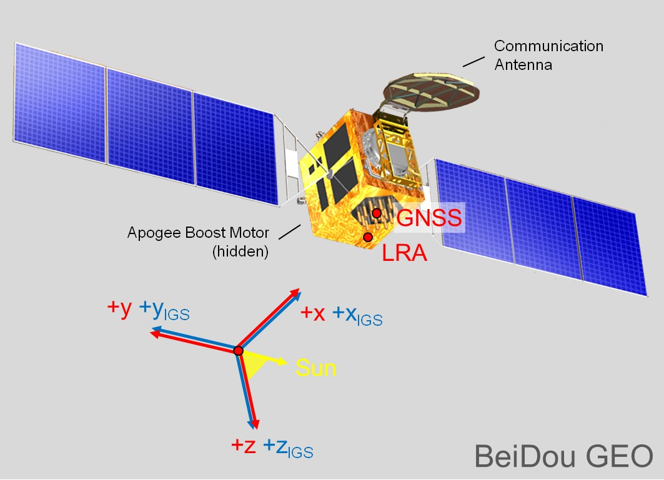
BeiDou GEO Satellite
Source: http://mgex.igs.org/IGS_MGEX_Status_BDS.html
The first generation of the system is known as BeiDou-1. It is a regional satellite navigation system that services a portion of the Earth from 70°E longitude to 140°E longitude and from latitude 5°N to 55°N. It relies on 3 satellites with 1 backup. The first satellites were launched into geostationary (GEO) orbits in 2000; BeiDou-1A at 140º E longitude and BeiDou-1B 80º E longitude. A third satellite, BeiDou-1C joined them 3 years later at110.5º E longitude. With the launch of the fourth, BeiDou-1D in 2007 the first BeiDou-1 system was operational, regionally.
Beidou-2 (aka Compass) is the second generation of the BeiDou Navigation Satellite System (BDS). In 2007, Xinhua, the government news agency, announced that the People’s Republic of China National Space Administration would launch two more GEO satellites to open the way to a global Chinese Satellite Navigation system to replace the regional BeiDou-1.
The first BeiDou-2 satellite, a medium Earth orbit (MEO) satellite named Compass-M1, was launched into a circular orbit at 21,500 km at an inclination of 55.5º. Similar satellites followed; and between 2007 and 2012, there were 5 MEO satellites with sequential names from Compass-M1 to M6 (without an M2) launched. During the period from 2009 to 2012, the 6 GEO BeiDou-2 satellites with sequential names from Compass-G1 to G6 were launched. Their positions are at 58.75°E longitude (G5), 80.0°E longitude (G6), 110.5°E longitude (G3), 140.0°E longitude (G1), 160.0°E longitude (G4). The G2 satellite is inactive.
From 2010 to 2011, the 5 high Earth orbit (HEO) BeiDou-2 satellites with sequential names from Compass-IGS01 to IGS05 were launched and achieved an altitude of approximately 38,000 km. The acronym IGOS means inclined geosynchronous orbit satellites. The IGS01, IGS02 and IGS03 satellite are at ~120°E. IGS04 and IGS05 are at ~95°E. All the IGSO satellites have an inclination of 55° and are arranged so that one of them is always over the Chinese region. The system began trial operations in late 2011 and followed with service to the region bounded by 55°E longitude to 180°E longitude and latitude 55°S to 55°N.

BeiDou Constelltion
Source: https://www.cosmos.esa.int/documents/13611/3707333/20200213_Ventura_Trav...
The BeiDou Constellation is operational. The constellation occupies six orbital planes. There are 44 satellites on orbit; 7 of them are geostationary satellites (GEO). 37 are non-stationary. The 37 non-stationary satellites include 27 in medium Earth orbit (MEO). 10 are orbiting at inclined geosynchronous orbits (IGSO). All the satellites will have a phased array antenna, on-board retro-reflector, a C-band horn antenna, and an S/L-band dish antenna.
BeiDou’s Signals and Services

BeiDou satellites currently transmit signals in three bands; B1 (1561.098 MHz), B1-2 (1589.742 MHz), B2 (1207.14 MHz) and B3 (1268.52). These bands overlap Galileo on E2-L1-E1, E5B, and E6 respectively. Each of the Beidou signals in these bands have an I (in-phase) and Q (quadraphase) component in quadrature with one another. BeiDou’s multiple access system is CDMA. The modulation scheme is quadraphase shift key (QPSK). The BeiDou Radio Navigation Satellite Service (RNSS) has 5 new global signals; B1C (1575.42 MHz), B1A (1575.42 MHz), B2a (1176.45 MHz), B2b (1207.14 MHz) and B3A (1268.52). These bands overlap GPS L1 and Galileo on E2-L1-E1: GPS L5 and Galileo E5a: Galileo E5b, and Galileo E6 respectively.

Radio Determination Satellite Service (RDSS) and Radio Navigation Satellite Service (RNSS).
https://onlinelibrary.wiley.com/doi/abs/10.1002/navi.291
The future BeiDou is expected to support two different kind of general services: Radio Determination Satellite Service (RDSS) and Radio Navigation Satellite Service (RNSS). The RDSS will include a short message communication (guaranteeing backward compatibility with BeiDou-1). A satellite-based 2-way short message service in China and the surrounding areas (75 -135 ° E 10 -55° N) with a power of < 3W and a capacity of more than 10 million messages/hr using 3 GEO satellites. The RDSS Characteristics will include a global message service using inter-satellite crosslinks with 10W of power and a capacity of 200,000 messages/hr using 14 MEO satellites. The Radio Navigation Satellite Service (RNSS) is very similar to that provided by GPS and Galileo and is designed to achieve a similar performance.

Satellite Based Augmentation Service (SBAS).
https://www.shangyexinzhi.com/article/2004171.html
It will also include a Satellite Based Augmentation Service (SBAS). Space Segment - three BDS-3 GEO satellites (80°E,110.5°E,140°E); Ground Segment - Operation and Control Center, Data Centers, Uplink Stations, Monitoring Stations; User Segment - BDSBAS terminals can receive RNSS navigation messages and wide area differential integrity information broadcast by GEO satellites

Click here to see a text description.
| Signals | Carrier Frequency (MHz) | Chip Rate (cps) | Multiple Access Scheme | Bandwidth (MHz) | Modulation Type | Service Type | Minimum Received Power |
|---|---|---|---|---|---|---|---|
| B1(I) | 1561.098 | 2.046 | CDMA | 4.092 | QPSK | Open | -163 dbW |
| B1(Q) | 1561.098 | 2.046 | CDMA | 4.092 | QPSK | Authorized | -163 dbW |
| B1-2(I) | 1589.742 | 2.046 | CDMA | 4.092 | QPSK | Open | -163 dbW |
| B1-2(Q) | 1589.742 | 2.046 | CDMA | 4.092 | QPSK | Authorized | -163 dbW |
| B2(I) | 1207.14 | 2.046 | CDMA | 24 | QPSK | Open | -163 dbW |
| B2(Q) | 1207.14 | 10.23 | CDMA | 24 | QPSK | Authorized | -163 dbW |
| B3 | 1268.52 | 10.23 | CDMA | 24 | QPSK | Authorized | -163 dbW |
There are two service types. The Open Service is available to the public and offers an autonomous (not differentially corrected) positional accuracy of 10m, 0.2 m/s velocity accuracy, and timing accuracy within 20 nanoseconds. The Authorized service is not available to the public. It is available to the military, specifically the militaries of China and Pakistan.
There are two navigation messages available from the BeiDou satellites. The MEO satellites and the IGSO satellites transmit the D1 NAV message, which is similar to the GPS NAV message. The D1 message has 30-bit words and 10 word subframes, i.e., 300 bits. It is broadcast at 50 bps and has adequate capacity for almanac data for 30 satellites. It also includes time offset information for UTC and other GNSS system clocks.
The GEO satellites transmit the D2 message. It also has 30-bit words and 10-word subframes but is broadcast at 500 bps. The D2 message includes pseudorange corrections to satellites in subframes 2 and 3 with enough capacity to accommodate corrections for 18 satellites. D2 has ionospheric corrections and clock corrections to other GNSS systems in subframe 5. This provides a unique service planned for the BeiDou Control/Ground Segment that has not been incorporated into other GNSS systems, a wide area differential correction available directly from the constellation rather than from a separate system. The BeiDou Ground Based Enhancement System (BGBES) network includes 150 reference stations; information from these stations provided is processed in the BeiDou Control/Ground segment and the resulting corrections are sent to the BeiDou GEO satellites. Those corrections are then broadcast by the GEO satellites via the D2 NAV message to the BeiDou user’s terminals (receivers). In other words, the GEO satellites provide satellite based augmentation (SBAS) for users in the region between 70° E. Longitude to 145° E. Longitude and 5° N. Latitude to 55° N. Latitude. While the BeiDou’s open service is said to offer positional accuracy of ~10m, the differentially corrected is expected to produce ~1m.
Within the same region, BeiDou also provides a short message service (SMS). Users are enabled to send up to 120 Chinese characters in each message.

Beidou Control Segment
http://www.satnews.com/story.php?number=1934630546
BeiDou’s Control/Ground Segment
The BeiDou Control/Ground Segment is comprised of a Master Control Station (MCS), two Upload Stations (US) and a network of 30 widely distributed Monitoring Stations (MS). Similar to the control of other GNSS constellations, the MCS receives data from the Monitoring Stations, which track the constellation continuously. The Upload Stations send the data generated information by the MCS to the satellites.
The MCS is responsible for the operational control of the system, including orbit determination, navigation messages, and ephemerides which are based on the China Geodetic Coordinate System 2000 (CGCS2000). CGCS2000 is the coordinate framework of the BeiDou System and is within a few centimeters of ITRF. The MCS also coordinates mission planning, scheduling, and time synchronization with BeiDou Time (BDT). BDT is synchronized within 100ns of UTC (NTSC) as maintained by National Time Service Center, China Academy of Science. BDT does not incorporate leap seconds. The leap second offset is broadcast by the BeiDou satellites in the navigation message. The initial epoch of BDT is 00:00:00 UTC on January 1, 2006. The offset between BDT and GPST/ GST is also to be measured and broadcasted in the navigation message.
The Quasi-Zenith Satellite System and IRNSS also known as NavIC

Click here to see a text description.
Quasi-Zenith Satellite System (QZSS)
- 3 Orbital Planes
- 3 Satellites
- ~40 degree inclination angle
- Altitude
The first demonstration satellite of the Japanese Quasi-Zenith Satellite System (QZSS), QSZ-1 was launched in 2010 by the Japan Aerospace Exploration Agency (JAXA) from the Tanegashima Space Center. It is expected to have a design life of 10 years. The system is nicknamed Michibiki, meaning guide. Three more satellites were launched in phase two in 2017. They include 2 additional quasi-zenith satellites, QZ-2 and QZ-3 and 1 geostationary satellite, QZ-4 which is on orbit at the equator. The 4 satellite constellation is planned to increase to 7 satellites in the future.

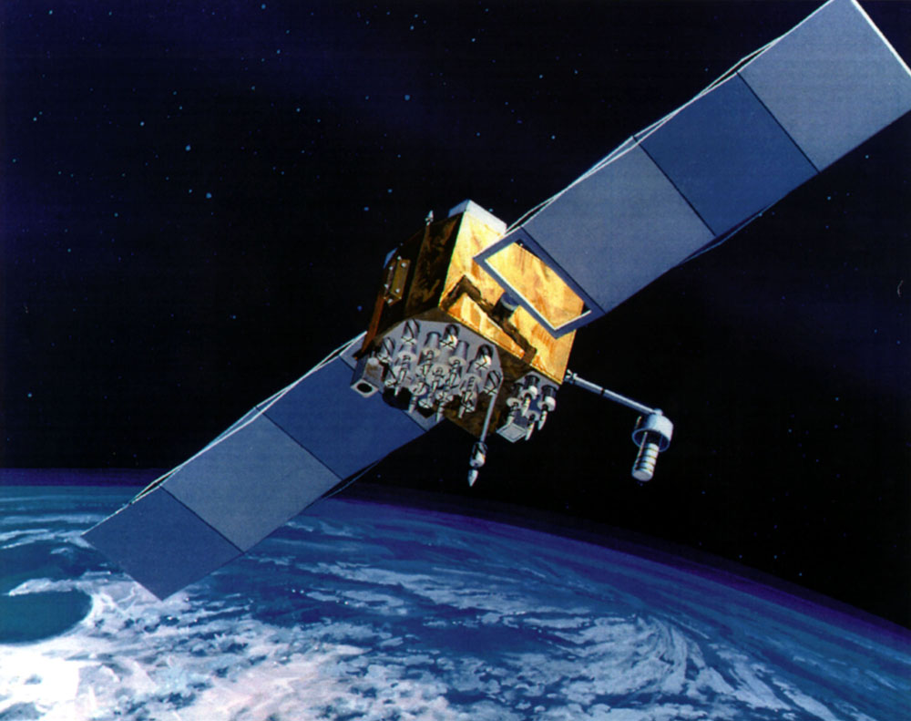
QZSS is intended to provide satellites in highly elliptical orbits (HEO) that are inclined and geosynchronous. The orbits are designed, so the satellites will always be available at high elevation angles that are almost directly overhead in Japan, Oceania and East Asia. This is the origin of the term quasi-zenith. They orbit at ~32000 km to ~40000km. And all follow the same asymmetrical figure-8 ground track in the region. QZSS is primarily a multi-satellite regional augmentation system (SBAS). The system offers both Sub-meter Level Augmentation Service (SLAS) and Centimeter Level Augmentation Service (CLAS). Service began November 1, 2018.

The objective is to improve satellite positioning, navigation and timing services in urban canyons and mountainous areas in the region. The system is designed to improve the positioning of GPS and Galileo receivers. The system transmits 6 signals; L1-C/A, L1C. L2C, L5, L1-SAIF and LEX. The first 4 on the list are the familiar GPS signals. The others are unique to QZSS. L1-SAIF (Submeter-class Augmentation with Integrity Function) is broadcast at the L1 frequency, 1575.42 MHz. It is interoperable with GPS and is intended to provide a sub-meter correction signal to users. Another unique signal to be broadcast by QZSS is LEX (L-band Experiment) at 1278.75 MHz. LEX is being developed to provide high accuracy positioning that is interoperable with Galileo E6. QZSS will broadcast multiple frequency signals and also provide a short message service (SMS) as does the Chinese BeiDou system. There may be user fees developed for these signals and services.
The commercial portion of the QZSS operation will be managed by Quasi-Zenith Satellite System Services Inc. (QSS). The system integration, research and development of the QZS Bus, the ground segment, etc. will be under JAXA’s control.

QZSS Control Segment
Source: https://earth.esa.int/web/eoportal/satellite-missions/q/qzss
QZSS Control/Ground Segment
The Master Control Station (MCS) develops the ephemerides, time, and navigation messages which are uploaded to the QZS satellite constellation by the main Telemetry, Tracking, and Command (TT&C) ground station in the Okinawa prefecture. Other monitoring stations on Japanese territory are at Ogasawara, Koganei, and Sarobetsu. However, there are also monitoring stations in areas governed by other nations. They are on Hawaii, Guam, Bangkok, Bangalore, and Canberra. The QZSS ground segment also includes laser ranging and tracking control stations (TCS). The main TCS station is at JAXA's Tsukuba Space Center.
The reference system for QZSS is the Japanese Satellite Navigation Geodetic System (JSG) which is quite near The International Terrestrial Reference System (ITRS). The time reference for QZSS is known as Quasi-Zenith Satellite System Time (QZSST). The system does not use leap seconds. The duration of the second in this system is the same as that in TAI (International Atomic Time).
IRNSS also known as NavIC

IRNSS Satellite
The building of the Indian Regional Navigation Satellite System (IRNSS) was authorized by the Indian government in 2006. When fully developed by the Indian Space Research Organization (ISRO), the constellation will provide position, navigation, and timing service in a region from Latitude 30° S. Latitude to 50° N. Latitude and from 30° East Longitude to 130° East Longitude. The region embraced is approximately 1500 kilometers around India. The constellation is also known as NavIC (Navigation with Indian Constellation; also, nāvik 'sailor' or 'navigator' in Sanskrit, and many other Indian languages).
The IRNSS constellation is comprised of 7 operational satellites. All the satellites will be continuously visible to the extensive Indian control segment’s 21 stations located across the country, including the Master Control Center (MCC) at Hassan, Karnataka. They are named with the prefix IRNSS-1. The constellation includes 3 of the 7 satellites in geostationary orbits at 32.5º East Longitude, 83º East Longitude and 131.5º East longitude and 4 of the 7 satellites are in geosynchronous orbits of 24,000 km apogee with an inclination of 29°. The small inclination is appropriate to the coverage of India, as the nation is located in the low latitudes. The equator crossing of 2 of the geosynchronous satellite is at 111.75º East Longitude and 2 crosses the equator at 55º East Longitude.
IRNSS-1A was launched in 2013 and is now in partial failure. IRNSS-1B and IRNSS-1C were launched in 2014. All three were launched from the Satish Dhawan Space Centre at Sriharikota, India. They carry a rubidium clocks, corner cube retro-reflectors for laser ranging and a C-band transponders. They broadcast in the L5 band (1176.45 MHz) with a bandwidth of 24 MHz and S band (2492.028 MHz) with a bandwidth of 16.5 MHz. They have a ten-year design life. IRNSS - 1D was launched in 2015. IRNSS-1E through 1G were launched in 2016. IRNSS-1H failed to make orbit. IRNSS-1I was launched in 2018.
IRNSS provides two levels of service, a public Standard Positioning Service (SPS) and an encrypted Restricted Service (RS). Both will be available on L5 and on the S band; however, the SPS signal is modulated by BPSK at I MHz and the Restricted Service will use BOC (5, 2). The navigation signals is broadcast on the S-band.


The Future

The Future
So, what is coming? Someday, there may be as many as 130 navigation satellites aloft. They will be from GPS, GLONASS, Galileo, BeiDou, QZSS, IRNSS, and perhaps others. If so, the systems will provide users with quite a variety of signals and codes. The availability of many more satellites will enable new applications in areas where their scarcity has been a hindrance. For civil users, new signals will provide more protection from interference, ability to compensate for ionospheric delays with pseudoranges, and wide-laning or even tri-laning capabilities. For military users, there will be greater anti-jam capability and security. For everybody, there will be improvement in accuracy, availability, integrity, and reliability. So, it is no surprise that there is great anticipation from a business perspective, but from a user’s point of view, the situation is not unlike the advent of GPS years ago. Much is promised, but little assured. New capabilities will be available, but exactly what and exactly when is by no means certain.
More satellites will be above an observer’s horizon. GPS and GLONASS together now provide the user with ~2 times the satellites than does GPS alone. If GPS, GLONASS, and Galileo are considered together, there will be ~3 times more. If BeiDou is added to the mix, there will be ~4 times more satellites that will be available to a user. In a sense, the more satellites, the better the performance, particularly among trees and in urban canyons, those places where signals bounce and scatter, and multipath abounds. For example, with the 6 satellites in a window available to a GPS receiver on the left side of the Urban Canyon figure below, the user may be able to increase the mask angle to decrease the multipath and still have 4 satellites to observe. Imagine if there were 12, 18, or even 24 satellites in the picture, and you can see how more satellites can mean better accessibility in restricted environments.

More satellites also mean more measurements in shorter time and that means observation periods can be shortened without degrading accuracy, in part because interference can be ameliorated more easily. With more satellites available, the time to first fix for carrier-phase receivers, the period when the receiver is solving for the integers, downloading the almanac and so forth, also known as initialization, will be shortened significantly. And fixed solution accuracy will be achieved more quickly. Today, dual-frequency carrier-phase solutions are accurate but noisy; but with the new signals available on L2C, L5, and other GNSS signals, dual-frequency solutions will be directly enhanced. While a GNSS capable receiver may offer a user improved availability and reliability, it may not necessarily offer higher accuracy than is available from GPS. However, the achievement of high accuracy more conveniently and in more places— that seems to be within reach with GNSS. It also means better ionospheric correction. Remember, the ionospheric delay is frequency dependent.
The algorithms currently necessary for the achievement of high accuracy with carrier-phase ranging may be simplified, since many of the new GNSS signals will be carrying a civilian code. Generally speaking, code correlation is a more straightforward problem than is carrier differencing. This may lead to less complicated receivers. This presents the possibility that they will be less expensive.
Also, the more diverse the maintenance of the components of GNSS, the less chance of overall system failure; the United States, Russia, the European Union, and China all have infrastructure in place to support their contribution to GNSS. Under such circumstances, simultaneous outages across the entire GNSS constellation are extremely unlikely.
Discussion
Discussion Instructions
To continue the discussion begun by this lesson, I would like to pose this question:
There is much discussion about reliance on GPS/GNSS and concern about security. It has become essential to a wide variety of critical functions. Backup for, or perhaps replacement of the system are contemplated. What are your thoughts on the subject?
To participate in the discussion, please go to the Lesson 10 Discussion Forum in Canvas. (That forum can be accessed at any time by going to the GEOG 862 course in Canvas and then looking inside the Lesson 10 module.)
Summary

Thank you very much for spending this time with me. I appreciate it. It's been a thrill, and I have enjoyed it. Thank you.
This is the conclusion of this course. Before you sign off, be sure to double-check the Lesson 10 Checklist to make sure you have completed all of the activities listed there.