The Nexview 3D Interferometer

Optical Profilers
Optical profilers are interference microscopes, and are used to measure height variations – such as surface roughness – on surfaces, with great precision, using the wavelength of light as the ruler.
Optical profiling uses the wave properties of light to compare the optical path difference between a test surface and a reference surface. Inside an optical interference profiler, a light beam is split, reflecting half the beam from a test material which is passed through the focal plane of a microscope objective, and the other half of the split beam is reflected from the reference mirror.

Constructive interference occurs when the phase difference between the path lengths is a multiple of 2π, whereas destructive interference occurs when the difference is an odd multiple of π.This creates the light and dark bands known as interference fringes.
Since the reference mirror is of a known flatness, that is, it is as close to perfect flatness as possible, the optical path differences are due to height variances in the test surface.
This interference beam is focused into a digital camera, which sees the constructive interference areas as lighter, and the destructive interference areas as darker.
In the interference image (an "interferogram") below, each transition from light to dark represents one-half a wavelength of difference between the reference path and the test path. If the wavelength is known, it is possible to calculate height differences across a surface, in fractions of a wave. From these height differences, a surface measurement – a 3D surface map, if you will – is obtained.
Hypothetically, if the wavelength is 500 nanometers, one could estimate the distance of slope over a full wavelength by looking at the light and dark interference bands – known as interference fringes – in an interferogram. Optical profilers calculate these differences much more accurately than is possible by visual methods.

In practice, an optical profiler scans the material vertically. As the material in the field of view passes through the focal plane, it creates interference. Each level of height in the test material reaches optimal focus (and therefore greatest interference and contrast) at a different time. With well-calibrated optical profilers, accuracy well below a nanometer is possible.
Optical profiling can be used to measure surface finish, roughness, and shape on many surfaces, so long as enough light is reflected back into the objective from the surface.
Much of the content was taken from Zygo's Optical Profiler Basics Webpage
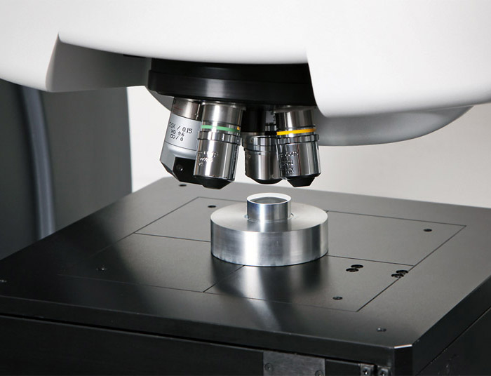
The Instrument and lenses
The Nexview interferometer layout

The Zygo surface profilers use interferometers built into the microscope objectives, in either a Michelson (left) or Mirau (right) configuration.
The objectives are calibrated so that the point of zero optical path difference (zero OPD) is the same as the focal distance, i.e., the distance from the beamsplitter to the reference surface is the same as the focal length. This means fringes will appear when the test part is in focus. You will hear working distance, focal distance, and zero OPD used interchangeably during training.

Breaking the Instrument
Optical profilometry is a non-contact imaging technique. The only way to break the instrument is to:
- drive any of the objectives into your sample (odd shaped samples must watch out for all the objectives on the turret!).
- make contact with the objectives on the turret while loading or manipulating your sample. All contact is bad, even the slightest bump or brush.
- change objectives without raising Z, allowing clearance for torrent rotation. The objectives on the turret are not parfocal, You must raise Z in order to change lenses.

The Joystick
The joystick controls the manual motion of the stage in X, Y, Z, Pitch, and Roll.
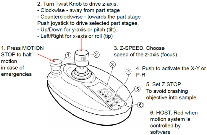
- Fast, Medium, and Slow buttons (3) control the Z-speed (2).
- X-Y or (P)itch-(R)oll control of stage. 200 mm of travel in X and Y and +/- 4 degree of tilt.
- Z-stop setting to avoid crashing objectives into sample.
Spatial Sampling
The detector is a CCD camera with a finite number of pixels. Thus, the optical resolution is also limited by the spatial sampling of the system, i.e., the field of view divided by the number of pixels.

Spatial Sampling = FoV / 1024
Field of View and Numerical Aperture
Field of View
The Field of View (FoV) is the diameter of the circle of light that you see when looking into a microscope. The higher your magnification, the smaller the microscope field of view will be.
The benefits a microscope objective
The imaging system of the Nexview 3D is a microscope objective, which gives the two-fold benefit of:
- higher magnification for small features;
- measurement of rough and sloped surfaces due to higher numerical aperture.

Numerical Aperture (NA)
In optics, the numerical aperture(NA) characterizes the range of angles over which the system can accept or emit light. When the light hits a surface which is highly sloped, it can be reflected to not return up the optical system, and nothing will be detected. This means that higher NA objectives can measure steeper slopes.

Optical Resolution
Optical resolution: the Airy disk
Diffraction of light through a circular aperture (like a lens) limits the resolution of any optical system. The best focus of a point source of light from a lens system will form an Airy disk due to this diffraction, rather than the idealized point source.

Optical resolution is usually defined as the ability to distinguish two objects which are close together, which is difficult due to the overlap of the Airy disks.
Common criteria for the resolution R:
- The Rayleigh Criterion: R = 0.61λ/NA
- The Sparrow Criterion: R = 0.5λ/NA (used by Zygo)
The effect of diffraction will be a smoothing of features which are too small to resolve sharply.
Note: This resolution is in the lateral (parallel to the focal plane) direction – it is not related to the vertical resolution of the Nexview's measurements.

Optical Resolution of our Objectives
- 2.75x~ 3.563μm
- 10x ~ 950 nm
- 20x ~ 713 nm
- 50x ~ 518 nm
Effects of Optical Resolution and Spatial Sampling on Data
Review:
Optical Resolution = 0.5λ/NA
Spatial Sampling = FOV/1024
Effect of changing optical resolution and spatial sampling
Below is an example of the effect of optical resolution and spatial sampling on information calculated from the surface data. It compares data collected with a 2.75X (NA = 0.08, FOV = 3.00 mm) objective with that from a 10X (NA = 0.3, FOV = 0.83 mm) objective. Since both the NA and the FOV change, our optical resolution and spatial sampling change. The 10X objective is able to capture finer details, and we see the surface roughness increase.
- Sa = surface arithmetic average roughness
- Sq = surface RMS roughness
- Sz = Peak to Valley difference

Effect of changing spatial sampling while using the same optical resolution
In the below example, the optical resolution is kept the same, both are using the 50X objective (NA = 0.55). However, we are using the internal magnification (0.5X, 1.0X, 2.0X) to change the FOV, which affects the spatial sampling. Even though it has the same resolution, the results collected are affected by the different spatial sampling.
- Sa = surface arithmetic average roughness
- Sq = surface RMS roughness
- Sz = Peak to Valley difference

Note
Be very careful when comparing data from different scans. The above examples illustrate that numerical values from surfaces should only be compared if they were collected using the same optical resolution and spatial sampling.
Working Distance
The working distance (W.D.) is determined by the linear measurement of the objective front lens to the focal plane. In general, the objective working distance decreases as the magnification and numerical aperture both increase.

The working distance is the distance from the front of the lens to the focal plane. The objectives are designed that this is also where zero OPD occurs. Because of this, the terms W.D., focus, and zero OPD are often used interchangeably.
Z-Stop
The Z-Stop protects the optical profilometer in the Z direction. It needs to be set for each sample, with care taken to set a proper distance.

Set Z-Stop (CRITICAL)
- Verify the working distance of the objective. (See table below.)
- Check Z-Stop status (what color is Z-stop light on joystick?).
- Red = At Z-stop position.
- Green = Above Z-stop position.
- Flashing Red = No Z-stop is set. USE EXTREME CAUTION (instrument will beep as you move in Z).
- Only pay attention to the space between the objective and the top of your sample. No need to look at the PC, your cell phone, your friend next to you. Just focus on the objective-sample gap.
- The ideal Z-stop position is defined as a distance between objective and sample surface that is less than the working distance and allows for the scan to reach just below the lowest region of the surface. Too low a Z-stop can put the instrument at risk; a Z-stop too close to the Working Distance could lead to software errors when you try to scan.
- Use Fast only at distances greater than 20mm from the sample. Press Z-stop button so the light is flashing RED and begin a downward focus until you arrive at approximately 20mm. Push Medium and continue towards the surface until an appropriate Z-stop position. Never use “FAST” speed when nearing sample surface (<20mm)
- Press Z-stop so the light is now solid RED.
- Use focus aid and raise Z to focus.
What is a good Z-Stop position?
The simple answer here is one that allows the instrument to scan low enough to scan through all parts of your surface AND prevents the instrument from being driven into your sample. Below are illustrated examples of an improper and proper Z-stops.


Most important thing to remember when setting the Z-Stop is to remember you do this manually by watching the objective and your sample directly. It is never to be set watching the computer screen with the software.

Nexview Objective Selection Guide
Objectives highlighted in yellow are the ones currently installed on the Nexview 3D turret.

The Nexview 3D has 4 objectives on the turret and 3 internal magnifications, giving 12 FOV (highlighted in the middle of the above image), some of which overlap.
So, which do you choose?
Most often it is the size of what you are trying to measure which determines the FOV you want to work at.
But what about the overlapping fields of view; which objective should I use?
In the case of overlapping FOV; for example, the 10X objective can be used as a 5X, 10X, or 20X, and the 20X objective can be used as a 10X, 20X, or 40X. They both have 10X and 20X options; so, which do I choose? The 20X is the choice over the 10X on flatter samples as it has the better NA, which means you have better optical resolution. However, the 10X has a much further working distance and can be useful on rougher samples when we can't use the 20X.
These are the things you consider when making your objective choice.
Pitch, roll, and null
The lateral/Y axis, or pitch axis is an imaginary line running horizontally across the sample through the center of gravity. A pitch motion is an up-or-down movement of the front or back of your sample as mounted on the stage.
The longitudinal/X axis, or roll axis is an imaginary line running horizontally though the length of the sample through its center of gravity. A roll motion is a side-to-side movement or tilting left or right of your sample as mounted on the stage.
To "null" the fringes is to adjust the pitch and roll of your sample so it is parallel to the plan of the interference fringes, which is perpendicular to the Z-scan axis.
Nulling the fringes predominantly helps you with minimizing the scan length needed to measure your surface.

An example for Smooth Flat Surfaces
To "null" the fringes is to adjust the pitch and roll of your sample so it is parallel to the plan of the interference fringes, which is perpendicular to the Z-scan axis.

The cartoons to the right show the impact on scan length when a flat part is nulled properly (cartoon on the right with the small green scan length outlined is nulled properly). If the differences in scan length on in a few μm to tens of μm it likely doesn't matter much. If the differences are in the 100s of μm, it will greatly affect your collection time and care should be taken to null the surface as best you can.
For a Smooth Flat Part, adjust for high contrast and the least number of fringes. On very flat parts, it is possible to null the surface such that the fringes take up the entire field of view
Below is a video showing the actual field of view (right) and a cartoon (left) depicting what is happening on a tilted smooth flat part as the instrument is moved up in Z with the joystick. Notice how the fringes travel across the field of view from upper right to lower left. The fringes indicate that not only is the sample tilted, the direction of travel describes how it's tilted. The fringe travel indicates, in this example, that the front left corner of the stage is higher.
Nulling the stage for a smooth flat part gets the sample surface and the Z-travel perpendicular, which means the surface is parallel to the fringes now. As the instrument is moved up in Z now, the fringes can be seen individually as they flash by.
An example for Textured Surfaces
To "null" the fringes is to adjust the pitch and roll of your sample so it is parallel to the plan of the interference fringes, which is perpendicular to the Z-scan axis.

Textured surfaces are very similar to flat surfaces, though it can be harder to see the trend in the tilt of the sample. The goal is to null the overall sample tilt to minimize the scan length.
On Textured or Rough Flat Part the fringes are in smaller isolated areas. Center the fringes and adjust the focus between the high and low fringes. The distinct lines that were seen for smooth surface are broken up with the varying topography of a rough or textured surface. Nulling the fringes involves adjusting the fringes so they enter and leave the field of view without any discernible trend in X or Y tilt.
Below is a video showing the actual field of view (right) and a cartoon (left) depicting what is happening on a tilted textured or rough part as the instrument is moved up in Z with the joystick. Notice how the fringes travel across the field of view from lower right to upper left. The fringes indicate that not only is the sample tilted, the direction of travel describes how it's tilted. The fringe travel indicates, in this example, that the back left corner of the stage is higher.
Nulling the stage for a textured or rough part also gets the sample surface and the Z-travel perpendicular, which means the surface is parallel to the fringes now. As the instrument is moved up in Z now,fringes enter and leave the field of view without any discernible trend in X or Y tilt.
An example for Curved Surfaces
To "null" the fringes is to adjust the pitch and roll of your sample so it is parallel to the plan of the interference fringes, which is perpendicular to the Z-scan axis.

On a Spherical Part, adjust the stage and the focus to center the circular fringe pattern. This can be done by moving in X/Y or in P/R, depending on what you are trying to measure. Depending on the curvature of the sample, nulling a spherical sample can significantly reduce collection time.
Below is a video showing the actual field of view (right) and a cartoon (let) depicting what is happening on a curved part as the instrument is moved up in Z with the joystick. Notice how the fringes travel across the field of view from right to left. The fringes indicate that not only is the sample offset, the direction of travel describes how it's offset. The fringe travel indicates, in this example, that the back sample curvature continues to rise to the left. Either X/Y or P/R can be adjusted to center the circular pattern depending on the users specific needs.
Nulling the stage for a curved part minimizes the total sample height within the field of view. As the instrument is moved up in Z now, the fringes go through a circular, bullseye pattern centered in the field of view.
Relationship between working distance, Z-stop, and scan length
Review of some important concepts

The working distance is the distance from the front of the lens housing down to the focal plane of the objective. We commonly use working distance, focal plane, and zero optical path difference interchangeably. The focal plane of the objective must scan all the way through the sample surface (from above, down through, and then below the highest and lowest parts of the surface in the FoV of the scan or stitch).
Z-Stop
The Z-Stop is a hard stop for both the user and the software, set before working in the software, to allow the focal plane to scan through the required scan length but prevent any part of the instrument from making contact with any part of the sample or sample mounts that may be in use.

In the above image, we have three different Z-stop (denoted by the red line) settings. On the left, the Z-stop is set too close to the surface, and you will not get any good data. In the middle, the lower Z-stop allows you to collect some information from the higher parts of the sample surface, but it does not take into account the proper distance the width of the fringes must travel through to reach the lowest part of the sample. The image on the left shows a Z-stop that not only allows the instrument to scan the width of the fringes through all of the surface topography, but also protects the objective from being driven into the sample by the user or the software.
Scan Length
Scan length is discussed in the section on MX™ measure tab, but we will take this into consideration here for a moment to get you thinking about things to come.
Once you have a proper Z-stop set. Setting up the proper scan requires the user to set up a proper scan start position and scan length so the width of the fringes can be scanned entirely through the surface topography. An illustration of what the system looks like scanning is depicted below. Notice how the instrument moves with respect to start and end scan. This will be covered in more detail in the next sections.
