Prioritize...
In this section, you should focus on the interpretation of multispectral imagery, and be able to identify clouds as low, middle, or high based on the color scheme used in the three-channel color composites showin in this section. Furthermore, you should be able to use multispectral imagery to identify the low-level circulation of a tropical cyclone when it's exposed.
Read...
So far, the satellite remote sensing techniques that we've covered have originated from geostationary satellite data. For example, geostationary satellites effectively have the "market cornered" on retrieving cloud-drift winds because satellites in geostationary orbit have a fixed view. That fixed view makes the creation of satellite loops, from which CDWs are retrieved, feasible. Polar-orbiting satellites, however, do not have a fixed view, and without the ability to create loops of imagery from polar orbiters, they're not useful for retrieving CDWs.
Nonetheless, polar orbiters play a pivotal role in the remote sensing of tropical weather systems. You may recall that polar orbiters fly at much lower altitudes than geostationary satellites and are "sun synchronous" (meaning that they ascend or descend over a given point on the Earth's surface at approximately the same time each day). Multiple fleets of polar orbiting satellites currently circle the Earth (more in the Explore Further section below), and, like GOES, they provide multispectral (or "multi-channel" -- using multiple wavelengths of the electromagnetic spectrum) scans of the Earth and the atmosphere. Over the next few sections we'll explore the multispectral capabilities of polar orbiters and the roles that remote sensing by these satellites play in tropical weather analysis and forecasting.
Among the key instruments aboard the NOAA fleet of polar orbiters(link is external) are the Advanced Very High Resolution Radiometer (AVHRR), and the Visibile Infrared Imaging Radiometer Suite (VIIRS). These instruments collect data at multiple wavelengths ("channels") across the visibile and infrared portions of the electromagnetic spectrum, which allows us to collect information about day and nighttime cloud cover, snow and ice coverage, sea-surface temperatures, and land-water boundaries. If you're interested in learning more about the details of these instruments or their applications, you can read more about the AVHRR(link is external) and VIIRS(link is external). In case you're wondering about the reference to "very high resolution" in AVHRR, you may be interested in exploring the topic of resolution more in the Explore Further section below.
These instruments' broad capabilities for detecting clouds during the day and at night come from the fact that they scan at multiple wavelengths across the visible and infrared portions of the electromagnetic spectrum. Radiation detected across several channels can be combined to create composite images that provide additional information to weather forecasters. One product that has long been common in tropical forecasting is a three-channel color composite like the one below of Hurricane Katrina captured by NOAA-16's AVHRR at 2011Z on August, 28 2005.
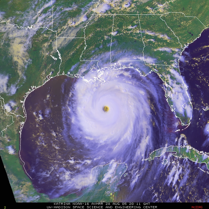
The yellowish appearance of Katrina's eye really stands out, doesn't it? That yellowish shading corresponds to low-topped, relatively warm clouds within Katrina's eye (remember that the eye of a hurricane often contains low clouds). Meanwhile the thick, tall convective clouds with cold tops surrounding the eye appear bright-white on this three-channel color composite, and high, thin cirrus clouds appear blue/white.
In terms of tropical forecasting, multispectral satellite images of tropical cyclones can sometimes be very helpful in assessing the tendency of a system's intensity. Focus your attention on the daytime, three-channel color composite of Tropical Cyclone Heta (07P) at approximately 00Z on January 8, 2004 (on the left below). At the time, Heta's maximum sustained winds were 35 knots, with gusts to 45 knots. Thus, Heta had minimum tropical-storm strength as it weakened over the South Pacific Ocean.
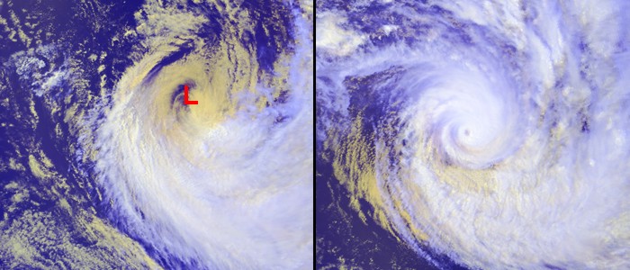
The fact that the clouds near Heta's center appear yellowish on this image indicates low clouds and a lack of deep convection near its core. Without organized deep convection near its core, Heta was in a sorry state indeed since there was no catalyst for deep (but gentle) subsidence over its center. Thus, Heta could not maintain formidable strength. However, just two days earlier on January 6, 2004, (image above right) deep convection surrounded the eye of Tropical Cyclone Heta as evidenced by the very bright white clouds near the eye. At the time, Heta had maximum sustained winds of 125 knots.
Furthermore, when a tropical cyclone is highly sheared, the color scheme of three-channel color composites can really expose the structure of the storm. For example, check out this loop of three-channel color composite images of Tropical Depression 8 in the Atlantic from August 28, 2016. Not long after the storm was classified as a depression, the deep convective clouds (bright white) got displaced to the northwest thanks to strong southeasterly wind shear. The yellow swirl of clouds left behind clearly marks the storm's low-level circulation. It was obviously not a "healthy" storm at this time.
How does it work?
How are these useful three-channel color composites created? The process really isn't too complex, and is outlined by the graphics below. We'll use the details of the AVHRR for our example. First, we start with standard grayscale visible (channel 1), near (or "shortwave") infrared (channel 2), and infrared (channel 4) images (check out the top row of satellite images in the graphic below). Next, we apply a red filter to the visible image, a green filter to the near-infrared image, and a blue filter to the infrared image, and we get strange looking satellite images like the ones in the second row of the graphic below. But, if we combine those "false-color" images together, we get a three-channel color composite!
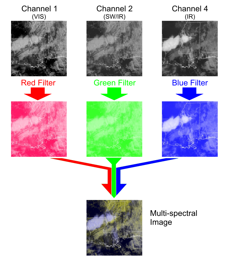
Breaking down this three-channel color composite helps us to understand why high, thin clouds appear in blue on the final product -- they're brightest on the infrared channel (which had blue hues added to it). Meanwhile, tall, thick convective clouds that show up bright white on the final product are bright on the individual images from all three channels, and low clouds appear yellow because they're brightest on the visible (red) and near-infrared (green) images. The combination of green and red provides the yellow shading (if you're unfamiliar with why yellow results, you may want to read about additive color models(link is external) if you're curious).
Similar satellite composites can be created from data collected by geostationary satellites, too, by adding red and green filters to visible imagery and a blue filter to infrared imagery. I should add that the number of multispectral products available from satellites is increasing as satellite technology has improved, allowing for data collection via more channels (wavelengths). Not all multispectral satellite products use the same color scheme demonstrated on this page, however, so keep that in mind before attempting to interpret images you may encounter online. In case you're wondering, the false-color approach of multispectral images has a number of other applications. The Hubble and James Webb Space Telescopes(link is external) employ a similar approach, as do polar-orbiting satellites that study features on the Earth's surface, such as these before and after images(link is external) of the Texas Coast surrounding the landfall of Hurricane Ike (2008). Meanwhile, if you're interested in looking at images of past hurricanes, Johns Hopkins University has a spectacular archive of three-channel color composites(link is external).
There's no doubt that this multispectral approach to satellite imagery can produce some striking and very insightful images, but the uses of multiple wavelengths of electromagnetic radiation don't stop with three-channel color composites. It turns out that other remote sensing equipment aboard polar-orbiting satellites can detect things like rainfall rates, temperatures, and wind speeds by employing different wavelengths of radiation. We'll begin our investigation of those topics in the next section.
Explore Further...
Polar-Orbiting Satellite Programs
The AVHRR and VIIRS are mounted aboard the satellites in NOAA's fleet of Polar-orbiting Observational Environmental Satellites (POES(link is external)). But, POES is not the only polar-orbiting satellite program that has applications to weather forecasting in the tropics (or mid-latitudes for that matter). If you're interested in learning about some other major satellite programs (you'll encounter some of the instruments aboard satellites in these programs in the remaining sections of this lesson), you may like exploring the following links:
- The Defense Meteorological Satellite Program (DMSP)(link is external)
- NASA's Landsat(link is external)
- NASA'S Earth Observing System (EOS)(link is external) Satellites
More on satellite resolution...
The word "resolution" appears right in the name "Advanced Very High Resolution Radiometer" (AVHRR), but this likely isn't the first time you've noticed the word "resolution" before. Besides satellite resolution, it's not uncommon for camera or smartphone manufacturers to boast about resolution in terms of a number of "pixels" (even though that's not a true measure of resolution). So, what is "resolution" anyway?
For the record, resolution refers to the minimum spacing between two objects (clouds, etc.) that allows the objects to appear as two distinct objects on an image. In terms of pixels (the smallest individual elements of an image), your ability to see the separation between two objects on a satellite image depends on at least one pixel lying between the objects (in the case of the AVHRR, a pixel represents an area of 1.1 kilometers by 1.1 kilometers). If there's not a separation of one-pixel between two objects, the objects would simply blend together. In other words, the objects can't be resolved.
For example, suppose a cloud element lies in the extreme southwestern corner of one pixel and another cloud element lies in the extreme northeastern corner of a second pixel situated just to the northeast of the first pixel. On a satellite image, the two cloud elements will not appear to be separate (in other words, they will not be "resolved"). Now suppose the cloud element in the northeast corner of the second pixel advected northeastward into a third pixel. Now the middle pixel is cloudless, and both cloud elements can be resolved (there is sufficiently high resolution to see two distinct cloud elements). Using the AVHRR's resolution as an example, after doing the math, it works out that the AVHRR can resolve any objects distinctly as long as there's at least three kilometers between them (and depending on the spatial orientation of the objects and where they're located within pixels, as little as 1.1 kilometers may be needed).
For visual help on the concepts described in the paragraph above, check out the this simulated satellite image. Note that "Cloud A" and "Cloud B" can indeed be resolved (the simulated visible satellite image on the right shows two distinct "clouds" because the distance between them exceeds one pixel). In case you're wondering why the "clouds" look a bit weird, keep in mind that they're highly "pixelated" -- just think of the simulated visible satellite image as a zoomed-in portion of a real visible satellite image.
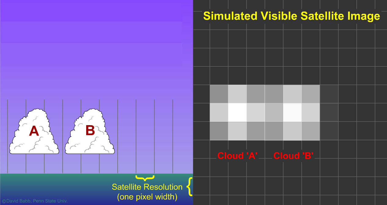
But, when "Cloud B" and "Cloud A" are closer to each other, the simulated satellite image looks quite a bit different. In the image above, "Cloud A" and "Cloud B" are now separated by less than one pixel (parts of each cloud lie in adjacent pixels). The simulated satellite image on the right now shows only one "cloud". So, even though the breadth of each cloud on the simulator is greater than one pixel (they're approximately three pixels wide), we simply can't resolve them as distinct objects at this resolution, because the distance between them is less than the width of one pixel. Make sense?
In a nutshell, satellite resolution is related to the size of the pixels (smaller pixels allow objects to be closer together and still be resolved distinctly). Resolving objects distinctly depends on the distance between objects, not the size of the objects themselves. For example, in the simulated visible satellite image above, the clouds don't look very much like clouds (they look more like white blocks) even though they can be resolved distinctly when there's one pixel between them. The clouds would need to be larger for them to be clearly identified as clouds on the satellite image. The bottom line is that by and large, satellite resolution and the minimum size of an object that allows it to be identified are not the same (although they are related).
To see the impacts of changing image resolution, try the interactive satellite image above (use the slider along the bottom to change resolution). Note that the clouds really begin to look like clouds at 500-meter and 250-meter resolutions, but the various areas of clouds can be resolved distinctly at different stages -- depending on how far apart they are.