Lessons
This is the course outline.
Lesson 1: Getting Started
Overview
Overview
Meteorologists devote their lives to one purpose: to forecast the weather. But many other scientists work to build our understanding of the atmosphere, which is the basis for better prediction that meteorologists can use. Atmospheric science is the foundation upon which all meteorology is based.
Just as with all other physical sciences, mathematics is the language of atmospheric science. If you had our first-year meteorology course, you learned about weather forecasting and some of the physical basis behind the forecasts. This course will introduce you to even more physical concepts of atmospheric science and some of the mathematics that describe and quantify those physical concepts.
You have learned some of the mathematics that you need for this course and will be learning more about vectors and vector calculus soon. In this lesson, we will practice some of the mathematics. You will also prepare an Excel workbook that will help you with some of this course’s assessment problems.
Learning Objectives
By the end of this lesson, you should be able to:
- correctly use significant figures, dimensions, and units
- solve simple problems using integral and differential calculus
- prepare and use a course Excel workbook for course calculations
Questions?
If you have any questions, please post them to the Course Questions discussion forum. I will check that discussion forum daily to respond. While you are there, feel free to post your own responses if you, too, are able to help out a classmate.
1.1 The atmosphere is …
1.1 The atmosphere is …
The atmosphere is amazing, awe-inspiring, frightening, deadly, powerful, boring, strange, beautiful, and uplifting – just a few of thousands of descriptions. So much of our lives depend on the atmosphere, yet we often take it for granted.

Atmospheric science attempts to describe the atmosphere with physical descriptions using words, but also with mathematics. The goal is to be able to write down mathematical equations that capture the atmosphere’s important physical properties (predictability) and to use these equations to determine the atmosphere’s evolution with time (prediction). Predicting the weather has long been a primary focus, but, increasingly, we are interested in predicting climate.
We know quite a lot about the atmosphere. It has taken decades, if not centuries, of careful observation and insightful theory that is based on solid physical and chemical laws. We have more to learn. You could help to advance the understanding of the atmosphere, but you must first understand the physical concepts and mathematics that are already well known. That is a primary purpose of this course – to give you that understanding.
What follows, below, is a series of pictures and graphical images. Each one depicts some atmospheric process that will be covered in this course. Look at these images; you will see them again, each in one of the next ten lessons. Of course, in each observation there are many processes going on simultaneously. In the last lesson, you will have the opportunity to look at an observation and attach the physical principles and the mathematics that describe several processes that are causing the phenomena that you are observing.
Discussion Activity: Finding Errors
We have offered Meteo 300 online many times. However, there may still be errors despite our best efforts.
As we go through the course, if you find an error or typo, post it in the Finding Errors Discussion Forum in Canvas. If you are the first to find an error, you will be awarded 0.1 additional points on your final grade. If you aren't the first one to post, you receive no credit for your find, so it's a good idea to read each lesson at the beginning of each week. A student can earn up to 1 point total (i.e., by being the first to find an error ten times). Now, I hope that we have very few errors, but ...
1.2 You won’t believe what you can do with math!
1.2 You won’t believe what you can do with math!
You’ve been told many times that meteorology is a math-intensive field. It is. But for this course, you already know much of the math, and what you haven’t seen, you will see in vector calculus. To get ready for the meteorology and atmospheric science in this course, you will need to refresh your ability to solve simple math problems, including solving simple problems in differential and integral calculus. At the same time, we will remind you about the importance of correctly specifying significant figures and units in your answers to the problems. The goal of this first lesson is to boost your confidence in the math you already know.
How many figures should be in my answer?
Suppose you are asked to solve the following word problem:
In the radar loop, a squall line is oriented in the north-south direction and is heading northeast at 57 km hr-1. In the last frame of the loop, the line is 17 km west of the Penn State campus. You are out running and know that you can make it back to your apartment in 25 minutes. Will you get back to your apartment before you get soaked?
You reason that the line is moving northeast, and thus, at an angle of 45o relative to the east. Therefore, the eastward motion of the squall line is just the velocity times the cosine of 45o. That gives you the eastward speed. You decide to divide the distance by the eastward speed to get the amount of time before the line hits campus. You plug the numbers into your calculator and get the following result:
According to your calculation, you will make it back with 0.3 minutes (18 seconds) to spare. But can you really be sure that the squall line will strike in 25.3070 minutes? Maybe you should figure out how many significant figures your answer really has. To do that, you need to remember the rules:
Significant Figures Rules
- Non-zero numbers (1,2,3,4,5,6,7,8,9) are ALWAYS significant.
- Zeroes are ALWAYS significant:
- between non-zero numbers
- SIMULTANEOUSLY to the right of the decimal point AND at the end of the number
- to the left of a written decimal point and part of a number 10
- In a calculation involving multiplication or division, multiply numbers as you see them. Then the answer should have the same number of significant figures as the number with the fewest significant figures.
- In a calculation involving addition and subtraction, the number of significant figures in the answer depends on the number of significant figures to the right of the decimal point when all the added or subtracted numbers are put in terms of the same power-of-ten. Add or subtract all the numbers. The answer has the same number of significant figures to the right of the decimal point as the number with the least number of significant figures to the right of the decimal point.
- The number of significant figures is unchanged by trigonometric functions. For other special functions:,
- Logarithms: When taking log of a number with X significant figures, the resulting value should have X number of digits to the right of the decimal point. We can generally apply the same rule for natural logarithms (ln).
- Anti-logarithms: When taking the anti-logarithm (eg. 10value) of a number with X values to the right of the decimal point, the resulting value should have X significant figures. We can generally apply the same rule for exponentials (e).
- Exact numbers never limit the number of significant figures in the result of a calculation and therefore can be considered to have an infinite number of significant figures. Common examples of exact numbers are whole numbers and conversion factors. For example, there are exactly 4 sides to a square and exactly 1000 m in a km.
- For multi-step calculations, any intermediate results should keep at least one extra significant figure to prevent round-off error. Calculators and spreadsheets will typically keep these extra significant figures automatically.
- When rounding, numbers ending with the last digit > 5 are rounded up; numbers ending with the last digit < 5 are rounded down; numbers ending in 5 are rounded up if the preceding digit is odd and down if it is even.
| Number(s) | Answer | Number of Significant Figures | Reason |
|---|---|---|---|
| 25 | 2 | 25 has only 2 significant figures | |
| 8 | 1 | , round to 8 because 0.3 has only 1 significant figure | |
| 2 | , then drop 2 to get | ||
| 2 | , round up then drop 2 to get | ||
| 4.08 | 3 | , trim to 3 significant figures to get 4.08 | |
| 600 | 1 | 200. has 3 significant figures; 200 (no decimal point) has 1 but is ambiguous | |
| 90 | 2 | number in exponent has only 2 significant figures |
Check out this video (11:23): Unit Conversions & Significant Figures for a brief (1 minute) explanation of those rules! Start watching at 9:14 for the most relevant information. Note a minor error starting at 9:50 in which "60" should actually have a decimal point following the zero.
Now to the magic of figuring out how many sig figs your answer should have. There are two simple rules for this. If it's addition or subtraction it's only the number of figures after the decimal point that matters. The number with the fewest figures after the decimal point decides how many figures you can have after the decimal in your answer. So 1,495.2+1.9903 you do the math. First you get 1,497.1903 and then you round to the first decimal, because that first number only had one figure after the decimal. So you get 1,497.2. And for multiplication, just make sure the answer has the same sig figs as your least precise measurement. So 60 x 5.0839 = 305.034, but we only know two sig figs so everything after those first two numbers is zeroes: 300. Of course then we'd have to point out to everyone that the second zero but not the third is significant so we'd write it out with scientific notation: 3.0 * 10^2. Because science! Now I know it feels counterintuitive not to show all of the numbers that you have at your fingertips, but you've got to realize: all of those numbers beyond the number of sig figs you have? They're lies. They're big lying numbers. You don't know those numbers. And if you write them down people will assume that you do know those numbers. And you will have lied to them. And do you know what we do with liars in chemistry? We kill them! Thank you for watching this episode of Crash Course Chemistry. Today you learned some keys to understanding the mathematics of chemistry, and you want to remember this episode in case you get caught up later down the road: How to convert between units is a skill that you'll use even when you're not doing chemistry. Scientific notation will always make you look like you know what you're talking about. Being able to chastise people for using the wrong number of significant digits is basically math's equivalent of being a grammar Nazi. So enjoy these new powers I have bestowed upon you, and we'll see you next time. Crash Course Chemistry was filmed, edited, and directed by Nick Jenkins. This episode was written by me, Michael Aranda is our sound designer, and our graphics team is Thought Bubble. If you have any questions, comments or ideas for us, we are always down in the comments. Thank you for watching Crash Course Chemistry.
What are the typical types of variables?
There are two types of variables – scalars and vectors. Scalars are amount only; vectors also have direction.
Dimensions and units are your friends.
Most variables have dimensions. The ones used in meteorology are:
- L, length
- T, time
- Θ, temperature
- M, mass
- I, electric current
Some constants such as π have no units, but most do.
The numbers associated with most variables have units. The system of units we will use is the International System (SI, from the French Système International), also known as the MKS (meter-kilogram-second) system, even though English units are used in some parts of meteorology.
We will use the following temperature conversions:
We will use the following variables frequently. Note the dimensions of the variables and the MKS units that go with their numbers.
| Type | Variable | Dimensions | MKS Units | Common Unit Name |
|---|---|---|---|---|
| Scalar | length (x or ...) | L | m | |
| area (A) | L2 | m2 | ||
| volume (V) | L3 | m3 | ||
| speed (u, v, w) | L/T | m/s | ||
| energy (E) | ML2/T2 | kg m2/s2 | J = Joule | |
| power (P) | ML2/T3 | kg m2/s3 | W = Watt | |
| density (ρ) | M/L3 | kg/m3 | ||
| pressure (p) | M/LT2 | kg/ms2 | Pa = Pascal | |
| electrical potential | ML2/T3A | kg m2/s3A | V = Volt | |
| temperature (T) | Θ | K | ||
| Vectors | velocity (v) | L/T | m/s | |
| momentum (mv) | ML/T | kg m/s | ||
| acceleration (a) | L/T2 | m/s2 | ||
| force (F) | ML/T2 | kg m/s2 | N = Newton |
Pressure is used for many applications.
p = (normal force)/area = (mass x acceleration)/area = ML/T2L2 = M/LT2
1 Pa = 1 kg m–1 s–2; 1 hPa = 100 Pa = 1 mb = 10–3 bar (hPa = hecto-Pascal)
1013.25 hPa = 1.01325 x 10⁵ Pa = 1 standard atmospheric pressure = 1 atm
Wind speed is another frequently used variable.
The knot (kt) is equal to one nautical mile (approximately one minute of latitude) per hour or exactly 1.852 km/hr. The mile is nominally equal to 5280 ft and has been standardized to be exactly 1,609.344 m.
Thus, 1 m/s = 3.6 km/hr ≈ 1.944 kt and 1 kt ≈ 1.151 mph.
surface winds are typically 10 kts ~ 5 m/s
500 mb winds are ~50 kts ~ 25 m/s
250 mb winds are ~100 kts ~ 50 m/s
Temperature is a third frequently used variable.
Kelvin (K) must be used in all physical and dynamical meteorology calculations. Surface temperature is typically reported in oF (or oC for METARS) and in oC for upper air soundings.
Water vapor mixing ratio is another frequently used variable.
Usually the units for water vapor mixing ratio are g kg-1. In the summer w can be 10 g kg-1; in the winter, it can be 1-2 g kg-1.
Dimensions truly are your friend. Let me give you an example. Suppose you have an equation ax + b = cT, and you know the dimension of b, x (a distance), and T (a temperature), but not a and c. You also know that each term in the equation – the two on the left-hand side and the one on the right-hand side – must all have the same units. Therefore, if you know b, you know that the dimensions of a must be the same as the dimensions of b divided by L (length) and the dimensions of c must be the same as the dimensions of b divided by Θ.
Also, if you invert a messy equation and you're not sure that you didn’t make a mistake, you can check the dimensions of the individual terms and if they don’t match up, it’s time to look for your mistake. Or, if you have variables multiplied or divided in an exponential or a logarithm, the resulting product must have no units.
So, how do you find the dimensions of units of an integral equation? One way to look at this problem is the figure out the dimension or the units of the integral's solution. Or, if you do not want to solve the integral, then you just assign the dimensions or units of each term in the integral expression, even the differentials such as dx, dt. The integrals symbols themselves have no dimensions or units. For example, take the integral of force over a distance, which is the integral of F dx. Pay no attention to the integral symbol. The dimensions of F are MLT-2 and the dimensions of dx are L, so when you multiply them together, you get MLT-2 *L = ML2 T-2, which has the same units as energy!
To find the dimensions or units of a derivative, the same thought process should be applied: either figure out the dimensions or units that the actual derivative would have, or if you do not want to solve the derivative, assign dimensions or units to every term in the equation that can have dimensions and units. For example, in dx/dt, dx is just a length and dt is just a time, so assign them those dimensions or units, which in this example is L/T or m/s. On the other hand, d/dt by itself has just the dimension of 1/T because the expression "d" has no units by itself. You now see that finding the dimensions or units for integral or derivative expressions is just as easy as for algebraic expressions.
Always write units down and always check dimensions if you aren’t sure. That way, you won’t crash your spacecraft on the back side of Mars [3]. View the following video (2:42).
Remember when NASA lost a spacecraft because it's simultaneously used Imperial and metric measurements on the same mission? The Mars Climate Orbiter disappeared 15 years ago this month and here's a very brief recap of exactly what went wrong. The Mars Climate Orbiter launched on December 11, 1998 on a mission to orbit Mars. This first interplanetary weather satellite was designed to gather data on Mars' climate and also serve as a relay station for the Mars Polar Lander, a mission that launched a few weeks later. But you can't just launched a spacecraft towards Mars and trust that it's going to get where it's going. You to have to monitor its progress. Many spacecraft have reaction wheels to keep them oriented properly and navigation teams behind interplanetary spacecraft that constantly monitor the angular momentum and adjust trajectory to make sure it gets exactly where it needs to go. In the case of the Mars Climate Orbiter, monitoring its trajectory and angular momentum involved a few steps. First, data from the spacecraft was transferred to the ground by telemetry. There it was processed by a software program and stored in an angular momentum desaturation file that process data was what scientists used to adjust the trajectory. Adjustments that were made by firing the spacecraft's thrusters. Every time the thrusters were fired, the resulting change in velocity was measured twice: once by software program on the spacecraft and once by software program off the ground. And here's where the problem comes in. It turned out that the two systems the processing software on the spacecraft and the software on the ground we're using two different units of measurements. The software on the spacecraft measured impulse, or the changes by thrusters in newton seconds a commonly accepted metric unit of measurement, while the processing software on the ground use the Imperial pound seconds. And it was unfortunately the ground computer's data that scientists used to update the spacecraft trajectory and because one pound of force is equal to 4.45 Newton's every adjustment was off by a factor of 4.45. For a spacecraft traveling tens of millions of miles to destination a number of seemingly small errors really add up. During the Mars Climate Orbiters nine-month cruise to Mars seven errors were introduced into its trajectory that meant that when it reached the red planet it was 105 miles closer to the Martian surface than expected. This turned out to be an unsurvivably low altitude for its Mars encounter when the spacecraft fire its main engine for the orbit insertion burn that was designed to put it into an elliptical orbit nothing happened. NASA lost contact quite abruptly with the spacecraft. So while we know the root cause of just what went wrong we'll never know exactly what happened to the Mars Climate Orbiter. The loss of the Mars Climate Orbiter very sadly happened in space. Leave your spacey questions and comments below, and don't forget to subscribe.
Quiz 1-1: Significant figures, dimensions, and units.
Now it's time to to take a quiz. I highly recommend that you begin by taking the Practice Quiz before completing the graded Quiz. Practice Quizzes are not graded and do not affect your grade in any way–except to make you more competent and confident to take the graded Quizzes : ).
- In Canvas, find Practice Quiz 1-1. You may complete this practice quiz as many times as you want. It is not graded, but it allows you to check your level of preparedness before taking the graded quiz.
- When you feel you are ready, take Quiz 1-1. You will be allowed to take this quiz only once. This quiz is timed, so after you start, you will have a limited amount of time to complete it and submit it. Good luck!
1.3 If you thought practice makes perfect, you could be right.
1.3 If you thought practice makes perfect, you could be right.
Calculus is an integral part of a meteorologist’s training. The ability to solve problems with calculus differentiates meteorologists from weather readers. You should know how to perform both indefinite and definite integrals. Brush up on the derivatives for variables raised to powers, logarithms, and exponentials. We will take many derivatives with respect to time and to distance.
Need Extra Practice?
Visit the Khan Academy website that explains calculus with lots of examples [5], practice problems, and videos. You can start with single variable calculus, but may find it useful for more complicated calculus problems.
Simple Integrals and Derivatives That are Frequently Used to Describe the Behavior of Atmospheric Phenomena
1.
2.
3.
4.
5.
You have the power.
Often in meteorology and atmospheric science you will need to manipulate equations that have variables raised to powers. Sometimes, you will need to multiply variables at different powers together and then rearrange your answer to simplify it and make it more useful. In addition, it is very likely that you will need to invert an expression to solve for a variable. The following rules should remind you about powers of variables.
Laws of Exponents
If , then raise both sides to the exponent to move the exponent to the other side:
If , and you want to get an equation with a raised to no power, then raise both sides to the exponent :
This brief video (7:42) sums up these important rules:
In this video we're going to be talking about all of the basic rules of exponents. And remember, when we're talking about exponents we can have an exponent here like X to the fourth where x is the base what we call the base and four is the exponent this small number in the upper right hand corner. It means that we're going to multiply X by itself four times or it means we have four factors of X multiplied together. So, if we expand this out its x times X times X times X. if we collapse it its X to the fourth. So, what happens when we do addition, subtraction, multiplication, and division of exponents? Well, in all cases we have to be really careful about like terms. For example, when we add terms that have exponents in them together both the bases and the exponents have to be the same in order for us to add them together. So, if we look at this first example 3x squared plus 2x squared the base here is X and the base here is X so the bases are the same which is good because we need that. and the exponents we have 2 and 2 which is good because we also need the exponents to be the same in order to add these together. So basically we have 3x squared added to 2x squared is going to give us five of them, 5x squared. So, if you're going to do addition and subtraction the bases and the exponents have to be the same. In this case we have X to the third plus x squared our bases X are the same but our exponents are different we have three and two. These are not like terms, so we can't add these together we can't simplify this at all. What happens when we do subtraction well again we're looking for similar basis so we have X and X for our base and then we have exponents of four and four. So because the bases and the exponents of the scene we can combine these like terms. We have six of them were subtracting and applied one of them which is going to leave us with five of them. So 5 times X to the fourth, but in this problem despite having the same base they will have a base of X we have different exponents we have a 4 and a 3 and because we're doing subtraction we can't combine these. We can't simplify this at all. What happens when we multiply two values together where exponents are involved? Well, here in order to simplify all we care about is that the bases are the same. The exponents do not have to be the same. So here we have base X and base X and we know already that's all we need to multiply these together it doesn't matter that the exponents are also the same we just add them. So we have three times to these are coefficients on our x squared terms. We multiply those together. So three times two is six, so that's going to be the first part and then we have x squared times x squared. And if we look at that x squared times x squared what we're going to do is add the exponents together. And the reason is because if we expand these out we know that x squared is two factors of X multiplied together. We're multiplying that by another x squared, so we're multiplying that by two more factors of X multiplied together. All together this is X to the fourth. Which we know because this essentially becomes the rule x to the a x x to the B is X to the a plus B. We just add the exponents together. So two plus two is four we get X to the fourth. Here's another example we have X to the third times x squared remember there's an implied one coefficient in front of both of these when we multiply 1 x 1 we get one so there will be a implied one coefficient on our final answer. x cubed + x squared. We just care that the bases are the same and they both have a base X so we know will be able to multiply them together. We have X to the third times x squared and remember that is going to be X to the three plus two so when we simplify we get X to the fifth and that should make sense because we have 3 factors of x x 2 factors of X adding them all up we get five factors of X so X to the fifth. The quotient rule for exponents tells us that in the same way as when we multiplied we didn't have to have the same exponent. When we divide we also don't have to have the same exponent we only care about the bases so here we have like basis. We have base X for both of these the exponents happened to be the same but that doesn't matter we're just going to leave this six and our final answer, so we'll get six here. And then what we're going to do is subtract the exponent in the denominator from the exponent in the numerator so the result is going to be X to the 4 minus 4. This is the four from the numerator this is the four from the denominator. 4-4 is 0 so we get 6 x 20 x to the 0 is 1 so this is 6 times 1 or just six. Even if we have different numbers again we only care about the bases both of these have the same base of X so again we'll just keep our two and our final answer and then we'll have X to the 4-3 because we say numerator exponent minus denominator exponent. That's going to give us 2 times X to the 4 minus 3 is 1. so X to the first which is of course just equal to 2x. What about a power raised to another power or an exponent raised to another exponent? Well, just like before in this example here when we said X to the fourth means multiply X by itself four times here we're saying multiply x squared by itself three times. So this is going to be equal to x squared times x squared times x squared and now we're really just back at this right here for multiplying like bases together and we add the exponents. So, this is just the same as X to the two plus two plus two. Two plus two plus two is six so we get x to the sixth power. What we realize then is that we can expand this and then add the exponents together using this rule over here or we can just multiply these two exponents together. Two times three gives us six and so we can do it that way as well. We can even do this when we have a negative base. So this problem here is telling us multiply 3 factors of negative x squared together so this is going to be negative x squared times negative x squared times negative x squared. We can deal with the negatives separately. Remember we can cancel every two negatives and they become a positive so negative and negative become a positive we're just left with this single negative sign here. so our answer will be negative and then x squared times x squared times x squared we know is X to the sixth. You can also think about it this way when you have this negative sign inside the parentheses. It's the same thing as saying negative 1 times x squared all raised to the third power and then you can apply this exponent to the negative 1 negative 1 times negative 1 times negative 1 is going to give you negative 1 which is this part right here. And then x squared to the third is going to be X to the 60 you get this X to the sixth and when you multiply them together you get negative x to the sixth. So those are just some of the most basic exponent rules that you need to know.
Are you ready to give it a try? Solve the following problem on your own. After arriving at your own answer, click on the link to check your work. Here we go:
Check Your Understanding
What does y equal?
Quiz 1-2: Solving integrals and differentials.
Now it's time to to take another quiz. Again, I highly recommend that you begin by taking the Practice Quiz before completing the graded Quiz, since it will make you more competent and confident to take the graded Quiz : ).
- Go to Canvas and find Practice Quiz 1-2. You may complete this practice quiz as many times as you want. It is not graded, but it allows you to check your level of preparedness before taking the graded quiz.
- When you feel you are ready, take Quiz 1-2. You will be allowed to take this quiz only once. This quiz is timed, so after you start, you will have a limited amount of time to complete it and submit it. Good luck!
1.4 Are you ready to get with the programming?
1.4 Are you ready to get with the programming?
Meteorologists and atmospheric scientists spend much of their time thinking deep thoughts about the atmosphere, the weather, and weather forecasts. But to really figure out what is happening, they all have to dig into data, solve simple relationships they uncover, and develop new ways to look at the data. Much of this work is now done by programming a computer. Many of you haven’t done any computer programming yet, and for those of you who have, congratulations – put it to good use in this class. For those who are programming novices, we can introduce you to a few of the concepts of programming by getting you to use Excel or another similar spreadsheet program.
To help you learn and retain the concepts and skills that you will learn in this course, you will solve many word problems and simple math problems. For several activities, we give you the opportunity to practice solving particular types of problems enough times until you gain confidence that you can solve those same types of problems on a quiz. That means that you will be solving some types of problems several times and only the numbers for the variables will change. The simplest way for you to solve these problems is to program a spreadsheet to do that repetitive math for you.

Screenshot shows an Excel Spreadsheet
A text box says "put activity number in row 1" and an arrow points to cell A1.
A second text box says "put variable names in row 2" with an arrow pointing to cells A2 and B2
A third text box says "start numbers for variables in row 3" with an arrow pointing to cells A3 and B3
A final text box says "calculations follow variable numbers" with an arrow pointing to C3.
Let’s do a simple example. Suppose we have several boxes, some with different shapes and sizes, and we want to calculate the volume of the boxes and find the total volume. I have put in the names of the variables (with units!) and then the numbers for the length, width, and height of each box type and the total number of each box. To calculate the volume of each box, click on E3 and put an “= a3*b3*c3” in the equation line. Hit enter and it will do the calculation and put the answer in E3. A small square will appear in the lower right corner of E3. Click on this square with the mouse and pull down over the next three rows. Excel will automatically do the calculations for those rows. To calculate the total volume, go to F3 and enter “=d3*e3,” and hit “enter.” Grab the small box and pull down to get the total volume of each type of box. To get the total volume, click on F7, click on “Formulas,” and then “AutoSum,” and finally “Sum.” Excel will show you which cells it intends to sum. You can change this by adjusting the edges of the box it shows. Finally, pay attention to significant digits in your calculated volumes. You can adjust the number of decimal places by highlighting a cell or group of cells and then by clicking on the appropriate icon on the Excel tool bar. Note that an incorrect number of significant figures is displayed in some of the answers--see if you can figure out where.

| length (m) | width (m) | height (m) | number of boxes | box volume (m3) | total volume (m3) |
|---|---|---|---|---|---|
| 0.72 | 0.52 | 0.52 | 3 | =A3*B3*C3 | |
| 0.52 | 0.52 | 0.52 | 4 | ||
| 1.2 | 0.85 | 1.01 | 1 | ||
| 0.62 | 0.62 | 0.95 | 2 |

| length (m) | width (m) | height (m) | number of boxes | box volume (m3) | total volume (m3) |
|---|---|---|---|---|---|
| 0.72 | 0.52 | 0.52 | 3 | 0.19 | 0.58 |
| 0.52 | 0.52 | 0.52 | 4 | 0.14 | 0.56 |
| 1.2 | 0.85 | 1.01 | 1 | 1.03 | 1.03 |
| 0.62 | 0.62 | 0.95 | 2 | 0.37 | 0.73 |
Hopefully this example is a refresher for most of you. For those who are totally unfamiliar with Excel, please click on the question mark in the upper right of the screen and type in the box “creating your first workbook.” You can also visit Microsoft's help page for additional step-by-step instructions for how to Use Excel as Your Calculator [9]. The best way to learn, after the introduction, is by doing. The Keynote Support website [10] also lists helpful summaries of instructions.
Activity 1-3: Setting up your Meteo 300 Excel workbook.
Please follow the instructions above for setting up an Excel workbook. You will be using this workbook to do calculations, plot graphs, and answer questions on quizzes and problems for the rest of the course.
Use the same headings and the same numbers in the first four columns. Enter your own equations and find the box volumes and total volumes.
This assignment is worth 15 points. Your grade will mostly depend upon showing that you set up the workbook, but some additional points will be assigned contingent upon how well you follow the instructions. When your Excel workbook is complete, please do the following:
- Make sure that the file for your workbook follows this naming convention: Workbook_your last name (i.e., Smith)_your first name_(i.e., Eileen).xlsx.
- In Canvas, find Activity 1-3: Setting up your Meteo 300 Excel workbook. Upload your Excel workbook there.
Summary and Final Tasks
Summary
There is a very good reason that you are taking this class and I am teaching it – all of us are fascinated by the weather, awed by the atmosphere’s power, and passionate about learning more about it. Quite honestly, I can’t imagine a more rewarding career than the one that you are embarking upon or the one that I have. Nothing could be more rewarding than saving lives by making the atmosphere more predictable or by making the perfect prediction. Nothing.
But, do you know what? The best forecasters are the ones who can not only read weather maps, but who also know physically what the atmosphere is doing. The best forecasters know how to translate the physics into mathematics so that hand-waving can be turned into usable numbers. This course will start to make all of these connections between observations and physical cause-and-effect and help us find numerical solutions to questions.
For those of you who are in related disciplines, this course will give you a solid basic understanding of the atmosphere that you can apply in your studies and career, whether it be civil engineering, mechanical engineering, environmental engineering, chemistry, hydrology, or many other fields.
We have now reviewed some important concepts like significant figures and dimensions and units. You will continue to gain confidence in using the differential and integral calculus that you already know. As you go through the course, I want you to look back at the pictures of the atmosphere and imagine which equations are governing the processes that are causing your observations.
Reminder - Complete all of the Lesson 1 tasks!
You have reached the end of Lesson 1! Make sure that you have completed all of the tasks in Canvas.
Lesson 2: Thermodynamics
Overview
Overview
The atmosphere is composed of billions of billions of molecules, 1043 molecules to be exact. Each molecule is zooming at hundreds of meters per second but colliding with other molecules each billionth of a second, exchanging kinetic energy (½ mv2), momentum (mv), and internal energy (rotations and vibrations). It’s impossible to calculate what all of these molecules will do, so instead we study the energy and energy changes of volumes of molecules and use this information in our forecast models. This study is called thermodynamics. Thermodynamics has some difficult concepts to master, but it is also part of your everyday experience. In this lesson, you will learn the fundamental laws of thermodynamics and see how they describe our atmosphere’s pressure and temperature structure. You will learn why the atmosphere is sometimes stable and what happens when it isn’t.
Learning Objectives
By the end of this lesson, you should be able to:
- use the fundamental gas laws - Ideal Gas Law, Dalton’s Law – to determine the relative densities of different air masses
- derive the hydrostatic equilibrium equation from force balance to show why atmospheric pressure decreases with height
- use the 1st Law of Thermodynamics and conservation of energy (i.e., adiabatic processes) to explain air parcel temperature changes
- determine stability for different dry environmental temperature profiles
- calculate buoyancy and vertical velocity with time
Questions?
If you have any questions, please post them to the Course Questions discussion forum. I will check that discussion forum daily to respond. While you are there, feel free to post your own responses if you, too, are able to help out a classmate.
2.1 Gas Laws
2.1 Gas Laws
Understanding atmospheric thermodynamics begins with the gas laws that you learned in chemistry. Because these laws are so important, we will review them again here and put them in forms that are particularly useful for atmospheric science. You will want to memorize these laws because they will be used again and again in many other areas of atmospheric science, including cloud physics, atmospheric structure, dynamics, radiation, boundary layer, and even forecasting.
Looking Ahead
Before you begin this lesson's reading, I would like to remind you of the discussion activity for this lesson. This week's discussion activity will ask you to take what you learn throughout the lesson to answer an atmospheric problem. You will not need to post your discussion response until you have read the whole lesson, but keep the question in mind as you read:
This week's topic is a hypothetical question involving stability. The troposphere always has a capping temperature inversion—it's called the stratosphere. The tropopause is about 16 km high in the tropics and lowers to about 10 km at high latitudes. The stratosphere exists because solar ultraviolet light makes ozone and then a few percent of the solar radiation is absorbed by stratospheric ozone, heating the air and causing the inversion. Suppose that there was no ozone layer and hence no stratosphere caused by solar UV heating of ozone.
Would storms in the troposphere be different if there was no stratosphere to act like a capping inversion? And if so, how?
You will use what you have learned in this lesson about the atmosphere's pressure structure and stability to help you to think about this problem and to formulate your answer and discussions. So, think about this question as you read through the lesson. You'll have a chance to submit your response in 2.6!
Ideal Gas Law
The atmosphere is a mixture of gases that can be compressed or expanded in a way that obeys the Ideal Gas Law:
where p is pressure (Pa = kg m–1 s–2), V is the volume (m3), N is the number of moles, R* is the gas constant (8.314 J K–1 mole–1), and T is the temperature (K). Note also that both sides of the Ideal Gas Law equation have the dimension of energy (J = kg m2 s–2).
Recall that a mole is 6.02 x 10²³ molecules (Avogadro’s Number). Equation 2.1 is a form of the ideal gas law that is independent of the type of molecule or mixture of molecules. A mole is a mole no matter its type. The video below (6:17) provides a brief review of the Ideal Gas Law. Note that the notation in the video differs slightly from our notation by using n for N, P for p, and R for R*.
So here I have a tank filled with gas. And these little dots represent some of the gas particles that would be in this tank. The arrows I put in here because all of these particles are in constant random motion. They're like a bunch of hyperactive little kids, running into each other all the time, banging into the sides of the container, and so forth. So we've got this tank of gas. Let's think about the characteristics that we could use to describe it. So one of the things that we could do is we could say what its temperature is. The higher the temperature, remember, the faster these gas particles are moving around, so temperature is very important when we talk about gas. Temperature for gases should always be reported in Kelvin. So we could say, for example, that the temperature of this guy here is 313 Kelvin. That's how hot these gas particles in the sample are. When you talk about gas, another important characteristic is pressure. How hard are these gas particles bouncing against the sides of the tank? How much pressure are they exerting on them? And we could measure these with a pressure gauge or something like that on the top of this tank. We could say, the pressure for this is 3.18 atm. That might be a pressure. And another thing that we spend a lot of time talking about when it comes to gas is volume. And again, I have these letters here that are how each one of these things are abbreviated. Volume, V, volume of this tank might be something like 95.2 liters. And finally, look at these particles that I've drawn. There is a certain amount of gas that's in here. And the amount of gas, which is abbreviated by the little letter n, is usually reported in moles, which is a convenient measure of how much of something we have. So we could say that the amount of gas in this tank is 7.5 moles. Now, whenever we have a sample of gas like this, if it's a tank or it's in a balloon or wherever it is, we can describe-- we can give it these various characteristics. And it turns out that also, for any sample of gas, if we know three of these characteristics, we can figure out what the fourth is. All we need to do is know three. And in order to do that, we use an equation that's a representation of the Ideal Gas Law. And it's written as P times V, pressure times volume, equals n, the amount of gas, times R times T, temperature. I'll get to R in a second. Don't worry about it for right now. It's going to be a number that we know. So let's say, for example, that we didn't know what pressure was, but we still knew the temperature, volume, and the amount of gas. No big deal. We could take the equation, PV equals nRT, and rearrange it. Divide both sides by V. Get rid of the V. And then we'd have P equals nRT divided by V. Plug these values in, and we could figure out what the pressure was. Or let's say that we knew what the pressure was of a particular gas sample. We know what the temperature was in a volume. But we didn't know what the amount of gas was. We don't know how much we had. We could figure out that fourth characteristic by rearranging the Ideal Gas Law for n, canceling out R and T on one side, rearranging it to solve for n. And then we could plug in the pressure, the volume, and the temperature, and we could figure out the amount of gas. So in other words, if we know three of these characteristics, we can always figure out what the fourth is. So you may be asking yourself, so R-- what's R? R is what we call a constant. It's a number that we know ahead of time that doesn't depend on the variables in our problem. The R that I'm going to be using most of the time for the videos is 0.0821 liters times atm divided by Kelvin times moles. Now notice that this is a fraction. It has both a top and a bottom. And it also is not just a number, but it has units. And check this out-- the units on R match the units in my problem. They match the characteristics that I'd be using. So I have liters here, liters here, atm, atm, Kelvin, Kelvin, and moles, moles. You always want the units on R to match the units of the characteristics in your Ideal Gas Problem. So because you always want the units to match, there are also different values of R, although I'm going to be using this mostly for the videos I'm doing. For example, let's say that instead of atm, I was using a pressure that was in millimeters of mercury. In this case, I wouldn't want to use this R here. I'd want to use this R here, so that the units match-- millimeters of mercury here, millimeters of mercury here, and the number's different-- 62.4. So again, that's what I use here. Let's say that instead of millimeters of mercury, my pressure was given to me in kPa. I would then use this value of R so that the units match. I've got kPa here, kPa here, and all the others are the same, so 8.31 for that. Now as I keep saying, in most of the videos that I'm going to be doing, I'm going to be using this top R with atm. But you may be asked by your teacher to use a different R. It's no big deal. That's probably just because they're giving you problems that have different pressure units, and they want the pressure units to match. So don't worry at all if you're using one of these other R's. Setting up and solving the Ideal Gas Law is exactly the same. No matter which of these R's you use, it's just a matter of plugging a different R in at the very end. So no matter which one you're using, you should be able to follow all these lessons, and it should all make sense.
Usually in the atmosphere we do not know the exact volume of an air parcel or air mass. To solve this problem, we can rewrite the Ideal Gas Law in a different useful form if we divide N by V and then multiply by the average mass per mole of air to get the mass density:
where M is the molar mass (kg mol–1). Density has SI units of kg m–3. The Greek symbol ρ (rho) is used for density and should not be confused with the symbol for pressure, p.
Thus we can put density in the Ideal Gas Law:
Density is an incredibly important quantity in meteorology. Air that is more dense than its surroundings (often called its environment) sinks, while air that is less dense than its surroundings rises. Note that density depends on temperature, pressure, and the average molar mass of the air parcel. The average molar mass depends on the atmospheric composition and is just the sum of the mole fraction of each type of molecule times the molar mass of each molecular constituent:
where the i subscript represents atmospheric components, N is the number of moles, M is the molar mass, and f is the mole fraction. This video (3:19) shows you how to find the gas density using the Ideal Gas Law. You will note that the person uses pressure in kPa and molar mass in g/mol. Since kPa = 1000 Pa and g = 1/1000 kg, the two factors of 1000 cancel when he multiplies them together and he can get away with using these units. I recommend always converting to SI units to avoid confusion. Also, note that the symbol for density used in the video is d, which is different from what we have used (ρ, the convention in atmospheric science).
Hey guys how do you solve ideal gas law questions involving density? The key is to have a formula or know how to derive the formula on your own. Remember density is mass over volume. Now, the way that mass is found in the ideal gas law equation is in n because the number of moles is the same as mass over molar mass. So, check this set. I'm going to replace n with mass over molar mass, and then I'm going to rearrange for m over v. I'm going to undo division by molar mass on the other side and then I'm going to undo multiplication by RT and bring my V over. Here's a what I mean. P times the molar mass divided by RT gives me mass over volume. Mass over volume is density and so my equation is density equals pressure times molar mass divided by RT. We can now use this equation to find the density of oxygen at 55 Celsius and a hundred and three kilopascals. So let's do it. The density is pressure that's 103 kilopascals times molar mass for oxygen. That's 32 grams per mole. R, now, I'm going to put my volume in liters and I'm going to put my pressure in kilopascals which means the relevant are that I want is 8.314 liters, kilopascals per mole Kelvin and my temperature in Kelvin is the temperature in Celsius plus 273, which gives me 328 Kelvin. And all of these units should cancel out to give me a density unit. Kelvin cancels of Kelvin per moles cancel / moles kilopascals canceled the scale pascals and left with grams per liter. Let's do this on the calculator 103 times 32 divided 8.314 divided 328. That's 1.21 grams per liter. That may not seem like a lot, but remember you're dealing with the gas here. If you have a 1-liter balloon how much is it actually going to weigh? Probably the amount of the rubber plus like a gram or so. This here is the density of oxygen gas at 55 and 103 kilopascals. This is your density formula in terms of the ideal gas law. Be able to use it. Best of luck!
Solve the following problem on your own. After arriving at your own answer, click on the link to check your work.
Example
Let’s calculate the density of dry air where you live. We will use the Ideal Gas Law and account for the three most abundant gases in the atmosphere: nitrogen, oxygen, and argon. The mole fractions of the gases are 0.78, 0.21, and 0.01, respectively. M is the molar mass of air; M = 0.029 kg mol–1, which is just an average that accounts for the mole fractions of the three gases:
R* = 8.314 J K–1 mol–1. Here, p = 960 hPa = 9.6 x 10⁴ Pa and T = 20 oC = 293 K.
Putting these values into the equation 2.3, we get that the dry air density is 1.1 kg m–3.
What would the density be if the room were filled with helium and not dry air at the same pressure and temperature?
Helium density = (pressure times molar mass of helium)/(Ideal Gas Law constant in SI units times temperature in K) = 0.16 kg m–3
Dry Air
Often in meteorology we use mass-specific gas laws so that we must specify the gas that we are talking about, usually only dry air (N2 + O2 + Ar + CO2 +…) or water vapor (gaseous H2O). We can divide R* by Mi to get a mass-specific gas constant, such as Rd = R*/Mdry air.
Thus, we will use the following form of the Ideal Gas Law for dry air:
where:
.
Mdry air is 0.02897 kg mol–1, which is the average of the molar masses of the gases in a dry atmosphere computed to four significant figures.
Note that p must be in Pascals (Pa), which is 1/100th of a mb (a.k.a, hPa), and T must be in Kelvin (K).
Water Vapor
We can do the same procedure for water vapor:
where .
Typically e is used to denote the water vapor pressure, which is also called the water vapor partial pressure.
Dalton’s Law

This gas law is used often in meteorology. Applied to the atmosphere, it says that the total pressure is the sum of the partial pressures for dry air and water vapor:
Imagine that we put moist air and an absorbent in a jar and screw the lid on the jar. If we keep the temperature constant as the absorbent pulls water vapor out of the air, the pressure inside the jar will drop to pd. Always keep in mind that when we measure pressure in the atmosphere, we are measuring the total pressure, which includes the partial pressures of dry air and water vapor.
So it follows that the density of dry air and water vapor also add:
Check Your Understanding
Suppose we have two air parcels that are the same size and have the same pressure and temperature, but one is dry and the other is moist air. Which one is less dense?
We can solve this one without knowing the pressure, temperature, or volume. Let’s assume that 98% of the molecules are dry air, which means the remaining 2% are dry air in the first case and water vapor in second case. Dry air is 0.029 kg mol–1 and water vapor is 0.018 kg mol–1, so 2% of the moist air is lighter than the 2% of dry air, and when we consider the total air, this means that for the same temperature and pressure, moist air is always less dense than dry air.
Virtual Temperature
Suppose there are two air parcels with different temperatures and water vapor amounts but the same pressure. Which one has a lower density? We can calculate the density to determine which one is lighter, but there is another way to do this comparison. Virtual temperature, Tv, is defined as the temperature dry air must have so that its density equals that of ambient moist air. Thus, virtual temperature is a property of the ambient moist air. Because the air density depends on the amount of moisture (for the same pressure and temperature), we have a hard time determining if the air parcel is more or less dense relative to its surroundings, which may have a different temperature and amount of water vapor. It is useful to pretend that the moist parcel is a dry parcel and to account for the difference in density by determining the temperature that the dry parcel would need to have in order to have the same density as the moist air parcel.
We can define the amount of moisture in the air by a quantity called specific humidity, q:
We see that q is just the fraction of water vapor density relative to the total moist air density. Usually q is given in units of g of water vapor per kg of dry air, or g kg–1.
Using the Ideal Gas Law and Dalton’s Law, we can derive the equation for virtual temperature:
where T and Tv have units of Kelvin (not oC and certainly not oF!) and q must be unitless (e.g., kg kg–1).
Note that moist air always has a higher virtual temperature than dry air that has the same temperature as the moist air because, as noted above, moist air is always less dense than dry air for the same temperature and pressure. Note also that for dry air, q = 0 and the virtual temperature is the same as the temperature.
Solve the following problem on your own. After arriving at your own answer, click on the link to check your work.
Check Your Understanding
Consider a blob of air (Tblob = 25 oC, qblob = 10 g kg–1) at the same pressure level as a surrounding environment (Tenv = 26 oC and qenv = 1 g kg–1). If the blob has a lower density than its environment, then it will rise. Does it rise?
We will use equation 2.10. Remember to convert T from oC to K and q from g kg–1 to kg kg–1!
We see that the blob is less dense than its environment and so will rise. This difference of 0.6 oC may seem small, but it makes a huge difference in upward motion.
The following are some mistakes that are commonly made in the above calculations:
- not converting from oC to K:
We calculate that Tvblob < Tvenv, which is the wrong answer.
- not converting q from g/kg to kg/kg:
We calculate that Tvblob > Tvenv, which is correct in this case, but the numbers are crazy! After you complete your calculations, if the numbers you get just don’t seem right—like these—then you know that you have made a mistake in the calculation. Go looking for the mistake. Don’t submit an answer that makes no sense.
Once we find Tv, we can easily find the density of a moist parcel by using equation 2.5, in which we substitute Tv for T. Thus,
Quiz 2-1: What will that air parcel do?
This quiz will give you practice calculating the virtual temperature and density using the Excel workbook that you set up in the last lesson.
- Go to Canvas and find Practice Quiz 2-1. You may complete this practice quiz as many times as you want. It is not graded, but it allows you to check your level of preparedness before taking the graded quiz. I strongly suggest that you enter the equations for density and for virtual temperature in your Excel worksheet and use them to do all your calculations of density and virtual temperature on both the practice quiz and the quiz.
- When you feel you are ready, take Quiz 2-1. You will be allowed to take this quiz only once. This quiz is timed, so after you start, you will have a limited amount of time to complete it and submit it. Good luck!
2.2 The Atmosphere’s Pressure Structure: Hydrostatic Equilibrium
2.2 The Atmosphere’s Pressure Structure: Hydrostatic Equilibrium
The atmosphere’s vertical pressure structure plays a critical role in weather and climate. We all know that pressure decreases with height, but do you know why?

The atmosphere’s basic pressure structure is determined by the hydrostatic balance of forces [17]. To a good approximation, every air parcel is acted on by three forces that are in balance, leading to no net force. Since they are in balance for any air parcel, the air can be assumed to be static or moving at a constant velocity.
There are 3 forces that determine hydrostatic balance:
- One force is downwards (negative) onto the top of the cuboid from the pressure, p, of the fluid above it. It is, from the definition of pressure [18],
[2.11]
- Similarly, the force on the volume element from the pressure of the fluid below pushing upwards (positive) is:
[2.12]
- Finally, the weight [19] of the volume element causes a force downwards. If the density [20] is ρ, the volume is V, which is simply the horizontal area A times the vertical height, Δz, and g the standard gravity [21], then:
[2.13]
By balancing these forces, the total force on the fluid is:
This sum equals zero if the air's velocity is constant or zero. Dividing by A,
or:
Ptop − Pbottom is a change in pressure, and Δz is the height of the volume element – a change in the distance above the ground. By saying these changes are infinitesimally [22] small, the equation can be written in differential [23] form, where dp is top pressure minus bottom pressure just as dz is top altitude minus bottom altitude.
The result is the equation:
This equation is called the Hydrostatic Equation. See the video below (1:18) for further explanation:
Consider an air parcel at rest. There are three forces in balance, the downward pressure force, which is pressure times area in the parcel's top, and an upward pressure force on the parcel's bottom, and the downward force of gravity actually on the parcel's mass, which is just the acceleration due to gravity times the parcel's density times it's volume. The volume equals the parcel's cross sectional area times its height. We can sum these three forces together and set them equal to 0 since the parcel's at rest. Notice how the cross sectional area can be divided out. The next step is to put the pressure difference on the left hand side. And then shrink the air parcel height to be infinitesimally small, which makes the pressure difference infinitesimally small. By dividing both sides by the infinitesimally small height, we end up with an equation that's the derivative of the pressure with respect to height, which is equal to minus the parcel's density times gravity. This equation is the hydrostatic equation, which describes a change of atmospheric pressure with height.
Using the Ideal Gas Law, we can replace ρ and get the equation for dry air:
We could integrate both sides to get the altitude dependence of p, but we can only do that if T is constant with height. It is not, but it does not vary by more than about ±20%. So, doing the integral,
H is called a scale height because when z = H, we have p = poe–1. If we use an average T of 250 K, with Mair = 0.029 kg mol–1, then H = 7.3 km. The pressure at this height is about 360 hPa, close to the 300 mb surface that you have seen on the weather maps. Of course the forces are not always in hydrostatic balance and the pressure depends on temperature, thus the pressure changes from one location to another on a constant height surface.
From equation 2.20, the atmospheric pressure falls off exponentially with height at a rate given by the scale height. Thus, for every 7 km increase in altitude, the pressure drops by about 2/3. At 40 km, the pressure is only a few tenths of a percent of the surface pressure. Similarly, the concentration of molecules is only a few tenths of a percent, and since molecules scatter sunlight, you can see in the picture below that the scattering is much greater near Earth's surface than it is high in the atmosphere.

Quiz 2-2: Harnessing the power of the hydrostatic equation
This quiz will give you practice using the hydrostatic equation to learn interesting and useful properties and quantities of the atmosphere.
- I strongly suggest that you do all your calculations on this quiz using the Excel workbook.
- There is no Practice Quiz 2-2. However, you have extra time to take this quiz.
- When you feel you are ready, take Quiz 2-2 in Canvas. You will be allowed to take this quiz only once. This quiz is timed, so after you start, you will have a limited amount of time to complete it and submit it. Good luck!
2.3 First Law of Thermodynamics
2.3 First Law of Thermodynamics
Weather involves heating and cooling, rising air parcels and falling rain, thunderstorms and snow, freezing and thawing. All of this weather occurs according to the three laws of Thermodynamics. The First Law of Thermodynamics tells us how to account for energy in any molecular system, including the atmosphere. As we will see, the concept of temperature is tightly tied to the concept of energy, namely thermal energy, but they are not the same because there are other forms of energy that can be exchanged with thermal energy, such as mechanical energy or electrical energy. Each air parcel contains molecules that have internal energy, which when thinking about the atmosphere, is just the kinetic energy of the molecules (associated with molecular rotations and, in some cases, vibrations) and the potential energy of the molecules (associated with the attractive and repulsive forces between the molecules). Internal energy does not consider their chemical bonds nor the nuclear energy of the nucleus because these do not change during collisions between air molecules. Doing work on an air parcel involves either expanding it by increasing its volume or contracting it. In the atmosphere, as in any system of molecules, energy is not created or destroyed, but instead, it is conserved. We just need to keep track of where the energy comes from and where it goes.

Let U be an air parcel’s internal energy, Q be the heating rate of that air parcel, and W be the rate that work is done on the air parcel. Then:
The dimensions of energy are M L2 T–2 so the dimensions of this equation are M L2 T–3.
To give more meaning to this energy budget equation, we need to relate U, Q, and W to variables that we can measure. Once we do that, we can put this equation to work. To do this, we resort to the Ideal Gas Law.
For processes like those that occur in the atmosphere, we can relate working, W, to a change in volume because work is force times distance. Imagine a cylinder with a gas in it. The cross-sectional area of the piston is A. If the piston compresses the gas by moving a distance dx, the amount of work being done by the piston on the gas is the force (pA) multiplied by the distance (dx). W is then pAdx/dt. But the volume change is simply –Adx/dt and so:
Reducing a volume of gas (dV/dt < 0) takes energy, so working on an air parcel is positive when the volume is reduced, or dV/dt < 0. Thus:
Heat Capacity
The heat capacity C is the amount of energy needed to raise the temperature of a substance by a certain amount. Thus, and has SI units of J/K. C depends on the substance itself, the mass of the substance, and the conditions under which the energy is added. We will consider two special conditions: constant volume and constant pressure.
Heat Capacity at Constant Volume
Consider a box with rigid walls and thus constant volume: . No work is being done and only internal energy can change due to heating.

The candle supplies energy to the box, so Q > 0 and dU/dt > 0. The internal energy can increase via increases in molecular kinetic and potential energy. However, for an ideal gas, the attractive and repulsive forces between the molecules (and hence the molecular potential energy) can be ignored. Thus, the molecular kinetic energy and, hence, the temperature, must increase:
So,
CV, the constant relating Q to temperature change, is called the heat capacity at constant volume. Heat capacity has units of J K-1.
Remember that is the change in the air parcel’s internal energy.
The heat capacity, CV, depends on the mass and the type of material. So we can write CV as:
where cV is called the specific heat capacity. The adjective “specific” means the amount of something per unit mass. The greater the heat capacity, the smaller the temperature change for a given amount of heating.
Some specific heat capacity values are included in the table below:
| gas | cV (@ 0oC) J kg–1 K–1 |
|---|---|
| dry air | 718 |
| water vapor | 1390 |
| carbon dioxide | 820 |
Solve the following problem on your own. After arriving at your own answer, click on the link to check your work.
Check Your Understanding
Consider a sealed vault with an internal volume of 10 m3 filled with dry air (p = 1013 hPa; T = 273 K). If the vault is being heated at a constant rate from the outside at a rate of 1 kW (1,000 J s–1), how long will it take for the temperature to climb by 30 oC?
The 1st Law can be rewritten as:
However, dV/dt = 0 because the vault’s volume isn’t changing. So, we can use the equation, rearrange it and integrate it:
How do we find the mass of the air inside the vault? Use the Ideal Gas Law to find the number of moles and then multiply by the mass per mole!
Often we do not have a well-defined volume, but instead just an air mass. We can easily measure the air mass’s pressure and temperature, but we cannot easily measure its volume. Often we can figure out the heating rate per volume (or mass) of air. Thus:
where q is the specific heating rate (SI units: J kg–1 s–1).
Heat Capacity Constant Pressure
The atmosphere is not a sealed box and when air is heated it can expand. We can no longer ignore the volume change. On the other hand, as the volume changes, any pressure changes are rapidly damped out, causing the pressure in an air parcel to be roughly constant even as the temperature and volume change. This constant-pressure process is called isobaric.
Now the change in the internal energy could be due to changes in temperature or changes in volume. It turns out that internal energy does not change with changes in volume. It only changes due to changes in temperature. But we already know how changes in internal energy are related to changes in temperature from the example of heating the closed box. That is, the internal energy changes are related by the heat capacity constant volume, Cv. Thus:
Note that when volume is constant, we get the expression of heating a constant volume.
Suppose we pop the lid off the box and now the air parcel is open to the rest of the atmosphere. What happens when we heat the air parcel? How much does the temperature rise?
It’s hard to say because it is possible that the air parcel’s volume can change in addition to the temperature rise. So we might suspect that, for a fixed heating rate Q, the temperature rise in the open box will be less than the temperature rise in the sealed box where the volume is constant because the volume can change as well as the temperature.
Enthalpy
Enthalpy (H) is an energy quantity that accounts not only for internal energy but also the energy associated with working. It is a useful way to take into consideration both ways that energy can change in a collection of molecules – by internal energy changes and by volume changes that result in work being done.
Enthalpy is the total energy of the air parcel including effects of volume changes. We can do some algebra and use the Chain Rule to write the First Law of Thermodynamics in terms of the enthalpy:
If the pressure is constant, which is true for many air parcel processes, then dp/dt = 0 and:
Summary
- In a constant volume process, heating changes only the internal energy, U.
- In a constant pressure process, heating changes enthalpy, H (both internal energy and working).
In analogy with constant volume process, for a constant pressure process, we can write:
where Cp is the heat capacity at constant pressure and cp is the specific heat capacity at constant pressure.
Note that cp takes into account the energy required to increase the volume as well as to increase the internal energy and thus temperature.
What is the difference between cp and cv? You will see the derivation of the relationship, but I will just present the results:
- by mole:
- by mass for dry air:
- by mass for water vapor:
| gas | cV (@ 0oC) J kg–1 K–1 | cp (@ 0oC) J kg–1 K–1 |
|---|---|---|
| dry air | 718 | 1005 |
| water vapor | 1390 | 1858 |
Since cp > cv, the temperature change at constant pressure will be less than the temperature change at constant volume because some of the energy goes to increasing the volume as well as to increasing the temperature.
Summary of Forms of the First Law of Thermodynamics
It is often useful to express these equations in terms of specific quantities, such as specific volume (α ≡ V/m = ρ-1), specific heat at constant pressure (cp ≡ Cp/m), and specific heat at constant volume (cV ≡ CV/m). With these definitions, the first three equations above become:
You can figure out which form to use by following three steps:
- Define the system. (i.e., what is the air parcel and what are its characteristics?)
- Determine the process(es) (i.e., constant pressure, constant volume, heating, cooling?). Choose the form of the equation by making a term with a conserved quantity go away (i.e., dp/dt = 0 or dV/dt = 0) because then you have a simpler equation to deal with.
- Look at which variables you have and then choose the equation that has those variables.
Check Your Understanding
Consider the atmospheric surface layer that is 100 m deep and has an average density of 1.2 kg m–3. The early morning sun heats the surface, which heats the air with a heating rate of F = 50 W m–2. How fast does the temperature in the layer increase? Why is this increase important?
- What is the system? Air layer. Since we know the heating per unit area, work the problem per unit area.
- What is the process? Constant pressure and heating by the sun.
- Which variables do we have?
This temperature increase is important because it is one of the most important factors in determining whether convection will occur later in the day. We will talk more about instability soon.
Here is a video (1:30) explanation of the above problem:
Let's go through this problem considering the heating of air in the lowest part of the atmosphere, which is called the atmospheric boundary. The sun heats the earth, and then the earth heats the air in contact with it. To see how fast the air will heat up, we need to know the heating rate, but we also need to know the air parcel's capacity. Heating rate is given in watts per meter squared, then we can multiply by some arbitrary area to get the total heating rate. Almost always, atmospheric heating and cooling occurs at constant pressure. Heat capacity, then, depends on the specific heat capacity at constant pressure. But it also depends on the air parcel's mass, which is density times volume. So we need to find the density, if it isn't given to us. You can use the ideal gas law for that. The volume is just the height times the area. So we put the heating rate on the left hand side and the effect of the heating on the parcel on the right. We are assuming a fairly uniform air parcel, so we see we really didn't need to multiply by area at all, since it just cancels out. We can rearrange this equation to get the temperature change for time on the left and all the known variables on the right. And then we can put the numbers in, and we can find out what the change in temperature with time is.
Check Your Understanding
Consider the atmospheric surface layer that is 100 m deep and has an average density of 1.2 kg m–3. It is night and dark and the land in contact with the air is cooling at 50 W m–2. If the temperature at the start of the night was 25 oC, what is the temperature 8 hours later?
- What is the system? Air layer. Since we know the cooling per unit area, work the problem per unit area.
- What is the process? Constant pressure and cooling by the land radiating energy to space and the air cooling by being in contact with the land.
- Which variables do we have?
Since the cooling continues for 8 hours, the total amount of cooling is –1.5 K/hr x 8 hr = 12 K or 12 oC. Thus, the temperature 8 hours later will be 13 oC.
This cooling near the surface creates a layer of cold air near the surface with a layer of warmer air above it. The layering of warm air over colder air creates an temperature inversion, which suppresses convection and lock pollutants into the air layer near Earth's surface.
2.4 The higher the temperature, the thicker the layer
2.4 The higher the temperature, the thicker the layer
A surprising way to relate the distance between two pressure surfaces to the temperature of the layer between them.
Consider a column of air between two pressure surfaces. If the mass in the column is conserved, then the column with the greater average temperature will be less dense and occupy more volume and thus be higher in altitude. But the pressure at the top of the column is related to the weight of the air above the column, which is constant, and so the upper pressure surface is higher in altitude. If the temperature of the column is lower, then the pressure surface at the top of the column will be lower in altitude.
We can look at this behavior from the point-of-view of hydrostatic equilibrium.
If the temperature is greater, then the change in p with height is less, which means that any given pressure surface is going to be higher.
The difference between any two pressure surfaces is called the thickness.
We can show that the thickness depends only on temperature:
Integrate both sides:
or
where T is the average temperature of the layer between p1 and p2. So, the thickness is actually a measure of the average temperature in the layer.
To Learn More
As some of you already know, you can use the thickness between different pressure surfaces to estimate the type of precipitation that will fall - snow, rain, or a mixture. You can check out these resources for some more information and example problems:
Check Your Understanding
Suppose that the 500 mb surface is at 560 dam (decameters, 10s of meters) and the 1000 mb surface is at 0 dam. What is the average temperature of the layer between 1000 mb and 500 mb?
Rearrange equation 2.4 to get an expression in terms of the average temperature and then put all the numbers into the equation to find the average temperature of the layer. Make sure that all the units are correct.
2.5 Adiabatic Processes: The Path of Least Resistance
2.5 Adiabatic Processes: The Path of Least Resistance
Adiabatic Process
So far, we have covered constant volume (isochoric) and constant pressure (isobaric) processes. There is a third process that is very important in the atmosphere—the adiabatic process. Adiabatic means no energy exchange between the air parcel and its environment: Q = 0. Note: adiabatic is not the same as isothermal.
Consider the Ideal Gas Law:
If an air parcel rises, the pressure changes, but how does the temperature change? Note that the volume can change as well as the pressure and temperature, and thus, if we specify a pressure change, we cannot find the temperature change unless we know how the volume changed. Without some other equation, we cannot say how much the temperature will rise for a pressure change.

However, we can use the First Law of Thermodynamics to relate changes in temperature to changes in pressure and volume for adiabatic processes.
Derivation of the Poisson Relations
I do not expect you to be able to do this derivation, but you should go through it to make sure that you understand all the steps as a way to continue to improve your math skills. Start with the following specific form of the 1st Law for dry air (Equation 2.41) and then assume an adiabatic process (q = 0):
Divide both sides by T:
where we figured out the two terms were just derivatives of the natural log of T and p.
But d/dt = 0 just means that the value is constant:
Divide by cp:
If the natural log of a variable is constant then the variable itself must be constant:
We can rewrite Rd/cp as a new term denoted by the Greek letter gamma, γ
We can use the Ideal Gas Law to get relations among p, V, and T, called the Poisson’s Relations:
Potential Temperature
The Poisson Relation that we use the most is the relation of pressure and temperature because these are two variables that we can measure easily without having to define a volume of air:
or
We call θ the potential temperature, which is the temperature that an air parcel would have if the air is brought to a pressure of po = 1000 hPa. Potential temperature is one of the most important thermodynamic quantities in meteorology.
Adiabatic processes are common in the atmosphere, especially the dry atmosphere. Also, adiabatic processes are often the same as isentropic processes (no change in entropy).
Check Your Understanding
Air coming over the Laurel Highlands descends from about 700 m (p ~ 932 hPa) to 300 m (p ~ 977 hPa) at State College. Assume that the temperature in the Laurel Highlands is 20 oC. What is the temperature in State College?
We can find the temperature in State College due only to adiabatic changes by the following equation:
This temperature change is 4 oC, or 7 oF just from adiabatic compression.
We can plot adiabatic (isentropic) surfaces in the atmosphere. An air parcel needs no energy to move along an adiabatic surface. Also, it takes energy for an air parcel to move from potential surface to another potential energy surface.

Check Your Understanding
Suppose an air parcel has p = 300 hPa and T = 230 K. How much heating per unit volume of dry air would be needed to increase the potential temperature by 10 K?
The heating raises the temperature, and the amount of heating required depends on the heat capacity, constant pressure, which depends on the mass of air, or the density times the volume. Let's do the calculation for a volume of air; that way we can use the density.
First we need to find the temperature rise that is the same as a potential temperature rise of 10 K at a pressure of 300 hPa.
Then we need to find the density so that we can calculate the heat capacity:
Now we can put it all together:
Note that we were asked to provide the total heating per unit volume, which is just the heating rate times time divided by the unit volume. So the quantity on the left is what we want. Is this heating large? Yes! So it takes a lot of heating or cooling the raise or lower an air parcel potential temperature just 10 K.
Dry Adiabatic Lapse Rate
The temperature change with change in pressure (and thus change in altitude) is a major reason for weather. For dry air, the main effect is buoyancy. So because the pressure change generally follows the hydrostatic equation, the change in height translates into a change in pressure which translates into a change in temperature due to adiabatic expansion. Note that as the air parcel rises, its pressure quickly adjusts to the pressure of the surrounding air. Thus we can determine the dry adiabatic lapse rate by starting with the Poisson relation between pressure and temperature:
Take the derivative w.r.t. z:
But we also know from the hydrostatic equation that:
Substituting –ρg for dp/dz into the equation and rearranging the terms:
Γd is called the dry adiabatic lapse rate. Note that the temperature decreases with height, but the dry adiabatic lapse rate is defined as being positive.
Check Your Understanding
Air coming over the Laurel Highlands descends from about 700 m to 300 m at State College. Assume that the temperature in the Laurel Highlands is 20 oC. What is the temperature in State College?
We can find the temperature in State College due only to adiabatic changes by using the dry adiabatic lapse rate multiplied by the height change:
This temperature change is 4.0 oC, or 7 oF just from adiabatic compression. This answer is very similar to the answer we obtained using the change in potential temperature.
Quiz 2-3: Energy budgets and balance.
This quiz is practice calculating energy balance using the First Law of Thermodynamics. Some of the problems will involve potential temperature.
- Go to Canvas and find Practice Quiz 2-3. You may complete this practice quiz as many times as you want. It is not graded, but it allows you to check your level of preparedness before taking the graded quiz.
- When you feel you are ready, take Quiz 2-3. You will be allowed to take this quiz only once. This quiz is timed, so after you start, you will have a limited amount of time to complete it and submit it. Good luck!
2.6 Stability and Buoyancy
2.6 Stability and Buoyancy
We know that an air parcel will rise relative to the surrounding air at the same pressure if the air parcel’s density is less than that of the surrounding air. The difference in density can be calculated using the virtual temperature, which takes into account the differences in specific humidity in the air parcel and the surrounding air as well as the temperature differences.
Stability
In equilibrium, the sum of forces are in balance and the air parcel will not move. The question is, what happens to the parcel if there is a slight perturbation in its vertical position?

For the figure on the left, if the ball is displaced a tiny bit to the left or the right, it will be pulled by gravity and will continue to roll down the slope. That position is unstable. For the figure on the right, if the ball is displaced a little bit, it will be higher than the central position and gravity will pull it back down. It may rock back and forth a little bit, but eventually it will settle down into its original position.
To assess instability of air parcels in the atmosphere, we need to find out if moving the air parcel a small amount up or down causes the parcel to continue to rise or to fall (instability) or if the air parcel returns to its original position (stability).
Now look at some atmospheric temperature profiles. Important: a dry air parcel that is pushed from its equilibrium position always moves along the dry adiabatic lapse rate (DALR) line.

Note that we can also show that if the air parcel is pushed down, it will keep going if the atmospheric (environmental) profile looks like the one on the left and will return to the original position if it looks like the one on the right.

Check Your Understanding
Use the image above to determine the following:
Is the air parcel stable or unstable at each of the points, 1-5?
The red line is the atmospheric temperature profile; the dashed lines are the dry adiabatic lapse rate lines (-9.8 K/km). Consider points 1-5. When an air parcel is pushed up the DALR and its temperature is greater than the atmospheric temperature at the new level, it is warmer and thus less dense. It will continue to rise. When an air parcel is pushed down the DALR and its temperature is less than the atmospheric temperature at that new level, it is colder and thus more dense. It will continue to fall. Both cases are unstable. However, if when an air parcel is pushed up the DALR and its temperature is less than the atmospheric temperature at that new level, it is colder and thus more dense. It will sink back down to its original position and is stable.
Using this thinking, air parcels at points 1, 2, and 5 are stable and at points 3 and 4 are unstable.
Buoyancy
We can calculate the acceleration an unstable air parcel will have and, from this, can determine the parcel’s velocity at some later point in time. This acceleration is called buoyancy (B).

Let’s look at the forces on an air parcel again, like we did to derive the hydrostatic equilibrium. But this time, let’s assume that the parcel has a different density than the surrounding air. We will designate quantities associated with the air parcel with an apostrophe (’); environmental parameters will have no superscript.
If the forces are not in balance, then we need to keep the acceleration that we set to zero in the hydrostatic equilibrium case. We can also divide both sides of the equation by the mass of the air parcel:
where we have used the hydrostatic equilibrium of the environment to replace the expression for the pressure change as a function of height with the density times the acceleration due to gravity.
We can then use the Ideal Gas Law to replace densities with virtual temperatures because the pressure of the parcel and its surrounding air is the same:
If B > 0, then the parcel accelerates upwards; if B < 0, then the parcel accelerates downwards.
We look at the instability at each point in the environmental temperature profile and can determine Γenv for each point.
Thus,
so that:
If Γenv < Γd, the parcel accelerates downward for positive Δz (statically stable environment).
If Γenv > Γd, the parcel accelerates upward for positive Δz (statically unstable environment).
We can put this idea of buoyancy in terms of potential temperature.
We want to find dθ/dz. Taking the log of both sides of the equation and replacing a dp/dz term with –gρ, we are able to find the following expression for buoyancy in terms of potential temperature:
Remember that no matter what the environmental temperature or potential temperature profiles, a change in height of an air parcel will result in a temperature that changes along the dry adiabat and a potential temperature that does not change at all. As you can see below, the stability of a layer depends on the change in environmental potential temperature with height. Air parcels try to move vertically with constant potential temperature.

Parcels will move to an altitude (and air density) for which B = 0. However, if they still have a velocity when they reach that altitude, they will overshoot, experience a negative acceleration, and then descend, overshooting the neutral level again. In this way, the air parcel will oscillate until its oscillation is finally damped out by friction and dissipation of the air parcel. Note that in the neutral section of vertical profile where potential temperature does not change, it is not possible to determine if an air parcel will be stable or unstable. For instance, if the air parcel in the neutral region is given a small upward push, it will continue to rise until it reaches a stable region.
Quiz 2-4: Stability and buoyancy.
This quiz provides practice determining stability or instability of an air parcel and in calculating the buoyancy of air parcels.
- Go to Canvas and find Practice Quiz 2-4. You may complete this practice quiz as many times as you want. It is not graded, but it allows you to check your level of preparedness before taking the graded quiz.
- When you feel you are ready, take Quiz 2-4. You will be allowed to take this quiz only once. Good luck!
Discussion Forum 1: Storms in the troposphere
(3 discussion points)
This week's discussion topic is a hypothetical question involving stability. The troposphere always has a capping temperature inversion–it's called the stratosphere. The tropopause is about 16 km high in the tropics and lowers to about 10 km at high latitudes. The stratosphere exists because solar ultraviolet light makes ozone and then a few percent of the solar radiation is absorbed by stratospheric ozone, heating the air and causing the inversion. Suppose that there was no ozone layer and hence no stratosphere caused by solar UV heating of ozone.
Would storms in the troposphere be different if there were no stratosphere to act like a capping inversion? And if so, how?
Use what you have learned in this lesson about the atmosphere's pressure structure and stability to help you to think about this problem and to formulate your answer and discussions. It's okay to be wrong, as long as you have some solid reasoning to back up your ideas. My goal is to get you all to communicate with each other and think hard about atmospheric science.
- You can access the Storms in the troposphere Discussion Forum in Canvas.
- Post a response that answers the question above in a thoughtful manner that draws upon course material and outside sources.
- Keep the conversation going! Comment on at least one other person's post. Your comment should include follow-up questions and/or analysis that might offer further evidence or reveal flaws.
This discussion will be worth 3 discussion points. I will use the following rubric to grade your participation:
| Evaluation | Explanation | Available Points |
|---|---|---|
| Not Completed | Student did not complete the assignment by the due date. | 0 |
| Student completed the activity with adequate thoroughness. | Student answers the discussion question in a thoughtful manner, including some integration of course material. | 1 |
| Student completed the activity with additional attention to defending their position. | Student thoroughly answers the discussion question and backs up reasoning with references to course content as well as outside sources. | 2 |
| Student completed a well-defended presentation of their position, and provided thoughtful analysis of at least one other student’s post. | In addition to a well-crafted and defended post, the student has also engaged in thoughtful analysis/commentary on at least one other student’s post as well. | 3 |
Summary and Final Tasks
Summary and Final Tasks
We started with the Ideal Gas Law and Dalton’s Law to develop an understanding of the atmosphere’s behavior and atmospheric density, a fundamental driving force for vertical motion in the atmosphere. We saw that composition matters, and developed a new quantity, virtual temperature, that allows us to compare the densities of different moist air parcels. Using these laws along with Newton’s laws, we were able to derive a fundamental property of the atmosphere: the hydrostatic equation, which states that the change in pressure with altitude is proportional to the negative of the density times gravity. We applied a new constraint – the First Law of Thermodynamics, which states that energy is conserved and saw that combining it with the gas laws enabled us to calculate temperature changes and to derive an important atmospheric quantity – the potential temperature. With these concepts, we were able to determine the stability (and instability) of an air parcel. We could also determine the buoyancy of an air parcel, which allows us to calculate the acceleration and thus the velocity of an air parcel after it has accelerated for a while.
Reminder - Complete all of the Lesson 2 tasks!
You have reached the end of Lesson 2! Be sure to complete the Activities within three days of the end of the lesson. I strongly encourage you to do them as you are going through the lesson.
Lesson 3: Moist Processes
Overview
Overview
The atmosphere’s most abundant chemicals are molecular nitrogen (N2), molecular oxygen (O2), and Argon (Ar). These are all only in the gas phase. Water vapor, the next most abundant, can exist as vapor, liquid, or solid. The phase changes of water have a major role in weather and in climate. In the atmosphere, water is always trying to achieve a balance between evaporation and condensation while never really succeeding. In this lesson, you will discover the conditions under which the phases of water are in balance and will see that they depend on only two quantities—the amount of water and the temperature. Equilibrium conditions, often called saturation, are expressed mathematically by the Clausius–Clapeyron Equation. We will see that phase changes of water create weather, including severe weather, and that we can use the 1st Law of Thermodynamics to do many calculations involving situations where there are phase and temperature changes. Combining the Clausius–Clapeyron equation with the equations of thermodynamics, we can construct a diagram called the skew-T. The skew-T is useful in helping us understand both the atmosphere’s temperature structure and the location and behavior of clouds.
Learning Objectives
By the end of this lesson, you should be able to:
- differentiate among the different ways that moisture can be expressed and choose the correct one for finding an answer
- explain the meaning of the lines and spaces on a water vapor phase diagram
- calculate relative humidity using the Clausius–Clapeyron Equation
- solve energy problems related to temperature and phase changes
- demonstrate proficiency with using the skew-T to find the lifting condensation level (LCL), potential temperature, relative humidity, wetbulb temperature, dry and moist adiabats, and equivalent potential temperature
Questions?
If you have any questions, please post them to the Course Questions discussion forum. I will check that discussion forum daily to respond. While you are there, feel free to post your own responses if you, too, are able to help out a classmate.
3.1 Ways to Specify Water Vapor
3.1 Ways to Specify Water Vapor

Up to now, we have dealt with water vapor only as the specific humidity in order to determine the virtual temperature. But there are many ways for us to quantify the amount of water vapor in the atmosphere. The most common are specific humidity, water vapor mixing ratio, relative humidity, and dewpoint temperature.
Specific humidity (q) is the density of water vapor (mass per unit volume) divided by the density of all air, including the water vapor:
We have already seen that specific humidity is used to calculate virtual temperature. Specific humidity is unitless, but often we put it in g kg–1.
Water vapor mixing ratio (w) is the density of water vapor divided by the density of dry air without the water vapor:
Water vapor mixing ratio is widely used to calculate the amount of water vapor. It is also the quantity used on the skew-T diagram, which we will discuss later in this lesson. Water vapor mixing ratio is unitless, but often we put it in g kg–1.
Since ρd = ρ – ρv we can rearrange the equations to get the relationship between w (water vapor mixing ratio) and q (specific humidity):
The water vapor mixing ratio, w, is typically at most about 40 g kg–1 or 0.04 kg kg–1, so even for this much water vapor, q = 0.040/(1 + 0.040) = 0.038 or 38 g kg–1.
Thus, water vapor mixing ratio and specific humidity are the same to within a few percent. But specific humidity is less than the water vapor mixing ratio if the humidity is more than zero.
Here is one example of global specific humidity.

The greatest absolute specific humidity is in the tropics with maximum values approaching 30 g kg–1. The smallest values are at the high latitudes and are close to zero. Why is specific humidity distributed over the globe in this way?
Relative humidity (RH) is another measure of water vapor in the atmosphere, although we must be careful when using it because a low relative humidity may not mean a low water vapor mixing ratio (i.e., at high temperatures) and a high relative humidity might still be quite dry air (i.e., at low temperatures).
According to the World Meteorological Organization (WMO) definition,
where ws is the saturation mixing ratio (the mixing ratio at which RH = 100%). w and ws can both have units of g kg–1 or kg kg–1, as long as they are consistent. Relative humidity is usually expressed as a percent. Thus, when w = ws, RH = 1 = 100%. In most problems involving RH, it is important to keep in mind conversions between decimal fractions and percent.
A more physically based definition of the relative amount of moisture in the air is the saturation ratio, S:
where e is the vapor pressure and es is the saturation vapor pressure. The saturation ratio is used extensively in cloud physics (Lesson 5). To see how RH and S are related, start with the Ideal Gas Law and then do some algebra:
where ε = 0.622 is just the molar mass of water (18.02 kg mol–1) divided by the mass of dry air (28.97 kg mol–1). e and es are typically less than 7% of p, and since e is usually 20%–80% of es, the difference between the two definitions is usually less than a few percent.
Note that at saturation, you can replace w with ws and e with es in the equation that relates w to e.
Some processes depend upon the absolute amount of water vapor, which is given by the specific humidity, water vapor mixing ratio, and water vapor pressure, and other processes depend on the relative humidity. For example, the density of a moist air parcel depends on the absolute amount of water vapor. So does the absorption and emission of infrared atmospheric radiation. On the other hand, cloud formation depends on the relative humidity, although the cloud might be kind of wimpy if the absolute humidity is small.
One of the most common indicators of absolute humidity is the dewpoint temperature. We will postpone the discussion of it until after we learn about the relationship between temperature and saturation vapor pressure, es.
Check Your Understanding
If the density of water vapor is 10.0 g m–3 and the density of dry air is 1.10 kg m–3, what is the water vapor mixing ratio and what is the specific humidity?
Check Your Understanding
If the water vapor mixing ratio is 21 g kg–1 and the relative humidity is 84%, what is the saturation water vapor mixing ratio?
Quiz 3-1: Water vapor in the atmosphere
When you feel you are ready, take Quiz 3-1. This quiz can be found in Canvas. You will be allowed to take this quiz only once. Good luck!
3.2 Condensation and Evaporation
3.2 Condensation and Evaporation
What is vapor pressure? Because of the Ideal Gas Law (Equation 2.1), we can think of vapor pressure e (SI units = hPa or Pa) as being related to the concentration of water vapor molecules in the atmosphere,
where n is the number of moles per unit volume (n = N/V).
What makes liquid water different from ice or water vapor? It is actually the weak bonds between water molecules that are called hydrogen bonds. These bonds are 20 times weaker than the bonds between hydrogen and oxygen in the same molecule and can be broken by collisions with other molecules if they are traveling fast enough and have enough kinetic energy to break the bonds. So the differences between vapor, liquid, and ice are related to the number of hydrogen bonds. In vapor, there are essentially no hydrogen bonds between molecules. In ice, each water molecule is hydrogen bonded to four other water molecules. And in liquid, only some of those hydrogen bonds are made and they are constantly changing as the water molecules and clusters of water molecules bump into and slide past each other.

Think about a liquid water surface on a molecular scale. What is happening all the time is that some water molecules in the gas phase are hitting the surface and sticking (i.e., making hydrogen bonds), while at the same time other water molecules are breaking free from the hydrogen bonds that tie them to other molecules in the liquid and are becoming water vapor. The water vapor surface is like a Starbucks, but even busier. We can easily calculate the flux of molecules that are hitting the surface using simple physical principles, although it is harder to calculate the number that are leaving the liquid. Both are happening all the time, although usually the amount of condensation and evaporation aren't the same, so that we usually have net evaporation or net condensation.
In equilibrium, the flux of molecules leaving the surface exactly balances the flux of molecules that are hitting the surface. This condition is called equilibrium, or saturation. We can show that:
Thus, when S = 1, e = es, RH is approximately 100%, and w is approximately ws. Condensation and evaporation are in balance. These two processes are going on all the time, but sometimes there can be more evaporation than condensation, or more condensation than evaporation, or evaporation equaling condensation. However, water is always trying to come into equilibrium.
So we know that the amount of water in vapor phase determines the condensation rate and thus e. So what determines es? We will see next that es depends on only one variable: temperature!
3.3 Phase Diagram for Water Vapor: Clausius Clapeyron Equation
3.3 Phase Diagram for Water Vapor: Clausius–Clapeyron Equation
The Clausius–Clapeyron Equation
We can derive the equation for es using two concepts you may have heard of and will learn about later: entropy and Gibbs free energy, which we will not go into here. Instead, we will quote the result, which is called the Clausius–Clapeyron Equation,
where lv is the enthalpy of vaporization (often called the latent heat of vaporization, about 2.5 x 10⁶ J kg–1), Rv is the gas constant for water vapor (461.5 J kg–1 K–1), and T is the absolute temperature. The enthalpy of vaporization (i.e., latent heat of vaporization) is just the amount of energy required to evaporate a certain mass of liquid water.
What is the physical meaning? The right-hand side of [3.9] is always positive, which means that the saturation vapor pressure always increases with temperature (i.e., des/dT > 0). This positive slope makes sense because we know that as water temperature goes up, evaporation is faster (because water molecules have more energy and thus a greater chance to break the bonds that hold them to other water molecules in a liquid or in ice). At saturation, condensation equals evaporation, and since evaporation is greater, condensation must be greater as well. Much of the higher condensation comes from having more water vapor molecules hitting the liquid surface, which according to the Ideal Gas Law, means that the water vapor pressure is higher.
The temperature sensitivity of es is quite high. Plugging in the appropriate values to the right side of [3.9] yields 0.07 K–1, which means that the saturation vapor pressure increases by 7% for every 1 K increase in temperature. This high sensitivity has profound implications for weather and climate.
Separating variables (es and T) in [3.9] and integrating, assuming that lv is a constant with temperature (it is not quite constant!), yields:
Generally To is taken to be 273 K and eso is then 6.11 hPa.
Notes:
- es depends only on T, the absolute temperature. It is essentially independent of the atmospheric pressure, or any other factors.
- lv is not constant with temperature but instead changes slightly (from 2.501 x 10⁶ J kg–1 at 0 oC to 2.257 x 10⁶ J kg–1 at 100 oC).
- Thus, the most accurate forms of the integrated Clausius–Clapeyron Equation are more complicated but easy to deal with when using a computer.
What does the plot of this equation look like?

What happens between vapor and ice? The same methods can be applied and the same basic equations are obtained, except with a different constant:
where esi is the saturation vapor pressure for the ice vapor equilibrium and ls is the enthalpy of sublimation (direct exchange between solid water and vapor = 2.834 x 10⁶ J kg–1).
Equations for es and esi that account for variations with temperature of lv and ls, respectively, can be found in Bohren and Albrecht (Atmospheric Thermodynamics, Oxford University Press, New York, 1998, ISBN 0-19-509904-4):
Dewpoint Temperature as a Measure of Water Vapor
Simply put, the dewpoint temperature is the temperature at which the atmosphere’s water vapor would be saturated. It is always less than or equal to the actual temperature. Mathematically,
which means that the water vapor pressure at some temperature T (not multiplied by T) equals the water vapor saturation pressure at the dewpoint temperature, Td. So we see that because ws depends only on Td at a given pressure, Td is a good method for designating the absolute amount of water vapor.
The Phase Diagram for Water
We can draw the phase diagram for water. There are three equilibrium lines that meet at the triple point, where all three phases exist (es = 6.1 hPa; T = 273.14 K). Along the line for es, vapor and liquid are in equilibrium, and evaporation balances condensation. Along the line for esi, vapor and ice are in equilibrium and sublimation equals deposition. Along the line for esm, liquid and ice are in equilibrium and melting balances fusion.

Is it possible to have water in just one phase? Yes!
The simplest case is when all the water is vapor, which occurs when the water vapor pressure is low enough and the temperature (and thus saturation vapor pressure) is high enough that all the water in the system is evaporated and in the vapor phase.
Let’s think about what it would take to have all the water in the liquid phase. Suppose we have a vertical cylinder closed on one end and a sealed piston at the other end. The whole cylinder is immersed in a constant-temperature water bath so that we can hold the cylinder and its contents at a fixed temperature (i.e., isothermal). Initially we fill the cylinder with liquid water and have a small volume of pure water vapor at the top. If we set the bath temperature to, say, 280 K and let the system sit for a while, the vapor will become saturated, which is on the es line. For isothermal compression, in which energy is removed from the system by the bath in order to keep the temperature constant, a push on the piston will slightly raise the vapor pressure above es and there will be net condensation until equilibrium is obtained again. If we continue to slowly push in the piston, eventually all the cylinder’s volume will be filled with liquid water and the cylinder will contain only one phase: liquid. If we continue to push the piston and the bath keeps the temperature constant, then the water pressure will increase.
In the atmosphere, ice or liquid almost always has a surface that is exposed to the atmosphere and thus there is the possibility that water can sublimate or evaporate into this large volume. Note that the presence or absence of dry air has little effect on the condensation and evaporation of water, so it is not the presence of air that is important, but instead, it is the large volume for water vapor that is important.
Conditions can exist in the atmosphere for which the water pressure and temperature are in the liquid or sometimes solid part of the phase diagram. But these conditions are unstable and there will be condensation or deposition until the condensation and evaporation or sublimation and deposition come into equilibrium, just as in the case of the piston above. Thus, more water will go into the liquid or ice phase so that the water vapor pressure drops down to the saturation value. When the water pressure increases at a given temperature to put the system into the liquid region of the water phase diagram, the water vapor is said to be supersaturated. This condition will not last long, but it is essential in cloud formation, as we will see in the lesson on cloud physics.
Note also that the equilibrium line for ice and vapor lies below the equilibrium line for supercooled liquid and vapor for every temperature. Thus esi < es for every temperature below 0 oC because ls > lv in the Clausius–Clapeyron Equation. This small difference between esi and es can be very important in clouds, as we will also see in the lesson on cloud physics.
Quiz 3-2: Humidity and relative humidity.
- Find Practice Quiz 3-2 in Canvas. You may complete this practice quiz as many times as you want. It is not graded, but it allows you to check your level of preparedness before taking the graded quiz.
- When you feel you are ready, take Quiz 3-2. You will be allowed to take this quiz only once. Good luck!
3.4 Solving Energy Problems Involving Phase Changes and Temperature Changes
3.4 Solving Energy Problems Involving Phase Changes and Temperature Changes
When a cloud drop evaporates, the energy to evaporate it must come from somewhere because energy is conserved according to the 1st Law of Thermodynamics. It can come from some external source, such as the sun, from chemical reactions, or from the air, which loses some energy and thus cools. Thus, temperature changes and phase changes are related, although we can think of phase changes as occurring at a constant temperature. The energy associated with phase changes drives much of our weather, especially our severe weather, such as hurricanes and deep convection. We can quantify the temperature changes that result from phase changes if we have a little information on the mass of the air and the mass and phases of the water.
In the previous lesson, we said that all changes of internal energy were associated with a temperature change. But the phase changes of water represent another way to change the energy of a system that contains the phase-shifter water. So often we need to consider both temperature change and phase change when we are trying to figure out what happens with heating or cooling.
For atmospheric processes, we saw that we must use the specific heat at constant pressure to figure out what the temperature change is when an air mass is heated or cooled. Thus the heating equals the temperature change times the specific heat capacity at constant pressure times the mass of the air. For dry air, we designate the specific heat at constant pressure as cpd. For water vapor, we designate the specific heat at constant pressure as cpv. So for example, the energy required to change temperature for a dry air parcel is cpd m ΔT = cpd ρV ΔT, where cpd is the specific heat capacity for dry air at constant pressure. If we have moist air, then we need to know the mass of dry air and the mass of water vapor, calculate the heat capacity of each of them, and then add those heat capacities together.
For liquids and solids, the specific heat at constant volume and the specific heat at constant pressure are about the same, so we have only one for liquid water (cw) and one for ice (ci).
For phase changes, there is no temperature change. Phase changes occur at a constant temperature. So to figure out the energy that must be added or removed to cause a phase change, we only need to know what the phase change is (melting/freezing, sublimating/depositing, evaporating/condensing) and the mass of water that is changing phase. So, for example, the energy needed to melt ice is lf mice.

The following tables provide numbers and summarize all the possible processes involving dry air and water in its three forms.
|
Dry air cpd |
Water vapor cpv |
Liquid water cw |
Ice ci |
|---|---|---|---|
| 1005 | 1850 | 4184 | 2106 |
|
Vaporization @ 0 oC lv |
Vaporization @ 100 oC lv |
Fusion @ 0 oC lf |
Sublimation @ 0 oC ls |
|---|---|---|---|
| 2.501 x 10⁶ | 2.257 x 10⁶ | 0.334 x 10⁶ | 2.834 x 10⁶ |
| Dry air | Water vapor | Liquid water | Ice |
|---|---|---|---|
| cpd md |
cpv mv |
cw mliquid |
ci mice |
| vapor→liquid | liquid→vapor | vapor→ice | ice→vapor | liquid→ice | ice→liquid |
|---|---|---|---|---|---|
| lv mvapor | lv mliquid | ls mvapor | ls mice | lf mliquid | lf mice |
Note
To solve energy problems you can generally follow these steps:
- Identify the energy source and write it on the left-hand side of the equation.
- Identify all the changes in temperature and in phase and put them on the right-hand side.
- You should know all of the variables in the equation except one. Rewrite the equation so that the variable of interest is on the left-hand side and all the rest are on the right-hand side.
Knowing how to perform simple energy calculations helps you to understand atmospheric processes that you are observing, and to predict future events. Why is the air chilled in the downdraft of the thunderstorm? When will the fog dissipate? When might the sun warm the surface enough to overcome a near-surface temperature inversion and lead to thunderstorms? We can see that evaporating, subliming, and melting can take up a lot of energy and that condensing, depositing, and freezing can give up a lot of energy. In fact, by playing with these numbers and equations, you will see how powerful phase changes are and what a major role they play in many processes, particularly convection.
With the elements in the tables above, you should be able to take a word problem concerning energy and construct an equation that will allow you to solve for an unknown, whether the unknown be a time or a temperature or a total mass.
In the atmosphere, these problems can be fairly complex and involve many processes. For example, when thinking about solar energy melting a frozen pond, we would need to think about not only the solar energy needed to change the pond from ice to liquid water, but we would also need to consider the warming of the land in which the pond rests and the warming of the air above the pond. Further, the land and the ice might absorb energy at different rates, so we would need to factor in the rates of energy transfer among the land and the pond and the air.
So we can make these problems quite complex, or we can greatly simplify them so that you will understand the basic concepts of energy required for temperature and phase changes. In this course, we are going to solve fairly simple problems and progress to slightly more complicated ones. Let’s look at a few examples. I will give you some examples and then you can do more for Quiz 3-3.
Example Problems
A small puddle is frozen and its temperature is 0 oC. How much solar energy is needed to melt all the ice? Assume that mice = 10.0 kg.
- The heating source is the sun and we are trying to calculate the total solar energy. Put this on the left-hand side.
- The change that we want is the melting of the ice. We know the mass and the latent heat. We write those on the right-hand side.
- The equation already has the unknown variable on the left-hand side.
To put this amount of energy into perspective, this energy is equivalent to a normal person walking at about 4 mph for 2 hours (assuming the person burns 400 calories per hour, which is really 400 kilocalories per hour in scientific units).
Now let’s assume that the ice is originally at –20.0 oC. Now we have to both raise the temperature and melt the ice. If we don’t warm the ice, some of it will simply refreeze. Our equation now becomes:
We see that the amount of energy required increased by about 25%. Most of the energy is still required to melt the ice, not change the temperature.
Now let’s assume that the solar heating rate is constant at 191 W m–2 and that the area of the puddle is 2.09 m2. How long does it take the sun to raise the temperature of the ice and then melt it?
We could now assume that the source of heating is not the sun but instead is warm air passing over the puddle. If the temperature of the air is 20.0 oC and we assume that its temperature drops to 0.0 oC after contacting the ice, what is the mass of air that is required to warm the ice and then melt it?
See this video (2:28) for further explanation:
Let's work a problem about melting a small frozen pond. When we set up the equations, we'll always put our source of heating or cooling on the left, and the things changing temperature or phase on the right. We'll start with the simplest case, and then introduce more information see how to solve the problems. The energy required to melt all the ice is simply the integral of the heating rate over time. That goes on the left side, because it's a source. The change that we're observing is the melting of the ice into liquid water. For this first part, there is no temperature change, just a phase change. We need to know the mass of the ice, and the latent heat of fusion, which tells us about the amount of energy required to convert ice to liquid water. The energy required is about three million joules. Now, let's complicate the problem a little more. Let's start with the ice at a temperature of minus 20 degrees C, but we are still interested in the energy required to melt the ice. Now, we need more energy. Well, we'll need to first raise the temperature of the ice to 0 degrees from minus 20 degrees C, and then we can melt it. So only two terms in the equation. So we add the second term, which accounts for the energy required to raise 10 kilograms of ice by 20 degrees C. Takes another million joules. Now we'll specify that the solar heating rate was 200 watts per meter squared. And now we know what the area of the puddle is. So the integral of the heating rate is just the average heating rate times time, if the heating rate is constant. And so that gives us a way to figure out how long it would take to melt all the ice. We write down the equation for heating on the left, and the changes on the right. The changes, remember, include both the melting of the ice, and the raising of the ice temperature from minus 20 degrees C to 0. Then we rearrange the equation so that only the times remain on the left. When we do this, the answer is that it takes about three hours.
Now it is your turn to solve some of these energy problems and then to take a quiz solving some more.
Quiz 3-3: Energy problems.
- Find Practice Quiz 3-3 in Canvas. You may complete this practice quiz as many times as you want. It is not graded, but it allows you to check your level of preparedness before taking the graded quiz.
- When you feel you are ready, take Quiz 3-3. You will be allowed to take this quiz only once. Good luck!
3.5 The Skew-T Diagram: A Wonderful Tool!
3.5 The Skew-T Diagram: A Wonderful Tool!
The skew-T vs –lnp diagram, often referred to as the skew-T diagram, is widely used in meteorology to examine the vertical structure of the atmosphere as well as to determine which processes are likely to happen.
Skew-T basics
Check out this video to learn the basics of reading skew-T diagrams (1:23):
PRESENTER: Let's go over some Skew-T basics just to make sure everyone's on the same page. What is a Skew-T provided by UCAR. Lines will be the same as those on Skew-Ts produced by other organizations. But the colors may be different. The horizontal blue lines are pressure levels in millibar [INAUDIBLE]. The temperature lines are tilted 45 degrees to the right and are in degrees C. Dry adiabats, which indicate constant potential temperature, are the red lines, curving upward to the left. And they are marked in degrees Kelvin. The moist adiabats, which indicate the temperature change of the saturated air parcel, are the green dot dash lines, curving to the left and eventually become parallel to the dry adiabats. They are marked in degrees C. The saturated water vapor mixing ratio is plotted with golden dash lines and has units of grams per kilogramme of dry air. Of course, this is just a water vapor mixing ratio, it's the temperature is higher than the dew point. Off to the right is the wind speed and direction at different altitudes. Plotted on this diagram are the temperature, the red solid line, and the dew point, the green solid line. Both taken from a radio [INAUDIBLE].
You may know a little about the skew-T from previous study, but for those who did not take a previous course or who need a refresher, there are many useful websites that can help you understand the skew-T and how to use it. Two useful resources are the following:
Weatherprediction.com Review of Skew-T Parameters [31]
Introduction to Mastering the Skew-T Diagram Video [32]
In this video (1:24) I will show you how the skew-T relates to a cumulus cloud:
Here's a picture of a mature cumulus cloud over the ocean. We can see the cloud base here, the vertical growth, and the cloud top here. Above and below the cloud is clear air. We can imagine what temperature and dew point are radius on record if you were to launch one from below the cloud. Initially we would see a temperature decrease, probably close to the dry adiabatic lapse rate of 10 degrees c per kilometer. We will see the dew point decrease slightly relative to the temperature which is skewed to 45 degrees on the Skew-T diagram. At cloud base temperature and dew point are about the same. Inside the cloud the temperature and dew point stay together along the moist adiabat, which is a temperature decrease of about six degrees c per kilometer. Remember that the relative humidity is about 100% in the clouds. The air above the cloud is likely stable, which is why the cloud's height is limited. Stable air has a lapse rate that is less than the adiabatic lapse rate. In addition the dew point likely drops off because the middle to upper troposphere tends to be drier than the lower troposphere. When you look at an upper air sounding you can often pick out where the clouds are by looking at where the temperature and dew point get close together.
First, familiarize yourself with all of the lines. Look at a radiosonde ascent [33], such as the one from the National Center for Atmospheric Research Research Applications Laboratory [34] (type of plot: GIF of skew-T). The atmospheric sounding lines are temperature (solid red line) and dewpoint temperature (solid green line). These lines are plotted on a grid that shows –lnp on the vertical axis (horizontal blue lines) and temperature on the horizontal axis (blue lines tilting up and to the right—which is where "skew" comes from). –lnp is used because it varies nearly linear with height and the skewing of the temperature lines allows soundings to be shown without going out of bounds of the graph.
Here [35] is a blank skew-T diagram that you can play with and practice on. The diagram has an electronic pen that allows you to draw on it. This diagram will be used in Practice Quiz 3-4 and Quiz 3-4, so become familiar with it.
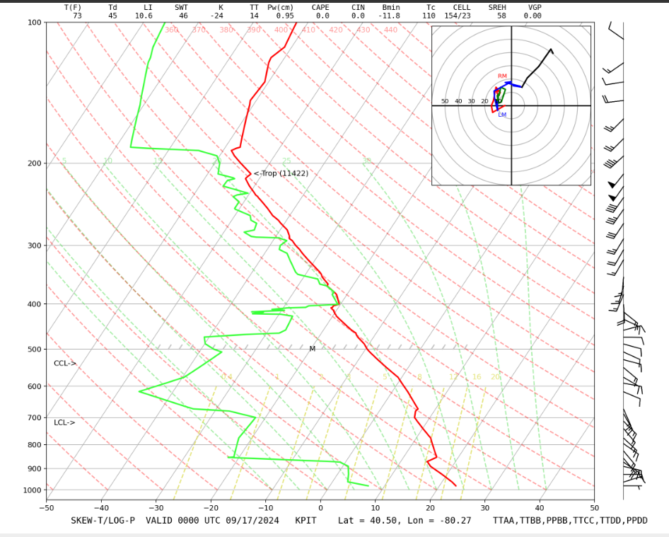
Please also note the following:
- The dry adiabat is the same line as an isentrope (curved red dash lines tilting to the upper left).
- The water vapor mixing ratio is the saturation water vapor mixing ratio at the dewpoint temperature, Td, for each pressure level (gold dot-dash lines tilting to the upper right).
- In clear air, for air parcels moving vertically:
- air parcels move along the dry adiabat and the potential temperature remains constant, even if they contain moisture;
- the water vapor mixing ratio is constant (but notice that Td changes!);
- Td of an air parcel moving vertically (and adiabatically) is decreasing, but not as fast as T of that air parcel is decreasing.
- Eventually, an air parcel moving vertically (along the dry adiabat) will have a temperature and dewpoint temperature that are the same, thus saturated.
- At this altitude level, called the Lifting Condensation Level (LCL), the relative humidity = 100%, T = Td, w = ws, and e = es. At this pressure and temperature, a cloud forms. Actually, the formation of a cloud requires a relative humidity that exceeds 100% by a few tenths of a percent, but we generally use 100% for the skew-T calculations. We will see why this extra relative humidity is necessary in the next lesson.
See the video below (1:19) for further explanation:
Let's see how to find the lifting condensation level, the LCL. The LCL is the level where a cloud will form if the air mass near a surface is pushed upward. We have two quantities that are conserved when lifted. The potential temperature, or theta, and the water vapor mixing ratio, w. As the air parcel is pushed up, then w goes up the constant w line and theta goes up the dry adiabat, which is the constant theta line. Note that both the temperature and the dew point temperature are changing and getting closer to each other as the air parcel ascends. When the two lines meet, the relative humidity is 100%, a cloud forms, and this is the lifting condensation level. Once the LCL has been reached and the cloud is formed, any further ascent will be in the cloud. The air parcel temperature will follow the moist adiabat, which is less than the dry adiabat. Because as water condenses it gives up its energy to warm the air a little bit. If the air were pushed down, its temperature would follow the moist adiabat, as long as it was above the LCL. But below the LCL, it will follow the dry adiabat. And the water vapor mixing ratio will follow the constant w line.
Moist Adiabat
When the air parcel is in a cloud, ascent causes a temperature decrease while the air remains saturated (i.e., w = ws, RH = 100%). Since ws decreases, the amount of water in the vapor phase decreases while the amount in the liquid or solid phase increases, but the total amount of water is constant (unless it rains!). As water vapor condenses, energy is released into the air and warms it a little bit. Thus, the lapse rate of the moist adiabat (curved dot-long-dash green lines tilting toward the upper left) is less than the lapse rate of the dry adiabat (9.8 K/km).
As long as it doesn’t rain or snow, an air parcel will move up and down a moist adiabat as long as it is in a cloud and will move up and down a dry adiabat when w < ws below the LCL.
- Once a cloud forms, any further rise of the air parcel will follow the moist adiabat (condensation of water vapor heats the air so that the temperature decrease with height is less than that of the dry adiabat). As long as the ascent is in the cloud, the relative humidity will remain near 100% and w = ws(T). Since T decreases on ascent, ws decreases, and more water goes into the liquid or ice phase.
- If the air parcel, containing the liquid or ice that was formed, descends, it will move along the moist adiabat until it again reaches the LCL, at which point all of the liquid water or ice will have evaporated or sublimed. Just below the LCL, all of the water will be vapor and the air parcel will descend along the dry adiabat and the water vapor mixing ratio will be constant.
The following is a summary for air parcel ascent and descent:
- From the initial p, T, and Td (or w), locate two points on the skew-T: (1) p and T and (2) p and Td (or w).
- Starting at the first point, move the parcel up the dry adiabat.
- Starting at the second point, move the parcel up the constant-w line. Note that Td is continually changing, so use w.
- Where the two lines intersect is the LCL.
- A cloud will form.
- If the air parcel continues to rise inside the cloud,
- w will always equal ws.
- the air parcel will follow the moist adiabat.
- If the parcel then descends,
- it will follow the moist adiabat down to the LCL.
- it will follow the dry adiabat below that.
- w will follow the w line below that.
The following video (1:43) discusses the process of adiabatic cooling and heating.
We've all seen clouds build up on one side of the mountain and then on the other side just dissipate into blue sky. Maybe you want to know why that happens. Like most natural events, this one has an impressive scientific term attached to it. It's called adiabatic cooling and heating, and occurs because of changes in air pressure. Here's some time lapse video that shows what happens. Basically, as a parcel of air encounters a mountain, it is forced upward. As air pressure decreases with altitude, the air parcel expands. Expansion causes air to cool. When the air cools to its so-called dew point, the water vapor in the air condenses and becomes visible as a cloud. If there's enough moisture and the adiabatic cooling is strong enough, it rains or snows. Essentially the opposite occurs on the other side of the mountain. The cool air sinks and compresses. Compression results in increased temperature. When temperature rises above the dew point, the cloud dissipates into invisible water vapor. In Wyoming, especially in winter, most of the moisture-laden air masses come from the Pacific, approaching our mountains from the west. So as adiabatic cooling occurs, more rain and snow is dumped on west-facing slopes. As warmer, drier air descends on the eastern slopes, it accounts for another famous phenomenon of the plains, the so-called Chinook winds. So we've looked at clouds from both sides now. Knowing why they form and disappear does not diminish their beauty. But if it weren't for our mountains and the dynamic processes that occur, one, we would be a much drier place, and frankly, much less interesting. I'm Tom Hill from the University of Wyoming Cooperative Extension Service exploring the nature of Wyoming.
Other Potential Temperatures
There are other potential temperatures that are useful because they are conserved in certain situations and therefore can help you understand what the atmosphere is doing and what an air parcel is likely to do.
Virtual Potential Temperature
Virtual potential temperature is the potential temperature of virtual temperature, where density differences caused by water vapor are taken into account in the virtual temperature by figuring out the temperature of dry air that would have the same density:
This quantity is useful when comparing the potential temperatures (and thus densities) of air parcels at different pressures.
Wet Bulb Potential Temperature
The wet-bulb temperature is the temperature a volume of air would have if it were cooled adiabatically while maintaining saturation by liquid water; all the latent heat is supplied by the air parcel so that the air parcel temperature, when it descends to 1000 hPa, is less than its temperature would be had it descended down the dry adiabat.
The wet bulb temperature at any given pressure level is found by finding the LCL and then bringing the parcel up or down to the desired pressure level on the moist adiabat.
The wet bulb potential temperature, Θw, is the wet bulb temperature at p = 1000 hPa.
How can we use the wet bulb potential temperature? The wet bulb potential temperature is conserved, meaning it does not change, when an air mass undergoes an adiabatic process, such as adiabatic uplift or descent. If we consider large air masses that acquire similar temperature and humidity, then this entire air mass can take on the same wet bulb potential temperature. Colder, drier air masses will have a lower Θw. The Θw of this air mass can change if a diabatic process occurs, such as the warming of a cold air mass as it moves over warmer land, or the cooling of an air mass by radiating to space during the night, but these processes can sometimes take days. So an 850-mb map of Θw is one indicator of air masses and the fronts between air masses.
See the video below (:32) for further explanation:
Let's see how to find the wet-bulb potential temperature on the Skew-T. The first step is to find the LCL. Once we find the LCL, then we have a saturated air parcel. And it's temperature is the wet-bulb temperature. To find the wet-bulb potential temperature, we simply follow the moist adiabat down to a pressure of 1,000 millibar. We see that the wet-bulb potential temperature is about 19 C, while the potential temperature is about 34 C.
Equivalent Potential Temperature
The equivalent potential temperature is the temperature that an air parcel would have if it were lifted adiabatically until all of the vapor were condensed and removed, and then brought to 1000 hPa adiabatically. For example, let's say you have an air parcel with some water vapor in it below the LCL. To find the equivalent potential temperature, you would (1) lift the parcel to the LCL along a dry adiabat, (2) lift the parcel along the moist adiabat all the way to the stratosphere so that all the water vapor condensed into liquid, and (3) bring the parcel down to 1000 hPa along the dry adiabat. Equivalent potential temperature accounts for the effects of condensation or evaporation on the change in the air parcel temperature.
Every 1 g/kg (g water vapor to kg of dry air) causes Θe to increase about 2.5 K. So, a moist air parcel with w = 10 g kg-1, which is not uncommon, will have Θe that is 25 K greater than Θ.
Approximately,
where Θ is the potential temperature, lv is the latent heat of vaporization, w is the water vapor mixing ratio, and cp is the specific heat capacity at constant pressure.
How can we use the equivalent potential temperature? The equivalent potential temperature, Θe is conserved when an air parcel or air mass undergoes an adiabatic process, just like the wet bulb potential temperature, Θw, is. Note also the total amount of water in vapor, liquid, and ice form is also conserved during adiabatic processes. The total amount of water is quantified using the total water mixing ratio, wt, which is defined in the same way that the water vapor mixing ratio (w) is defined except that it also includes liquid and solid water in the numerator. So, if we look at Θe and wt, we can learn a lot about the history of an air parcel. These conserved quantities are very useful to understand the history of air parcels around clouds. For example, if Θe changes but wt is constant, then the air parcel was either heated or cooled by a non-adiabatic process. On the other hand, if both Θe and wt change proportionally, then two air parcels with different initial values for Θe and wt have mixed. On a larger, more synoptic scale, gradients in Θe can be used to indicate the presence of fronts.
Another use of Θe is as an indicator of unstable air. Air parcels that have higher Θe tend to be unstable. Thus regions of high-Θe air are regions where thunderstorms might form if the surface heating is great enough to erase a temperature inversion.
See the video (1:01) below for further explanation:
Let's see how to find the equivalent potential temperature, called theta-e, on this Skew-T. The equivalent potential temperature is the potential temperature that an air parcel would have if all this water vapor were converted to liquid water, thus warming the air. And then the liquid water was removed. To find theta-e, we find the LCL. Go up to the moist adiabat until it's parallel with the dry adiabat. And then go down the dry adiabat that matches the moist adiabat until we reach the pressure of 1,000 millibar. In this case, theta-e is about 330 Kelvin, or 57 degrees C. Note that the lines aren't marked with such high temperatures. But we can determine which temperature this line represents by looking at the 360 Kelvin dry adiabat. And then counting one, two, three lines over, where the lines are in intervals of 10 K.
Quiz 3-4: Using the skew-T.
- Find Practice Quiz 3-4 in Canvas. You may complete this practice quiz as many times as you want. It is not graded, but it allows you to check your level of preparedness before taking the graded quiz.
- When you feel you are ready, take Quiz 3-4. You will be allowed to take this quiz only once. Good luck!
3.6 Understanding the Atmosphere’s Temperature Profile
3.6 Understanding the Atmosphere’s Temperature Profile
Now we can begin to understand the reasons for the troposphere’s typical temperature profile. The atmosphere is mostly transparent to the incoming solar visible radiation, so Earth’s surface warms, and thus warms and moistens the air above it. This warm, moist air initially rises dry adiabatically, and then moist adiabatically once a cloud forms. Different air masses with different histories and different amounts of water mix and the result is a typical tropospheric temperature profile that has a lapse rate of (5–8) K km-1.
If atmospheric temperature profiles were determined only by atmospheric moisture, drier air masses would have lapse rates that are more like the dry adiabatic lapse rate, in which case we would expect that the skies would have fewer, thinner clouds. Moister air masses would have lapse rates that are closer to the moist adiabatic lapse rate, resulting in a sky filled with clouds at many altitudes.
But many processes affect the temperature of air at different altitudes, including mixing of air parcels, sometimes even from the stratosphere, and rain and evaporation of rain. Exchange of infrared radiation between Earth’s surface, clouds, and IR-absorbing gases (i.e., water vapor and carbon dioxide) also plays a major role in determining the atmosphere’s temperature profile, as we will show in the lesson on atmospheric radiation.The resulting atmospheric profiles can have local lapse rates that can be anywhere from less than the dry adiabatic lapse rate to greater than the moist adiabatic lapse rate. Look carefully at the temperature profile below. You will see evidence of many of these processes combining to make the temperature profile what it is.
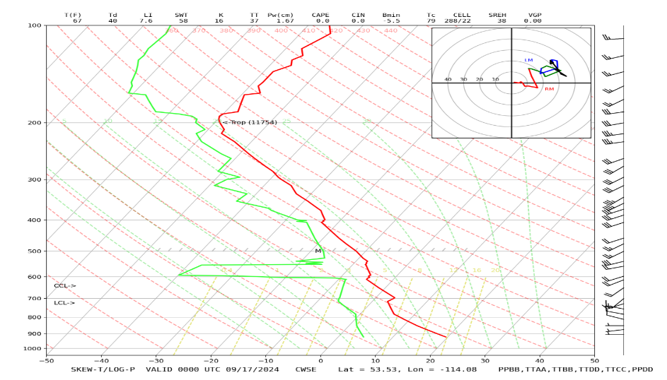
If we average together all of these profiles over the whole year and over the whole globe, we can come up with a typical tropospheric temperature profile. According to the International Civil Aviation Organization (Doc 7488-CD, 1993), the standard atmosphere has a temperature of 15 oC at the surface, a lapse rate of 6.5 oC km–1 from 0 km to 11 km, a zero lapse rate from 11 km to 20 km, and a lapse rate of –1 oC km–1 from 20 km to 32 km in the stratosphere (i.e., temperature increases with height). Even though this standard profile is a good representation of a globally averaged profile, it is unlikely that such a temperature profile was ever seen with a radiosonde.
Combining knowledge of stability along with the knowledge of moist processes enables us to understand the behavior of clouds in the atmosphere. The following picture of water vapor released from a cooling tower at the Three-Mile Island nuclear reactor near Harrisburg, PA shows the water vapor quickly condensing to form a cloud. The cloud ascends, but then reaches a level at which its density matches the density of the surrounding air, the Equilibrium Level (EL). It still has kinetic energy, so keeps rising but increasingly slowly as its density becomes greater and greater than its surroundings. It then descends again, oscillating about the equilibrium level until it eventually settles there. The cloud then begins to spread out.

Summary and Final Tasks
Summary and Final Tasks
Water vapor is a key atmospheric constituent that is essential for weather. There are many ways to express and measure the amount of atmospheric water vapor—specific humidity, water vapor mixing ratio, partial pressure, relative humidity, and dewpoint temperature—and these are all related and can be used interchangeably, although some provide more physical insight than others depending on the question being asked. Water’s most important characteristic in the atmosphere is that it can change phases between vapor, liquid, and ice. In the atmosphere, water is either in the vapor phase or trying to establish an equilibrium between vapor and liquid or vapor and ice. The equilibria conditions are given by the Clausius–Clapeyron equation, which shows that the equilibrium (a.k.a. saturation) water vapor pressure depends only on the temperature. Water phase changes pack a big energy punch and drive weather events. We can calculate the atmospheric temperature changes resulting from phase changes and then see that these temperature changes greatly affect the buoyancy of air parcels and therefore their vertical motion.
A good way to visualize atmospheric vertical structure and behavior is the skew-T diagram. With it, we can readily deduce atmospheric properties and predict what weather is likely to happen if solar heating causes some air near the surface to ascend. Some of the most important properties found using the soundings on the skew-T are the lifting condensation level, the potential temperature, and the equivalent potential temperature. The behavior of a typical sounding on the skew-T shows that the troposphere’s thermal structure is caused in large part by adiabatic ascent and descent, although we will see later that absorption and emission of infrared radiation by water vapor and carbon dioxide also have a hand in shaping the temperature vertical profile.
Reminder - Complete all of the Lesson 3 tasks!
You have reached the end of Lesson 3! Make sure you have completed all of the activities before you begin Lesson 4.
Lesson 4: Atmospheric Composition
Overview
Overview
The atmosphere consists mostly of dry air—mostly molecular nitrogen (78%), molecular oxygen (21%), and Argon (0.9%)—and highly variable amounts of water vapor (from parts per million in air to a few percent). Now we will consider gases and particles in the atmosphere at trace levels. The most abundant of the trace gases in the global atmosphere is carbon dioxide (~400 parts per million, or 400 x 10-6), but there are thousands of trace gases with fractions much less than a few parts per million. Some, particularly the reactive hydroxyl (OH) radical, are important even though their abundance is less than 1 part per trillion (10–12). The atmosphere also contains small particles with sizes from nanometers (10–9 m) to microns (10–6 m) coming from many sources. These trace gases and particles are as important to atmospheric structure and weather as are nitrogen, oxygen, and water vapor and they also play a huge role in human and ecological health and global climate. In this lesson we will examine the atmosphere’s composition and its changes over time. The atmosphere is continually inundated with surface emissions of gases and particles (and some from space) but it has chemical mechanisms to clean itself. We will see how two atmospheric pollutants—ozone and small particles—are produced. In later lessons, we will see that without these chemical processes and particles, there would be no clouds and, thus, no real weather.
Learning Objectives
By the end of this lesson, you should be able to:
- explain the role that each of several atmospheric constituents plays in atmospheric structure and weather
- identify changes in minor and trace gas amounts and the impacts these changes have on the atmosphere
- explain how the atmosphere cleanses itself using methane as an example
- use chemical equations to show how ozone is formed in the stratosphere and the troposphere and how they differ
- diagram the lifecycle of aerosol particles with an emphasis on their role in weather
Questions?
If you have any questions, please post them to the Course Questions discussion forum. I will check that discussion forum daily to respond. While you are there, feel free to post your own responses if you, too, are able to help out a classmate.
4.1 Atmospheric Composition
4.1 Atmospheric Composition
The major gases that comprise today's atmosphere are listed in the table below. In most studies of atmospheric composition, the volume mixing ratio is used to specify the amount of a gas. The volume mixing ratio (also called the molar mixing ratio) of a gas is the number of moles of the gas divided by the number of moles of air. For example, 78 moles of every 100 moles of air is nitrogen, so nitrogen's volume mixing ratio is 0.78.
| Constituent |
Molecular Mass (g mol–1) |
Volume Mixing Ratio (mol mol–1) |
Role in the Atmosphere |
|---|---|---|---|
| nitrogen (N2) | 28.013 | 0.7808 | transparent; provides heat capacity and momentum; exchanged with biomass; decomposed in combustion |
| oxygen (O2) | 31.998 | 0.2095 | transparent except in the extreme ultraviolet; provides some heat capacity and momentum; exchanged with life; source of important reactive gases like ozone |
| argon (Ar) | 39.948 | 0.0093 | no role |
| carbon dioxide (CO2) | 44.010 | 0.000385 (385 ppmv) | transparent in visible; absorbs infrared light (i.e., contributes to global warming); exchanged with life; product of combustion |
| neon (Ne) | 20.183 | 0.0000182 | no role, but makes colorful glowing signs |
| water vapor (H2O) | 18.015 | 2 x 10⁻⁶ to 0.05 | transparent in visible; absorbs infrared light (i.e., contributes to global warming); exchanges with liquid and solid forms; exchanges with life; product of combustion |
| aerosol particles | varies | 0–500 µg m–3 (note different units) | essential for cloud formation; interact with visible and infrared light; exchange with surfaces and life |
| methane (CH4) | 16.04 | 0.00000182 (1820 ppbv) | transparent in visible; absorbs in infrared (i.e., contributes to global warming); exchange with life; source of CO2 and H2O |
| ozone (O3) | 48.00 | 0.01–10 x 10–6 (10 ppbv to 10 ppmv) | transparent in visible; absorbs in UV and infrared; reactive and source of more reactive gases |
| particles | varies | 0–100’s µg m–3 (note different units) | absorb and scatter light; act as CCN and IN (see below) |
Key features of the gases include their compressibility (i.e., ability to expand or shrink in volume), their transparency in the visible, their momentum, and their heat capacity. Key greenhouse gases—those that absorb infrared radiation and hence warm the planet—are water vapor, carbon dioxide, methane, and ozone. Water vapor has the additional important feature of exchanging with liquid and solid phases in the atmosphere and on Earth’s surface. The most important properties of small particles include their ability to dissolve in water in order to be cloud condensation nuclei (CCN) or to maintain a lattice structure similar to ice in order to be ice nuclei (IN), as well as their ability to absorb and scatter sunlight. These properties depend completely on the particle size and composition. Most atmospheric gases participate in the atmosphere's chemistry, which is initiated by sunlight, as you will soon see.
A note on the units used when quantifying atmospheric composition
The amount of a gas is typically specified in one of three different ways. You have already been introduced to the first, the volume mixing ratio, in the table above. For gases with relatively large fractions like nitrogen, oxygen, and argon, we use percent to indicate this fraction. For minor gases like carbon dioxide and ozone, we use parts per million (10–6) by volume (ppmv) or parts per billion (10–9) by volume (ppbv). The second is the mass mixing ratio, which is the mass of a chemical species divided by the total mass of air. You have already encountered this ratio with the specific humidity. The third way to specify the amount of a gas is the concentration, which is the number of molecules per unit volume.
It is straightforward to convert between volume mixing ratio and concentration. For a species X, to convert from a volume mixing ratio, notated χX, to a concentration, notated [X], use the Ideal Gas Law to find the number of total molecules in a cm3 and then multiply by χX, expressed as a fraction. For example, let p = 960 hPa, T = 296 K, and χX = 60 ppbv, then the concentration can be calculated as follows:
Here we have used the Boltzmann constant k, which is simply the universal gas constant divided by Avogadro's number.
4.2 Changes in Atmospheric Composition
4.2 Changes in Atmospheric Composition
Since the Earth was formed more than 4 billion years ago, the atmosphere has changed profoundly. A wide variety of geochemical and ecological (fossil) evidence indicates that oxygen levels rose dramatically about 2 billion years ago. Such evidence also indicates that carbon dioxide levels were much higher earlier in Earth's history, which allowed the Earth to be at a habitable temperature despite the fact that the output from the Sun was much lower (about 25%) compared to today, resolving the so-called "Faint-Young-Sun Paradox." Below we discuss changes in atmospheric composition over the past 800,000 years, the past few hundred years, and the past several decades.
Changes over the past 800,000 years
We have learned a lot about how atmospheric composition has changed from measurements of gases in bubbles trapped in ice cores. The figure below, which shows such measurements from an Antarctic ice core, reveals that two key greenhouse gases, CO2 and CH4, underwent large, rapid variations over the past 400,000 years. The variations are also periodic, with a rapid decline followed by a more gradual increase every 100,000 years or so, and are in roughly in phase with the temperature and out of phase with ice volume. The periodic variations reflect the coming and going of the ice ages. Similar cycles have been measured as far back as 800,000 years for CO2 and CH4 and other fossil evidence suggests that the current period of ice ages that we are in now began about 2.6 million years ago. These changes in CO2 and CH4 were driven ultimately by changes in the Earth's orbit and axis of rotation, which led to changes in the amount of solar radiation received at various latitudes during various seasons. Summer solar radiation at high northern latitudes is particularly important (bottom curve below), because it regulates how the large northern hemisphere ice sheets grow. These changes in solar radiation led to changes in Earth's temperature, ocean circulation, and other processes that influence atmospheric CO2 and CH4, which amplified the changes in Earth's temperature.
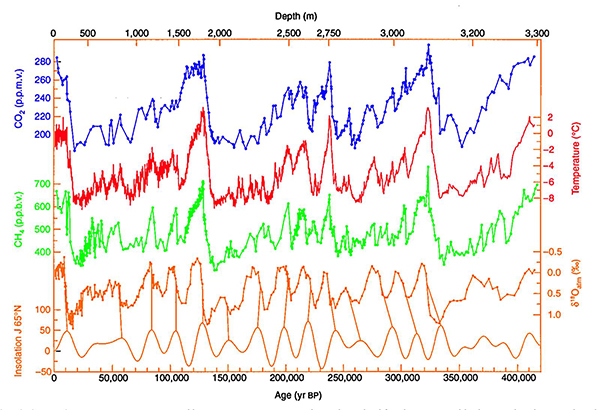
Changes over the past few hundred years
The Holocene period began about 12,000 years ago, at the end of the last ice age, and marks a period of relative stability in climate and atmospheric gas concentrations. During this time, the ice core data reveal that levels of CO2 and CH4 in the atmosphere were relatively constant, at about 280 ppmv and 650 ppbv, respectively. Then, as shown below, levels of both gases, as well as another greenhouse gas, nitrous oxide (N2O), increased rapidly about 200 years ago. These increases, which coincide with the industrial revolution, were due to anthropogenic activity, including the burning of fossil fuels and enhanced deforestation and agriculture. The increases in these three greenhouse gases are the primary cause of the warming of the Earth by about 1 oC over the past century.

Ice core data reveal many other interesting changes in the atmosphere that occurred during the last 200 years or so, particularly in the Northern Hemisphere. For example, within the ice itself, one can see increases in the amount of nitrate and sulfate [38], which are produced ultimately from the combustion of fossil fuels. These constituents are the key components of acid rain and, indeed, data from the same ice core also reveal an increase in acidity.
Changes over the past several decades
Changes in the composition of the atmosphere over the past several decades primarily reflect changes in human activity.
As fossil fuel emissions have increased over recent decades, so has the growth rate of atmospheric CO2, as indicated by the concave-upward curvature in the figure below. The growth rate has approximately doubled from about 1 ppmv per year in the 1960s to about 2 ppmv per year in the 2000s. According to the Global Carbon Project [39], 86% of the anthropogenic CO2 emissions during 2009–2018 were from fossil fuel burning and 14% were from land-use change (e.g., deforestation). However, CO2 injected to the atmosphere from human activity does not stay there. 44% of the emissions from human activity during 2009–2018 accumulated in the atmosphere, 29% were absorbed by terrestrial ecosystems, 23% were absorbed by the ocean, and 4% is unaccounted for (Global Carbon Project). Superimposed on the accelerating trend over the past few decades is an annual cycle in which CO2 declines during Northern Hemisphere summer and rises during most of the rest of the year. This cycle reflects photosynthesis (an atmospheric CO2 sink) and respiration (an atmospheric CO2 source) of terrestrial ecosystems in the Northern Hemisphere, where most land is present. Note that the current increase to above 400 ppmv now extends well above any other time in the past half 800,000 years, at least, when CO2 varied between about 180 and 280 ppmv.

The changes in methane over the past several decades are more complex than those of carbon dioxide. The figure below shows that the methane growth rate (the slope of the curve) gradually declined from the 1980s to roughly zero by the mid 2000s. Since then, the growth rate has increased, though it is still not as high as it was in the 1980s. A detailed budget of methane has been developed by the Global Carbon Project [39] and indicates that for 2008–2017 about 60% of the methane sources were anthropogenic (mainly from agriculture, waste, fossil fuel production and use, and biomass burning) and 40% were natural (mainly from wetlands, inland waters, geological sources, ocean, termites, wild animals, permafrost, and vegetation). The main sink of methane is oxidation by OH, which we will discuss later in this lesson, as well as consumption within soils. Despite our basic understanding of methane sources and sinks, we do not know why the methane growth rate has changed in the way it has over the past several decades. This is an important unresolved problem, because methane levels are very high currently. In 2019, the global-average methane mixing ratio was more than 1860 ppbv, which is well above values over the last 800,000 years, at least, which varied between about 400 and 700 ppbv.

Numerous lines of evidence show that water vapor is increasing in the atmosphere. Surface specific humidity measurements, which have been made mostly in the Northern Hemisphere, show clear trends, as indicated in the figure below. Data from satellites indicate that precipitable water (the total amount of water that is in a column from the surface to the top of the atmosphere) increased 1.49% per decade from 1988 to 2017 (Mears et al., 2005) [41]. These trends are generally consistent with expectations of a warming world and the Clausius–Clapeyron equation. Variability from year to year is also consistent with temperature change. For example, the increases in temperature resulting from the very large 1997–1998 El Niño event were accompanied by large increases in surface specific humidity and total precipitable water.

There are trends and variations in many of the other trace gases as well, such as chlorofluorcarbons, which are decreasing in abundance due to emissions reductions. There are other trace gases that increase as the sun rises and decrease as it sets and are heavily involved in atmospheric chemistry. We will talk about these gases next.
4.3 Other Trace Gases
4.3 Other Trace Gases
Hundreds of different trace gases have been measured in the atmosphere and perhaps thousands more have yet to be measured. Many of these are volatile organic compounds (VOCs). Volatile means that the compound may exist in the liquid or solid phase but that it easily evaporates. Organic means that the compound contains carbon but is not carbon dioxide, carbon monoxide, or carbides and carbonates found in rocks. There are also other chemicals like the nitrogen oxides (e.g., nitric oxide (NO), nitrogen dioxide (NO2), nitric acid (HNO3)), sulfur compounds (e.g., sulfur dioxide (SO2), sulfuric acid (H2SO4)) and halogen compounds (e.g., natural methyl chloride (CH3Cl), human-made chlorofluorocarbons (CCl2F2)). If we pay attention, we can often smell and identify many of these chemicals, even at trace levels, although some, like methane, carbon monoxide (CO), and chlorofluorocarbons, are odorless. We enjoy smelling the VOCs emitted by trees in a forest—aah, that fresh pine smell—but we hold our nose to escape the smells of a stagnant swamp.
In addition to these thousands of chemicals that are emitted into the atmosphere every day, there are also some very reactive compounds that are created by atmospheric chemistry and play the important role of cleaning the atmosphere of many gases. The most important reactive gases are ozone (O3) and hydroxyl (OH). We will focus the discussion of atmospheric chemistry on these two.
The Atmosphere’s Oxidizing Capacity
Earth’s atmosphere is an oxidizing environment. This term means what you think it would: gases that are emitted into the atmosphere react in a way that increases their oxygen content. Gases that contain oxygen tend to be “stickier” on surfaces and more water soluble, which means that they stick when they hit a surface or they can be readily taken up in clouds and rain drops and be deposited on Earth’s surface. We call gases hitting the surface and sticking “dry deposition” and gases being taken up in precipitation and rained out “wet deposition.”
Let’s consider a natural gas that is very important in our lives, methane, also known as natural gas. More and more methane is being extracted from below Earth’s surface and used to run our electrical power plants, heat our homes, cook our food, and, increasingly, to run our transportation vehicles. Methane is a simple molecule, CH4, in which each of carbon’s four bonds is made with a hydrogen atom. Energy comes from heating methane to high enough temperatures that cause it to react, giving off energy as more stable molecules are formed. In complete combustion, each methane molecule is converted into one CO2 molecule and two H2O molecules. In the process, four oxygen atoms or two oxygen molecules are consumed.
This same process occurs in the atmosphere, but at much lower temperatures and at a much slower rate. In both cases, the first step in the methane oxidation sequence is the reaction with the hydroxyl radical (OH). In water, hydroxyl loses an electron and is ionized (OH–), but in the atmosphere, hydroxyl is not ionized. We call OH a free radical because it has an odd number of electrons (eight for oxygen and one for hydrogen). Any gas with an odd number of electrons is reactive because the electrons want to be paired up in molecules because that makes them more stable.
Often, combustion is inefficient, resulting in the formation of carbon monoxide (CO). Examples include forest fires, humans burning fields to clear them for planting, poorly tuned vehicles, inefficient industrial processes, and other human-caused processes. The primary way that CO is removed from the atmosphere is by reacting with atmospheric OH. It takes a while for CO to be removed from the atmosphere by the reaction with OH, so that satellite instruments can track CO plumes as they emerge from their sources and flow around the world.
Where does OH come from?
Before we tackle this question, let’s first look at where ozone (O3) comes from. We will start with stratospheric ozone (a.k.a. good ozone because it blocks solar UV that harms humans, other animals, agriculture, and ecosystems) and then eventually we will consider tropospheric ozone (a.k.a. bad ozone, which is the ozone that hurts our health when we breathe it and that damages plants and their fruit).
Discussion Forum 2: Trace gases
For this week's discussion activity, I would like you to think about which trace gas is the most important and why. By trace gas I mean a gas with a mixing ratio of less than 20 ppm in the atmosphere. Defend your choice. Use information from this lesson as well as other sources (credit them, please!) to describe the qualities of this gas that make you think that it is the most important trace gas. Then read the choices of your classmates and respond to their choices and follow-up with further questions and/or analysis.
- You can access the Trace gases Discussion Forum in Canvas.
- Post a response that answers the question above in a thoughtful manner that draws upon course material and outside sources.
- Keep the conversation going! Comment on at least one other person's post. Your comment should include follow-up questions and/or analysis.
This discussion will be worth 3 discussion points. I will use the following rubric to grade your participation:
| Evaluation | Explanation | Available Points |
|---|---|---|
| Not Completed | Student did not complete the assignment by the due date. | 0 |
| Student completed the activity with adequate thoroughness. | Student answers the discussion question in a thoughtful manner, including some integration of course material. | 1 |
| Student completed the activity with additional attention to defending their position. | Student thoroughly answers the discussion question and backs up reasoning with references to course content as well as outside sources. | 2 |
| Student completed a well-defended presentation of their position, and provided thoughtful analysis of at least one other student’s post. | In addition to a well-crafted and defended post, the student has also engaged in thoughtful analysis/commentary on at least one other student’s post as well. | 3 |
4.4 Stratospheric Ozone Formation
4.4 Stratospheric Ozone Formation
Ozone is ozone no matter where it is in the atmosphere. Good ozone is good only because it is in the stratosphere where we cannot breathe it (see figure below). Bad ozone also absorbs solar ultraviolet light, but it is down near Earth's surface where we can breathe it. For UV protection, we are interested in the total number of ozone molecules between us and the Sun. 90% of ozone molecules are in the stratosphere and 10% are in the troposphere—some down near Earth's surface where we can breathe them. There are important issues affecting human and ecological health for both good ozone and bad ozone. For good ozone, the most important issues are the reduction of ozone globally, the Antarctic Ozone Hole, and Arctic ozone loss that is caused by chlorofluorocarbons. Reduced ozone means more solar UV gets to the ground causing more skin cancer. For bad ozone, the most important issues include the production of too much ozone in cities and nearby regions that is caused by too many pollutants from traffic, industrial processes, power generation, and other human activities. Increased ozone means more people have respiratory and heart problems. Let's look at both the good and the bad, starting with the stratospheric ozone.

Explanation diagram of the typical vertical ozone profile for the tropics
Stratospheric Ozone (the ozone layer, ~15–35 km)
- contains 90% of atmospheric ozone
- beneficial role: acts as primary UV radiation shield
- Current issues
- long-term global downward trends
- springtime Antarctic ozone hole each year
- springtime arctic ozone losses in several recent years
Tropospheric Ozone (0–15 km)
- contains 10% of atmospheric ozone
- harmful impact: toxic effects on humans and vegetation
- current issues
- episodes of high surface ozone in urban and rural areas
To get the total amount of ozone between us and the Sun, we simply add up the ozone amount starting at the surface and going up to the top of the ozone layer. Note how much more ozone there is in the stratosphere. At higher latitudes, the bottom of the stratospheric ozone layer is at approximately 10–12 km. Recall the following image from Lesson 2:
The process of stratospheric ozone formation starts with ozone (O3), which is made by ultraviolet sunlight in the stratosphere (but not the troposphere, as we shall see). The two reactions are:
Note that N2 doesn't really react in this last chemical equation, but instead, simply bumps into the O3 molecule as it is being formed and stabilizes it by removing some of the energy from O3. We call O3 an oxidant because it can react with some compounds and oxidize them.
This O3 can be broken apart by ultraviolet light to make O2 and O. Usually O combines with O2 to form O3 in this way: O + O2 + N2 → O3 + N2, so nothing really happens, except that the solar energy that breaks apart the O2 ends up as extra energy for the O3 and for the colliding N2 and, as a result, ends up warming the air. Sometimes O collides with O3 and reacts as follows: O + O3 → O2 + O2. Putting all of the reactions together, we can see the chemical lifecycle of ozone in the stratosphere. This set of reactions was proposed in the 1930s by Chapman:
| O2 + UV → O + O | production |
| 2(O + O2 + N2 → O3 + N2) | cycling |
| O3 + UV → O2 + O | |
| O + O3 → O2 + O2 | loss |
| Net: UV → higher T | |
These four reactions could produce the basic characteristics of the ozone layer as it was in the 1940s through the 1970s. The basic ingredients are UV radiation and O2, which can help to explain why ozone reaches a maximum concentration at a certain height in the atmosphere–that is, why there is an ozone layer at all. At very high levels in the atmosphere (e.g., in the mesosphere), there is plenty of UV but too little O2 (simply because pressure decreases with height). On the other hand, at very low levels in the atmosphere (the troposphere), there is plenty of O2 but very little UV (because of absorption by O2 above). It's only in the stratosphere that there is enough of both UV and O2 to make plenty of ozone.
While Chapman's theory predicted the existence of an ozone layer, the theory produced peak ozone levels that were 50 milliPascals (mPa), not the 25–30 mPa seen in the first figure above. Thus, the measured levels of stratospheric ozone were about half of those predicted by Chapman's theory—it was a real puzzle. However, in the 1970s, scientists proposed new sets of reactions by other gases that accomplished the same results as the loss reaction shown above. A famous example involved chlorine, which comes mostly from human-made chlorofluorocarbons (CFCs):
| CFCs + UV → product + Cl | production |
| Cl + O3 → ClO + O2 | cycling |
| ClO + O → Cl + O2 | |
| Cl + CH4 → HCl + CH3 | loss |
| Net: O3 + O → O2 + O2 | |
During the cycle, chlorine (Cl) and chlorine monoxide (ClO) aren’t destroyed but instead are just recycled into each other. With each cycle, two ozone molecules are lost (one directly and a second because O almost always reacts with O2 to form O3). This cycle can run for hundreds of thousands of times before Cl gets tied up in HCl. So ClO and Cl levels of tens of parts per trillion of air (10–12) are able to destroy several percent of the few parts per million of O3. Sherry Rowland and Mario Molina figured this cycle out and wrote a paper about it in 1974. They received a Nobel Prize in Chemistry in 1995 for this work. When catalytic cycles involving chlorine, nitrogen oxides, and OH are included with the theory, the agreement between the theory and the measurements gets much better.

Check Your Understanding
Note that the total ozone amount at midlatitudes is greater than the amount in the tropics. This should seem strange to you because the solar UV that is part of the Chapman mechanism is strongest in the tropics. Why do you think that total ozone is distributed this way?
ANSWER: In addition to the production and destruction processes described above, the ozone distribution in the stratosphere is due to the motion of air. Air comes from the troposphere into the stratosphere mostly in the tropics and then slowly moves to middle and high latitudes, where it sinks and re-enters the troposphere. This air motion is known as the Brewer–Dobson circulation. Even though most ozone is made in the tropical stratosphere, the production process is relatively slow, and hence ozone abundance in the tropical stratosphere is quite low. As the air moves poleward, the production process adds ozone to the air, leading to relatively high ozone abundance at midlatitudes.
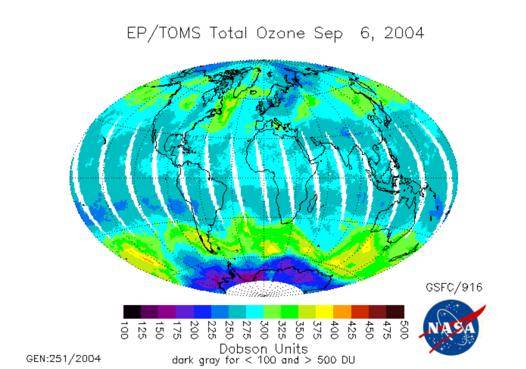
The low ozone over Antarctica above is the Antarctic Ozone Hole; the video below (:31) entitled "Ozone Minimums With Graph" (from NASA) shows changes in ozone concentration between 1979 and 2013. Video is not narrated:
The Antarctic ozone hole is an extreme example of the destructive power of chlorine catalytic cycles. Different catalytic cycles dominate the ozone destruction over Antarctica and, to a lesser extent, the Arctic. But, when aided by chemistry on the surfaces of naturally occurring polar stratospheric clouds, all the Cl in the form of HCl is liberated so that the polar catalytic cycles are able to destroy a few percent of the ozone per day in a plug the size of Antarctica from an altitude of 12 km all the way up to 20 km.
Fortunately, the amount of chlorine being injected into the stratosphere is decreasing due to the Montreal Protocol, the world’s first international global environmental treaty.
4.5 The Story of the Atmosphere's PAC-MAN
4.5 The Story of the Atmosphere's PAC-MAN

The atmosphere's oxidation capacity is its ability to clean itself of all of the gases that are emitted into it. What does stratospheric ozone have to do with the atmosphere’s oxidation capacity, which mostly occurs in the troposphere and mostly by the atmosphere's PAC-MAN, hydroxyl (OH)? It turns out that natural dynamic processes actually pull air down from the stratosphere and mix it into the troposphere, eventually mixing some of this ozone to Earth’s surface. This naturally occurring surface ozone provides a baseline value for near-surface ozone, but ozone pollution is more than ten times greater than this baseline in cities. Ozone is both sticky on surfaces and fairly reactive in the atmosphere. It is lost both by depositing on surfaces and through being chemically destroyed by reactions in the atmosphere.
The following chemical sequences are the humble beginnings of the atmosphere's PAC-MAN. OH is generated throughout the stratosphere and troposphere by a two-step reaction sequence. The first step is:
where O* is an excited-state oxygen atom that has extra chemical energy. O* can lose this extra energy by colliding with N2 and O2, but it can also collide with a water molecule to make two OH molecules:
OH is very reactive. You can think of OH as being water that has had a hydrogen taken away and wants it back. There are other sources for OH, but this one is the most important globally. OH reacts with many other atmospheric constituents. In fact, it is so reactive, that its lifetime in the atmosphere is less than a second.
Another important oxidant is nitric oxide (NO). It comes from combustion (power plants, internal combustion engines, fires) or lightning. In cities, the NO mixing ratio is tens of ppbv during morning rush hour and a bit smaller during evening rush hour, but there is typically about a ppbv around during the day. In very remote areas, the levels of NO are a hundred times less. NO can react with many chemicals, but a particularly important reaction is with O3:
which forms nitrogen dioxide, NO2. NO2 is not very stable:
but the O reacts immediately with O2 to form ozone:
If an NO2 molecule is produced, then an O3 molecule will be produced during the day when the sun is out. Note that if we think of these three reactions as a cycle, no ozone was either created or destroyed because it is destroyed in [4.5] and created in [4.2].
What happens to all of the methane emitted into the atmosphere?
Methane is a volatile organic compound (VOC). Methane oxidation is a good model for what happens to all of the volatile organic compounds that you smell every day and all the ones that you can’t smell. I am not going to show you the entire reaction sequence. Instead, here are just a few steps.
The first step is the reaction between methane and hydroxyl:
Note that water vapor is made and CH3 is a radical because it has 6 + 3 = 9 protons and, therefore, 9 electrons. Just as for most other VOCs and some other trace emissions, the reaction with OH is the main way methane is removed from the atmosphere. Otherwise, it would build up to high abundance.
CH3 is very reactive. It combines with O2:
If there is any NO around, the following reaction happens:
followed by:
and:
The chemical CH2O is formaldehyde. Some of you may have encountered it in high school chemistry or biology and so may be familiar with the smell. You also see that we got the OH molecule back.
Ultimately, formaldehyde gets broken down to CO and the net reaction of methane oxidation is:
Remember that NO2 is easily broken apart by the UV sunlight that reaches Earth’s surface, so we can take this reaction sequence a step further and show that in the presence of sunlight, reactions [4.6] and [4.2] give:
or
In this final chemical equation, we do not see OH, HO2, NO, or NO2, yet they are essential to the formation of ozone. They are catalytic, which means that they are neither created nor destroyed in the reaction sequence, but instead are simply recycled between OH and HO2 and between NO and NO2. There are other reactions that destroy these reactive chemicals by producing other chemicals that are much less reactive and sticky, a main one being:
where HNO3 is nitric acid, a very sticky and water-soluble chemical. However, each OH that is produced can typically oxidize more than ten methane molecules before it reacts with NO2 to form nitric acid. And as reaction [4.13] shows, each time methane is completely oxidized, two O3 molecules are produced. That's a lot of chemical steps to remember, but I don't want you to necessarily remember them. I want you to see that the process started with a reaction of OH with a volatile organic compound (in this case methane) and that in the subsequent reactions, the product molecules had more and more oxygens attached to them. This process is why we say that the atmosphere is an oxidizing environment.
Where does ozone pollution come from?
Ozone is a different sort of pollutant from others because it is not directly emitted by a factory or power plant or vehicle but instead is produced by atmospheric chemistry.
Three ingredients are needed to make ozone pollution: volatile organic compounds (VOCs) (like methane); nitric oxide (NO from combustion); and sunlight. When we say this, we assume that we already have some ozone and water to provide the OH to get the reactions started. Every VOC goes through an oxidation process that is similar to the methane oxidation reaction sequence. In the methane oxidation sequence, steps [4.9] and [4.11] make NO2, which in the presence of sunlight makes ozone through step [4.6] followed by step [4.2]. Voila! Ozone is formed from methane oxidation in the presence of nitrogen oxides and sunlight. Now imagine the thousands of volatile organic compounds in the atmosphere and realize that all of them—both anthropogenic and natural—can participate in the production of ozone pollution. Now you have seen the sequence of chemical reactions that produce tropospheric ozone.
Let's look at a video (3:14) entitled "Ground Level Ozone: What Is It?" that explains ozone production without getting into the gory details of the chemistry.
We're all pretty familiar with what O2 is. I hope so. You need to breathe it to live. Yes, O2 is oxygen, that life-giving gas, but what is O3? O3 is another gas essential to our survival but it's definitely not for breathing. O3 is ozone high up in the stratosphere. It's made naturally and absorbs harmful ultraviolet rays from the Sun. Without it life as we know it wouldn't, couldn't exist. We need the ozone layer in the stratosphere. We want it, we rely on it. But don't get too used to singing ozone's praises. High ozone levels at lower altitudes, what we call the troposphere, where we live and breathe or anything but natural and beneficial. In fact, down here it turns out to be a toxic atmospheric pollutants. Yep, you heard me right. ground-level ozone primarily exists due to human activities that burn fossil fuels. Transportation, our power and industrial plants, and other activities expel nitrogen oxides and hydrocarbons. When those compounds interact with sunlight, voila, ozone is created a contributor to smog. that's why I ozone levels increase during the summer months when sunlight is abundant. Yes, smog love summer just like many of us. We run, bike, hike, fish, play, stroll, oh yeah, and breathe. Yes, the fact that more people are outside when it's warmer makes us particularly vulnerable to Ozone's harmful impacts. Ozone is a harmful oxidant when we inhale it it's like getting a sunburn inside your lungs and it can be particularly serious for the young, old, active, and those with respiratory conditions at any age. And it's not just humans that are vulnerable ozone harms plants, crops, and agricultural yield interfering with pretty important processes like well, photosynthesis and even our economy. To make matters worse ozone production increases with higher temperatures which are occurring more frequently with climate change. The EPA sets national ambient air quality standards for several pollutants in the United States including ground level ozone. When a county is out of compliance they need to know what can be done to improve air quality. and let's not forget that air pollution is a global comments. air pollution is shared from surrounding cities states and also country's halfway around the world. What can we do, what are we willing to do to improve current levels? Drive less, carpool, avoid car idling, set your home's thermostat higher in the summer and lower in the winter, avoid gas powered lawn & garden tools on severe ozone days. There's a lot to do and lots to know about air quality knowing more about the sources and contributors to ozone and other atmospheric pollutants will help us chart our course.
Ozone pollution is bad for the health of people, crops, and forests. Ozone can react with some types of VOCs, including types that make up our lungs, and breathing it can cause serious health problems and even death. Ozone reacts with the VOCs that make up plants and stunts their growth and damages their fruit. The Clean Air Act from the 1970s has dramatically decreased the levels of air pollution in the United States, including ozone. The EPA can take the credit for much of the progress against air pollution in the United States. But there is still a ways to go and the progress may be reversed due to effects of climate change. Since ozone pollution increases at higher temperatures, the increases in global temperatures could actually reverse the steady progress in ozone reduction and ozone pollution could once again increase, unless volatile organic compounds and nitrogen oxides are reduced even more.
Now you can see why OH is called the PAC-MAN of the atmosphere. But how can we tell how long it will take for OH to remove from the atmosphere some trace gas like methane? Let’s look at an equation for the budget of methane. It is produced in the atmosphere by all the emissions from cows and wetlands. It is removed from the atmosphere by reactions with OH [4.7]. The rate of removal, that is the change in the methane concentration with time, is always proportional to the amount of the two reactants, in this case, CH4 and OH. So, the change in methane with time is given by the balance between methane production and methane loss by reaction with OH:
where kOH+CH4 is the reaction rate coefficient (units: cm3 molecule–1 s–1) and [OH] and [CH4] are the concentrations of OH and CH4 (units: molecules cm–3). Note that the production is positive and increases CH4 with time while the loss is negative and decreases CH4 with time.
We use [OH] to indicate the concentration of OH (molecules cm–3), which is quite different from the OH mixing ratio, which is usually expressed in ppt (10–12). Note that 1 ppt ~ 2.4 x 10⁷ molecules cm–3 for typical surface conditions. See the video below (1:47) entitled "Rate Equation" for further explanation:
Let me explain equation 4.15, which is a rate equation for methane. A rate equation is just a differential equation. The change of something with respect to time equals the production rate of something, minus the fraction of something that is lost each unit of time, multiplied by the amount of something. Note that the loss rate of something is always proportional to something. That something can be anything. It does not have to be a chemical concentration. It could be the amount of milk in your refrigerator, or the number of socks in your drawer, both of which tend to disappear over time. And equation 4.15 is the methane concentration, which has units of molecules per centimeter cubed. The production rate is in units of molecules per centimeter cubed per second. Remember, each term of the equation must have the same units. The last term is the loss rate. The reaction rate coefficient has units of centimeter cubed per molecule per second, but when we multiply it by the OH concentration, we get a product that has units of per second, which is a frequency. Now, OH varies from almost 0 at night, to a peak value at midday. However, we can take an average OH to find the average loss rate of methane. Note that if we assume that the production rate suddenly goes to 0, then we find a very simple equation, which has an exponential solution. We designate the time that it takes the exponential factor to go to minus 1 as a lifetime, which is just the inverse of a loss frequency.
How can we find out what the lifetime of methane is? We assume that the production suddenly stops and equals 0. Then [4.15] becomes:
kOH+CH4 is the reaction rate coefficient for this reaction. Assume that OH is constant. Because OH is generated mostly from sunlight, it follows the sunshine and is greatest near midday and is very small at night. However, we assume that the OH concentration is the average over the day and night in order to assign it a constant value. Now integrate both sides of the equation:
So we see that methane decreases exponentially with time.
The lifetime of an atmospheric constituent is defined as the time it takes that constituent to decrease to e–1 = 0.37 of its initial value once production stops. So the lifetime of methane in the atmosphere is the value of t when kOH+CH4[OH]t = 1, or:
where τ indicates the lifetime. kOH+CH4 = 3 x 10–15 cm3 molecule–1 s–1 and [OH] ~ 106 molecules cm–3, so:
This reaction rate coefficient is fairly low. Other VOCs have reaction rate coefficients that are typically hundreds to hundreds of thousands of times greater, so the lifetime of most VOCs is hours to days.
The atmospheric lifetime of a gas is very important for determining how far a gas can travel from its source. Some trace gases have lifetimes of hours, so unless they are made by atmospheric chemistry, they can't travel more than a few tens of kilometers from their sources. Other gases have much longer lifetimes; methane is a good example with its 10-year lifetime. In 10 years, it can travel from its sources to most anywhere around the globe, even to the stratosphere. NASA measures the amounts of several gases from space. An excellent NASA website for accessing these satellite data and having it plotted as global maps is the Center for Trace Gas Data & Information Website at the NASA Goddard Space Flight Center's Earth Sciences Distributed Active Archive Center (GES DISC) [42].
This concept of atmospheric lifetime is very important. For instance, what if an industry is spewing a chemical into the atmosphere that is toxic at a certain concentration in the atmosphere? Then it is important to know if that chemical is removed in less time than it takes to become toxic or if it is going to continue to build up at toxic levels and not leave the atmosphere for a long, long time. If the chemical's atmospheric lifetime is hundreds to thousands of years, then maybe we shouldn’t let that industry dump that chemical into the air.
Now it is your turn to solve some problems concerning the atmospheric lifetimes and rates of change for atmospheric constituents in a quiz.
Quiz 4-1: Atmospheric lifetimes calculations.
- Find Practice Quiz 4-1 in Canvas. You may complete this practice quiz as many times as you want. It is not graded, but it allows you to check your level of preparedness before taking the graded quiz.
- When you feel you are ready, take Quiz 4-1. You will be allowed to take this quiz only once. Good luck!
4.6 Where do cloud condensation nuclei (CCN) come from?
4.6 Where do cloud condensation nuclei (CCN) come from?
Now that you've learned about the atmosphere’s gas-phase composition, it is time to look at its particle composition. We are interested in atmospheric particles for several reasons:
- smaller ones can get into the lungs and cause serious health problems;
- smaller ones can absorb or scatter sunlight, thus affecting climate;
- some of them are good cloud condensation nuclei, which are essential for the formation of clouds.
Atmospheric aerosol is most obvious to us on warm and muggy summer days. Under these conditions, there are lots of aerosol particles and they absorb water and swell up to a size that is quite efficient at scattering sunlight. The following picture was taken over Maryland on a flight between Washington Dulles airport and State College airport. Above the fair-weather cumulus clouds is blue sky in the free troposphere. Below the clouds is the atmospheric boundary layer, which is filled with aerosol that has been well-mixed by warm, moist air parcels rising and stirring the boundary layer air. The haze is so thick that it is a little hard to see the ground.

Atmospheric particles come from many different sources. Good cloud condensation nuclei (CCN) must be small particles, so that they do not settle too fast, and must be hydrophilic, which means that water can stick. They can be either soluble (i.e., dissolvable in water), or insoluble, but most are soluble.
Most particles originate from emissions from Earth’s surface. Primary aerosols are emitted directly from the source, although the smaller ones start off as hot gases that rapidly condense to form particles even before they leave the smokestack or tailpipe. Secondary aerosols are gaseous emissions that are converted to aerosol particles by chemical reactions in the atmosphere. Some of these become CCN. This process is often called gas-to-particle conversion. Most CCN are secondary aerosols.
The sources of aerosols are both natural and anthropogenic (human-made). Seaspray, volcanoes, forests, and forest fires, as well as gas-to-particle conversion of naturally occurring gases such as sulfur dioxide (SO2) and some naturally occurring VOCs, such as α-pinene (which gives the pine smell) are important natural particle sources. Industry, power plants, using fires to clear cropland, transportation, and gas-to-particle conversion of anthropogenic SO2 and numerous other gas emissions are important anthropogenic particle sources.
Note that we must pay attention not only to the aerosol sources but also the aerosol sinks, as shown in the diagram below.

The different sources make particles of different sizes. The typical size distribution (i.e., number of particles in a volume of air, plotted as a function of size) has bumps in it, with more particles at some sizes than at others, as seen in the diagram below. Reading these bumps tells us a lot about how the particles were made.
The nucleation mode (there are other designations for this) includes particles that are made by gas-to-particle conversion. A low-volatility vapor is one that will condense onto particles or other surfaces when its vapor pressure exceeds its low saturation vapor pressure. This situation is analogous to water.
The coarse mode includes particles made by mechanical processes. The hydrophilic coarse particles can be CCN, but they settle out pretty fast.
The accumulation mode includes particles that are usually made when nucleation particles collide and stick (called coagulation) or when gases accumulate on a nucleation mode particle. The accumulation mode particles neither settle fast nor coagulate, so they tend to hang around in the atmosphere for a few weeks. They make pretty good CCN.

PM2.5 - Secondary Particles from Gas-to-Particle Formation
PM2.5 is a particle size designation that means “Particle matter smaller than 2.5 µm in diameter.” Another common term is PM10, which is "particle matter smaller than 10 µm in diameter." PM2.5 particles are the ones that are most important for human health and climate, and, in many cases, cloud formation, because of their longer lifetime in the atmosphere.
Secondary particles start with the emission of VOCs or sulfur compounds, which react mainly with OH to start a sequence of reactions. These reactions tend to add oxygen to the molecules, which chemically makes them stickier (with a lower saturation vapor pressure) and more water soluble, which is just what is needed to make them better cloud condensation nuclei.
For particles that start as gaseous sulfur compounds, such as sulfur dioxide (SO2), the reaction sequence starts with OH and the reaction product is sulfuric acid, a compound that has a very low vapor pressure and is very sticky:
Sulfuric acid is easily taken up into cloud drops and raindrops and then can be deposited on Earth’s surface when it rains. The good news is that the rain cleans the atmosphere. The bad news is that the rain is very acidic and has earned the name “acid rain” because of its harmful effects on forests and on buildings, memorials, and statues.
If sulfur sources are upwind of an area, the particles in that area will contain some sulfur. But almost all atmospheric particles also contain some organic compounds and sometimes particles are mainly made up of carbon-containing organic compounds. Some of these organic particles are primary, but most of the small ones are made by gas-to-particle conversion, which is just a simple way to say the volatile organic compounds react in the atmosphere with OH or O3 to form less volatile organic compounds that become aerosol particles. The chemicals in these particles can continue to oxidize, thus making them even better CCN.
We can demonstrate gas-to-particle conversion of a VOC that is often emitted into the atmosphere by trees. This compound is limonene and also comes from oranges. In the video (4:47) below entitled "Demonstration of Gas-to-Particle Conversion," I will use orange peel to demonstrate this effect.
Today I'm going to show you how particles can come from gases. So what I have here is I have an artificial atmosphere right here, a glass jar. I have a light source in there, which will act like the sun, so here's the sun right here. I'll set the sun. Sun's off right now. And then I have a source of gases, an orange. So let me first peel the orange. Let's peel the orange here. A little bit of orange. Take some peel off the orange. OK, that's enough. So now here we have some orange peel. That smells really good. So what I'm going to do is take some orange peel and squeeze it a little bit, and I'm going to drop it in the atmosphere. Squeeze some more and drop it in the atmosphere. Now I'll put the lid on the atmosphere. OK. There we go. Now you see I have orange peel here and so there's some gases that smell really good, these volatile organic compounds. So I can smell, and they smell great. And I'm going to show you that even though I put that in there, I have a light source. Here's a little laser, just a laser pointer, and you see I'm shining it in there and you don't really see any particles at all in here. So look in here and there are no particles. See that? No particles. OK, now I'm going to turn on the sun, which is this nice ultraviolet light here. So I'll turn on the sun, and we're just going to wait a little bit. So the sun is on. You can see it glowing here and here. And so what that's doing is that's producing lots and lots and lots of OH, the hydroxyl radical. And it's also producing lots of ozone, and so it's doing what the atmosphere does, which is oxidizing the volatile organic compounds that came from the orange peel. Those volatile organic compounds, one of the main ones is called limonene, which is of course also in lemons and limes. And so we are just going to let that cook a little bit and let the day go on a little bit. And then what we can do is we can see if we're making any particles. So let me shake it up a little bit like there's a little bit of a wind. There we go. So now you see we have a very bright light from the lamp. It's really gotten bright. And we can see that it's doing a lot. Heat it up a little bit more. Now we'll just take a quick look and see if we see anything. So the laser light here we can't see anything in the atmosphere outside of the chamber, so I'm shining it. Right now this is hitting my hand, as you see here. And there's no sort of scattering. But I've turned off the light now. Now we shine this in here, and we see a tremendous beam. And so all this is small particles that we made which are now scattering that light. See you can see that very strong beam. And all those particles came from the volatile organic compounds, limonene and others, that came out of the orange peel and then they were oxidized in the atmosphere to make less volatile compounds, one that had lower vapor pressure, and then those all stuck and made these nice little particles that you see here. So there's a demonstration of gas to particle conversion.
Quiz 4-2: Atmospheric constituents and chemistry.
- Please note: there is no practice quiz for Quiz 4-2 because the answers come right from the text and videos. Read and re-read the material (and ask questions in the discussion board in Canvas) until you understand it.
- When you feel you are ready, take Quiz 4-2. You will be allowed to take this quiz only once. Good luck!
Summary and Final Tasks
Summary and Final Tasks
Atmospheric composition, even of trace gases, has a huge influence on weather and climate. Carbon dioxide is the most abundant trace gas – its mixing ratio is 400 ppm and growing, but other trace gases are also emitted into the atmosphere. The atmosphere cleans itself of these gases by atmospheric chemistry, which oxidizes the gas emissions and produces new chemicals that contain oxygen and so are stickier and more water soluble.
These new chemicals can be removed from the atmosphere either by hitting surfaces and sticking or by being taken up in clouds or rain drops and precipitated to the ground. The main oxidant is hydroxyl (OH), which is made with ozone, UV sunlight, and water vapor and starts the removal sequence by reacting with gas emissions. In these reaction sequences ozone pollution is produced if the pollutant nitric oxide (NO) is also present.
This pollutant ozone is nearby and is harmful to human health and agriculture. Stratospheric ozone, on the other hand, shields Earth from harmful UV, and is made a completely different way – by the breaking apart of O2 to produce O, which reacts readily with O2 to form O3. Some of this stratospheric ozone is then transported to Earth, but at levels much lower than pollutant levels. Methane oxidation is an example of the VOC reactions that produce ozone and particles.
An important concept is the atmospheric lifetime of gases and particles. This can be determined by solving a simple linear differential equation. The methane lifetime was shown to be about 10 years.
Particles have many natural and anthropogenic sources; some are emitted directly from the sources (primary particles) and some are produced by atmospheric chemistry (secondary particles). Particles affect human health, visibility, scattering and absorption of light, and are essential for cloud formation, as will be seen in the next lesson on cloud physics.
Reminder - Complete all of the Lesson 4 tasks!
You have reached the end of Lesson 4! Double-check that you have completed all of the activities before you begin Lesson 5.
Lesson 5: Cloud Physics
Overview
Overview
Clouds and precipitation are integral to weather and can be difficult to forecast accurately. Clouds come in different sizes and shapes that depend on atmospheric motions, their composition, which can be liquid water, ice, or both, and the temperature. While clouds and precipitation are being formed and dissipated over half the globe at any time, their behavior is driven by processes that are occurring on the microscale, where water molecules and small particles collide. We call these microscale processes “cloud microphysics” and microphysics is the focus of this lesson. Three ingredients are required for the formation of clouds: moisture, aerosol, and cooling. If any one of these is missing, a cloud will not form. Over eighty years ago, a simple hypothesis was developed to explain the formation of clouds. This hypothesis has been thoroughly tested and validated and is now called Koehler Theory. We will learn the elements of Koehler Theory and how to use them to determine when clouds will form and when they will not, becoming only haze. Clouds do not automatically precipitate. In fact, most clouds do not. We will learn about the magic required for precipitation to form. Thus, cloud formation through precipitation is a series of microsteps, each of which is necessary, but not sufficient, to achieve precipitation.
Learning Objectives
By the end of this lesson, you should be able to:
- identify cloud types
- describe the essentials for cloud formation
- on a Koehler curve, explain the behavior of a particle in different supersaturation environments
- explain the lifecycle of cloud formation through precipitation
Questions?
If you have any questions, please post them to the Course Questions discussion forum. I will check that discussion forum daily to respond. While you are there, feel free to post your own responses if you, too, are able to help out a classmate.
5.1 Do you recognize these clouds, drops, and snowflakes?
5.1 Do you recognize these clouds, drops, and snowflakes?
Clouds have fascinated people for millennia, but it wasn’t until 1802 that Luke Howard first classified clouds with the terms that are used today. His classification scheme was formalized later in the 19th century and has 10 basic cloud types with many minor variations (see figure below).

Clouds!
NOAA and NASA put together this thorough Sky Watcher Chart [44] that describes a wide variety of cloud formations.
Cloud physics goes beyond the classification of clouds to determine the actual physical and chemical mechanisms that create clouds and cause their evolution over time. There are two aspects of cloud physics. One is the physics on the cloud scale, which is tens to hundreds of meters in size. This physics is driven in part by behavior in the cloud’s environment, such as the wind shear or the location of a front, and determines the evolution of the cloud and the cloud’s size and shape. All of this action, however, is not possible without the physics that is occurring on the microscale, which is less than a few centimeters in size.
This lesson deals mostly with the physics that occurs on the microscale and is often called cloud microphysics. Now that you are familiar with the concepts of thermodynamics and water vapor, we are ready to look at the fundamentals of cloud microphysics. To understand cloud-scale physics will require an understanding of atmospheric dynamics and turbulence, which are introduced in later lessons of this course.
A cloud is defined as a (visible) suspension of small particles in the atmosphere. For a water cloud, there are a number of types of particles that we are interested in.

Rain Drop: D ~ 1000 μm, n ~ 1 L–1
CCN Particle: D ~ 0.1μm, n ~ 1000 cm–3
Haze Drop: D ~ 1μm, n ~ 1000 cm–3
Cloud Drop: D ~ 10 μm, n ~ 1000 cm–3
Drizzle Drop: D ~ 100 μm, n ~ 1 cm–3
Note the wide range in size, volume, and number of particles in the figure above. The smallest, the cloud condensation nuclei (CCN), can have rather little water and are made up of substances to which water can attach (called hydrophilic, water loving). The other particles grow by adding water molecules but still contain the original CCN upon which they formed.
We can specify the amount of water that is in liquid form by using the liquid water content (LWC), which is defined as:
Typical values of LWC are 0.1–0.9 g m–3, but a few g m–3 are possible for wetter conditions.
Check Your Understanding
A cloud drop is typically 5 µm in radius, while a raindrop, which comes from a collection of cloud drops, is typically 0.5 mm (500 µm) in radius. How many cloud drops does it take to make a raindrop?
ANSWER: Find the volume of the cloud drop and the volume of the raindrop and then find out how many times bigger the raindrop is. The answer is the number of cloud drops it takes to make a raindrop.
So we see that it takes about a million cloud drops to make one raindrop. Thus 109 cloud drops per m3 of cloud should make about 103 raindrops per m3 of cloud. This is about the number per m3 that are observed.

Ice crystal shapes for different temperatures:
Columns (–30 to –23 ºC):
Above the liquid-water saturation line: bullet rosettes
Below the liquid-water saturation line: hollow columns, solid columns
Plates (–23 to –8 ºC):
Above the liquid-water saturation line: dendrites
Below the liquid-water saturation line: stellar crystals, broad branch plates, sector plates, solid plates
Columns (–8 to –4 ºC):
On the liquid-water saturation line: needles
Below the liquid-water saturation line: solid columns
Plates (–4 to 0 ºC):
Below the liquid-water saturation line: Solid plates
Ice crystal habits as a function of temperature and excess water vapor (i.e., water vapor greater than saturation water vapor).

The next time it snows, catch snowflakes on a cold surface and take a good look at them. Their shape will tell you a lot about the environment in which they were formed. In State College, Pennsylvania, we often see plates with broad branches and sometimes we see dendrites, telling us that the snowflakes were formed at altitudes in the cloud where the temperature was between –22 oC and –8 oC and the excess vapor density was large.
The following video (3:52) entitled "Snowflake Safari" gives a simple explanation of snowflake formation and shows some nice pictures of different snowflake shapes.
FLORA LICHTMAN: Sure there's sledding, snowmen, skiing, but a winter storm can also mean safari. KEN LIBBRECHT: You really just need a snowy day. Take a magnifying glass, go out, there's all sorts of different things you can see. FLORA LICHTMAN: That's Ken Libbrecht, the physicist at Caltech who also happens to be a snowflake expert. He's been hunting flakes for years and documenting them before they melt with this microscope camera rig. KEN LIBBRECHT: My travel with that the hard part is getting it through airport security. FLORA LICHTMAN: Snow crystals come in roughly 35 flavors Libbrecht says. Some more common than others of course. KEN LIBBRECHT: Stellar dendrites are pretty common standard sort of shopping mall snowflake with six branches. FLORA LICHTMAN: Then there's the variant fern-like stellar dendrites. KEN LIBBRECHT: ...and they look like a little bitty ferns. FLORA LICHTMAN: Also common are... KEN LIBBRECHT: ..needles, columns. One of my favorites are capped columns. FLORA LICHTMAN: Which look kind of like a satellite or... KEN LIBBRECHT:...two wheels on axle. Unfortunately the most common thing you'll find is just kind of junky looking snow looks like sand. FLORA LICHTMAN: The least common, the ivory-billed woodpecker of snowflakes is big... KEN LIBBRECHT: ...five millimeters in diameter and nicely symmetrical with lots of intricate markings. Those are really gorgeous and hard to find. FLORA LICHTMAN: But you can increase your chances if you seek out snowflake hotspots. KEN LIBBRECHT: Northern Ontario is a good spot. Vermont and Michigan and I have been there. Northern Japan actually is pretty good. I'm anxious to try to Siberia. FLORA LICHTMAN: See certain conditions breed better crystals. KEN LIBBRECHT: The best temperature is around five degrees Fahrenheit. Sometimes though you can see it's really nice crystals just below freezing. FLORA LICHTMAN: Ok a little review of where snowflakes come from. They're born in the clouds. It all starts with a speck of dust or bacterium. KEN LIBBRECHT: Gunk in the air. FLORA LICHTMAN:...and the gunk floats around the cloud. KEN LIBBRECHT:...for half a mile. FLORA LICHTMAN: Picking up water molecules. KEN LIBBRECHT: Then they shuffle around a little bit until they find the right spot to sit in and that the water molecules themselves are lined up in the hexagonal array. That's where the the order is generated. FLORA LICHTMAN: ...and that order is what makes it a crystal. KEN LIBBRECHT:...and as a grows larger the points of the hexagon stick out a little bit in the air so each of the six corners sprouts and arm and that's one of the things we're trying to understand in details how crystals grow. FLORA LICHTMAN: The details of that growth are determined by the microenvironment, the flake encounters, as it travels through the cloud. KEN LIBBRECHT: Humidity is low the crystals grow slow and humidity is high they go fast. FLORA LICHTMAN: In other words of flakes identity is shaped by the environment it grows up in and because two snow crystals aren't likely to follow the exact same path, you're not likely to find two of the exact same flake. Just how environment affects crystal growth is something Librecht studies in the lab, by growing his own snowflakes. KEN LIBBRECHT: We call these designer snowflakes. You can sort of dial-up what you want. FLORA LICHTMAN: Give it the right environment and something to grow on and it'll build itself. KEN LIBBRECHT: A really nice example of how really complicated structures emerged spontaneously not alive test the DNA or anything like that genetic code. It just happens. To understand more about how works will be able to use it for something or at the very least we'll just understand how it works. FLORA LICHTMAN: Happy new year. For Science Friday, I'm Flora Lichtman.
Discussion Forum 3: Cloud identification
It's time to look up at the sky to observe the clouds. During the next week, take pictures of clouds and identify the clouds in the pictures. Try to focus on just one cloud type per image. Submit an image that depicts at least one cloud type.
This discussion will be worth 3 discussion points. I will use the following rubric to grade your participation:
| Evaluation | Explanation | Available Points |
|---|---|---|
| Not Completed | Student did not complete the assignment by the due date. | 0 |
| Student completed the activity with adequate thoroughness. | Student answers the discussion question in a thoughtful manner, including some integration of course material. | 1 |
| Student completed the activity with additional attention to defending their position. | Student thoroughly answers the discussion question and backs up reasoning with references to course content as well as outside sources. | 2 |
| Student completed a well-defended presentation of their position, and provided thoughtful analysis of at least one other student’s post. | In addition to a well-crafted and defended post, the student has also engaged in thoughtful analysis/commentary on at least one other student’s post as well. | 3 |
5.2 What are the requirements for forming a cloud drop?
5.2 What are the requirements for forming a cloud drop?
There are three requirements for forming a cloud drop:
- Moisture
- Aerosol
- Cooling
If any one of these three is missing, a cloud cannot form. We have talked about moisture and aerosol and now need to consider ways that the air can be cooled. The air needs to be cooled so that the water vapor pressure initially equals and then exceeds the saturation water vapor pressure.
An easy way to remember these key ingredients is to think of a Big MAC.
 `
`
Saturation occurs when e = es, w = ws, and condensation = evaporation. At saturation, RH = e/es ~ w/ws = 1, or in terms of percent, 100%. When we find the lifting condensation level (LCL) on a skew-T, we are finding the pressure level at which T (as determined from the dry adiabat) = Td (as determined from the constant water vapor mixing ratio), or when w = ws.
Two variables that are useful in discussing the cloud drop formation are the saturation ratio and the supersaturation. In Lesson 3, we introduced the saturation ratio:
where e is the water vapor pressure and es is the saturation vapor pressure. S < 1 for a subsaturated environment, S = 1 for a saturated environment (condensation = evaporation), and S > 1 for a supersaturated environment. A second useful variable is the supersaturation:
s < 0 for a subsaturated environment, s = 0 for a saturated environment, and s > 0 for a supersaturated environment. Note that s and S are both unitless.
The above equations apply only for a flat surface of pure liquid water. When we get into situations where the water has a curved surface (as in a cloud drop), contains a solute, or is in solid form, we need to think about the saturation ratio and the supersaturation relative to the equilibrium value of e, eeq, which can be different from es. So, depending on the circumstances, eeq can be es (flat liquid water), esc (curved liquid water), esol (curved solution), ei (flat ice), or some combination. We will see that a small supersaturation is actually needed to form clouds.
Check Your Understanding
The relative humidity is 85%. What is the saturation ratio? What is the supersaturation?
ANSWER: S = 0.85 and s = 0.85 – 1 = –0.15
The relative humidity is 102%. What is the saturation ratio? What is the supersaturation?
ANSWER: S = 1.02 and s = 0.02
Note that it is possible to have the relative humidity be greater than 100%, which makes the supersaturation positive. This condition can't last long because condensation will exceed evaporation until they become equal. But how can supersaturation happen?
Quiz 5-1: Cloud drops and liquid mass.
- Find Practice Quiz 5-1 in Canvas. You may complete this practice quiz as many times as you want. It is not graded, but it allows you to check your level of preparedness before taking the graded quiz.
- When you feel you are ready, take Quiz 5-1. You will be allowed to take this quiz only once. Good luck!
5.3 How can supersaturation be achieved?
5.3 How can supersaturation be achieved?
Three basic mechanisms for cooling the air are RUM: Radiation, Uplift, and Mixing.
Radiation and mixing happen at constant pressure (isobaric); uplift happens at constant energy (adiabatic). Let’s consider these three cases in more detail. A good way to show what is happening is to use the water phase diagram. The video (3:15) entitled "Supersaturation Processes 2" below will explain these three processes in greater detail:
Clouds will not form unless the air becomes supersaturated, meaning that it's relative humidity is slightly greater than 100%. Or put it another way, it's supersaturation is greater than 0%. Let's look at the three ways that supersaturation can be achieved, radiative cooling, mixing, and adiabatic ascent. We can use the water phase diagram of water vapor on the y-axis versus temperature on the x-axis to examine these processes. Supersaturation means that the environment moves from the all-vapor part of the phase diagram into the all-liquid part by crossing the equilibrium line, which is given by the Clausius Clapeyron equation. I will mention only the essentials for each process, what changes and what stays the same. For radiative cooling, the water vapor pressure stays the same, but the temperature drops. And because the saturation vapor pressure depends only on temperature, the saturation vapor pressure also drops. The saturation vapor pressure decreases until it gets equal to and then a little less than the vapor pressure. And then the supersaturation above 0. The next process is mixing. Mixing clouds usually form when unsaturated, warm, moist air from a source is mixed into the unsaturated, colder, drier environmental air. As the warm, moist air mixes with the colder, drier air, the temperature and vapor pressure of the moist air parcel becomes the average of the temperature and vapor pressure of the moist, warm air parcel multiplied by the number of moles and the temperature and vapor pressure of the cold, dry environmental air multiplied by the number of moles, all this divided by the total number of moles. As the air parcel mixes with more environmental air, the parcel's temperature and vapor pressure move along the mixing line between the two initial air parcel states. If this line crosses the equilibrium line and goes into the liquid part of the phase diagram, supersaturation becomes greater than 0 and the cloud forms. If the air parcel continues to entrain the dry air, continues along the mixing line, and it may eventually cross the equilibrium line back into the vapor region, ant the cloud will evaporate. Contrails are one example of a mixing cloud. The contrail length tells you something about what the temperature and environmental pressure of the environmental air must be. The third process is adiabatic ascent. As an air parcel ascends, it's pressure and temperature drop. Because the water vapor mixing ratio is constant until a cloud forms, the drop in the pressure means a drop in the water vapor pressure. At the same time, a drop in the temperature means a drop in the saturation vapor pressure, which depends only on temperature. So vapor pressure and saturation vapor pressure are both dropping. However, in adiabatic ascent, the saturation vapor pressure drops faster than the vapor pressure, and eventually, they become equal. And then supersaturation becomes greater than 0, and the cloud forms.
Radiative Cooling
All matter radiates energy as electromagnetic waves, as we will see in the next lesson. When an air parcel radiates this energy (mostly in the infrared part of the spectrum), it cools down, but the amount of water vapor does not change.
We can understand this process by using the water phase diagram in the figure below. Consider a situation in which an air parcel is undersaturated, which is represented by the blue dot. As the air parcel emits radiation, the air parcel cools but does not change its vapor pressure. Hence, the blue dot moves to the left on the diagram. However, because the temperature drops, es drops. When es becomes slightly less than e, a cloud forms.
Summary:
- e is constant as T decreases.
- Since es depends only on T, es also decreases until es < e.
- When es becomes slightly less than e, a cloud forms.

An example of radiative cooling in action is radiation fog, which occurs overnight when Earth's surface and the air near it cool until a fog forms (see figure below).

Mixing
Assume two air parcels with different temperatures and water vapor partial pressures are at the same total pressure. If these two parcels mix, then the temperature and the water vapor partial pressure are going to be weighted averages of the T and e, respectively, of the two parcels. The weighting is determined by the fraction of moles that each parcel contributes to the mixed parcel. Mathematically, for parcel 1 with e1, T1, and N1 (number of moles) and parcel 2 with e2, T2, and N2, the e and T of the mixed parcel are given by the equations:
where M1 and M2 are the masses of the air parcels. On the phase diagram, these give straight lines for different proportions of the mixed parcel being from parcel 1 (0% to 100%) and parcel 2 (100% to 0%), as in the figure below.
Note that both of these two air parcels are unsaturated. So how does a cloud form? Think about a single warm, moist air parcel mixing into the environment of colder, drier air. As the parcel mixes into more and more of the environmental air, it gets increasingly diluted but the mixed parcel grows in size. As the amount of environmental air in the mixed parcel increases, the average e and T of the mixed parcel decreases to be closer to the environmental values and the mixed parcel’s e and T follow a mixing line. Starting in the upper right near the initial warm parcel, as the mixed parcel continues to grow, eventually the e and T will hit the Clausius–Clapeyron curve. As the mixed parcel continues to push into the liquid portion of the phase diagram and become supersaturated, a mixing cloud will form. The cloud will stay as long as the mixed e and T put the parcel above the Clausius–Clapeyron curve. However, once the mixed parcel comes below the curve, the cloud will evaporate.

Example:
Suppose air Parcel 1 has e = 20 hPa, T = 40 oC, and N = 40,000 moles; and Parcel 2 has e = 5 hPa, T = 10 oC, and N = 80,000 moles. Then using equation 5.4 (top):
There are many good examples of mixing clouds. One is a jet contrail; a second is your breath on a cold day; a third is a fog that forms when cold, dry air moves over warm, moist ground, say just after rain.

Uplift
The uplift of air can lead to cloud formation, as we know from the skew-T. Uplift is generally the same as adiabatic ascent. This adiabatic ascent can be driven by convection, by a less dense air mass overriding a more dense one, or by air flowing up and over a mountain. The following happens:
- The water vapor mixing ratio remains the same, but e drops as p drops, thus reducing the possibility that RH = e/es will reach 100%.
- The temperature drops in accordance with Poisson’s Relations (Lesson 2) so that es also drops.
The question is “Does e or es drop faster?" It turns out that es drops faster. As a result, in uplifted air, e and es converge at the lifting condensation level (LCL) and a cloud forms just at that level (see figure below).

The arrow on the figure above shows the changes in e and T (and thus es) as an air parcel rises. Once es <= e, then s > 0 and the air parcel is supersaturated. This supersaturated situation is not stable; the water vapor in excess of es forms liquid. As the uplift continues, more water vapor is converted into liquid water and the vapor pressure remains close to es. All convective clouds, that is clouds with vertical extent, form this way. An example of adiabatic uplift is a cumulus cloud, as seen in the figure below.

Why is supersaturation required for a cloud drop to form?
I thought that cloud drops formed when w = ws. Why is supersaturation required for a cloud drop to form?
To answer this question, we need to look through a microscope at the nanometer scale, which is the scale of molecules and small particles. You all know that cloud condensation nuclei are needed for clouds to form, but do you know why? Watch the following video (3:16) entitled "Glory: The Cloud Makers."
[music playing] NARRATOR: Aerosols are suspended throughout Earth's atmosphere, and the tiny, varied particles play a mysterious role in human induced climate change. Just like people, every aerosol particle is unique. Sometimes aerosols occur naturally, from things like volcanoes, but they can also originate from human activity. Aerosols are short-lived, but have an active lifetime! In just a short expanse of time, particles can change their size and composition and even travel across vast oceans. Aerosols are difficult to study, and one important new area of research involves how these particles impact clouds. Without aerosols, clouds could not exist. MICHAEL MISHCHENKO: An aerosol particle can serve as a cloud condensation nucleus. NARRATOR: The introduction of too many aerosols will modify a cloud's natural properties. MICHAEL MISHCHENKO: The more aerosol particles we have in the atmosphere, the more cloud droplets we can have. NARRATOR: Clouds play an important role in regulating Earth's climate; aerosol-rich clouds become bigger, brighter, and longer lasting. Aerosols impact clouds in other ways. Some aerosol particles primarily reflect solar radiation and cool the atmosphere, and others absorb radiation, which warms the air. When aerosols heat the atmosphere, they create an environment where clouds can't thrive. The suppression of clouds leads to further warming of the atmosphere by solar radiation. Researchers are still working to understand the role of these curious particles. MICHAEL MISHCHENKO: We need to study the distribution of particles globally, and the only way to do that is from satellites. NARRATOR: New tools will soon help scientists study aerosols. The Aerosol Polarimetry Sensor, or APS, is among a suite of instruments onboard NASA's upcoming Glory mission. The APS will provide a global dataset of aerosol distribution with unprecedented accuracy and specificity. Unique data from the Glory mission, along with NASA's fleet of Earth observing satellites, will help researchers investigate the intricacies of Earth's changing climate. [music playing] [wind blowing]
In the atmosphere, relative humidity rarely rises much above 100% because small aerosol particles act as Cloud Condensation Nuclei (CCN). Two effects most strongly determine the amount of supersaturation that each particle must experience in order to accumulate enough water to grow into a cloud drop. The first is a physical effect of curvature on increasing the equilibrium water vapor pressure; the second is a chemical effect of the aerosol dissolving in the growing water drop and reducing its vapor equilibrium pressure. You will learn about these two effects in the next two sections of this lesson.
Quiz 5-2: Cloud formation essentials.
- When you feel you are ready, take Quiz 5-2. You will be allowed to take this quiz only once. Good luck!
5.4 Curvature Effect: Kelvin Effect
5.4 Curvature Effect: Kelvin Effect
Let’s look at curvature effect first (see figure below). Consider the forces that are holding a water drop together for a flat and a curved surface. The forces on the hydrogen bonding in the liquid give a net inward attractive force to the molecules on the boundary between the liquid and the vapor. The net inward force, divided by the distance along the surface, is called surface tension, σ. Its units are N/m or J/m2.

If the surface is curved, then the amount of bonding that can go on between any one water molecule on the surface and its neighbors is reduced. As a result, there is a greater probability that any one water molecule can escape from the liquid and enter the vapor phase. Thus, the evaporation rate increases. The greater the curvature, the greater the chance that the surface water molecules can escape. Thus, it takes less energy to remove a molecule from a curved surface than it does from a flat surface.
When we work through the math, we arrive at the Kelvin Equation:
where esc is the equilibrium vapor pressure over a curved surface of pure water, es is the equilibrium vapor pressure over a flat surface of pure water, σ is the water surface tension, nL is the number of moles of liquid water unit per unit volume, R* is the universal gas constant, and rd is the radius of the drop. Note that es is a function of temperature while esc is a function of temperature and drop radius. Because σ and nL are relatively weak functions of temperature and R* is constant, it is useful to combine them as follows:
where we have used 0 oC values for σ (0.0756 J m–2) and nL (5.55 x 10⁴ mol m–3).
Since the evaporation is greater over a curved surface than over a flat surface, at equilibrium the condensation must also be greater over a curved surface than over a flat surface in order to keep condensation equal to evaporation, which is required for saturation (i.e., equilibrium). Thus, the saturation vapor pressure over a curved surface is greater than the saturation vapor pressure over a flat surface of pure water.
When we plot this equation, we get the following figure:

Note the rapid increase in equilibrium vapor pressure for particles that have radii less than 10 nm. Of course, all small clusters of water vapor and CCN start out at this small size and grow by adding water.
The Kelvin Equation can be approximated by expanding the exponential into a series:
Summary
Cloud drops start as nanometer-size spherical drops, but the vapor pressure required for them to form is much greater than es until they get closer to 10 nm in size. The Kelvin effect is important only for tiny drops; it is important because all drops start out as tiny drops and must go through that stage. As drops gets bigger, their radius increases and esc approaches es.
So, is it possible to form a cloud drop out of pure water? This process is called homogeneous nucleation. The only way for this to happen is for two molecules to stick together, then add another, then another, etc. But the radius of the nucleating drop is so small that the vapor pressure must be very large. It turns out that drops probably can nucleate at a reasonable rate when the relative humidity is about 440%. Have you ever heard of such a high relative humidity?
So, the lesson here is that homogeneous nucleation is very unlikely because of the Kelvin effect.
5.5 Solute Effect: Raoult`s Law
5.5 Solute Effect: Raoult’s Law
On the other hand, the atmosphere is not very clean either. There are all kinds of dirt and other particles in the atmosphere. Some of these are hydrophilic (i.e., they like water) and water-soluble (i.e., they dissolve in water). So let’s see what the effect of soluble CCN might be on the water evaporation rate for a flat water surface. We’ll then put the curvature and the solute effects together.
First, here are some important definitions:
Solvent: The chemical that another chemical is being dissolved into. For us, the solvent is H2O.
Solute: The chemical that is being dissolved in the solvent.

The simple view of this effect is that solute molecules are evenly distributed in the water (solvent) and, therefore, that some solute molecules occupy surface sites that would otherwise be occupied by water molecules. Thus, the solute prevents water molecules from evaporating from those sites. Adding more solute means that more surface sites would be occupied by solute molecules and water vapor would have even less opportunity to break hydrogen bonds and escape the liquid. The real view is more complicated by the electrostatic interactions between water and solute molecules that cause an attraction between water and solute molecules, but the basic result is the same as the simple view.
Because the evaporation rate is lowered, that means that there will be net condensation until the water vapor flux to the surface matches the water vapor flux leaving the surface. When equilibrium is established between the lower evaporation and condensation, the condensation will be less, which means that the saturation vapor pressure will be lower. The equilibrium vapor pressure is less than es, which, remember, is the saturation vapor pressure over a flat surface of pure water. As the amount of solute is increased, the equilibrium vapor pressure of the solution will decrease further.
We can quantify this equilibrium vapor pressure over a solution with a few simple equations.
The mole fraction is defined as:
Raoult’s Law relates the equilibrium vapor pressure of the solution (esol) to that of pure water and to the mole fraction:
We can approximate Raoult’s Law for a reasonably dilute solution by writing:
In the above equations, Vdrop is the volume of a water drop, Ns is the total moles of solute, and i is called the Van’t Hoff factor, which accounts for the splitting of some solutes into components when they dissolve. An example is salt, NaCl, which splits into two ions in solution, Na+ and Cl–; in this case, i = 2.
5.6 Koehler Theory
5.6 Koehler Theory
So, now we can put the pieces together. The equilibrium vapor pressure for a water drop containing a solute is simply the triple product of the saturation vapor pressure for pure water over a plane surface, the curvature effect, and the solute effect:
This equation is called the Koehler Equation. It gives us the equilibrium vapor pressure that a drop will have for a given drop radius rd and given number of moles of solute Ns. We can see that there are two competing effects: the curvature or Kelvin effect that depends on the inverse of the drop radius, and the solute or Raoult effect that depends on the inverse of the drop radius cubed.
Remember we talked about the saturation ratio, S = e/es. We also talked about supersaturation, s = S – 1= e/es – 1. We define a new saturation ratio and supersaturation for a particle, Sk and sk, where “k” stands for “Koehler.”
sk is defined as follows:
Equation 5.13 is the form of the Koehler Equation that is most often used. Remember, this equation applies to individual drops. Each drop has its own Koehler curve because each drop has its own amount of solute of a given chemical composition. No two Koehler curves are alike, just as no two snowflakes are alike.
Let's look at a graph of this equation. At 20 oC, aK = 1.1 x 10⁻⁹ m, B = 4.3 x 10⁻⁶ m3 mole–1, and Ns is typically in the range of 10–18 to 10–15 moles.

Interpretation of the figure:
- sk is the supersaturation of the particle, not the atmosphere.
- At the smallest rd (~10s of nm), the Raoult solute effect (–1/rd3) is stronger than the Kelvin effect.
- As rd gets bigger as water is added to the particle, the Kelvin effect (+1/rd) starts to win out over the solute term (–1/rd3). As a result, sk becomes positive.
- As rd gets very large, then the surface begins to look “flat” and the solution becomes so dilute that the liquid water approaches “pure” and sk approaches 0, which means that eeq approaches es.
- sc is called critical supersaturation. The particle cannot activate and grow into a cloud drop until the atmospheric supersaturation, s, exceeds sc.
- sc occurs at the critical radius rc, for activation. Drops that reach this radius can activate and grow into a cloud drop. Those that don’t won’t.
- The greater Ns, the lower sc, and the greater rc (see next figure).
The video below (1:35) explains the Koehler Curve Equation in more depth:
Koehler theory is at the heart of cloud microphysics. It deals with two competing processes. One raises the equilibrium saturation vapor pressure above the [INAUDIBLE] saturation vapor pressure of the flat surface of your water. This is called the Kelvin effect, or the curvature effect. And the second process lowers the equilibrium vapor pressure. This is called Raoult's Law or the solute effect. Review the previous two sections of this lesson if you've forgotten these two effects. We can approximate the curvature effect as a constant over the drop radius and we can approximate the solute effect as the negative a constant over the drop radius cubed. Together they give us supersaturation for a drop. How do these two give us the Koehler curve? The curvature effect goes as a positive inverse of the radius. But the solute effect goes as the inverse of the radius cubed is negative. And at small r it is greater negative than the curvature effect is positive. As a drop gets bigger, then the curvature effect becomes more important. And then the drop equilibrium supersaturation follows the curvature effect. Note that each drop has its own Koehler curve. Supersaturation of the environment, which can be positive by radiative heating, cooling, mixing, [INAUDIBLE] descent, determines what will happen to the drop.
Check Your Understanding

Note that the supersaturation is less than 0.2% for the smaller particle and less than 0.1% for the larger particle. As cooling occurs, which one will activate first?
ANSWER: The larger particle, because it has a lower critical supersaturation.
To see what happens to the drop in the atmosphere, we need to compare the Koehler curve for each drop to the ambient supersaturation of the environment. The Koehler curve is the equilibrium supersaturation, sk, for each drop and it varies as a function of the drop size. The ambient supersaturation, s, is the amount of water vapor available in the environment. When sk = s, the drop is in equilibrium with the environment. The drop will always try to achieve this equilibrium condition by growing (condensing ambient water vapor) or shrinking (evaporating water) until it reaches the size at which sk = s if it can! Another way to think about sk is that it is telling us something about the evaporation rate for each drop size and temperature. For the drop to be in equilibrium with the environment, the condensation rate of atmospheric water vapor must equal the evaporation rate of the drop. If sk < s, then net condensation will occur and the drop will grow. If sk > s, then net evaporation will occur and the drop will shrink.
Let's look at two cases. In the first case, the ambient supersaturation is always greater than the entire Koehler curve for a drop.

Interpretation of the figure:
- The ambient supersaturation does not depend on the radius of the particle and so is a straight line on the graph.
- The basic concept is the particle supersaturation is constrained to the sk curve, the particle grows or shrinks in an effort to have sk = s, that is, to have the particle condensation and evaporation be in equilibrium with the environment’s water vapor.
- If s > sc, then the condensation of ambient water vapor is greater than the evaporation from the drop no matter what the drop radius is.
- The particle continues to grow, becomes a critical nucleus, and then continues to add water and grow into a cloud drop.
- The drop can start at any size and it will grow into a cloud drop as long as the ambient supersaturation is greater than the Koehler curve.
In the second case, the ambient supersaturation intersects the Koehler curve:

Interpretation of the figure:
- If s < sc and the drop radius is very small, then the drop grows to a radius on the left side of sc and stops when sk = s.
- The drops are called haze drops. They do not nucleate to become cloud drops but instead stay a smaller size. You have probably often seen haze on a warm, moist summer day.
- If a drop finds itself in an environment where s < sk, (as could happen if the drop's air is mixed with drier air), then the evaporation from the drop would exceed the condensation from the environment and the drop would shrink until s = sk.
- If a drop happens to find itself in an environment where s = sk, the drop can shrink back into a haze drop or grow into a cloud drop, depending on the drop radius. If r < rc, then the drop will shrink until it has a radius for which s = sk. If r > rc and s = sk, then the drop is in unstable equilibrium and can either grow into cloud drops by adding a water molecule or can shrink all the way back to a haze drop with a radius that matches the radius for s = sk.
- If s = sc (which is a special case of s = sk) then the drop will grow to radius r = rc and then with the random addition of a little water will grow a little bit more so that sk < s. At this point, there will be net condensation and the drop will activate and continue to grow.
You can imagine all kinds of scenarios that can happen when there is a distribution of cloud condensation nuclei of different sizes and different amounts of solute. Drops with more solute have lower values for the critical supersaturation and therefore are likely to nucleate first because, in an updraft, the lower supersaturation is achieved before the greater supersaturation. So you can imagine the larger CCN taking up the water first and taking up so much water that the ambient supersaturation drops below the critical supersaturation for the smaller CCN. As a result, the larger CCN nucleate cloud drops while the smaller CCN turns into haze. The moral of the story? If you're a CCN, bigger is better!
Quiz 5-3: How cloud drops form.
- Find Practice Quiz 5-3 in Canvas. You may complete this practice quiz as many times as you want. It is not graded, but it allows you to check your level of preparedness before taking the graded quiz.
- When you feel you are ready, take Quiz 5-3. You will be allowed to take this quiz only once. Good luck!
5.7 Vapor Deposition
5.7 Vapor Deposition
The growth of the cloud drop depends initially on vapor deposition, where water vapor diffuses to the cloud drop, sticks, and thus makes it grow. The supersaturation of the environment, senv, must be greater than sk for this to happen, but as the drop continues to grow, sk approaches 0 (i.e., eeq approaches es), so smaller amounts of supersaturation still allow the cloud drop to grow. Deriving the actual equation for growth is complex, but the physical concepts are straightforward.
- The growth rate (dmd/dt, where md is the mass of the drop) is proportional to senv – sk. Physically, this statement means that the greater the difference between the supersaturation in the environment and supersaturation at the drop’s surface, the faster water vapor will diffuse and stick on the surface. For instance, if senv equaled sk, then the evaporation and condensation of water on the drop’s surface would be equal and there would be no mass growth.
- As water vapor diffuses to the drop and forms liquid water, energy is released (i.e., latent heat of condensation) and this raises the temperature of the cloud drop surface, Tsfc, so that Tsfc > Tenv. But an outward energy flow occurs and is proportional to Tsfc – Tenv. Physically, this statement means that the drop and the air molecules around it are warmed by latent heat release. These warmer molecules lose some of this energy by colliding with the cooler molecules further away from the drop, and warm them by increasing their kinetic energy (see figure below).

- When we account for both the flow of water molecules to the cloud drop surface and the flow of energy away from the surface, we can show that:

Physical explanation:
- The nucleated cloud drop radius increases fairly rapidly at the beginning, but within minutes slows down because of the square root dependence on time.
- So, cloud drops can grow to 10–20 μm in 15 or so minutes, but then grow bigger much more slowly.
- Since a typical cloud only lasts 10s of minutes, it is not possible for cloud drops to grow into rain drops by vapor deposition alone. For conditions shown in the figure above, it would take 30 days to reach the diameter of a typical rain drop (1000 μm).
- CCN nucleation followed by vapor deposition can make clouds, but it can’t make them rain.
- We can develop a similar expression for vapor deposition on ice, but the vapor depositional growth on ice is a little faster than on liquid.
Conclusion:
We need other processes to get cloud drops big enough to form precipitation, either liquid or solid.
5.8 Did you know most precipitation comes from collision-coalescence?
5.8 Did you know most precipitation comes from collision–coalescence?
There are two types of processes for growth into precipitation drops: warm cloud processes and cold cloud processes. In warm clouds, the processes all involve only liquid drops. In cold clouds, the processes can involve only solid particles, as well as mixed phases (both supercooled liquid and ice). Some of the most important processes involve collisions between drops, whether they be liquid or solid.
Collisions
Collisions occur in both cold and warm clouds and can involve either liquid drops or solid particles or both.
- Collision–Coalescence: Large liquid drop scavenges smaller liquid drops as it falls.
- Riming: Falling ice collects liquid water, which freezes on its surface.
- Capture Nucleation: Large liquid drop captures small ice particle, which acts as an ice nucleus and causes the large drop to freeze. The particle that is collected can be either an ice nucleus (IN) or a piece of ice, which also is a good ice nucleus. In either case, the supercooled liquid drop freezes on contact with the IN.
- Aggregation: Falling snowflake scavenges other snowflakes that aggregate to make a larger snowflake bundle.
For a cloud drop at rest, gravity is the only external force. Once the cloud drop starts to fall, then the air resistance forms another force called drag, which is a function of the velocity.
In less than a second, the particle reaches a fall speed such that the drag force exactly balances the gravitational force and the velocity becomes constant. This velocity is called the terminal velocity. Because the gravitational force depends on the volume of the drop, it goes as the cube of the drop radius. In contrast, drag acts on the surface of the drop, and so it depends on the drop area and goes as the square of the drop radius (times the velocity). Setting the gravitational and drag forces equal to other and then solving for the terminal velocity, it is easy to show that the terminal velocity should vary linearly with drop radius. Measurements bear this linear relationship out. For instance, the terminal velocity of a 50 μm radius drop is about 0.3 m s–1, while the terminal velocity for a drop 10 times larger (500 μm radius) is about 4 m s–1, which just a little more than a factor-of-10 increase.

The growth of a cloud drop into a precipitation drop by collision–coalescence is given by the equation:
- mL is the mass of the large drop that is falling,
- Ag is the geometric cross-sectional area for which collisions between the falling large drop and the many drops below are possible,
- Ec is the collision–coalescence efficiency (i.e., a collection efficiency), which is the fraction of the actual cross-sectional area that is swept out compared to the cross-sectional area that is geometrically possible (smaller drops can follow air streamlines and go around the big drop) (see the figure below),
- vL is the velocity of the large drop and vs is the velocity of the smaller, slower falling drops below,
- and LWC is the liquid water content.
The figure below provides a good conceptual picture of collision–coalescence. The collector drop must be falling faster than the smaller collected drop so that the two of them can collide. As the air streamlines bow out around the drop, they carry the smaller drops with them around the drop, and the effective cross-sectional area becomes less than the actual cross-sectional area, which is simply the cross-sectional area of a disk with a radius that is the sum of the radii of the large collector drop and the smaller collected drops. As drops get bigger, they have too much inertia to follow the air streamlines, thus making the collision more likely.

Ec is small for 10 μm drops, so by a random process, some drops become bigger than others and begin collecting smaller drops (see figure below). Ec increases as the radius of the falling drop increases. When the larger falling drop gains a radius of more than 100 μm, its collision–coalescence efficiency is very good for all smaller drops down to sizes of about 10–20 μm.

Once a collecting drop has reached a radius of a few hundred μm, it is falling fast (vL >> vs) and its collision–coalescence efficiency is close to 100%. Now take the following steps to rewrite Equation 5.16: (1) Ec equal to 1, (2) vL >> vs, (3) vL = constant x rL, (4) mL = 4ρlπrL3/3 , and (5) solve for drL/dt. Once you take these steps, you can show that drL/dt is proportional to rL. That is, the bigger the drop gets the faster it grows. Separating variables (rL and t) and integrating from rL = 0 at t = 0 to arbitrary values of rL and t reveals that rL increases exponentially with time:
With the constant of proportionality between the terminal velocity and drop radius set at 8 x 10³ s–1 and LWC = 1 g m–3, it can be shown that a drop can grow from 50 μm to 1000 μm by collision–coalescence in only 25 minutes. So, the activated cloud drops grow to 10–20 μm by the slow growth of vapor deposition (square root of time). Then when collision–coalescence starts and produces a few big drops, they can grow exponentially with time.
Smaller drops are typically spherical. Once these drops get to be above a mm in radius, they become increasingly distorted, with a flattened bottom due to drag forces, and they look a little like the top half of a hamburger bun. They can be further distorted so that the middle of the bun-shape gets pushed up by the drag forces so that the drop takes on a shape resembling an upside down bowl.
Eventually the drops break up, either by getting thin enough in the middle that they break into pieces or by colliding with other drops so hard that filaments or sheets of liquid break off to form other drops. These processes create a whole range of sizes of drops. Thus rain consists of drops that have a wide spectrum of sizes. The following video (2:50) entitled "How Raindrops are Formed" starts with a simplified view of the atmosphere's water cycle, but then shows examples of a falling drop, collision–coalescence, and cloud-drop breakup.
Now this is a familiar scene. The sun's heat causes water from plants, lakes, and oceans to turn from a liquid to a vapor. High in the atmosphere the water vapor then cools down and condenses from a gas back into a liquid. The liquid water then falls back to the surface in the form of rain, snow, ice, or hail. Water runs off into streams lakes and oceans or is stored in the ground or in snow path. This is the water cycle and it describes our most vital resource moves through the whole earth system, but like most things in our world when we look at the tiny parts that make up the whole we can learn a lot more about the phenomenon. Take the shape of a single raindrop. Small droplets of water in the atmosphere are spherical in shape due to the surface tension or skin of the water molecules. As these droplets grow they become heavier and start to fall through the air. As they fall, the raindrop collides with other drops and continues to get bigger. These larger raindrops fall through the air faster the wind resistance on the underside of the drop causes the bottom of the drop to flatten resulting in a drop looking like a hamburger bun. As the drop continues to fall and grow at some point it becomes too large for the surface tension to hold it together, so the raindrop breaks apart into smaller spiracle drops. Investigating the processes we can't see with the naked eye is nothing new. Science and technology drive each other forward and often lead to insights and discoveries along the way. With the invention of high-speed photography we finally saw the most basic elements of our watery planet in action. Understanding how a tiny raindrop falls through the atmosphere does more than debunk the myth that a raindrop Falls like a teardrop. It actually makes a difference when it comes to measuring precipitation in particular for ground radars. Ground radars look at the sides of the raindrops and then estimate the vertical and horizontal sighs. A heavier, flatter drop allows radars to identify heavier precipitation. In fact the two radars on board the GPM satellite can also measure drop sizes from space and so a more accurate look at rain drops gives us a more accurate look at how global rainfall is shaping up.
For riming, capture nucleation, and aggregation, there are similar equations with terms similar to those in Equation 5.16—an area swept out, a collection efficiency, the relative velocity, and the liquid or solid mass concentration of the smaller drops or ice. These are typically a bit more complicated if the ice is not spherical, but the concepts are the same. These ice collision–coalescence processes are able to produce ice particles big enough to fall, and if these particles warm as they pass through the warm part of the cloud, they can turn into liquid rain. A significant fraction of rain in the summer can come from ice collision–coalescence processes above the freezing line in the clouds.
5.9 An Unusual Way to Make Precipitation in Mixed-Phase Clouds
5.9 An Unusual Way to Make Precipitation in Mixed-Phase Clouds
Recall that water can exist in liquid form even below the freezing point. This supercooled liquid needs ice nuclei (IN) in order to become ice, although at a temperature of about –40 oC, the liquid can freeze homogeneously (without IN).
Recall from Lesson 4 that the vapor pressure over supercooled liquid water is greater than the vapor pressure over ice at the same temperature. So, if an ice particle is introduced into air that contains liquid water below the freezing point, the ambient vapor pressure in equilibrium with the liquid will be greater than the saturation vapor pressure of the ice. The ice will grow, but this uptake of water vapor will cause the ambient water vapor pressure to be less than the saturation vapor pressure for the liquid drops and the liquid drops will have net evaporation. This process will continue so that the ice grows at the expense of the liquid drops, which will shrink. The transfer of water is not by the liquid drops colliding with the ice crystal; the transfer of water comes from the liquid drops evaporating water to make water vapor and then that water vapor diffusing over to the ice, where it condenses. This process is called the Bergeron–Findeisen Process, and is a way that precipitation-sized drops can be formed in about 40 minutes in mixed-phase clouds (see figure below).

Frame 1: The cloud drops were supercool, balancing evaporation and condensation, when one drop bumped into an ice nuclei...
Frame 2: It changed into ice, evaporated less, but the vapor kept condensing on it, the ice grew, and the vapor decreased...
Frame 3: The other drops kept evaporating but with less vapor to condense, they shrank, their water turned to vapor, and the ice kept growing
Frame 4: The other drops evaporate away, and the ice crystal came into balance with less water vapor near it. It's big enough to fall...
This process, as unusual as it seems, actually works, as can be seen in the figure below!

5.10 Looking at the Whole Cloud
5.10 Looking at the Whole Cloud
Extra Credit Alert!
Announcing a new activity worth one point of extra credit for each lucky winner: Picture of the Week! Here is how to participate:
- You take a picture of some atmospheric phenomenon—a cloud, wind-blown dust, precipitation, haze, winds blowing different directions—anything that strikes you as interesting.
- Add a short description of the processes that you think are causing your observation. A Word file is a good format for submission.
- Use your name as the name of the file. Upload it to Picture of the Week Dropbox in this week's lesson module. To be eligible for the week, your picture must be submitted by 23:59 UT on Sunday of each week.
- I will be the sole judge of the weekly winners. A student can win up to three times.
- There will be a Picture of the Week dropbox each week through Lesson 11. Keep submitting entries!
Here is an example below:

Putting It All Together
We can put all of the processes from this lesson together to look at the lifecycle of a cloud:

The following is a description of convection’s stages of development:
- Local perturbation in atmospheric density fields, sometimes driven by uneven surface heating or evaporation, starts relative vertical motion
- Stage 1: “Developing Stage” (also called Cumulus Stage)
- Updraft dominates center of cloud, cloud drops form and grow
- Release of latent heat provides the energy for vertical motion and growth
- Stage 2: “Mature Stage”
- Downdrafts form in addition to updrafts, causing gust fronts
- Cloud reaches height so that freezing occurs and precipitation develops
- Evaporation of precipitation drives downdrafts
- Stage 3: “Dissipating Stage”
- Downdrafts only
- Liquid water is removed by sedimentation/evaporation
The video below (2 min.) includes some great time-lapse video of clouds forming and disappearing (No audio). Check it out:
Quiz 5-4: How precipitation forms.
- You can take Practice Quiz 5-4 as many times as you like.
- When you feel you are ready, take Quiz 5-4. You will be allowed to take this quiz only once. Good luck!
Summary and Final Tasks
Summary
Clouds are shaped and sized by atmospheric motions and mixing with the surrounding air and are composed of either liquid drops, ice crystals, or both, depending on the temperature. The basic shapes are stratus, cumulus, and cirrus or combinations thereof; the altitudes define low, middle, and high clouds.
Understanding clouds requires looking at individual cloud drops through a microscope. Cloud drops form when there is sufficient moisture, aerosol to act as Cloud Condensation Nuclei (CCN), and cooling air. This cooling air becomes supersaturated with water vapor by radiative cooling (e.g., valley fog), uplift (e.g., cumulus convection), or mixing (e.g., contrail). Each CCN particle requires supersaturation to grow into a cloud drop as a competition takes place between a curvature effect (tiny particles have higher saturation vapor pressure than flat surfaces) that inhibits water uptake, while a solute effect (the particle dissolving in liquid water) enhances water uptake. Once the atmosphere has cooled enough to achieve supersaturation greater than the critical supersaturation for a CCN particle, that particle can take on enough water to continue growing large enough to become a cloud drop.
Initially, the drop grows by vapor deposition, but this process slows down as the square root of time, so that the formation of raindrops is not possible within the typical 30-minute lifetime of a cloud. Other processes are at work. In a warm cloud, where all the drops are liquid, collisions and coalescence of drops, with occasional breakup, exponentially increases the size of the drops as they fall. In a cold cloud, precipitation drops can grow either by riming of ice with supercooled liquid drops or by collisions and aggregation of ice particles or by vapor deposition from supercooled liquid to ice.
Reminder - Complete all of the Lesson 5 tasks!
You have reached the end of Lesson 5! Double-check that you have completed all of the activities before you begin Lesson 6.
Lesson 6: Atmospheric Radiation
Overview
Overview
Atmospheric radiation plays a critical role in life on Earth and in weather. Without solar heating, Earth would be a dead frozen ball hurtling through space. Luckily, the energy that Earth receives from solar radiation is sufficient to produce liquid water on its surface, thus enabling life to thrive. In this lesson we will look at solar radiation and its changes over time. Radiation is just another form of energy and can be readily converted into other forms, especially thermal energy, which is sometimes called "heat." In this lesson, we will use the word "radiation" to mean all electromagnetic waves, including ultraviolet, visible, and infrared radiation. We will introduce some unfamiliar terms like "radiance" and "irradiance" and will be careful with our language to prevent confusion.
An important concept in studying atmospheric radiation is that all objects emit and absorb radiation. For a perfect emitter, the radiation emitted by an object, called the irradiance, is determined by the Planck function, which depends only on temperature and wavelength. The higher the temperature, the greater the radiation emitted at all wavelengths and the shorter the wavelength of the peak energy. The Sun emits mainly in the visible while Earth and its atmosphere emit mainly in the infrared. No object is really a perfect emitter at every wavelength; the unitless number emissivity measures how good or poor an emitter is. At each wavelength, a good emitter is a good absorber.
How well an object absorbs at different wavelengths of radiation, called its absorptivity, depends on its chemical composition and the rules of quantum mechanics. As a result, some absorption is strong and some is weak; some is in sharp lines while some is in broad features in the wavelength spectrum; some is in the UV, particularly due to O2 and O3, little is in the visible, and much absorption, including broad bands and sharp lines, occurs in the infrared, particularly by H2O, CO2, and O3.
The radiation that is not absorbed by a gas, liquid or solid is either transmitted or scattered. The amount of transmitted radiation depends on the absorption and scattering cross sections of the gas, liquid, or solid components of matter, so that the larger the cross section and the distance through the matter, the less radiation passes through the matter. The decay of the transmitted light with distance through the matter is exponential, as is described by Beer’s Law.
Earth’s surface and atmospheric gases can emit and absorb radiation at the same wavelengths. Most of Earth’s emissions are at infrared wavelengths, whether the emission be from the surface, clouds, or atmospheric gases.
Scattering of atmospheric radiation complements absorption and is even more difficult to track through the atmosphere than absorption is. The wavelength of the radiation and the size, shape, and composition of the scattering particle together determine the scattering efficiency and scattering pattern. Many of the skies that we remember best are due to the scattering and absorption of sunlight.
Learning Objectives
By the end of this lesson, you should be able to:
- identify the causes of changing solar radiation on Earth
- calculate properties of the spectrum of solar and earth radiation in terms of the Planck function
- calculate the absorption between you and a light source
- explain why the sky looks blue and hazy in the summer
Questions?
If you have any questions, please post them to the Course Questions discussion forum. I will check that discussion forum daily to respond. While you are there, feel free to post your own responses if you, too, are able to help out a classmate.
6.1 Atmospheric Radiation: Why does it matter?
6.1 Atmospheric Radiation: Why does it matter?
Everything radiates—the Sun, the Earth, the atmosphere, and you. The energy provided by the Sun is reused in the Earth system to provide the energy that drives weather and climate. But ultimately, the infrared radiation radiated by Earth into space must balance the solar visible radiation coming into the Earth system. From the point-of-view of the Earth system, we are most concerned about how atmospheric radiation interacts with matter. Matter is simply molecules and atoms and the structures that they build, such as the air, the clouds, the Earth, and the Sun.
When radiation encounters matter, three things can happen. The radiation can be transmitted through matter; it can be absorbed by the matter; it can be scattered by the matter. One of these three things must happen, so we can sum them up to one:
where t is the transmissivity, the fraction of the radiation that is transmitted; a is the absorptivity, the fraction absorbed; and s is the reflectivity, the fraction that is scattered or reflected.
Note
Scattering and reflecting are related but are different because reflection is scattering in a particular direction whereas scattering tends to go in a range of directions.

Extra Credit Reminder!
Here is another chance to earn one point of extra credit: Picture of the Week!
- You take a picture of some atmospheric phenomenon—a cloud, wind-blown dust, precipitation, haze, winds blowing different directions—anything that strikes you as interesting.
- Add a short description of the processes that you think are causing your observation. A Word file is a good format for submission.
- Use your name as the name of the file. Upload it to the Picture of the Week Dropbox in this week's lesson module. To be eligible for the week, your picture must be submitted by 23:59 UT on Sunday of each week.
- I will be the sole judge of the weekly winners. A student can win up to three times.
- There will be a Picture of the Week dropbox each week through Lesson 11. Keep submitting entries!
6.2 Start at the Source: Earth Rotating Around the Sun
6.2 Start at the Source: Earth Rotating Around the Sun
Solar radiation drives the Earth system and makes life possible. Solar radiation is absorbed and then put to use to increase the surface temperature, to change the phase of water, and to fuel atmospheric chemistry. The uneven distribution of solar radiation on Earth’s surface drives atmospheric dynamics.
The total amount of solar energy per unit time and unit area, also called the solar irradiance, is 1361 W m–2 at the top of the atmosphere (Stephens et al., 2012, Nature Geoscience 5, p. 691). It is distributed unevenly over Earth’s surface. That distribution changes over the course of the seasons (see next two figures). The seasons result primarily from the Earth's rotation axis not being perpendicular to the plane of the Earth's orbit around the Sun.


Earth’s spin and its orbit around the sun are not constant, but instead, change with time, like a spinning top. The orbit’s eccentricity (i.e., how different it is from circular) varies with a 100,000-year period. The tilt of Earth’s rotation axis with respect to a line perpendicular to the plane of Earth's orbit, which is called the obliquity, varies from 22.1o to 24.5o during a 41,000-year cycle. The obliquity is currently 23.4o and decreasing. Finally, the precession of Earth’s orbit, which is the orientation of the rotation axis with respect to Earth’s orbital position, also varies with a period of about 26,000 years, although the orbit itself is also rotating around the sun, so that the effective period of precession is about 21,000 years. These motions, when taken together, slowly and periodically change the distribution of solar irradiance on Earth’s surface and are described by the Milankovitch Theory (see next two figures). The changes in solar radiation ultimately lead to very large changes in climate and greenhouse gas concentrations, particularly the ice ages, which occur about every 100,000 years. The greenhouse gas changes (methane and carbon dioxide, in particular) were presented in Lesson 4.


Changes in Earth’s orbit and spin are not the only ways that solar irradiance changes—the Sun’s energy output also changes. It has been increasing slightly (0.05–0.10%) over the past 300 years and varies by another ~0.1% over the course of the 11-year solar cycle. The ultraviolet (200–300 nm) irradiance has increased by about 3% in the past 300 years and varies by ~1.5% between solar maximum and solar minimum. This increased UV leads to greater stratospheric ozone production, which increases stratospheric heating, leading to the poleward displacement of the stratospheric meridional wind.
6.3 How is energy related to the wavelength of radiation?
6.3 How is energy related to the wavelength of radiation?
We can think of radiation either as waves or as individual particles called photons. The energy associated with a single photon is given by
The energy of a single photon that has the wavelength λ is given by:
Note that as the wavelength of light gets shorter, the energy of the photon gets greater. The energy of a mole of photons that have the wavelength λ is found by multiplying the above equation by Avogadro's number:

In the lesson on atmospheric composition, you saw how solar UV radiation was able to break apart molecules to initiate atmospheric chemistry. These molecules are absorbing the energy of a photon of radiation, and if that photon energy is greater than the strength of the chemical bond, the molecule may break apart.
Check Your Understanding
Consider the reaction O3 + UV → O2 + O*. If the bond strength between O2 and O* (i.e., excited state oxygen atom) is 386 kJ mol–1, what is the longest wavelength that a photon can have and still break this bond?
ANSWER: Solve for wavelength in equation [6.2b]
6.4 The Solar Spectrum
6.4 The Solar Spectrum

The Sun emits radiation from X-rays to radio waves, but the irradiance of solar radiation peaks in the visible wavelengths (see figure below). Common units of irradiance are Joules per second per m2 of surface that is illuminated per nm of wavelength (e.g., between 300 nm and 301 nm), or W m–2 nm–1 for the plot below. These units are the units of spectral irradiance, which is also simply called irradiance, but as a function of wavelength. To get the total irradiance in units of W m–2, the spectral irradiance should be integrated over all the wavelengths.
Note the following for the solar spectrum:
- About half of the energy is in the visible wavelengths below 0.7 μm. We can tell this by doing a quick integration.
- O3 and O2 absorb much of the UV irradiance below 300 nm high in the atmosphere.
- About 70% of the visible irradiance makes it all the way to sea level.
- O3 absorbs a little of the visible irradiance.
- A significant fraction of the visible irradiance is scattered by clouds and aerosol. Some is reflected back out into space so that this portion never deposits energy in the Earth system.
- There are large wavelength bands in which water vapor, CO2, and O3 absorb infrared irradiance.
For solar wavelengths at which the absorptivity is high, the solar irradiance at sea level is small. Note that the big absorbers of infrared irradiance are water vapor, carbon dioxide, and ozone.

Quiz 6-1: Sun fun facts.
- Find Practice Quiz 6-1 in Canvas. You may complete this practice quiz as many times as you want. It is not graded, but it allows you to check your level of preparedness before taking the graded quiz.
- When you feel you are ready, take Quiz 6-1. You will be allowed to take this quiz only once. Good luck!
6.5 What is the origin of the Planck Function?
6.5 What is the origin of the Planck Function?
Recall that molecules have a wide range of speeds and thus a wide range of energies. The Maxwell–Boltzmann Distribution, which gives the distribution of molecules as a function of energy, is given approximately by the equation:
where f is the probability that a molecule has an energy within a small window around E, T is the absolute temperature, and k is the Boltzmann constant. The above equation, when integrated over all energies, gives the value of 1.
The functional form of this distribution is shown below:

All objects—gas, liquid, or solid—emit radiation. If we think of radiation as photons, we would say that these photons have a distribution of energies, just like molecules do. However, photons cannot have continuous values of photon energy; instead, the photon energy is quantized, which means that it can have only discrete energy values that are different by a very very small amount of energy. When this quantized distribution is assumed, then the distribution of spectral irradiance leaving a unit area of the object’s surface per unit time per unit wavelength interval into a hemisphere is called the Planck Distribution Function of Spectral Irradiance:
where h is Planck’s constant, c is the speed of light, k is the Boltzmann constant (1.381 x 10⁻²³ J K–1), T is the absolute temperature, and λ is the wavelength. The integral of this function over all wavelengths leads to the Stefan–Boltzmann Law Irradiance, which gives the total radiant energy per unit time per unit area of the object’s surface emitted into a hemisphere.
Pe(λ)/π is called the Planck Distribution Function of Spectral Radiance and commonly has units of W steradian–1 m–2 nm–1 and is often denoted by the letter I. A steradian is just a unit solid angle. Just as a radian for a circle is a length of the circle's arc that is equal to the circle's radius, a steradian is the area on a sphere's surface that is equal to the sphere's radius squared. There are 2π radians along a circle and 4π steradians (abbreviated sr) over a sphere. For some of this discussion we will use the spectral irradiance Pe(λ) and consider the radiation from any area on the sphere to be emitted not in a single direction but into the full hemisphere of directions. Later on, when we start talking about absorption, we will need to think about the irradiance in very specific directions, in which case we will use radiance. Be mindful of the difference between irradiance and radiance.
The spectral irradiance is the amount of energy that is emitted from or falling on a unit area in space per unit time per unit wavelength (W m–2 µm–1). So the m2 in this case indicates a surface area on which energy is leaving or falling. To get the Sun’s spectral irradiance at the top of Earth’s atmosphere, we must multiply the spectral irradiance emitted by the Sun's surface by the Sun's surface area to get the total energy emitted per unit time and per unit wavelength by the Sun and then divide by the surface area of the sphere that has a radius equal to the Earth–Sun distance to get the energy per time per unit wavelength per unit area of the surface located at the top of Earth's atmosphere.
Physical Interpretation
All the radiation that is emitted from the Sun’s surface continues to move outward at the speed of light until it hits objects, but there are very few objects between the Sun and Earth, except occasionally the Moon. Thus, in the absence of any objects, the total amount of solar irradiance striking the planets decreases as the square of the distance between the center of the Sun and the surface of the planet.
The Planck distribution function spectral irradiance for an object at a temperature of 5777 K (the Sun's surface temperature) is shown in the figure below. Note the rapid rise at the shorter wavelengths, the peak value, and then the slower decline at longer wavelengths. Look at the peak value of the irradiance, which is about 25 million W m–2 nm–1! That's a lot of energy being radiated from the Sun's surface, but of course the Earth is 150 million km away from the Sun and thus intercepts less than half a billionth of the solar irradiance.

6.6 Which wavelength has the greatest spectral irradiance?
6.6 Which wavelength has the greatest spectral irradiance?
The peak of this distribution as a function of wavelength can be found by taking the derivative of Pe(λ) with respect to wavelength, setting the value equal to 0, and solving for the wavelength. The result is the Wien Displacement Law:
For the sun with a photospheric temperature of about 5780 K, λmax ~ 0.500 μm or 500 nm, which is the color green. However, for Earth with a mid-tropospheric temperature of about 260 K, the peak wavelength is closer to 11 μm, well into the infrared (see below).

6.7 What is the total irradiance of any object?
6.7 What is the total irradiance of any object?
If the Planck distribution function spectral irradiance is integrated over all wavelengths, then the total irradiance emitted into a hemisphere is given by the Stefan–Boltzmann Law:
where σ is called the Stefan–Boltzmann constant (5.67 x 10⁻⁸ W m–2 K–4). Fs has SI units of W m–2, where the m2 refers to the surface area of the object that is radiating.
The Stefan–Boltzmann law (total) irradiance applies to an object that radiates according to the Planck distribution function spectral irradiance. If we look at the figure below, we see that the solar spectrum at the top of the atmosphere is similar to the Planck distribution function but does not follow it perfectly. However, the Planck distribution function with the same total irradiance as the sun has a temperature of 5777 K, as in the second figure.
Check Your Understanding
Clouds radiate. Assume two spherical clouds, one with a radius of 100 m and a temperature of 275 K and a second with a radius of 100 m and a temperature of 230 K. Assuming that they both radiate according to the Planck distribution function, calculate the emission for each cloud in W m–2 and in W. Which cloud is radiating more total energy and by how much?
ANSWER:
| Cloud T (K) | Cloud radius (m) | Fs (W m–2) | Fs x 4πRc2 (W) |
|---|---|---|---|
| 275 | 100 | 324 | 4.1 x 10⁷ |
| 230 | 100 | 159 | 2.0 x 10⁷ |
The warmer cloud is radiating about twice as much energy as the cooler cloud. These little clouds are radiating quite a lot of energy in all directions, but some of it is down toward Earth’s surface. If we make the simple assumption that half the radiation goes up and the other half goes down, the amount of energy radiated toward Earth’s surface per second is approximately 10 million W. If the clouds are not too far from the surface, this downward radiation could contribute a few hundred W m–2 of heating at Earth’s surface. Thus clouds can act like additional heat sources for Earth’s surface, keeping its temperature higher than it would be on a clear night. The image below is an infrared photograph of the sky above Ogden, Utah. Infrared radiation detected by the camera has been converted to temperature, with higher temperatures indicating more infrared emission.

6.8 Kirchhoff’s Law explains why nobody is perfect.
6.8 Kirchhoff’s Law explains why nobody is perfect.
Remember that when radiation encounters matter it may be absorbed or transmitted or scattered (including reflected). For an object acting as a perfect Planck distribution function, it must absorb all radiation completely with no scattering and no transmission. Some objects absorb very well at some wavelengths but not at others. For instance, water vapor absorbs little visible radiation but absorbs infrared radiation at some wavelengths very well.
At the same time, the sun, like other objects, does not radiate perfectly according to the Planck distribution function spectral irradiance, but instead radiates at a fraction of it at some wavelengths. This fraction, which goes from 0 to 1, is called the emissivity and is denoted by ε. How is an object’s emissivity related to its absorptivity?
Kirchhoff’s Law states that at any given wavelength, an object’s emissivity ε is equal to its absorptivity, that is:
Thus, if an object has some wavelengths at which radiation is scattered or reflected, then the object will have an emissivity less than 1 at the wavelength, and the fraction that is absorbed will be equal to the emissivity at each wavelength.
Thus, when we integrate the Planck distribution function spectral irradiance over wavelength to obtain the irradiance emitted by the object, it first has to be multiplied by the wavelength-dependent emissivity, thus leading to the modified form of the Stefan–Boltzmann law:
where we understand that ε is some form of averaged emissivity.
Watch the following video (1:07), where the Stefan–Boltzmann Law is described in greater detail:
This formula, Stefan–Boltzmann law, is the one that we will use the most. Note that for a perfect emitter, epsilon equals to one, the total irradiance submitted into a hemisphere equals the product of the Stefan-Boltzmann constant, sigma, and the temperature to the fourth power. However, the irradiance is modified by the emissivity, which equals the absorptivity Note that this emissivity here is some sort of average over all emissivities for different wavelengths, and we've seen that emissivity can vary a lot with wavelengths. Water vapor, for example, has a very low emissivity invisible, but a very strong one in the infrared. The absorptivity depends on the composition of matter, but it also depends on the number concentration of gaseous matter. And the pass length through that matter. Go back and look at Beer's Law of Absorption to see this dependence. With this form of the stuff on Boltzmann law, we can compare the irradiances of two different bodies of matter at different temperatures or different emissivities.
Note
Some typical average emissivities are listed in the table below. These are emissivities averaged over all wavelengths. At any particular wavelength, the emissivity may be greater or less than the average.
| Material | Emissivity, ε |
|---|---|
| ice | 0.97 |
| pure water | 0.96 |
| snow | 0.8–0.9 |
| trees (oak, beech, maple, pine) | 0.97–0.98 |
| grass | 0.98 |
| soil | 0.93 |
| aluminum foil | 0.03 |
| asphalt | 0.88–0.94 |
What about gases? Gases absorb and thus emit like all other matter. To know more about the emissivity of all objects, we need to know more about the absorption of objects.
Quiz 6-2: Thank You, Planck
- Find Practice Quiz 6-2 in Canvas. You may complete this practice quiz as many times as you want. It is not graded, but it allows you to check your level of preparedness before taking the graded quiz.
- When you feel you are ready, take Quiz 6-2. You will be allowed to take this quiz only once. Good luck!
6.9 Why do objects absorb the way that they do?
6.9 Why do objects absorb the way that they do?
The atmosphere absorbs a significant amount of radiation in the infrared but rather little in the visible. Also, we see that gases absorb strongly at some wavelengths and not at others. Why is this?
To answer this question, we need to look at the configurations of the electrons that are zooming around atoms and molecules. More than 100 years ago, scientists began using prisms to disperse the light from the sun and from flames containing different elements. While the sun gave the colors of the rainbow, the flames had light in very distinct lines or bands. This puzzle was finally resolved a little more than 100 years ago with the invention of quantum mechanics, which basically says that the electrons zooming around atoms and molecules and the vibrations and rotations of molecules can have only discrete energies that are governed by rules of conservation of angular momentum.

The following bulleted list is a crash course in absorption by the electrons in atoms and molecules. Refer to the figure below the box.
Crash Course: Absorption by the Electrons in Atoms and Molecules
- Chemical bonds and quantum mechanics together determine the energy levels that any electron, atom, or molecule can be in.
- The energy of a molecule is the sum of the energy related to the position of electrons relative to their stable ground electronic states, the molecular vibration, and the molecular rotation.
- Absorption occurs when the energy of the photon matches the difference between two energy levels in a molecule, ΔE = Efinal – Einitial = hc/λ.
- Rules set by conservation of angular momentum and electron spin determine which transitions between energy levels are allowed.
- The amount of absorption, called simply the absorption cross section, σ, comes from many factors, but varies significantly from molecule to molecule and from transition to transition. The cross section has dimensions of area and commonly has units of cm2.
- Electronic transitions occur when the electrons actually jump into other orbits around the nuclei. They have energies that are equivalent to radiation (i.e., photons) in the ultraviolet to visible wavelengths.
- Vibrational transitions occur when the molecule vibrates at a different frequency or in a different way. Diatomic molecules (e.g., O2 and N2) have only one way to vibrate—back and forth along the chemical bond that binds them. But more complicated molecules (e.g., H2O and CO2) can vibrate not only with the nuclei going toward and away from each other, but also by bending in three directions. These vibrational transitions, accompanied with motions that combine vibration and rotation, have energies equivalent to the near and middle infrared radiation (i.e., photons).
- Rotational transitions occur when a molecule changes its rate of rotation. These transitions have energies equivalent to radiation (i.e., photons) in the far infrared to radio wave wavelengths.
- Translational energies of molecules in Earth's atmosphere, ~kT, are generally a little larger than the energy required to move from one rotational level to another, 10–100 times less than the energy required to go from one vibrational level to another, and hundreds to thousands of times less than what is required to go from one electronic level to another.
- We have already seen that some molecules and atoms have more kinetic energy than others. All molecules with kinetic energy larger than the energy difference between rotational levels can collide with the molecule and give it enough rotational energy to change to a higher rotational level. Thus, we see that rotational energy is distributed over many rotational levels, but that vibrational and electronic levels are usually the ground (lowest energy) levels.
- Atoms do not have molecule-like vibrations and rotations because they have only one nucleus, so their spectra consist only of electronic transitions.
- A sharp transition from one discrete level to another, which appears as a line in a spectrum, occurs in a narrow range of energies about the transition energy difference. The resulting radiation occurs in a narrow band of wavelengths about the line's central wavelength. The width of this line (measured at half the line's maximum height) is called the linewidth.
- This natural linewidth can be broadened by the molecule’s motion, called Doppler broadening, or by collisions, called pressure broadening.
- High in the atmosphere, Doppler broadening is dominant because the pressure is low, but lower in the atmosphere, pressure broadening becomes dominant even though Doppler broadening also increases. So the absorption lines are broader near Earth’s surface than they are higher up in the atmosphere.
The absorption cross section, σ, varies significantly over the width of the absorption line. So it is possible for all the radiation to be absorbed in the middle of the line but very little absorbed in the “wings.”

Physical Interpretation
Atoms and molecules can absorb radiation (a photon) only if their structure has an energy difference between levels that matches the photon’s energy (hc/λ). Otherwise, the atom or molecule will not absorb the light. Once the molecule has absorbed the photon, it can either lose a photon and go back to its original lower energy level; or it can break apart if the photon energy is greater than the chemical bond holding the molecule together; or it can collide with other molecules, such as N2 or O2, and transfer energy to them while it goes back to its lower energy level. Collisions happen often, so the energy of the absorbed photon is often transferred to thermal energy.

Note that Earth's outgoing infrared irradiance is limited to a few atmospheric "windows" and the irradiance at all other wavelengths is strongly absorbed, mostly by water vapor, but also by carbon dioxide, ozone, nitrous oxide, methane, and other more trace gases that aren't shown in the figure above.
6.10 How much radiation is absorbed as radiation passes through matter?
6.10 How much radiation is absorbed as radiation passes through matter?
Gases, liquids, and solids can all absorb radiation. Since we are most interested in gases, we will use a gas to develop the equation that we need for absorption.
Suppose we have a volume of uniformly distributed gas that absorbs. Let's suppose that there is a beam of radiation that passes into this medium. Let's narrow this beam down so that all the radiation is traveling in essentially the same direction, so now we are interested in the irradiance that is traveling in a narrow range of angles, which is called the radiance, which is denoted by I and has units of W m–2 steradian–1 nm–1. Refer back to Lesson 6.5 [74] to refresh your memory about what steradians are.
In an infinitesimal slab of that medium, a certain fraction dI of the radiation with radiance I (W m–2) is absorbed. dI is equal to the absorption cross section, σ (m2), of a single molecule or particle multiplied by the number density, n (# m–3) of absorbers, the length of the light-path through the slab, ds (m), and the amount of radiance I itself :
Note that both I and σ are functions of wavelength. If there is a beam of radiation with a certain wavelength, then the chance of absorbing the radiation depends on the cross-sectional area of each molecule or particle, which quantifies the efficiency with which the molecule absorbs the radiation with that particular wavelength. The absorption cross sections are largest if the energy of the radiation's wavelength matches the transition energy of an electron, atom, or molecule.
Integrating this expression over the total thickness of the volume, we get the Beer–Lambert Law:
where Io is the radiance at the front edge of the path and I is the radiance at distance s along the path. Sometimes, we substitute a variable κa, called the absorption coefficient, for the product σn. In fact, you will see the absorption coefficient reported many ways.
When σns = 1, I(λ)/Io(λ) = exp(–1) = 0.368.
For a uniform gas, the optical depth equals σns and is often given by the symbol τ (tau). If the optical depth gets large, then very little radiation gets through.

Check Your Understanding
Ozone has an absorption cross section of 1.0 x 10⁻¹⁹ cm2 at a wavelength of 310 nm. If the average ozone concentration in the ozone layer is 2 x 10¹² molecules cm–3 and the thickness of the ozone layer is 25 km, what is the fraction of sunlight that gets through when the sun is directly overhead?
ANSWER:
At 310 nm, 60% of the solar UV gets through to Earth’s surface. Yet at 290 nm, where σ = 1.09 x 10⁻¹⁸ cm2, only 0.4% of the solar UV gets through.
Once we know the absorption coefficients of all of the absorbing molecules between the sun and the air volume of interest and the number densities of the absorbers, we can determine how much radiation will be absorbed at every wavelength.
The angle of the Sun with respect to the zenith (directly overhead) is called the solar zenith angle (SZA) and is 0o overhead and 90o on the horizon. The SZA affects the total path through absorbers, and thus is important. We often make an assumption that the atmosphere is a parallel plane (see figure below).

The result is that we can write in the differential form of Beer's Law:
which gives:
Often, the integral is called the optical thickness, or optical path, where s1 is one point along the path and s2 is another. The exponential of the optical thickness, factoring in the sec(SZA), equals exp[–sec(SZA) τ(s1,s2)] and is called the transmittance, often designated with the symbol t, where τ is the optical depth.
For matter that absorbs and does not scatter, the absorptivity, a = 1 – t. Note that in this case the emissivity ε = a = 1 – t.
Usually, but not always, σ is a function of altitude because it often is a function of pressure and temperature, which vary for different altitudes.
Here is a video (2:03) further explaining Beer's Law:
The absorption of radiation can be described by the Beer-Lambert law, sometimes just called Beer's law. Note that any change to the radiance equals the product of the amount of radiance, the absorption cross-section of matter, whether they be atoms or molecules, through which the radiation is passing, the number concentration of the absorbing molecules or atoms, and the path length. Note that this cross-section is wavelength-dependent and may be pressure and temperature-dependent as well. You should be able to easily integrate this equation to get the exponential form of Beer's law. Remember that e to the minus 1 is just 0.37, only about 1/3 left. e to the minus 2 is just 0.13. In the example photograph, the green laser is shining into a dye solution that absorbs the green laser radiation and then fluoresces in the yellow color. As the green radiation penetrates further into the dye solution, more of it gets absorbed and less gets transmitted, until we see that there is too little green radiation left to make the dye solution fluoresce. With the atmosphere, the absorbers are often arranged in atmospheric layers. The stratospheric ozone layer is one example. In this case, the layer thickness is called dz. For sun directly overhead, the path length through the layer is a minimum, which means that the greatest amount of radiation should be able to pass through. However, as the sun is at higher solar zenith angles, where the solar zenith angle is the angle from the vertical, then the path length through the layer increases, so we would expect more absorption. And because the decrease in radiation is exponential with path length, we should expect the amount of radiation absorbed at high solar zenith angles be great compared to the case of the overhead sun.
6.11 What happens when we have both absorption and emission in the infrared?
6.11 What happens when we have both absorption and emission in the infrared?
Absorption and scattering apply to infrared radiation, just as they do to UV, visible, and microwave radiation. However, all matter that is at Earth-like temperatures is radiating in the infrared but isn’t hot enough to radiate significantly in the visible.
Remember that the peak in the Planck distribution function for a body at T = 300 K is given by Wien's Law:
To examine how extinction and emission work together, consider the case of an absorbing atmosphere with no scattering at a fixed wavelength. Assume that there is an absorbing gas between us and some radiation source which has a radiance I. Then I will be reduced as it travels through the absorbing gas:
But, at the same time, the layer with width ds is emitting:
Normally, we would multiply Pe by the emissivity for that wavelength. But because the absorptivity = emissivity for any given wavelength and type of matter by Kirchhoff’s Law, we can replace the emissivity, ε, with the absorptivity, κads. Thus:
This equation is called Schwarzschild’s Equation. Please watch the video below (2:29).
We can see what happens as we change the infrared absorptivity, and thus the emissivity, for cases in which there are two sources of radiation, a solid object like earth, and the atmosphere, which both absorb and emit. Look at Schwarzschild's Equation. dI over ds is a change in radiance over distance. Kappa a is the atmospheric absorption coefficient in units of meters to the minus 1. P sub e is the Planck distribution function spectrum of radiance, in that same direction. And I is the radius of the source. By the way, the atmosphere's temperature is low enough that p sub e is significant in the infrared, but not in the visible, where it is very small. So in the visible, Schwarzschild's Equation becomes the same as Beer's Law of Absorption, because P sub e is essentially 0. Not so in the infrared. Note that if P sub e equals I, then d sub I over ds equals 0. That is, the radiation does not change with distance. Let's look at a system where there is a radiation source at a single wavelengths, and in between the source and the observer is an atmosphere. We have seen that the amount of absorption, and thus emissivity, depends strongly on the wavelength of the infrared radiation. So let's look at some different wavelengths effectively. Let's start with a case in which the atmosphere does not absorb at all. Thus, the absorptivity and emissivity are 0, and all the observer sees is the source, but nothing from the atmosphere. For a second case where absorptivity is very small, there is some absorption of the source radiation, but there is also some emissions from the atmosphere itself. For the third case, of stronger absorptivity, the absorption is stronger so that the source is harder to see, but the atmosphere is now emitting more. Finally, if the absorptivity and emissivity equal 1, then all the radiation from the source is absorbed, and all the observer sees is the atmosphere near him.

Physical Meaning
At every infrared wavelength, the change in the irradiance is due to the absorption of irradiance coming from some source, F, and the emission of irradiance by the absorbing gas itself. If the source is relatively strong (i.e., it produces a spectral irradiance greater than the Planck distribution function spectral irradiance from the gas), then the change in F will decrease mainly according to the Beer–Lambert Law. However, if the source is relatively weak, then the irradiance that gets to us will be due mostly to the gas itself.
Let’s look at this problem another way. Suppose we have an infrared sensor and are pointing it at the Sun. The Sun radiates some energy in the infrared, but at some wavelengths the water vapor and carbon dioxide are also radiating and the sensor may be picking up their irradiance. So what is the infrared sensor seeing?
Break the atmosphere into very thin layers, so thin that the temperature and amount of water vapor and carbon dioxide is almost constant over the thickness of each layer. Start with the layer closest to the sensor. It radiates both down to the sensor but also up to the layers above it. Since this first layer is just above us, the sensor measures the infrared radiation from it.
The next layer may be at a different temperature, but it too is radiating both down and up. Some of the irradiance in this second layer might get absorbed in the first layer depending upon what the first layer’s absorptivity is. If this absorptivity is a lot, then very little of the infrared radiation from the second layer will get through the first layer, according to the Beer–Lambert Law, but at the same time, the emissivity of the first layer will be great, so the irradiance of the first layer will be close to that of the Planck distribution function spectral irradiance at the layer’s temperature. As a result, the sensor will see mostly the first layer and not the second. If, on the other hand, the first layer has low absorptivity and thus low emissivity, then irradiance from the first layer to the sensor will be weak and irradiance from the second layer will get to the sensor along with irradiance from the first layer.
If we add a third layer, it too will be radiating the same amount of energy both down and up. Some or all of its irradiance might be absorbed in the first and second layers, so depending on the absorptivity of the first two layers, the sensor may or may not see any irradiance from the third layer.
You can see how we can build a model of atmospheric radiation by stacking individual layers with distinct amounts of water vapor and carbon dioxide on top of each other, one at a time, and as we add each one, use the Beer–Lambert Law to determine how much radiation from one layer is absorbed by the layers below or above it.
Quiz 6-3: Absorbed in thought
- Find Practice Quiz 6-3 in Canvas. You may complete this practice quiz as many times as you want. It is not graded, but it allows you to check your level of preparedness before taking the graded quiz.
- When you feel you are ready, take Quiz 6-3. You will be allowed to take this quiz only once. Good luck!
6.12 What about scattering?
6.12 What about scattering?
Besides being absorbed or transmitted, radiation can be scattered. The scattering can be by particles of all sizes and by molecules. We can talk about the extinction of radiation by a particle that both absorbs and scatters.
When we have absorption and scattering by particles or molecules, we simply replace the absorption cross section with the extinction cross section in Equations 6.9 to 6.13 (see section 6.10).
Scattering is messy!!!! While absorption simply removes photons, or energy, from a beam of radiation, scattering can redirect the beam of radiation into other directions, where it can be absorbed or scattered some more. Furthermore, the intensity of the scattered radiation in different directions depends strongly on the radiation's wavelength and on the size, shape, and composition of the “particle,” where we can consider a molecule to be a particle.
A very important parameter is called the size parameter:
where r is the radius of a spherical particle and λ is the radiation’s wavelength.

The effectiveness of scattering depends on the size parameter, which separates different types of scattering. For x > 2000, we have geometric optics. Geometric optics is when the particles get so big relative to the wavelength that we can calculate the interaction of radiation with them using optical principles (think of a lens or prism). For x = 0.2 to 2000, we have Mie scattering. Mie scattering is when the particle size is comparable to the size of the radiation wavelength, such as many atmospheric particles and light, from UV to microwave. For x between 0.002 and 0.2, we have Rayleigh scattering. Rayleigh scattering occurs for particles that are smaller than the radiation’s wavelength. This is the regime for molecules for the UV into the visible and for drizzle and raindrops for radar. Let’s look at its properties.

Without going through the math or the reasoning, I will state only that the scattering cross section for a molecule, particle, or raindrop in the Rayleigh regime (x << 1) is proportional to the sixth power of the particle radius and fourth power of the radiation wavelength.
In the Rayleigh regime, this scattering is equally strong in the backward and forward directions, with slightly less scattering in other directions (see figure above).
This strong wavelength dependence of scattering by small particles includes molecules at the wavelengths of visible radiation. This wavelength dependence of scattering leads to the preferential scattering of blue solar radiation compared to red solar radiation, which contributes to the blue of the sky in directions away from the sun and the deep orange-to-red colored sun as it sets. The image below shows both effects in one picture—a yellow-orange sunset below the cloud and a bright blue sky above the cloud.
For radar wavelengths, the r6 dependence of scattering by cloud and rain drops leads to much stronger back scattering of the radar beam with increasing drop size, thus allowing for estimates of raindrop sizes and thus rainfall rates.

See below for a video (2:09) explaining scattering in greater depth:
Scattering is messy. So we will focus on just a few concepts that you can use. The first is the concept of size parameter, which is just two pi times the molecule or particle radius divided by the radiation wavelength. The graph of the particle radius and wavelengths with different size parameters begins to make more sense when we talk about how different size parameters affect scatter. This figure on scattering patterns for different size parameters illustrates the importance of the size parameter. For size parameters one and above, that is the particle radius more than 1/6 of the radiation wavelength, we see that the radiation is strongly scattered in the forward direction, with little radiation scattered to the back or side. When the radiation wavelengths is much larger than the particle radius, the more the radiation is scattered back toward the radiator source into the side. This should give you some idea how the radiation wavelength which shows up on radar, which looks at the back scattered radiation for precipitation. Note that the most efficient scattering of radiation occurs when the particle radius is about equal to the radiation wavelength, and that for radiation with much shorter wavelengths, scattering is inefficient, while the scattering for radiation with longer wavelengths is almost as small. Last, we should look at the [INAUDIBLE] of the scattering cross section of particle radius and radiation wavelength. For small size parameters, the scattering cross section, which is just a scattering strength, is proportional to the particle radius to the sixth power and the inverse of the radiation wavelength to the fourth power. Equation 619 tells us that blue radiation is scattered much better than red radiation. And quite a bit of the radiation is scattered to the side. In fact, this more efficient scattering of blue is part of the reason that the sky is blue, but that the sun appears to be yellow when high in the sky, and even red when setting.
Quiz 6-4: Scatter brained
When you feel you are ready, take Quiz 6-4. You will be allowed to take this quiz only once. Good luck!
Summary and Final Tasks
Summary
This lesson provided you with a basic understanding of atmospheric radiation. You should now be familiar with the following basic concepts:
- when radiation encounters matter, it can only be transmitted, absorbed, or scattered
- solar variability
- all objects are emitting radiation all the time
- emissivity = absorptivity at the same wavelength
- the molecular cause of absorption of different wavelengths of radiation by objects of different chemical composition
- Beer’s Law, which quantifies how much radiation will be absorbed as atmospheric radiation travels through an absorbing medium
- Schwarzschild’s equation, which quantifies the change in radiant energy per distance traveled through an emitting medium due to emission by layers and absorption of those emissions by layers above and below it, which are also emitting
- the dependence of the behavior of scattering on the wavelength of the radiation and the size of the scattering object
We will use many of these concepts in the next lesson on Applications of Atmospheric Radiation, in which we will consider two cases important to the atmosphere and weather: Earth’s radiant energy balance and Earth observed in the infrared by satellites in space.
Reminder - Complete all of the Lesson 6 tasks!
You have reached the end of Lesson 6! Double-check that you have completed all of the activities before you begin Lesson 7.
Lesson 7: Applications of Atmospheric Radiation Principles
Overview
Overview
Now that you are familiar with the principles of atmospheric radiation, we can apply them to help us better understand weather and climate. Climate is related to weather, but the concepts used in predicting climate are very different from those used to predict weather.
For climate, we need to understand the global energy budget, which is comprised of solar radiation coming into the Earth’s atmosphere and infrared radiation leaving the atmosphere to go into space. We will see that, when averaged over the Earth and over sufficient time, the energy associated with infrared radiation emitted to space by the Earth’s surface and atmosphere essentially always balances the energy associated with solar radiation absorbed by the Earth’s surface and atmosphere. By increasing atmospheric concentrations of CO2 and other greenhouse gases during the industrial era we have slightly perturbed this balance such that less infrared radiation is currently leaving the Earth system as compared to solar radiation being absorbed by it. This leads to additional energy being deposited into the Earth system that has been exhibited, in part, as a rise in surface air temperatures. At Earth’s surface the energy budgets of both downwelling solar and downwelling longwave radiation at short (second to minute to hour) timescales depends strongly on the presence of gases that absorb, emit, and scatter radiation in the atmosphere. Thus, Earth’s local surface temperature is exquisitely sensitive to the amounts and radiative properties of those gases and particles. We will do some simplified radiation calculations to show you how the Earth’s atmosphere affects the surface temperature.
For weather, we make predictions using models that consist of the equations of thermodynamics, motion, and microphysics. We initialize the models with observations and then let the model calculate the air motions going into the model future, thus giving weather forecasts. The models are good, but not so good that they can run for many days and continue to make accurate forecasts. So periodically, the models are adjusted by adding more observations, a process called data assimilation, in order to correct them and keep the forecasts accurate. Increasingly, satellite observations are being assimilated into the models to improve weather forecasts.
Satellite instruments observe atmospheric radiation: both visible sunlight scattered by Earth’s surface, clouds, and aerosols; and infrared radiation emitted by Earth’s surface and many of its atmospheric constituents. What the satellites measure depends on the wavelengths at which they collect radiation coming up to them. Typically, satellites observe in different wavelength bands, some of which cover wavelengths at which water vapor absorption is much stronger than for others. Taken together, the radiation in these different bands tells us much about the atmosphere’s temperature and moisture structure, which is just the kind of information that the models need to assimilate. You will learn how to interpret satellite observations of atmospheric radiation in support of applications such as vertically resolved temperature and moisture retrievals.
Learning Objectives
By the end of this lesson, you should be able to:
- demonstrate the effects of infrared absorbers on Earth’s temperature using a simple model
- explain the concept of radiative–convective equilibrium
- determine what a satellite is seeing by interpreting the observed spectrum of upwelling infrared radiation
Questions?
If you have any questions, please post them to the Course Questions discussion forum. I will check that discussion forum daily to respond. While you are there, feel free to post your own responses if you, too, are able to help out a classmate.
7.1 Applications of Atmospheric Radiation
7.1 Applications of Atmospheric Radiation
Let’s use what you learned in Lesson 6 to examine two applications of atmospheric radiation. The first application involves the role of atmospheric radiation and greenhouse gases in Earth’s climate. The second application is the interpretation of upwelling infrared radiation spectra measured by satellite instruments in space with an eye on improving weather forecasting. These two applications use the principles of atmospheric radiation in quite different ways, but understanding both is critical to you becoming a competent meteorologist or atmospheric scientist.
Earth’s atmosphere is essentially always in radiative energy balance, which is also called radiative equilibrium. By this, I mean that, when averaged over the whole Earth, the total amount of solar radiation energy per second that is absorbed by the Earth’s surface and atmosphere is about equal to the total amount of infrared radiation energy per second that leaves the Earth’s surface and atmosphere to go into space. There can be periods when this balance is not exact because changes in atmospheric or surface composition can alter the absorption or scattering of radiation in the Earth system. It can take a little while for all of the temperatures of all of the Earth system's parts to adjust, but if the changes stop, the Earth system will adjust its temperatures to come back into balance. Right now we are in a period where atmospheric CO2 concentrations are increasing due to industrialization, the outgoing infrared radiation is slightly less than the incoming absorbed solar radiation, and the Earth system's temperatures are adjusting (by increasing) to try to bring the outgoing infrared radiation into balance with the incoming absorbed solar radiation. For most of the following discussion, we will use this concept of radiative equilibrium even though the current balance is not exact.
Always keep in mind that atmospheric radiation moves at the speed of light and that all objects are always radiating. Moreover, as soon as an object absorbs radiation and increases its temperature, its emitted radiation will increase. Thus energy is not “trapped” in the atmosphere and greenhouse gases do not “trap heat.” We will see instead that greenhouse gases act like another radiation energy source for Earth’s surface.
Before we do any calculations, let's summarize how different parts of the Earth system affect visible and infrared radiation (see table below). Earth's surface either absorbs or scatters both visible and infrared radiation, while the atmosphere mostly transmits the visible radiation, with a little scattering; and the atmosphere mostly absorbs infrared radiation, with a little transmission. Clouds, an important part of the Earth system, strongly absorb infrared radiation and both scatter and absorb visible radiation.
| Earth’s surface | atmosphere | clouds | ||||
|---|---|---|---|---|---|---|
| visible | IR | visible | IR | visible | IR | |
| absorptivity | large | opaque | tiny | large | large | opaque |
| emissivity | large | large | tiny | large | large | large |
| scattering (reflectivity) | large | large | moderate | none | large | small |
| transmissivity | none | none | large | small | none | none |
Watch this video (52 seconds) to learn more:
Table 7-1 gives the absorptivity and thus, emissivity, as well as the scattering and transmissivity for the visible and infrared. Remember that the fractions of absorptivity, scattering, and transmissivity of radiants must add up to one when radiants encounters matter. I want to point out two features in the table. First, the atmosphere has little absorptivity and moderate scattering in the visible wavelengths while the atmosphere has large absorptivity, small transmissivity, and essentially no scattering in the infrared. Second, note that clouds behave a lot like Earth's surface in all aspects, except that scattering in the infrared can be large at Earth's surface while it is small for clouds.


Extra Credit Reminder!
Here is another chance to earn 0.2 points of extra credit: Picture of the Week!
- You take a picture of some atmospheric phenomenon—a cloud, wind-blown dust, precipitation, haze, winds blowing different directions—anything that strikes you as interesting.
- Add a short description of the processes that you think are causing your observation.
- Upload it to the Picture of the Week Discussion and add your description in the text box.
- The TA and I will be the sole judges of the weekly winners. A student can win up to five times.
- Entries not chosen one week will be considered in subsequent weeks.
7.2 Atmospheric Radiation and Earth’s Climate
7.2 Atmospheric Radiation and Earth’s Climate
Let’s first look at the general energy balance—the radiative equilibrium—of the Earth system (see figure below). The solar irradiance is essentially composed of parallel radiation beams (or radiances) that strike half the globe. At the same time, outgoing infrared radiation is emitted to space in all directions from both the sunlit and dark sides of the globe. At the top of the atmosphere, the difference of the incoming solar radiation energy minus the amount of solar radiation energy that is scattered back to space (this difference being the amount of solar radiation energy absorbed by the Earth system) must balance the emitted infrared radiation energy for radiative equilibrium to hold. The total amount of solar radiation energy striking Earth per second is equal to the solar irradiance, F (W m–2), times the Earth’s cross sectional area, . Some of the solar radiation energy is reflected by clouds, aerosols, snow, ice, and the land surface back to space and is not absorbed, hence does not contribute energy to raise Earth’s temperature. The fraction that is reflected is called the albedo, and we can account for it by subtracting the albedo from 1 and multiplying times the difference: . The albedo has been estimated to be 0.294 (Stephens et al., 2012, Nature Geoscience 5, p. 691). On the other hand, Earth and its atmosphere radiate in all directions and the radiation can be described by the Stefan–Boltzmann Law, which, recall, is the integral of the Planck function over all wavelengths. Thus the emitted infrared energy per unit area (or emitted infrared irradiance) out the top of the atmosphere is , where we have assumed an emissivity of 1 for the atmosphere at all emitted infrared radiation wavelengths. To get the total energy we must multiply this irradiance by the Earth’s total surface area, . The top of the atmosphere is at an altitude of ~50–100 km above the surface, compared to Earth’s radius of 6400 km, so we will ignore this small difference.

See the video (1:37) below for a more detailed explanation:
To calculate the average temperature at the top of Earth's atmosphere, we need to look at the balance between the solar radiation coming into the Earth's system against the infrared radiation going out of the Earth's system. The solar irradiance is essentially parallel by the time it gets to Earth, so it is intercepted by Earth's cross-section, which is just pi r Earth squared. Since a fraction of the solar radiation is immediately reflected and scattered back out into space-- this is what we call the albedo-- we have to correct the amount of radiation energy that Earth's system absorbed by subtracting off the albedo. On the other hand, Earth radiates in all directions. So assuming Earth's emissivity, than Earth's irradiance is in watts per meter squared. And if we multiply by Earth's surface area, really the surface area at the top of the atmosphere, then we get the energy leaving the Earth's system every second. That is in watts. We can use the laws of exponents to rearrange this equation to get an equation for temperature. When we put in typical values for the earth's system and solar irradiance, we calculate that the radiating temperature at the top of the atmosphere is 255 Kelvin or minus 18 degrees C or 0 Fahrenheit.
Equating the solar radiation energy absorbed by the Earth system to the infrared radiation energy emitted by the Earth system to space gives the equation:
But what is the temperature at the top of the atmosphere, Ttop? Put in the values F = 1361 W m–2, a = 0.294, and σ = 5.67 x 10⁻⁸ W m–2 K–4. Therefore,
The temperature at the top of the atmosphere is 255 K, which equals –18 oC or 0 oF. It is substantially less than Earth’s average surface temperature of 288 K, which equals 15 oC or 59 oF. This top-of-the-atmosphere temperature is the same as what the Earth’s surface temperature would be if Earth had no atmosphere but had the same albedo. It is clear from these calculations that the atmosphere, modeled with an emissivity (and hence absorptivity) of 1 over all emitted infrared radiation wavelengths, is creating a difference between the temperature at the top of the atmosphere and the temperature at Earth’s surface.
In particular, let’s look at only the vertical energy balance averaged over the entire globe. We will think of everything in terms of the SI units of irradiance (or energy per second per unit area), which is W m–2. Consider two idealized cases first before examining the actual atmosphere: (1) the no-atmosphere model and (2) the infrared-opaque model.
Let’s build a simple, flat atmosphere with all solar and infrared radiation energy moving only vertically (see figure below). For both models we assume:
- solar irradiance is mostly in the visible (even though in reality half the solar irradiance is in the infrared with wavelengths greater than 0.7 µm);
- Earth's surface emits radiation in the infrared;
- radiation energy flowing up must equal radiation energy flowing down at the surface.
For the opaque-infrared model, we make the following additional assumptions:
- the atmosphere emits radiation in the infrared;
- the atmosphere is transparent to visible radiation;
- the atmosphere is opaque (that is, has an absorptivity of 1) to infrared radiation;
- radiation energy flowing up must equal radiation energy flowing down at every level in the atmosphere.

Please watch the following video (2:18)
In the simplest climate model there is no atmosphere. Therefore, radiation is absorbed only by Earth's surface. And the atmosphere's emissivity is zero. That solar radiation energy, which is just the difference between the incoming solar radiation energy and the reflected solar radiation energy, equals Earth's infrared radiation energy outgoing to space. Let's represent that amount of energy with a single arrow. At the Earth's surface, and at all levels above, there is one arrow coming down and one arrow going up to maintain radiative equilibrium. Consider next a more realistic climate model, one that has two atmospheric layers that do not absorb the incoming solar radiation, but do strongly absorb infrared radiation. Since they are good absorbers of the infrared, they are also good emitters of the infrared. The radiative equilibrium at each level, the number of arrows, which represent units of radiation energy, must be equal. Starting at the top of the atmosphere, the upper layer must emit one arrow of infrared radiation up to balance the solar visible radiation energy coming down. At the interface between the upper and lower layers there is one arrow of solar radiation energy going down. And the upper layer is emitting one arrow of infrared radiation down because if it is emitting one up, then it must also emit one down, since we are assuming that the layer has a uniform temperature. That puts two down arrows at the interface between the upper layer and the lower layer. To balance these two, the lower layer must be emitting to infrared arrows up. And since the lower layer also has a uniform temperature, it must also be emitting two arrows down to Earth's surface. With one solar and two infrared arrows down to earth's surface, Earth's surface must emit three arrows of infrared radiation up. To emit that much infrared, Earth's surface must be at a higher temperature, since it's irradiance is proportional to its temperature to the fourth power.
In the no-atmosphere model, the only radiating bodies are the Sun and the Earth. (By the way, if Earth had a pure nitrogen atmosphere, the results would be very similar to the no-atmosphere scenario.) The solar radiation passes through the altitude levels where a stratosphere and troposphere would be and the fraction 1 – a of the radiation is absorbed by the Earth’s surface. We assume that Earth’s albedo is still 0.294 so that 0.706, or 70.6%, of the solar radiation is absorbed at the surface with the rest reflected back to space. The Earth’s surface radiates infrared radiation energy back out to space with no absorption at the levels where the stratosphere and troposphere would be. The surface temperature in this model is such that the infrared radiation energy leaving the surface balances the incoming solar radiation energy absorbed by the surface. In terms of the arrows in the figure, there is one down arrow and one up arrow at every level.
| model | no atmosphere |
atmosphere transparent in visible opaque in infrared |
||
|---|---|---|---|---|
| interface | down arrows | up arrows | down arrows | up arrows |
| space–stratosphere | 1 | 1 | ||
| stratosphere–troposphere | 2 | 2 | ||
| troposphere–surface | 3 | 3 | ||
| space–surface | 1 | 1 | ||
So what would the temperature at Earth’s surface be if there was no atmosphere? Equation [7-2] applies to the no-atmosphere case and hence the Earth with no atmosphere has a surface temperature of 255 K. This temperature is the same as the radiating temperature at the top of our Earth with an atmosphere whose absorptivity (and hence emissivity) is 1 at all emitted infrared radiation wavelengths. The surface would be so cold that any water on it would freeze and stay frozen.
Now consider the opaque-infrared model. The atmosphere in this model is identical to the atmosphere modeled in the derivation of Equation [7-2]. Now, however, we will be paying attention to the temperature of Earth’s surface under such an atmosphere. As before, this atmosphere is transparent to all solar radiation energy coming down to Earth’s surface and is opaque to all infrared radiation. “Opaque” means that the infrared radiation is completely absorbed over very short distances (i.e., the absorptivity and emissivity are 1, and the absorption optical depth is great, so by Beer’s Law, very little infrared radiation is transmitted). The atmosphere itself is strongly emitting in all directions, both up and down, and the only infrared radiation that does not get absorbed is that emitted out the top of the stratosphere to space.
We know that the infrared radiation leaving the Earth system must come close to balancing the solar radiation absorbed by the Earth system. Otherwise, the temperatures of Earth’s surface and atmosphere would adjust until this condition was true. So, we will assume radiative equilibrium. Our model is a two-layer model—an upper layer and a lower layer—with a solid Earth beneath them. We are assuming that each layer is at a constant temperature and absorbs all infrared radiation energy impinging on it, and then emits infrared radiation out its top and its bottom in equal amounts (because the layer emits infrared radiation energy in both directions equally). The amount of infrared radiation energy emitted by the layer is determined by its temperature only because its emissivity is set to 1 at all infrared wavelengths. Thus between the upper layer and space, we have one arrow going down and one arrow going up: the outgoing emitted infrared radiation energy exactly balances the incoming solar radiation energy that is absorbed.
The upper layer thus also emits one arrow of infrared radiation down. So, at the interface between the upper and lower layer, the solar radiation and the upper layer's infrared radiation are going down (two arrows). To be in radiative equilibrium there must be enough upwelling infrared radiation from the lower layer to equal the incoming solar radiation energy that is absorbed and the downward infrared radiation emitted by the upper layer (two arrows). But that means that the lower layer must also be emitting the same amount of infrared radiation down to Earth’s surface (two arrows).
At Earth’s surface, there is the incoming solar radiation energy that is absorbed and the tropospheric downward emitted infrared radiation, equivalent to three times the incoming solar radiation energy that is absorbed. Thus Earth’s surface must be radiating upwelling infrared radiation energy equivalent to this incoming energy to maintain radiative equilibrium. So, in this simple model Earth’s surface is radiating three times the energy that the model without the atmosphere does. But to emit this larger amount of radiation the surface must be much warmer than the surface in the model without an atmosphere. We can calculate the surface temperature that would be required using equation [7-2], but adding the downward emitted infrared radiation energy from the troposphere to the solar radiation energy. One way to look at this situation is that the lower layer is providing a source of radiation energy at the Earth’s surface in addition to the solar radiation energy.
Mathematically, we can account for this extra energy near Earth's surface by simply multiplying the solar radiant energy by an IR multiplier, multiplierIR = 3, in equation [7-2]:
This temperature (336 K = 63 oC = 145 oF) is deadly and much higher than Earth’s actual surface temperature, 288 K. So this model also fails to simulate the real Earth. The no-atmosphere model is too cold while the model with a two-layer, infrared-opaque atmosphere is too hot. So we can guess that something in between might be just right.
Indeed this is the case! If you look at the infrared absorption spectrum in Lesson 6, you will recall that there are some wavelengths at which all the infrared is absorbed and others, called windows, at which only a small fraction of the infrared radiation is absorbed. So, we find that a mix of total absorption, partial absorption, and no absorption at various wavelengths gives an atmosphere that allows Earth’s surface to radiate much radiation directly to space at some wavelengths but not at other wavelengths, where troposphere absorption is strong. But a large absorptivity implies a large emissivity so that at those wavelengths for which there is strong absorption there is also emission; however, given that the troposphere is cooler than the surface, the troposphere emits less upwelling infrared radiation energy than it absorbs from the warmer surface underneath. But irrespective of wavelength, emission by the troposphere is downwards as well as upwards, and provides another radiation energy source to heat Earth’s surface. This is called the greenhouse effect, which is poorly named because a greenhouse warms the Earth by suppressing heat loss by convection whereas the troposphere warms the Earth by emitting infrared radiation.
A study by Kiehl and Trenberth (1997, Bulletin of the American Meteorological Society 78, p. 197) determined the contributions to the greenhouse effect. It was shown that 81% of the greenhouse effect is due to greenhouse gases and 19% is due to clouds. Of the greenhouse effect resulting from gases, 60% is contributed by water vapor, 26% by carbon dioxide, and 14% by ozone, nitrous oxide, and methane. Though clouds are an important contributor to the greenhouse effect, they are actually more effective at reflecting solar radiation back to space: clouds cause a greenhouse warming of 30 W m–2 but a reflective cooling of 50 W m–2 for a net radiative cooling of 20 W m–2 (National Research Council, 2008 [79]).
In parts of the spectrum where water vapor, carbon dioxide and other gases absorb more weakly, the atmosphere is less opaque. However, if the amounts of these gases are increased, then they will absorb more strongly and thus start emitting more strongly, thus increasing the radiation emitted by the atmosphere to the surface and thus increasing the surface temperature in order for the surface to come into radiative equilibrium. Remember that the energy going out of the top of the atmosphere is still essentially the same as the solar radiation energy coming into the atmosphere that is absorbed. In a sense, by adding carbon dioxide and other greenhouse gases to the atmosphere, we are moving Earth’s surface temperature from being closer to the lower value of the no-atmosphere model to being closer to the higher value of the infrared-opaque model.
In summary, the greenhouse effect has a very dramatic impact on Earth's climate by warming the surface by 33 oC. The greenhouse effect is mostly natural and keeps the Earth habitable. Recall from Lesson 6 that the greenhouse effect probably kept the Earth at a habitable temperature early in Earth's history, when the energy output of the Sun was much lower. Despite water vapor being the most important greenhouse gas, it is condensable and thus has an extremely short lifetime in the atmosphere (about 8 days, easily calculated as the global total precipitable water divided by the global precipitation rate). It is the longer-lifetime greenhouse gases, particularly carbon dioxide, that ultimately have the bigger impact on climate. In fact, climate model simulations show that when carbon dioxide is completely removed from the atmosphere, the Earth's surface temperature drops by more than 30 oC within 30 years, consistent with our simple estimations of the greenhouse effect (Lacis et al., 2010, Science 330, pg. 356). The large temperature drop is possible because the initial cooling due to carbon dioxide reduces the amount of water vapor in the atmosphere, as expected from the Clausius–Clapeyron equation. A positive feedback, called water-vapor feedback, then ensues, leading to further cooling and even lower water vapor, until after 30 years, the water vapor content of the atmosphere is only 10% of its initial value. Water vapor thus follows carbon dioxide, which is why Penn State glaciologist and climate scientist, Richard Alley, refers to carbon dioxide as the "control knob [80]" of the Earth's climate.
7.3 What does the energy balance of the real atmosphere look like?
7.3 What does the energy balance of the real atmosphere look like?
The real atmosphere's energy balance includes not only radiation energy but also energy associated with evaporation and convection (see figure below). However, the atmosphere is still very close to total energy balance at each level.

First, let’s go through each set of arrows to see what is happening. The average solar irradiance at the top of the atmosphere is 340.2 W m–2, which we will represent as being 100 units and then compare all other energy amounts to it.
- Leftmost two columns of yellow arrows: Of the solar irradiance coming into the atmosphere, most of the solar ultraviolet irradiance, about 3 units, is absorbed in the stratosphere and warms it, leaving 97 units to make it to the troposphere. 17 units, mostly at wavelengths just longer than solar visible wavelengths, are absorbed in the troposphere and another 30 units are scattered back out to space by bright objects, such as clouds, non-absorbing aerosols, snow, ice, and the land surface, leaving 50 units to be absorbed at Earth’s surface.
- First column of red upward arrows: The Earth’s surface emits upwelling infrared irradiance of 110 units, only 12 units of which are transmitted through the troposphere into the stratosphere, and 10 of these 12 units are subsequently transmitted through the stratosphere to space.
- Second column of red upward arrows: The troposphere radiates 89 units down and 60 units up; 54 of these 60 units escape to space. Unlike our simple two-layer model in which we assumed that the troposphere emitted equally up and down, the real troposphere is more complex and the downward radiation exceeds the upward radiation because of the vertical distribution of temperature (with temperature decreasing with height through the troposphere), water vapor, and carbon dioxide.
- Third column of red upward arrows: The stratosphere radiates 5 units downward and 6 units upward.
- Rightmost blue columns: There is significant non-radiation vertical energy transport at the surface. Of the net 29 units of irradiance absorbed at the Earth’s surface, 24 units go into latent heat. Latent heat quantifies the amount of irradiance necessary to evaporate liquid water (mostly seawater) at Earth’s surface to water vapor. This water vapor is transported upward by convection to form clouds, which releases this energy into the troposphere, warming it. The remaining 5 units of net irradiance absorbed by the surface goes into sensible heat. Sensible heat is the conduction of energy between the warmer Earth’s surface and the cooler tropospheric air, thus warming the air and causing it to become less dense (higher virtual temperature) than its surrounding air, followed by convection, which moves warmer air upward.
At each level, the amount of energy going down must equal the amount of energy going up. Thus, at the top of the stratosphere, 100 units cross into the stratosphere from space, and to balance this downward energy are 30 units of reflected solar irradiance upward to space and 70 units upward emitted infrared radiation that makes it to space. At the top of the troposphere, the downwelling of 97 units of solar irradiance and 5 units of infrared irradiance is balanced by the upwelling of 30 units of reflected solar irradiance and 72 units of infrared irradiance. At Earth’s surface, the downward fluxes of solar irradiance (50 units) and infrared irradiance (89 units) balance the upward fluxes of 110 units infrared irradiance, the 24 units of latent heat, and the 5 units of sensible heat.
In reality, the Earth’s surface and atmosphere are not in simple radiative equilibrium, but are instead in radiative–convective equilibrium. Furthermore, the atmosphere is in radiative–convective equilibrium globally, but not locally (see figure below). The absorbed solar irradiance is much greater near the equator than the poles because that is where the surface is most perpendicular to the incoming solar irradiance. The radiative and convective net upward energy transport is greatest at the equator as well (because Earth’s surface is warmer there than at the poles). Overall, there is significant net incoming radiation energy between 30oS and 30oN latitude and a net outgoing radiation energy poleward of 30o in both hemispheres.
This uneven distribution of incoming and outgoing radiation results in a flow of energy from the tropics to the poles (see figure below). It unleashes forces that cause warm air to move poleward and cold air to move equatorward. The poleward motion of warmer air, coupled with the Coriolis force that curves moving air to the right in the Northern Hemisphere and to the left in the Southern Hemisphere, causes the atmosphere’s basic wind structure, and thus its weather. We'll talk more about these forces and the resulting motion in the next few lessons when we discuss atmospheric motion (kinematics) and the forces (dynamics) that cause the motion that results in weather.

Quiz 7-1: Solving the Earth system's temperature problems.
- Find Practice Quiz 7-1 in Canvas. You may complete this practice quiz as many times as you want. It is not graded, but it allows you to check your level of preparedness before taking the graded quiz.
- When you feel you are ready, take Quiz 7-1. You will be allowed to take this quiz only once. Good luck!
7.4 Applications to Remote Sensing
7.4 Applications to Remote Sensing
A second application of the principles of atmospheric radiation is satellite remote sensing (see figure below).

Description of the Major NOAA Geostationary Satellite (GOES) Data Products
The visible channel (0.55–0.75 μm) records reflected sunlight radiances, where whiter shades are more reflected light and darker shades are less, just like in a black-and-white photograph. Land reflects more light than oceans and lakes; clouds and snow cover reflect more light than land. The visible channel goes dark at night.
The infrared window channel (10.2–11.2 μm) is over a wavelength band where the cloud-free atmosphere is transparent. As a result, it primarily records infrared radiation emitted from Earth’s surface and clouds, with emission and absorption by the gases in the atmosphere playing a secondary role. In the figure above, the greater the surface temperature (and hence the greater the radiance or radiation energy according to Equation [6-5]), the darker the shading. Thus cloud tops, which are at higher altitudes and thus colder, appear brighter.

The water vapor channel (6.5–7.0 μm) covers a strong water vapor absorption band. Thus, radiation energy at this wavelength is strongly absorbed and the radiation energy recorded by the satellite for this channel must originate from the top of the highest moist layer. Within the moist layer, the absorptivity at this wavelength is effectively 1 and it is only near the top of the moist layer that the absorption optical thickness becomes small enough that the radiation energy can escape to space and be recorded by the satellite. Note that the higher the top of the moist layer, the lower the temperature and the less radiance recorded by the satellite. Lower radiances (and hence higher, colder moist layers) are given whiter shading; darker shading is given to higher radiances (and hence lower, warmer moist layers).
Please Note
A few remarks on the water vapor channel. Even the driest column of air will have enough water vapor to absorb all 6.5–7.0 μm infrared radiation emitted from Earth’s surface and just above Earth's surface. Therefore, all the radiation energy at these wavelengths recorded by the satellite comes from atmospheric water vapor at least a kilometer or more above the surface.
Second, in a drier column, some of the radiation energy emitted by water vapor at lower altitudes will not be absorbed by the water vapor above, thereby making it to space. Because lower-altitude water vapor has a higher temperature than the water vapor above, it emits a greater amount of infrared radiation than the overlying water vapor. Therefore, as a column dries and there is less high-altitude water vapor, the water vapor channel radiance recorded by a satellite will go up in value (or become darker) in the water vapor image.
Thus, brighter shades indicate emissions from higher altitudes and lower temperatures; darker shades indicate emissions from lower altitudes and thus higher temperatures. In no case, however, is the Earth's surface or the water vapor just above the Earth's surface observed. So whiter shades indicate more water vapor in a column at higher altitudes and can be used as a qualitative indicator of air moisture and as a tracer of atmospheric motion because the amount of moisture does not change significantly on daily time scales.
7.5 What is the math behind these physical descriptions of the GOES data products?
7.5 What is the math behind these physical descriptions of the GOES data products?
In Lesson 6, we derived an equation (Schwarzschild’s equation) for the change in radiance as a function of path between an infrared source and an observer:
where I is the directed beam of radiation (or radiance) along the path from the object to the observer, s is the distance along that path, Pe is the Planck function radiance at the temperature of the air (really the greenhouse gases in the air) along the path, and κa is the absorption coefficient of the air along the path.
Let’s apply this equation to the point-of-view of an Earth-observing satellite. Define (tau) as the optical path between the satellite and some arbitrary point along the optical path given by . We are not using Earth’s surface as the zero point as we often do, but instead, we are using the satellite as the zero point and letting the distance, s, and thus the optical path, change from there. The change in the optical path equals:
where the negative sign indicates that τ increases as s decreases.
Integrating both sides from the satellite to some distance s from the satellite:
To make it easier to understand what is going on, we will switch variables in [6.16] from actual distance s to optical path τ because it is the optical path, not the actual distance, that determines what the satellite detects.
This equation can be integrated to give the radiance observed by the satellite at an optical depth looking down at Earth:
So, what does this mean?
- The left-hand side is the radiance that the satellite observes.
- The first term on the right-hand side is a source’s radiance that is absorbed along the path according to Beer’s Law. could be the radiance emitted by Earth’s surface and the transmittance from Earth’s surface to the satellite.
- The second term on the right hand side is the emitted radiance of the atmosphere integrated over all points along the path, with transmission between each point of emission and the satellite accounted for by the exponential factor . For example, for the water vapor channel, Pe is the emission of radiance at the water vapor channel wavelength from some point along the path and represents the transmission of that radiance through all the other water vapor along the path between the emission point and the satellite.
- The satellite simply will not detect much radiance from an object, solid or gas, if the optical path, , between it and the satellite is 3 or more because exp(–3) = 0.05.
- Remember that Pe depends on temperature (equation 6.4), so that Pe will be smaller at higher altitudes where the temperature is lower.
We have neglected scattering in these equations. Molecular scattering is insignificant at infrared and longer (for example, microwave) wavelengths. Cloud particle and aerosol scattering is important at visible and near-infrared (1–4 μm) wavelengths, but less so at thermal infrared (4–50 μm) wavelengths, where absorption dominates. In the thermal infrared, water clouds have an absorptivity, hence emissivity, close to 1 and emit according to the Planck function (equation 6.4).
Let's look back at a figure from Lesson 6 (reproduced below) and focus on terrestrial radiation in the atmosphere (the right side of the figure). We can see at which wavelengths the greenhouse gases in the atmosphere—mostly water vapor and carbon dioxide—absorb and at which wavelengths radiation mostly passes through the atmosphere. Note that much of Earth's infrared irradiance is absorbed by the atmosphere. However, there is a "window," extending from about 8 to 13 μm, in which most of the radiation from the Earth's surface passes through the atmosphere into space. One exception in this window is a fairly narrow band of absorption around 9.6 μm that is due to ozone.

Satellites observe radiance from both Earth's surface and from the atmosphere at different pressure levels. The example below shows the infrared spectrum observed by a special satellite, which captures the details of the full infrared spectrum. In contrast, weather satellites, such as GOES, look in only selected wavelength bands. The special satellite, in this case, observed the Earth under clear skies over the Western Pacific Ocean. Hence, the radiance observed between about 8 and 13 μm came from Earth's surface (the ocean, in this case) and had a temperature of about 295 K, or 22 oC. Hence, a GOES weather satellite in the IR band (10.2–11.2 μm, indicated in the figure below), would see the ocean surface. At wavelengths lower than 8 μm, note that the radiance is coming from sources that are colder. Specifically, the radiance is coming from water vapor with a temperature of about 260 K between 7 and 8 μm and 240 K between 6 and 7 μm. The temperature difference is due to the increase in water vapor absorptivity as wavelength decreases from 8 to 6 μm (see lower panel in figure above). Because lower temperatures are related to higher altitudes, the special satellite observed water vapor at lower altitudes near 8 μm and higher altitudes near 6 μm. Thus, satellites can observe radiance from different altitudes in the atmosphere by using different wavelengths. In this case, a GOES weather satellite in the water vapor band (6.7–7.0 μm, indicated in the figure below), would be seeing the atmosphere at an altitude where the temperature is about 250 K.
Another example from the figure below is the strong carbon dioxide and water vapor absorption near 15 μm. At wavelengths near 13 μm, the satellite is observing radiance mostly from CO2 and H2O from lower in the atmosphere because the emissivity of CO2 is less at those wavelengths. At wavelengths nearer 15 μm, the CO2 emissivity is much greater and the satellite is observing CO2 and H2O radiance from temperatures below 220 K and therefore much higher in the atmosphere, actually at the tropopause. Note the very narrow spike right in the middle of this strongly absorbing (and thus emitting) CO2 absorption band. Why does the temperature go up? Answer: In this most-strongly absorbing part of the band the satellite is seeing the CO2 radiance coming from the stratosphere, which is warmer than the tropopause. Note that the CO2 and H2O at lower altitudes are emitting in the 15 μm band, but all of that radiance is being absorbed; only the layer that has no significant absorption above it can be observed by the satellite.

Watch the following video (2:46) on infrared spectrum analysis:
Let's examine the wavelength spectrum of radiance observed by satellite looking down at a location on Earth. Because the absorptivity [INAUDIBLE] of different gases changes dramatically from 6 to 25 microns, the satellite is observing radiance from different types of matter at different wavelengths. The radiance depends on temperature. So once we know the radiance, we know the temperature of the object that is radiating. The Planck distribution functions spectral radiance is plotted per curves of different temperatures from 200 kelvin to 300 kelvin. Thus the radiance gives us the object's temperature. And since we have a rough idea about the temperature profile of the atmosphere, we can make a pretty good guess at the height of the radiating object and what is actually radiating, whether it be Earth's surface or a gas, like water vapor, carbon dioxide, or ozone. Between 8 and 13 microns, no infrared gas absorbs very well in the atmosphere, except for ozone around 9.6 microns. Note that the radiance in this window came from matter at a temperature near 300 kelvin or 27 degrees C. From the satellite's position, this radiance is known to come from the ocean, the Pacific. At the edges of the strong water vapor absorption bend at 6 microns, say, at about 7 and 1/2 microns, note that the radiating temperature is about 260 kelvin. This radiance must be coming from water vapor at 10,000 to 20,000 feet altitude. At 6 microns, the temperature is quite a bit lower. And so therefore, this radiance comes from water vapor at a much greater altitude in the atmosphere. In the CO2 absorption band near 15 microns, the radiance is equivalent to a temperature of 220 kelvin, which is from CO2 near the tropopause since this is the lowest radiating temperature that we see. Note that little spike in the middle of this strongly-absorbing CO2 band. It is coming from CO2 that is warmer than the tropopause, but we know that it must be coming from above the tropopause because the center of the CO2 band absorbs the strongest and thus, this radiance must be becoming from the CO2 higher than above the tropopause. It must be coming from the stratosphere. This makes sense that the stratosphere is warmer than the tropopause. So we can actually learn a lot about what is being observed simply by looking at a satellite thermal infrared spectrum, like this one.
Look at another scene, which is the top of a thunderstorm in the tropical western Pacific. Remember that reasonably thick clouds are opaque in the infrared and therefore act as infrared irradiance sources that radiate at the temperature of their altitude. The cloud's radiance was equivalent to Planck distribution function irradiance with a temperature of 210 to 220 K. These temperatures occur at an altitude just below the tropical tropopause, which means that this storm cloud reached altitudes of 14–16 km. Note that in the middle of the 15 μm CO2 absorption band the satellite observed only the CO2 in the stratosphere (there is essentially no water vapor in the stratosphere). We know this because the radiance temperature is higher and the absorption is so strong that the radiance must be coming from higher altitudes closer to the satellite.

Let’s put all of this together.
- Water vapor, carbon dioxide, and ozone have banded absorption in the thermal infrared due to vibrational–rotational transitions governed by quantum mechanical rules.
- As the absorption decreases, the emissivity decreases. Thus, weakly absorbing gases are also weakly emitting at the same wavelength.
- By looking at different wavelengths either inside, outside, or near absorption bands, a satellite can detect radiation emitted at different heights within the atmosphere.
- In the middle of an absorption band, where the absorption is greatest, the optical path is also the greatest; at these wavelengths a satellite detects only the emissions from the nearest (and highest) layers because the lower ones produce radiation that is absorbed before reaching the satellite.
- In wavelength “windows” between absorption bands, the absorption is small so that the satellite can detect radiation emitted all the way down to the Earth’s surface.
- On the edges of absorption bands, for which the absorption is weak but still significant, satellites detect radiation emitted from the middle troposphere but not from the surface .
- The total radiance is strongly dependent on temperature:
- Thus, if a satellite detects only radiation emitted from the upper troposphere as a result of strong absorption below, its recorded radiance will correspond to temperatures of the upper troposphere (~200–220 K).
- If the satellite detects radiation emitted all the way down to Earth’s surface, then it will record a radiance with temperatures approaching that of the Earth’s surface.
- The water vapor (6.7 μm) channel contains wavelengths at which water vapor absorption is fairly strong, and so it records radiation emitted from the middle troposphere but not below because there is always enough water vapor to absorb irradiance emitted by Earth's surface or the water vapor near Earth's surface. Because the distribution of water vapor is highly variable in time, horizontal position, and vertical position, satellites detect radiance originating from different depths in the atmosphere at different times and places. Basically, with a knowledge of temperature profiles and recorded radiances across the water vapor channel, the optical depths that result from water vapor can be retrieved and the relative humidities determined.
As I said earlier, by observing the CO2 radiance at different wavelengths, the satellite can be sampling CO2 radiance from different altitudes (see figure below). The top panel is the radiance from 12 to 18 μm centered on the strong 15 μm CO2 absorption band. Look at the wavelengths marked 1 through 4. The bottom left panel in the figure shows the absorptivity from the top of the atmosphere to a given pressure level as a function of pressure level at these four wavelengths. Note that for the most strongly absorbed wavelength, 1, the radiance of all the CO2 and H2O below a pressure level of about 150 hPa is completely absorbed. Thus, very little of the radiation received by the satellite comes from below this pressure level. On the other hand, very little of the radiance received from the satellite comes from above the 0.1 hPa pressure level because the absorptivity (and hence emissivity) there is zero. Thus, the radiance reaching space must primarily come from between the 150 and 0.1 hPa pressure levels. The panel on the lower right shows the relative contribution of each pressure level to the radiance that reaches space. For wavelength 1, we see that almost all radiance comes from the stratosphere (between about 100 and 1 hPa).
Look at equation 7.6 to see that the absorption of lower layers is exponential so that there are no sharp layers that emit radiance at each wavelength, but instead, the radiance the satellite observes at any wavelength comes from a band that has soft edges. If we look at the wavelength at 2, 3, and 4, we see that the CO2 and H2O radiance comes from further down in the atmosphere. For wavelength 4, the satellite is observing radiance from Earth's surface as well as from the CO2 and H2O below about 500 hPa, whereas for the wavelength marked 3, the radiance is only slightly from Earth's surface and mostly from CO2 and H2O in the middle troposphere.

Discussion Forum 4: Greenhouse Gases and Climate Change
This week's discussion topic asks you to reflect on the impact of this lesson's material on your own thinking. Please answer the following question:
How has studying this lesson altered your thoughts about greenhouse gases and climate change?
If it has not, say why not.
Your posts need not be long, but they should tie back to the material in Lesson 7 (also Lessons 4 and 6) as well as other sources.
- You can access the Greenhouse Gases and Climate Change Discussion Forum in Canvas.
- Post a response that answers the question above in a thoughtful manner that draws upon course material and outside sources.
- Keep the conversation going! Comment on at least one other person's post. Your comment should include follow-up questions and/or analysis that might offer further evidence or reveal flaws.
This discussion will be worth 3 discussion points. I will use the following rubric to grade your participation:
| Evaluation | Explanation | Available Points |
|---|---|---|
| Not Completed | Student did not complete the assignment by the due date. | 0 |
| Student completed the activity with adequate thoroughness. | Student answers the discussion question in a thoughtful manner, including some integration of course material. | 1 |
| Student completed the activity with additional attention to defending their position. | Student thoroughly answers the discussion question and backs up reasoning with references to course content as well as outside sources. | 2 |
| Student completed a well-defended presentation of their position, and provided thoughtful analysis of at least one other student’s post. | In addition to a well-crafted and defended post, the student has also engaged in thoughtful analysis/commentary on at least one other student’s post as well. | 3 |
Quiz 7-2: Satellite remote sensing.
- Please note: there is no practice quiz for Quiz 7-2 because the questions and answers follow directly from the text.
- When you feel you are ready, take Quiz 7-2 in Canvas. You will be allowed to take this quiz only once. Good luck!
Summary and Final Tasks
Summary and Final Tasks
Two applications of the theory of atmospheric radiation have been presented. The most important concepts used are:
- everything radiates
- solar visible irradiance strikes Earth on one side, but Earth radiates in the infrared in all directions
- the total energy for solar visible radiation absorbed in the Earth system closely balances the total energy for the infrared radiation going out to space
- the atmosphere is highly transparent in the visible and weakly transparent in the infrared.
For climate, these principles mean that water vapor, carbon dioxide, and other gases radiate energy to Earth’s surface, keeping it warmer than it would be if the atmosphere did not have these gases. This downward infrared radiation is the greenhouse effect, a natural phenomenon that has been enhanced by human activity, mainly fossil fuel burning. Clouds contribute to the greenhouse effect, but they actually do more cooling by reflecting visible radiation from the sun back to space.
For satellite infrared observations, some wavelength bands are in windows, so that the satellites see radiation from Earth’s surface. Other bands are completely absorbed by water vapor or carbon dioxide, so that the infrared getting to the satellite comes from the top of the water vapor column. Clouds are opaque in the infrared, so the satellite sees their tops, which are radiating at the temperature of that altitude.
Reminder - Complete all of the Lesson 7 tasks!
You have reached the end of Lesson 7! Double-check that you have completed all of the activities before you begin Lesson 8.
Lesson 8: Math and Conceptual Preparation for Understanding Atmospheric Motion
Overview
Overview
In previous lessons, we were able to explain physical and chemical processes using only algebra and differential and integral calculus. Thermodynamics, moist processes, cloud physics, atmospheric composition, and atmospheric radiation and its applications can all be quantified (at this level of detail) with fairly simple mathematics. However, more math skill is required to understand and quantify the dynamics of the atmosphere.
This lesson introduces you to the math and mathematical concepts that will be required to understand and quantify atmospheric kinematics, which is the description of atmospheric motion; and atmospheric dynamics, which is an accounting of the forces causing the atmospheric motions that lead to weather. Weather is really just the wind (the motion of air in the horizontal and the vertical) and the consequences of the wind. Wind, which has both direction and speed, is best described using vectors.
The Earth is a spinning, slightly squashed sphere. The atmosphere is a tenuous thin layer on this orb, so from a human’s limited view, the Earth appears to be flat. For some applications, a simple Cartesian coordinate system, with three dimensions in the x, y, and z directions, seems like a good way to mathematically describe motion. For processes that occur on the larger scale, where the Earth’s curvature is noticeable, we must resort to using coordinates that are natural for a sphere.
The way wind direction is described sprang out of wind observations, and is now firmly implanted in the psyche of every weather enthusiast: easterly, northerly, westerly, and southerly. This wind convention, however, is quite different than that used in the equations that govern atmospheric motion, which are the basis of weather forecast models. Here we will see that a conversion between the two conventions is straightforward but requires some care.
Finally, we will see that movement of air can either be described by an observer at a fixed location (called the Eulerian framework) or by someone riding along with a moving parcel of air (called the Lagrangian framework). These two points-of-view are very different, but we will see that they are related to each other by advection, which is just the movement of air with different properties (such as temperature, pressure, and humidity) from a place upwind.
With this math and these concepts you will be ready to take on atmospheric kinematics and dynamics.
Learning Objectives
By the end of this lesson, you should be able to:
- calculate partial derivatives
- implement vector notation, the dot product, the cross product, and the del operator
- explain the different coordinate systems and how they are used
- convert between math and meteorological wind directions
- calculate temperature advection at any point on a map of isotherms (lines of constant temperature) and wind vectors
Questions?
If you have any questions, please post them to the Course Questions discussion forum. I will check that discussion forum daily to respond. While you are there, feel free to post your own responses if you, too, are able to help out a classmate.
8.1 This is why partial derivatives are so easy...
8.1 This is why partial derivatives are so easy...
Extra Credit Reminder!
Here is another chance to earn one point of extra credit: Picture of the Week!
- You take a picture of some atmospheric phenomenon—a cloud, wind-blown dust, precipitation, haze, winds blowing different directions—anything that strikes you as interesting.
- Add a short description of the processes that you think are causing your observation. A Word file is a good format for submission.
- Use your name as the name of the file. Upload it to the Picture of the Week Dropbox in this week's lesson module. To be eligible for the week, your picture must be submitted by 23:59 UT on Sunday of each week.
- I will be the sole judge of the weekly winners. A student can win up to three times.
- There will be a Picture of the Week dropbox each week through Lesson 11. Keep submitting entries!
In your first calculus class you learned about derivatives. Suppose we have a function f that is a function of x, which we can write as f(x). How does f change with a very small change in x? This change is quantified by the derivative of f with respect to x.
What about a new function that depends on two variables, h(x,y)? This function could, for example, give the height h of mountainous terrain for each horizontal point (x,y). So what is the derivative of h with respect to x? One way we determine this derivative is to fix the value of y = y1, which is the same as assuming that y is a constant and then taking the ordinary derivative of h with respect to x. Suppose we take a slice through the mountain in the x-direction at a fixed value of y = y1, that is, y kept constant. How does h vary with a small change in x on this slice? This change is quantified as
This is called the partial derivative of h with respect to x. It’s pretty easy to determine because we do not need to worry about how y might depend on x.
Similarly, we can find the partial derivative of h with respect to y. In this case, we assume that x is constant and then take the ordinary derivative of h with respect to y. This change is quantified as
Are the partial derivatives of h with respect to x and to y the same? Try different functions for h(x,y) to see if you can find one for which they are equal for all values of x and y. (hint: Try h(x,y) = a constant.) Can you find any others?
Check Your Understanding
Let . What is the partial derivative of h with respect to x?
We can also find the partial derivative of h with respect to y. Can you do this?
So you can see that the may be different for each value of y and may be different for each value of x. Thus, even if you are not entirely familiar with partial derivatives and their notation, you can see that they are no different from ordinary derivatives but you take the derivative with respect to just one variable at a time.
Need more practice?
(7:29)
Hey everyone! Welcome back! Today we're going to be doing some Partial Derivative problems. The first one that we're going to do is f of (x, y, z) equals x squared times y cubed times z to the four, and all that partial derivatives means is that we're going to be taking the derivative for every single variable in the problem. So, since there are three variables, we're actually going to have to take the derivative three times, once for each variable, and its' going to be a separate equation four each one. So we'll go in order. The first one we'll look at is x and the notation for partial derivative looks like this. This weird squiggly thing f, the weird squiggly thing x, so f, you get from here, so this is, you know, h of (x, y, z) then this becomes an h and then x is the first variable we're going to... we're going to do. So, we'll go ahead and say... now, when we're taking and... and when... when we take the partial derivative here with x, we say that we're taking the partial derivative with respect to x, that's how people call it, then we'll take the partial derivative with respect to y then with respect to z. So, looking at x, the way that we take the partial derivative with respect to x while still having these other variables in the equation is we treat the other variables like they're constants. And, what I like to do, and you get... you'll get faster and faster at it in your head, but the way that I like to do that just to make it really obvious because sometimes it's hard to understand how to hold those constant especially when... when you're first starting out, I like to actually put a constant in there for those numbers and then simplify the equation and then take the partial derivative so I can see it. So... so, what I would do here, for example, we're talking about holding y and z constant, as if they we're a constant number like two or three, so let's go ahead and put two in for... for... for y and z here. If we did, we would have... we would have x squared times two cubed times two to the fourth, right, because we... we plugged in two for y and for z. Okay? So, since we're keeping this constant, this is how the equation would simplify. So if... if you... if you multiply this out, let's see, this would actually be x squared times eight and this would be times sixteen, so this would be eighty and forty eight, so this would be x squared times a hundred and twenty eight, right, if you simplify that. So, what would be if we... if we were taking the derivative of this normally, we would be looking at a hundred and twenty eight x squared. We would take the derivative of this and if we would multiply two times the coefficient which is a hundred and twenty eight so that would be, what? Two hundred and fifty six, so the derivative of this would be two hundred and fifty six x, right? So, what I'm hoping that you can see from this is that it's... its... it's exactly the same thing. We're going to hold these two things constant and they are going to be like a coefficient and... and this two hundred and fifty six stays. So, this is actually going to be an... Let's go ahead and write out the answer and then we'll compare them. You're going to multiply these two out in front here so it's going to be two x and then y cubed z to the four. That's going to be the answer for the partial derivative and I that you can see the relationship here. We multiplied the two on the x squared out in front just like we did here, we... we brought this two out in front, and we ended up with a single x just like we ended up with a single x here and we left y cubed and z to the fourth because they were absorbed into the coefficient here. They are like... because they're constants and they're multiplied together, they are part of the coefficient, they're like part of this two which is why... which is why they get left in... in this equation. Let's go ahead and do y so that we see in another example and hopefully we'll start to understand. So, when we... when we take the partial derivative with respect to y as you might expect, it's going to be a partial derivative of f with respect to y, just like we did for x here. So now, with y, we're going to actually be holding... Oh, I hope you guys can't hear that fire truck. So with... with y, we're going to be keeping x and z constant so they're going to be like the coefficient as well, you could plug in numbers for them and... and go through the same exercise. But, they're like the coefficient so they're going to stay exactly the same because they're... they're multiplied here with the y so we're not even going to touch them. Remember, we didn't touched y cubed, we didn't touch z to the fourth so x and z, this time, are going to stay as well. So, all we're really looking at is... is the y and we're going to... we're going to do the same thing we did with x, take the derivative of y. So we're going to get that three out in front and then y squared, right, three y squared is the derivative of y cubed. So we took the derivative and then the x squared and the z to the fourth are just going to stay. So, that's the derivative with respect to y. I left the space because when you take the... the partial derivative, you always like to keep the variables in alphabetical order. So, I could have written three y squared x squared z to the fourth but we like to always keep them x, y, z in order. So, we'll go ahead and... and do the same thing here for z. So it's going to be the partial derivative of f with respect to z and we will go ahead and leave x squared and y cubed. We're not touching them because they're like part of the coefficient, they stay. So we'll go ahead and say x squared y cubed and then we... we take the derivative of z here. So the derivative... Of course, we subtract one from the exponent, so four minus one is three and the four gets multiply out in front so it comes out here. So our answer with respect to z is actually four x squared y cubed z cubed. And, your final answer is... is a three part answer if you're asked to take the... the... the derivative of this function or the partial derivative. Because there are three variables, you need each one of these equations and you would want to write all three of these down on the homework or on your test because... because your answer is actually all three of these. So, there you have it.
8.2 What you don’t know about vectors may surprise you!
8.2 What you don’t know about vectors may surprise you!
Remember that a scalar has only a magnitude while a vector has both a magnitude and a direction. The following video (12:33) makes this difference clear.
Hi it's Mr. Andersen and right now I'm actually playing Angry Birds. Angry Birds is a video game where you get to launch Angry Birds at these pig type characters. I like it for two reasons. Number one it's addictive, but number two it deals with physics and a lot of my favorite games deal with physics. So let's go to level two. And so, what I'm going to talk about today are vectors and scalars, and vectors and scalars are ways that we measure quantities in physics. Angry Birds would be a really boring game if I just use scalars because if I just use scalars I would input the speed of the bird and then I would just let it go, and it'd be boring because I wouldn't be able to vary the direction. And so Angry Birds I can vary the direction and let me try to skip this off of... nice. I can try to skip it off and and kill enough of these pigs at once. Now I could play this for the whole 10 minutes but that would probably be a waste of time. So, what I want to do is talk about scalars and vector quantities. Scalar and vector quantities I wanted to start with them at the beginning of physics because sometimes we get two vectors and people get confused and don't understand where did they come from. So, we have quantities that we measure in science especially in physics and we give numbers and units to those, but they come in two different types and those are scalar and vector. To kind of talk about the difference between the two, a scalar quantity is going to be a quantity where we just measure the magnitude, and so an example of a scalar quantity could be speed. So when you measure the speed of something and I say how fast does your car go, you might say that my car goes 109 miles per hour. Or, if you're a physics teacher you might say that my bike goes, I don't know like nine point six meters per second, and so this is going to be speed and the reason it's a scalar quantity is it simply gives me a magnitude. How fast, how far, how big, how quick. All those things are scalar quantities. What's missing from a scalar quantity is direction, and so vector quantities are going to tell you the not only the magnitude, but they're also going to tell you what direction that magnitude is in. So, let me use a different color maybe. Example of a vector quantity would be velocity, and so in science it's really important that we make this distinction between speed and velocity. Speed is just how fast something is going, but velocity is also going to contain the direction. In other words I could say that my bike is going 9.08 m/s West. Or, I could say this pen is being thrown with initial velocity of two point eight meters per second up or in the positive. And so, once we add direction to a quantity now we have a vector. Now you might think to yourself that's kind of nitpicky. Why do we care what direction that were flowing in and I have a demonstration that will kind of show you the importance of that, but a good example would be acceleration. So what is acceleration? Acceleration is simply change in velocity over time and so acceleration is going to be the change in velocity over time. and so I could ask you a question like this. let's say a car is driving down a road and it's going 23 meters per second and it stays at 23 meters per second. Is it accelerating? And you would say no of course it's not. Let's say it goes around a corner and during that movement around the corner it stays at 23 miles per hour. Well what would happen to the scalar quantity of speed around the corner? It would still be 23 meters per second, and so if you're using scalar quantities we'd have to say that it's not accelerating, but since the velocity is a vector if you're going 23 miles an hour and you go around a corner are you accelerating. Yeah, because you're not changing the magnitude of your speed, but you're clearly changing the direction and so a change in velocity is going to be acceleration. And so you are accelerating when you go around a corner. And so that be an example of why in physics, I'm not trying to be nitpicky I'm just saying that you have to understand the difference between a scalar quantity and then which is just magnitude, and a vector which is magnitude and direction. There's a review at the end of this minute video, and so I'll have you go through a bunch of these and so we'll identify a number of them, but for now I want to give you a little demonstration. To show you the importance of a scalar and vector quantities. So what I have here is a one thousand gram weight or one kilogram weight. It's suspended from a scale and I don't know if you can read that on there but the scale measures the number of grams. And so, if this is a thousand grams and this measures the number of grams and it's scaled right it should say and it does about a thousand grams is, is the weight of this. Now a question I could ask you is this, let's say I bring another scale and so I'm going to attach another scale to it. And so if we had one mass that had a mass of a thousand grams, and now I have two scales that are bearing the weight of that and I lift them directly up, what should what should each of the scales read. And if you're thinking well it's a thousand gram so each one should read 500 grams let me try it. The right answer is, yeah. Each of the scales ray right at about five hundred grands and so that should make sense to you. In other words 500 + 500 is a thousand so we have the force down of the weight force of tension that's holding these in position, and so we should be good to go. The problem becomes when I start to change the angle and so what I'm going to do and I'm sure this will go off screen, is I'm going to start to to hold these at a different angle. and so what if they look right here and now find that it's a six hundred and so this one is at 600 as well. and so as I increase the angle like this will find that that will increase as well and so when I get it to an angle like this I have a thousand gram weight and it's being supported by two scales now that are reading a thousand. and it's going to vary as I come back to here and if you do any weight lifting you understand kind of how that works. So the question becomes how do we do math? The problem with this then is the the numbers don't add up. And so, if I've got a 500 gram way excuse me a thousand gram weight being supported by two scales it made sense that it was weighing five hundred each. But now we all the sudden have a thousand gram weight being supported by two scales that are reading thousand and so this doesn't make sense or the math doesn't make sense. And the reason why is that you're trying to solve the problem from a scalar perspective, and you'll never be able to get the right answer because it's going to change its going to change depending on the angle that we lift them at. So, to understand this in a a vector method, and we'll get way into detail so I just kind of wanted to touch on it for just a second. What we had was a weight so we'll say there's a weight like this and will say that's a thousand gram weight and then we have two scales and each of those scales are pulling at 500 grams. So, if you add the vectors up, so this is 1 vector and this is another vector, so each of these are 500 grams so I make them 500 in length. Then we balance out in other words you have the balancing of this weight with these two weights that are on top of it. Now if we go to the vector problem the vector problem again we had a thousand gram weights a thousand grams in the middle, and then we had a force in this direction of a thousand and a force in that direction of the thousand. So we had the force down of a thousand, but we had a force of a thousand in this direction and a force of a thousand in that direction. And so, if you start to look of it at it like a vector quantity imagine this that we've gotta weight right here but you have to have two people pulling on it and so it's like this tug-of-war where it's not just in one direction but it's actually in two. And so you can start to see how these forces are going to balance out, but only if we look at it from the vector perspective. Let me show you what that would actually look like. So if we put these tails up this would be that force down of a thousand grams. This would be the force of the weight, but we also had a force in this direction so I'm doing the same rule where I'm lining up my vector from the tail to the tip and the tail to the tip. And so that diagram that I had in the last slide I'm actually moving this one force and you can see that they all sum up to 0. and so the reason I like to start talking about vectors and scalars with this problem is that you can never solve the problem if you're going to go at it from a scalar perspective. and we're going to do some really cool problems let's say I'm sliding a box across the floor, but how often do you slide a box across the floor and actually pull it straight across like that? if you're like me you're pulling a sled or something you normally pulling it at an angle and once we start playing at an angle becomes a totally different for us and we can't solve problems in the scalar way we have to go and solve it from the vector perspective and so that's the importance of vectors. on now it's a huge thing. So there are lots of things that we can measure in physics and so what I'm going to try to do hopefully can get this right is go through and circle all the scalar quantities and then go back and circle all the vector quantities. And so if you're watching this video a good thing to do would be pause right now and then you go through in and circle the ones that you think are scalar and vector, and then we'll see if we match up the end. Scalar quantities remember is simply going to be magnitude. And so the question I always ask myself when I'm doing this is, ok does it have a direction? Length is simply the length of a side of something, so I would put that in the scalar perspective. This is kind of philosophical, does time have a direction? I would say no. Acceleration we already talked about that. That's changing in velocity. What about density, the density of something. That definitely is a scalar quantity. If I say the density of that is 12.8 grams per cubic centimeter North that doesn't make sense at all. What are some other scalar quantities? Temperature would be a scalar quantity. It's just how fast the molecules are moving, but it's not in one certain direction. Pressure would be another one that is scalar. It's not directional. It's not in one direction, the pressure is remember, pressure air pressure is the one that I always think of is going to be in all direction, so we wouldn't say that. Let's see, mass. The mass of something is going to be a scalar quantity as well so it it doesn't change. Now wait and we'll talk more about that later and would actually be a a vector quantity. let's see if I'm missing any. now I think this would be good so let's change color for a second. So, displacement is how far you move from a location and that's in a direction. So we call that a vector quantity acceleration I mentioned before. force is going to be a vector and will do these force diagrams which are really fun later in the year. Drag is something slowing you down, so if your car it's what's slowing you down in the opposite direction of your movement, so the direction is important. Momentum is a product of velocity in the mass of an object, and lift we get from like an airplane wing. That would be a vector quantity because it's in a direction. So these are all vector quantities, the ones that I circled in red, but there are way more that we're going to find out there. And scalar quantities remember it's simply just magnitude or how big it is. And so as we go through physics be thinking to yourself is this a scalar quantity or vector? And if it's vector, my problem is a little bit harder, but like Angry Birds it's more fun when you go the vector route. And so, I hope that's helpful and have a great day!
Typically the vectors used in meteorology and atmospheric science have two or three dimensions. Let’s think of two three-dimensional vectors of some variable (e.g., wind, force, momentum):
Sometimes we designate vectors with bold lettering, especially if the word processor does not allow for arrows in the text. When Equations [8.3] are written with vectors in bold, they are:
Yet another notation uses parentheses and commas, as in A = (Ax, Ay, Az). Be comfortable with all of these notations.
In the equations for vectors, Ax and Bx are the magnitudes of the two vectors in the x (east–west) direction, for which or i is the unit vector; Ay and By are the magnitudes of the two vectors in the y (north–south) direction, for which or j is the unit vector; and Az and Bz are the magnitudes of the two vectors in the z (up–down) direction, for which or k is the unit vector. Unit vectors are sometimes called direction vectors.
Sometimes we want to know the magnitude (length) of a vector. For example, we may want to know the wind speed but not the wind direction. The magnitude of , or A, is given by:
We often need to know how two vectors relate to each other in atmospheric kinematics and dynamics. The two most common vector operations that allow us to find relationships between vectors are the dot product (also called the scalar product or inner product) and the cross product (also called the vector product).
The dot product of two vectors A and B that have an angle between them is given by:
The dot product is simply the magnitude of one of the vectors, for example A, multiplied by the projection of the other vector, B, onto A, which is just . Thus, if A and B are parallel to each other, then their dot product is AB. If they are perpendicular to each other, then their dot product is 0. The dot product is a scalar and therefore has magnitude but no direction.
Also note that the unit vectors have the following properties:
Note that the dot product of the unit vector with a vector simply selects the magnitude of the vector's component in that direction () and that the dot product is commutative .
Equation [8.4] can be rearranged to yield an expression for in terms of the vector components and vector magnitudes:
The cross product of two vectors A and B that have an angle between them is given by:
The magnitude of the cross product is given by:
where is the angle between A and B, with increasing from A to B.
Note that the cross product is a vector. The direction of the cross product is at right angles to A and B, in the right hand sense. That is, use the right-hand rule (have your hand open, curl it from A to B, and A x B will be in the direction of your right thumb). The magnitude of the cross product can be visualized as the area of the parallelogram formed from the two vectors. The direction is perpendicular to the plane formed by vectors A and B. Thus, if A and B are parallel to each other, the magnitude of their cross product is 0. If A and B are perpendicular to each other, the magnitude of their cross product is AB.
The following video (2:06) reminds you about the right-hand rule for cross products.
We're going to do a couple more examples of finding vector cross product. Suppose that I give you these two vectors a and B, which both lie in the plane of, look its my hands, which both lie in the plane of the page. Ok, so there are a and B. You want to find the direction of a cross B. To find the magnitude you do a times B times the sine of the angle between them, but we just want to find the direction right now, and to do this we're going to use the right hand rule, but first we can use a little bit of logic. So, first of all logic says this, whatever the direction of a cross B is which let's call that c, a cross b the we'll call that c. It has to be perpendicular to both a and B or perpendicular to the plane of the page. Well there are only two directions that that could be, right. What that means is that c either must point straight out of the page or it must point straight into the page. And, to figure out which one of those two directions it is, what we're going to have to do is we're gonna have to put our fingers along a. So there are two ways to do that. You can either put your fingers along a this way, or you could put your fingers along a this way, and you have to do it in the way that will let you swing a down into b like it was a little hinge. So, if you try that notice if you do it this way, yeah it's the wrong way right. You'd have to swing all the way the long way around. If you want to just simply fold a into b the way to do that is to put your fingers this way then you can curl them down this way. Notice when you do that your thumb is pointing into the page, so therefore, the answer is that c is into the page... and actually I got marker on my wall. Actually, the way we represent that is that's represented into the page is represented by a little X with a circle around it. You're supposed to think of it like the tail feathers of an arrow that's pointing into the page.
It follows that the cross products of the unit vectors are given by:
Note finally that .
We sometimes need to take derivatives of vectors in all directions. For that we can use a special vector derivative called the Del operator, .
Del is a vector differential operator that tells us the change in a variable in all three directions. Suppose that we set out temperature sensors on a mountain so that we get the temperature, T, as a function of x, y, and z. Then T would give us the change of T in the x, y, and z directions.
The Del operator can be used like a vector in dot products and cross products but not in sums and differences. It does not commute with vectors and must be the partial derivative of some variable, either a scalar or a vector. For example, we can have the following with Del operator and a vector A:
Quiz 8-1: Partial derivatives and vector operations.
- Find Practice Quiz 8-1 in Canvas. You may complete this practice quiz as many times as you want. It is not graded, but it allows you to check your level of preparedness before taking the graded quiz.
- When you feel you are ready, take Quiz 8-1. You will be allowed to take this quiz only once. Good luck!
8.3 Describing weather requires coordinate systems.
8.3 Describing weather requires coordinate systems.
In meteorology and other atmospheric sciences, we mostly use the standard x, y, and z coordinate system, called the local Cartesian coordinate system, and the spherical coordinate system. Let’s review some of the main points of these two systems.
Local Cartesian Coordinate System
The local Cartesian coordinate system applies to three dimensions (as seen in the figure below). The convention is simple:
- The zero point, x = y = z = 0 or (0,0,0), is arbitrary.
- x increases to the east; x decreases to the west.
- y increases to the north; y decreases to the south.
- z increases going up; z decreases going down.
- A distance vector extending from the origin to (x,y,z) is given by r = i x + j y + k z.
Unit vectors (length 1 along standard coordinates) are i (east); j (north); k (up).
Often we will consider motion in two dimensions as being separate from motions in the vertical. We usually denote the horizontal with a subscript H; for example, rH = i x + j y, where rH is a horizontal distance vector.
This coordinate system works well over relatively small scales on Earth, perhaps the size of an individual state, where Earth's curvature is not important. This is why the qualifier "local" is used in the name of the coordinate system. This coordinate system does not work so well for large-scale motion on Earth, which is spherical.


When we place the Cartesian coordinate system on a sphere, note that x always points toward the east, y always points toward the north, and z always points up along the direction of Earth’s radius (as seen in the figure above).
Spherical Coordinate System
Life would be much easier if the Earth were flat. We could then use the local Cartesian coordinate system with no worries. But the Earth is very nearly a perfect sphere, which implies that to accurately describe motion, we must take the Earth’s spherical shape into account.

We use the following terms:
- r = distance from the center of the Earth
- = latitude (–90o to +90o, or – /2 to +/2)
- = longitude (–180o to 180o, or – to +)
- State College, PA is at .
Note that 1o of latitude is always 111 km or 60 nautical miles, but 1o of longitude is 111 km only at the equator. It is smaller in general and equal to 111 km x cos(). Note that 1 nautical mile = 1.15 miles.
To find the horizontal distance between any two points on Earth's surface, we first need to find the angle of the arc between them and then we can multiply this angle by Earth's radius to get the distance. To find the angle of the arc, , we can use the Spherical Law of Cosines:
where the latitude and longitude of the two points are , respectively and is the absolute difference between the longitudes of the two points. Note that the angle of the arc must be in radians, where . To find the distance, simply multiply this arc angle by the radius of the Earth, 6371 km.
Check Your Understanding
Show that 1o of latitude = 111 km distance.
Distance = 6371 km * (1/360)*2π = 111.2 km
In summary, we will use a local Cartesian coordinate system when our scales of interest are not too large (synoptic scale or smaller), but will need to use spherical coordinates when the scale of interest is larger than synoptic scale.
For another explanation of these two systems, visit this Coordinate Systems website [86].
Vertical Coordinates
Three different vertical coordinates are used in meteorology and atmospheric science: height, pressure, and potential temperature.
We have already introduced the vertical coordinate z, which is a height, usually in m or km, above the Earth's surface in the local Cartesian coordinate system; z is related to r in spherical coordinates through r = a + z, where a is the Earth's radius. The vertical coordinate z is the most commonly used in meteorology and in any process that involves getting off the ground, such as flight. Often pilots talk about flight levels, which are measured in hundreds of feet. So, flight level 330 is about 10 km altitude.
Another useful vertical coordinate is pressure, which decreases with height. Pressure is often a useful vertical coordinate in dynamics calculations. To a good approximation, pressure falls off exponentially with height, p = poexp(-z/H), as we learned in Lesson 2, so that ln(p) is fairly linear with height. We’ll get into this in greater detail later. For now, consider the following table of typically used pressure heights:
| altitude (km) | altitude (kft) | pressure level (hPa or mb) |
|---|---|---|
| 0 | 0 | 1000 |
| 1.5 | 4.9 | 850 |
| 3.0 | 9.8 | 700 |
| 5.5 | 18.0 | 500 |
A third important vertical coordinate is potential temperature, (Equation 2.58). This quantity is the temperature that an air parcel would have if it were brought to a pressure of 1000 hPa without any exchange of heat with its surroundings. This vertical coordinate has a nice property: air parcels tend to move on surfaces of constant potential temperature because moving on such a surface requires no energy. This coordinate is particularly useful in the stratosphere, where the rapid increase with altitude tends to keep air motion stratified.
8.4 Do you need a weathervane to see which way the wind blows?
8.4 Do you need a weathervane to see which way the wind blows?

Meteorologists use terms such as northeasterlies and southerlies when they describe winds. These terms designate directions that the winds come from. But when we think about the dynamic processes that cause the wind, we use the conventions for direction that are common in mathematics and in coordinate systems like the Cartesian coordinate system. The conversion between the two conventions—math and meteorology—is not simple. However, we will show you a simple way to do the conversion (see the second figure below).
Math Wind Convention
The wind vector is given by U = i u + j v + k w. The wind vector points to the direction the wind is going.
The subscript “H” will be used to denote horizontal vectors, such as the horizontal velocity, UH = i u + j v (though note that sometimes the symbols V , vH, and v will be used to denote the horizontal velocity). The magnitude of UH is UH = (u2 + v2)1/2. The math wind angle, , is the angle of the wind relative to the x-axis, so that tan() = v/u and the angle increases counterclockwise as the direction moves from the eastward x-axis ( = 0o) to the northward y-axis ( = 90o) .
Meteorology Wind Convention

The meteorology wind convention is often used in meteorology, including station weather plots [88]. The wind vector points to the direction the wind is coming from. The angle is denoted by delta, , which has the following directions:
| direction wind is coming from | angle |
|---|---|
| north (northerlies or southward) | 0o |
| east (easterlies or westward) | 90o |
| south (southerlies or northward) | 180o |
| west (westerlies or eastward) | 270o |
Relationship Between Math and Meteorology Wind Conventions
Meteorology angles, designated by , increase clockwise from the north (y) axis. Math angles, designated by , increase counterclockwise from the east (x) axis.

In the diagram on the left, the wind is southwesterly, the meteorology angle (measured clockwise from the north or y-axis) δ = 225o , and the math angle (measured counterclockwise from the east or x-axis) . If the wind is northerly (southward), the wind vane points to the north, the wind blows to the south, δ = 0o and α = 270o. If the wind is westerly (eastward), δ = 270o and α = 0o.
Note that in all cases, we can describe the relationship between the math and the meteorology angles as:
When the meteorology angle is greater than 270o, the math angle will be negative but correct. However, to make the math angle positive, simply add 360o.
Drawing a figure like those shown in the figure above often helps when you are trying to do the conversion. The following video (2:17) explains the conversion between meteorology and math wind angles using the figure above.
Meteorology description and wind direction originates from the compass and facing into the wind, where the wind comes from. The mathematical description of wind direction is based on the Cartesian xy grid and tracks the direction that the wind is going. We need to know both. Because the meteorology description, or medial angle, is used in the station weather plot. And we need the mathematical description, or math angle, for dynamics and a numerical weather prediction. Let's look at one example that relates the meteorology and math involves. First note that the grids are related, with positive x corresponding to east and positive y corresponding to north. Now let's add a wind, in this case a wind from the northeast, or northeasterly. From station weather plot the wind is from the northeast. Normally the wind bar would end in the center with a description of cloud cover. But we extend it past the center, toward the direction the wind is blowing, since that would be how we would draw the line and describe the wind direction in the mathematical xy coordinate system. The meteorology angle is measured clockwise from the north axis, just as it is for a compass-- 0, 90, 180, 270, 360, which is the same as 0. The math angle is measured counterclockwise from the x, or east, axis-- 0, 90, 180, 270, 360 or 0. It turns out that the math angle equals 270 degrees minus the meteorology angle. And also therefore the meteorology angle equals 270 degrees minus the math angle. So for this case that we've drawn here the meteorology angle equals 45 degrees. So the math angle equals 270 minus 45, which is 225 degrees. The meteorology angle is drawn clockwise. And the math angle as drawn counterclockwise. If the resulting angle is negative, simply add 360 degrees to make it positive.
Quiz 8-2: Finding coordinates and wind directions.
- Find Practice Quiz 8-2 in Canvas. You may complete this practice quiz as many times as you want. It is not graded, but it allows you to check your level of preparedness before taking the graded quiz.
- When you feel you are ready, take Quiz 8-2. You will be allowed to take this quiz only once. Good luck!
8.5 Gradients: How to Find Them
8.5 Gradients: How to Find Them
The gradient of a variable quantifies the magnitude and direction of the maximum change of the variable as a function of distance in space. For instance, the temperature gradient gives the maximum amount of temperature change in space and the direction of that maximum temperature change. Thus, a gradient is a vector.
We can find the gradient in Cartesian coordinates by using the del operator, which is also called the nabla or gradient operator, which is a vector that finds the partial derivative of a variable (please review 8.1) in each direction.
$$ \vec{\nabla}_{H}=\vec{i} \frac{\partial}{\partial x}+\vec{j} \frac{\partial}{\partial y}+\vec{k} \frac{\partial}{\partial z} $$
[8.10]
$$ \vec{\nabla}_{H}=\vec{i} \frac{\partial}{\partial x}+\vec{j} \frac{\partial}{\partial y} $$
To see how we can calculate gradients, lets start with the commonly used gradient: the horizontal temperature gradient. Look at the surface temperature map for the United States on 8 September 2012.

With the temperature data that was used to generate the map above, a computer can easily calculate the gradients for every location. However, you can get a better understanding of gradients by using a map, ruler, and the following mathemantical equations to estimate gradients. First, we show you how to find distances on a map using a ruler. Watch this video (2:12) on finding distances:
We're often interested in finding distances on a map so that we can calculate quantities we are interested in, such as the temperature gradient. Note first that often the projection of the map that we have does not have east-west, parallel, and straight across. In fact, the east-west line is curved a little bit, so take that into account when you're doing your calculations. Also note the north-south lines run a little bit not parallel as well. So how do we find distances? Well, there are many different ways, but one good way is to take a known distance on the map, scale it with a ruler, and then use that ruler in other places to give us distances in other places. So for instance, we know that the height of Pennsylvania between the two parallel borders, the north and south borders is 135 nautical miles. So we can scale that with a ruler, and I have a ruler here. I put the ruler in, and I see, in this particular case, the distance between the two is just about exactly 1 centimeter or 10 millimeters. So what that means is each millimeter on my scale is equal to 13.5 nautical miles on the map. So then I can use this in other places to measure other distances. So for instance, if I want to know the height of Kansas between its parallel North and South borders, I can put my ruler on there. And if I look carefully, I get a number that's about 13 and 1/2 millimeters. So 13 and 1/2 times 13 and 1/2 is about 182. And that's what I would say this distance is. The actual distance is 180 nautical miles, so in fact, the scaling I have is actually pretty good.

We can calculate a gradient for every point on the map, but to do this we need to know the change in the temperature over a distance that is centered on our chosen point. One approach is to calculate the gradients in the x and y directions independently and then determine the magnitude by:
and the direction by:
The partial derivatives are approximately equal to changes over small distances. Let's assume that the temperature gradient is approximately constant around a location. Then, integrating the equation 8.11, which is the definition of a horizontal gradient, yields
We can program a computer to do these calculations. However, often we just want to estimate the gradient. The gradient can be determined by looking at the contours on either side of the point and computing the change in temperature over the distance. These partial derivatives can be approximated by small finite changes in temperatures and distances, so that is replaced by in all places in these equations. We can calculate gradients by using “centered differences” as shown in the figures below.


We then calculate the magnitude with Equation [8.12] and the direction with Equation [8.13], where we replace the partial derivatives with the small finite differences in all places in these equations.

The magnitude and direction are:
When you calculate the arctangent, keep in mind that the tangent function has the same values every 180o or every π radians. If you get an answer for the arctangent that is 45o, how do you know whether the angle is really 45o or 45o + 180o = 225o? The gradient vector always points towards higher values, so always choose the angle so that the gradient vector points toward the warmer air. Alternatively, if ∂T/∂x is greater than 0, choose the value of the arctangent between –90o and 90o, whereas if ∂T/∂x is less than 0, add 180o.
Recap of the process for calculating the temperature gradient:
- Determine the distance scale by any means that you can. Sometimes it is given to you; sometimes you can scale off a ruler; sometimes you just estimate it using the size of known boundaries.
- Determine the spacing between the isotherms.
- Find the temperature change in the x and y directions using the centered difference method. These two numbers, , are needed to calculate both the gradient magnitude and the gradient direction. Note that can be either positive or negative.
- Calculate the magnitude by finding the square root of the squares of the gradients in the x and y directions (i.e., ).
- Calculate the direction of the gradient vector by finding the arctangent of the y-gradient divided by the x-gradient. Pay attention to the direction—make sure that it points toward the warmer air.
Now watch this video (3:52) on finding gradients:
We can calculate the gradient by using the method that's described in the lesson. Let's pick a point in Pennsylvania about here, and then we'll calculate the gradient for that point. We will first look at the gradient in the x direction which goes along, and it's parallel with the North and South boundaries of Pennsylvania. We'll use the method of center differences that's described. We'll look at this contour here, this isotherm, and this one over here on the other side. And we note that this distance here is very, very similar to the distance of Pennsylvania between the parallel borders, which is 135 nautical miles. And so each one of these contours is four degrees Fahrenheit. So we have two of them, so 8 divided by 135 nautical miles gives us a gradient in the x direction of 0.059 degrees Fahrenheit per nautical miles. Now we can do the y direction, so we pick two points here. One here and one about here to be on the gradients. And we note that this is a little bit more than half the height of Pennsylvania. It's actually about 80 nautical miles. But also note that as y goes more positive, the temperature becomes more negative and therefore, we have to use minus 8 over 80. And we get, for the gradient in the y direction, minus 0.1 degrees Fahrenheit per nautical miles. When we put these in to get the magnitude-- it's the square root of the squares-- we see that we end up with 0.12 degrees Fahrenheit per nautical mile with a magnitude of the gradient. To find the direction of the gradient we see that mu, the angle with respect to the x-axis-- so this is a math angle. It's equal to the arctangent of the gradient in y divided by the gradient in x. And so that would be the arctangent of minus 0.1 over 0.059, which is minus 59 degrees. And that is, of course, measured from the x-axis here. So that is measured from this direction here like this, and so that's minus 59. And it's the same as if we went all the way around and we would get 301 for alpha if we were looking at the math angle. Now, we can look and get an idea about gradients and other places really quickly, so let's just take this point in Central Oregon. So now x is going like this over here, and so we see that the gradient in the East West direction, or x direction is-- to go to another country you have to go very, very far, and so that would be 8 degrees. It's so far the really the gradient is essentially 0. Whereas if we go in the North South direction-- that is in the y direction here-- we see that there's quite a substantial distance here. And so, since this is 8 degrees, just like this is 8 degrees over here, then what that means is the gradient is going to be quite a bit smaller in this direction than it is in Pennsylvania here where the isotherms are much, much closer together. So we would expect a gradient that's a fourth or a fifth of the gradient that we got for Pennsylvania, and so it'll be very weak. Nonetheless, it'll point toward the hotter air, and it'll look something like this.
A word about finding gradients in the real world. Sometimes the centered differences method is difficult to apply because the gradient is too much east–west or north–south. For instance, in the temperature map at the beginning of this section, the x-gradient is hard to determine by the centered difference method in the Oklahoma panhandle and the y-gradient is hard to determine in central Pennsylvania because in both cases, the temperature hardly changes in those directions. In these cases, you could say that the gradient in that direction equals 0, but then your computer program might have a hard time finding the arctangent. One way around this problem is to put in a very small number for the gradient in that direction, say 1 millionth of your typical gradient numbers, to do the calculation.
A second word about finding gradients in the real world. When you are finding temperature gradients from a temperature map, it is sometimes hard to determine the temperature gradient at some locations because the isotherms are not evenly spaced and can be curvy. Don't despair! Use your best judgment as to what the gradients are. Check your answers for the magnitude and direction of the temperature gradient vector by estimating the magnitude and direction by eyeballing the normal to the isotherms at that location and pointing the gradient vector to the warmer air. If your calculated direction is very different from your eyeballed value by more than, say, 45o, check your math.
Quiz 8-3: Grading your gradients.
- Find Practice Quiz 8-3. You may complete this practice quiz as many times as you want. It is not graded, but it allows you to check your level of preparedness before taking the graded quiz.
- When you feel you are ready, take Quiz 8-3. You will be allowed to take this quiz only once. Good luck!
8.6 What You Experience Depends on Your Point of View: Eulerian vs. Lagrangian
8.6 What You Experience Depends on Your Point of View: Eulerian vs. Lagrangian

Suppose you were driving underneath an eastward-moving thunderstorm at the same speed and in the same direction as the storm, so that you stayed under it for a few hours. From your point-of-view, it was raining the entire time you were driving. But from the point-of-view of people in the houses you passed, the thunderstorm approached, it rained really hard for twenty minutes, and then stopped raining.
If the people in houses formed a network of observers, and if they talked to each other, they would find that the thunderstorm moved rapidly from west to east in a path that rained on some houses and missed others. This point-of-view is called the Eulerian description because observers are at fixed locations and see the storm only when it is over them. You, on the other hand, followed along with the thunderstorm; any changes you saw were due to changes in the thunderstorm’s intensity only. Your point-of-view was a Lagrangian description because you stayed with the storm.
We can now generalize these ideas to any parcel of air, not just a thunderstorm. An air parcel is a blob of air that hangs more-or-less together as it moves through the atmosphere, meaning that its mass and composition are conserved (i.e., not changing) as it moves. It has a fairly uniform composition, temperature, and pressure, and has a defined velocity. An air parcel needs be large enough so that thermodynamic properties such as temperature, pressure and dewpoint temperature are well defined, but small enough so that it responds quickly to thermodynamic changes induced by air motions. Air parcel change shape as they move in air and bump into other air parcels. Even though air parcels do not live forever, they are very useful concepts in explaining the differences between the Eulerian and Lagrangian frameworks.
To Summarize
Eulerian Framework:
- Observes atmospheric properties and their changes at fixed locations
- Observes different air parcels as they pass by a location
- Tracks motion only if observers in many locations form a network and communicate their information
- Is the way most weather observations are taken and the way the most weather prediction models do computations
Lagrangian Framework:
- Observes atmospheric properties and their changes following a moving air parcel
- Tracks changes within the air parcel as it moves
- Being in the same air parcel makes it easier to test and to understand the basic physical principals causing changes in air parcel properties.
- Is a conceptual or numerical approach and is difficult to realize with observations
Here's an interesting fact. Radiosonde measurements are considered Eulerian for continental or global networks that span thousands of kilometers because they measure properties like temperature and humidity at most a few 10's of kilometers from their launch site. However, radiosonde measurements are actually neither Eulerian nor Lagrangian because a radiosonde moves in air but does not follow the same air parcel. A cup anemometer or sonic anemometer mounted on a stationary tower is an example of a Eulerian method of measuring wind velocity.
Discussion Forum 5: Eulerian and Lagrangian Points-of-View From Your Everyday Life
In the lesson, I presented an example of a driver in a car that happened to be traveling at the same speed as a rainstorm so that to the driver it was raining the entire time, while to the observers in the houses that the driver passed, the rain showers were brief. We could have given a second case in which there was widespread rain so that both the car driver and the house occupants observed constant rainfall for several hours. In the first case, the advection exactly matched the local rainfall change wherever the driver was, so that the driver was in rain constantly, but the house occupants saw rain only for a short while. In the second case, there was no gradient in the rainfall rate, so even if the storm was moving, neither the driver nor the house occupants observed a change in rainfall.
Think of one event or phenomenon from the Eulerian and Lagrangian points-of-view, one in which the event or phenomenon looks very different from the two points-of-view. These events do not have to be weather related. Be creative.
- You can access the Eulerian and Lagrangian Points-of-View Discussion Forum in Canvas.
- Post a response that answers the question above in a thoughtful manner that draws upon course material and outside sources.
- Keep the conversation going! Comment on at least one other person's post. Your comment should include follow-up questions and/or analysis that might offer further evidence or reveal flaws.
This discussion will be worth 3 discussion points. I will use the following rubric to grade your participation:
| Evaluation | Explanation | Available Points |
|---|---|---|
| Not Completed | Student did not complete the assignment by the due date. | 0 |
| Student completed the activity with adequate thoroughness. | Student answers the discussion question in a thoughtful manner, including some integration of course material. | 1 |
| Student completed the activity with additional attention to defending their position. | Student thoroughly answers the discussion question and backs up reasoning with references to course content as well as outside sources. | 2 |
| Student completed a well-defended presentation of their position, and provided thoughtful analysis of at least one other student’s post. | In addition to a well-crafted and defended post, the student has also engaged in thoughtful analysis/commentary on at least one other student’s post as well. | 3 |
8.7 Can the Eulerian and Lagrangian frameworks be connected?
8.7 Can the Eulerian and Lagrangian frameworks be connected?
Changes over time in properties, such as temperature and precipitation, can be expressed in Lagrangian and Eulerian frameworks, and often the changes are different in the two frameworks (as in the precipitation change for the thunderstorm example). We can express these changes mathematically with time derivatives. Suppose we have a scalar, R, which could be anything, but let’s make it the rainfall rate. It is a function of space and time:
To find the change in the rainfall rate R in an air parcel over space and time, we can take its differential, which is an infinitesimally small change in R:
where dt is an infinitesimally small change in time and dx, dy, and dz are infinitesimally small changes in x, y, and z coordinates, respectively, of the parcel.
If we divide Equation [8.15] by dt, this equation becomes:
where dx/dt, dy/dt, and dz/dt describe the velocity of the air parcel in the x, y, and z directions, respectively.
Let’s consider two possibilities:
Case 1: The air parcel is not moving. Then the change in x, y and z are all zero and:
So, the change in the rainfall rate depends only on time. is called the Eulerian or local time derivative, also called the local derivative. It is the time derivative that each of our weather observing stations record.
Case 2: The air parcel is moving. Then the changes in its position occur over time, and it moves with a velocity, , where:
A special symbol is given for the derivative when you follow the air parcel around. It is called the substantial derivative, also called the Lagrangian derivative, material derivative, or total derivative and is denoted by:
Mathematically, we can express this equation in a more general way by thinking about the dot product of a vector with the gradient of a scalar as we did in an example of the del operator:
where the second term on the right hand side is called the advective derivative, which describes changes in rainfall that are solely due to the motion of the air parcel through a spatially variable rainfall distribution.You should be able to show that equation [8.19] is the same as equation [8.18].
We can rearrange this equation to put the local derivative on the left.
The term on the left is the local time derivative, which is the change in the variable R at a fixed observing station. The first term on the right is the total derivative, which is the change that is occurring in the air parcel as it moves. The last term on the right, , is called the advection of R. Note that advection is simply the negative of the advective derivative.
To go back to the analogy of the thunderstorm, the change in rainfall that you observed driving in your car was the total time derivative and it depended only on the change in the intensity of the rain in the thunderstorm. However, for each observer in a house, the change in rainfall rate depended not only whether the rainfall within the thunderstorm was changing with time (which would depend, for example, on the stage of the storm) but also on the movement of the thunderstorm across the landscape.
R can be any scalar. Rainfall rate is one example, but the most commonly used are pressure and temperature.
Equation [8.20] is called Euler’s relation and it relates the Eulerian framework to the Lagrangian framework. The two frameworks are related by this new concept called advection.
Let’s look at advection in more detail, focusing on temperature.
We generally think of advection being in the horizontal. So often we only consider the changes in the x and y directions and ignore the changes in the z direction:
So what’s with the minus sign? Let’s see what makes physical sense. Suppose T increases only in the x-direction so that:
If u > 0 (westerlies, blowing eastward), then both u and are positive so that temperature advection is negative. What does this mean? It means that colder air blowing from the west is replacing the warmer air, and the temperature at our location is decreasing from this advected air. Thus should be negative since time is increasing and temperature is decreasing due to advection.
If the temperature advection is negative, then it is called cold-air advection, or simply cold advection. If the temperature advection is positive, then it is called warm-air advection, or simply warm advection.
Some examples of simple cases of advection show these concepts (see figure below). When the wind blows along the isotherms, the temperature advection is zero (Case A). When the wind blows from the direction of a lower temperature to a higher temperature (Case B), we have cold-air advection. When the wind blows as some non-normal direction to the isotherms, then we need to multiply the magnitude of the wind and the temperature gradient by the cosine of the angle between them. We can estimate the temperature advection by doing what we did for the gradient, that is, replace all derivatives and partial derivatives with finite .

When the isotherms with the same temperature difference are further apart on the map (see figure below), then the horizontal temperature advection will be less than when the isotherms are closer together, if the wind velocity is the same in the two cases.

In summary, to calculate the temperature advection, first determine the magnitude and the direction of the temperature gradient. Second, determine the magnitude and direction of the wind. The advection is simply the negative of the dot product of the velocity and the temperature gradient.
Watch this video (2:20) on calculating advection:
Temperature advection is just a dot product of the velocity vector and the temperature gradient vector at that point. Let's choose this point in Pennsylvania where we've already calculated the gradient of this point. Let's look at the wind vector. So the station weather plot has a wind barb that's northwesterly and five knots. And so we can estimate, since this is x direction, and since this is north, we can estimate that this is about 300 degrees in terms of meteorology angle. So to find the math angle, which is what we need for the calculation here, we need to take 270 degrees. And we subtract 300 degrees from that, and we get alpha equals minus 30, which is 330 degrees if we start from the x-axis and we go counterclockwise all the way around to this direction like this. We've already figured out that the gradient has an angle that's 301 degrees, and that's from the x-axis going all the way around. So that's something like this. And therefore, the difference between the two is 29 degrees. And that's beta. We know that the magnitude of the temperature gradient is 0.12 degrees Fahrenheit. So we multiply the magnitude of the velocity times the magnitude of the temperature gradient times cosine of 29 degrees. We end up getting a value of 0.52 and the minus sign degrees Fahrenheit per hour. So the minus sign is here, because this is positive, positive, and positive. And so the advection is minus 0.52 degrees Fahrenheit per hour. This is cold air advection, or cold advection.
Quiz 8-4: The advection connection.
- Find Practice Quiz 8-4 in Canvas. You may complete this practice quiz as many times as you want. It is not graded, but it allows you to check your level of preparedness before taking the graded quiz.
- When you feel you are ready, take Quiz 8-4. You will be allowed to take this quiz only once. Good luck!
Summary and Final Tasks
Summary and Final Tasks
You now have all of the math tools that you will need to understand the lessons on kinematics and dynamics. For some of you, the concept of partial derivatives is new, but you see how easy it is to apply. We have reviewed vectors and a little vector calculus that you will need in the next few lessons. Dot products and cross products will appear frequently in the next few lessons, so make sure that you are comfortable with them and their applications. We introduced a new operator, the “del” or “gradient” operator, which is essential for describing weather observations and how atmospheric properties vary in space. There are two major coordinate systems that are used to describe atmospheric motion: local Cartesian and spherical. And there are three different coordinates that are used to define the vertical distance starting at Earth’s surface and rising radially: height z (m); pressure or logarithm of pressure p (hPa); and potential temperature (K). You will become skilled in converting between the meteorological wind directions shown on weather maps and in station weather plots and the wind direction needed to do calculations of wind motion and its effects. We introduced the concepts of the Eulerian and Lagrangian frameworks and showed that they are related by advection of a scalar, which is simply the dot product of the wind velocity and the gradient of the scalar.
Once you successfully complete the activities in this lesson, you will be ready to learn about atmospheric kinematics (the description of air movement) and atmospheric dynamics (the study of why air moves the way that it does).
Reminder - Complete all of the Lesson 8 tasks!
You have reached the end of Lesson 8! Double-check that you have completed all of the activities before you begin Lesson 9.
Lesson 9: Kinematics
Overview
Overview
The study of kinematics provides a physical and quantitative description of our atmospheric motion, while the study of dynamics provides the physical and quantitative cause-and-effect for this motion. This lesson discusses kinematics.

When we look at weather in motion from a satellite, we see very complicated swirls and stretching that evolve over time. We can see the same types of motions on a much smaller scale by observing swirling leaves. These complex motions can be ascribed to combinations of just five different types of atmospheric motion. Quantifying these motions with mathematics, without assigning a cause to the motion, is the focus of this lesson on kinematics.
Learning Objectives
By the end of this lesson, you should be able to:
- identify regions of convergence, divergence, positive vorticity, and negative vorticity on a weather map
- calculate the strength of the different flow types from observations
- relate vertical motion to horizontal convergence and divergence
Questions?
If you have any questions, please post them to the Course Questions discussion forum. I will check that discussion forum daily to respond. While you are there, feel free to post your own responses if you, too, are able to help out a classmate.
9.1 Streamlines and trajectories aren’t usually the same.
9.1 Streamlines and trajectories aren’t usually the same.
Streamlines are lines that are everywhere parallel to the velocity vectors at a fixed time. They consider the direction of the velocity but not the speed. Sometimes more streamlines are drawn to indicate greater speed, but this is not usually done. Streamlines generally change from one time to the next, giving us “snapshots” of the motion of air parcels. For maps of wind observations for a fixed time, we often look at streamlines. On a map of streamlines, you will see that the lines aren’t always straight and don’t always have the same spacing. Confluence is when streamlines come together. Diffluence is when they move apart.

Trajectories are the actual paths of the moving air parcels, and indicate both the direction and velocity of air parcels over time. Convergence is when the velocity of the air slows down in the direction of the streamline. Divergence is when the velocity of the air speeds up in the direction of the streamline. We will talk more about convergence/divergence later, but for now, you should understand that convergence/divergence come from changes in velocity while confluence/diffluence come from changes in spacing between streamlines.

Confluence/diffluence and convergence/divergence are illustrated in the figure below:

Extra Credit Reminder!
Here is another chance to earn one point of extra credit: Picture of the Week!
- You take a picture of some atmospheric phenomenon–a cloud, wind-blown dust, precipitation, haze, winds blowing different directions–anything that strikes you as interesting.
- Add a short description of the processes that you think are causing your observation. A Word file is a good format for submission.
- Use your name as the name of the file. Upload it to the Picture of the Week Dropbox in this week's lesson module. To be eligible for the week, your picture must be submitted by 23:59 UT on Sunday of each week.
- I will be the sole judge of the weekly winners. A student can win up to three times.
- There will be a Picture of the Week dropbox each week through Lesson 11. Keep submitting entries!
9.2 Watch these air parcels move and change.
9.2 Watch these air parcels move and change.

The water vapor image from the GOES 13 satellite, above, indicates different air masses over the United States. As we know from Lesson 7, the water vapor image actually shows the top of a column of water vapor that strongly absorbs in the water vapor channel wavelengths, but it is not a bad assumption to think that there is a solid column of moister air underneath the water vapor layer that is emitting and is observed by the satellite. In a single snapshot, it is not possible to see what happens to the air parcels over time. But if we look at a loop, then we can see the air parcels moving and changing shape as they move.
Watch a Loop
Watch the loop in the animated image below to see. Pick any air parcel with more water vapor in the first frame and then watch it evolve over time. What does it do? Maybe it moves; it spins; it stretches; it shears; it grows. Maybe it does only a few of these things; maybe it does them all.

We can break each air parcel’s complex behavior down into a few basic types of flows and then mathematically describe them. We will just describe these basic motions here and show how they lead to weather.

Assume that we have an air parcel as in the figure above. We focus on motion in the two horizontal directions to aid in the visualization (and because most motion in the atmosphere is horizontal) but the concepts apply to the vertical direction as well. If the air parcel is moving and does not change its orientation, shape, or size, then it is only undergoing translation (see figure below).

The air parcel can do more than just translate. It can undergo changes relative to translation, and its total motion will then be a combination of translation and relative motion. Let’s suppose that different parts of the air parcel have slightly different velocities. This situation is depicted in the figure below.

If we consider very small differences dx and dy, then we can write u and v at point (xo + dx,yo + dy) as a Taylor series expansion in two dimensions:
We see that u(xo,yo) and v(xo,yo) are the translation, and the relative motion is expressed as gradients of u in the x and y directions and gradients of v in the x and y directions.
There are four gradients represented by the four partial derivatives. Each can be either positive or negative for each partial derivative.


is the following change in velocity in the x direction:

Note that a partial derivative is positive if a positive value is becoming more positive or a negative value is becoming less negative. Similarly, a negative partial derivative occurs when a positive value is becoming less positive or a negative value is becoming more negative. Be sure that you have this figured out before you go on.
Watch this video (2:38) for further explanation:
I want to make sure that you understand the partial derivatives of the u and v velocity with respect to x and y because we will soon be using these terms a lot. Let's start with the partial derivative u with respect to x. Consider a constantly increasing x so that the change in x is positive. As x increases, u becomes initially less negative, hence a positive change; then becomes positive, another positive change; and then becomes more positive, another positive change. Since the change in u and the change in x are both always positive, the partial derivative is positive, greater than 0. Look at the case where a partial derivative is less than 0, or negative. As x increases, u becomes less positive hence, a negative change. Then becomes negative, another negative change, then becomes more negative, another negative change. Since the change in u is always negative with a positive change in x, the partial derivative is always negative. Same logic applies to the partial derivative of v with respect to y. Up is positive for y, so you should look at how v changes as y becomes more positive. Look at the case of the change in u with respect to y. It does not matter that u is in the x direction perpendicular to y because we are interested in how u changes as a function of y. Let's look at what happens as y becomes more positive. On the left, u becomes less negative, a positive change in u, then positive, and more positive. Thus the partial derivative is a positive change in u over a positive change in y and therefore is positive, or greater than 0. The change in u with respect to y is always positive in this case. Using the same logic on the right, we see that the change in u with respect to y is always negative. And because a change in y is positive, the partial derivative is negative, or less than 0. The same logic applies to the partial derivative of v with respect to x. To the right is positive for x. So you can determine how v changes as x becomes more positive to see whether the partial derivative is positive or negative.
9.3 Five Air Motion Types You Must Get to Know
9.3 Five Air Motion Types You Must Get to Know
Generally, air velocities change with distance in such a way that more than one partial derivative is different from zero at any time. It turns out that any motion of an air parcel is a combination of five different motions, one being translation, which we have already discussed, and four of which can be represented by pairs of partial derivatives of velocity. Of these four, one is a deformation of the air parcel, called stretching, which flattens and lengthens the air parcel. A second is another deformation of the air parcel, called shearing, which twists the air parcel in both the x and y directions. A third is pure rotation, called vorticity. A fourth enlarges or shrinks the parcel without changing its shape, called divergence. Let’s consider each of five types of air motion alone, even though more than one is often occurring for an air parcel.
Translation simply moves the air parcel without stretching it, shearing it, rotating, or changing its area. There are no partial derivatives of velocities involved with translation.
For the remaining four cases, we will provide examples in which the motion (stretching, shearing, vorticity, and divergence) has a positive value. We could have provided examples in which the motion has negative value, but the conclusions would be the same.
Stretching deformation is represented by . u gets more positive as x gets more positive and u gets more negative as x gets more negative (so that the derivative is always positive), making the parcel grow in the x direction. In the other direction, v gets more negative as y gets more positive and v gets more positive as y gets more negative (so that the derivative is always negative), making the parcel shrink in the y direction (see figure below). However, the total area of the air parcel will remain the same if . Shown in the figure is positive stretching deformation; negative stretching deformation occurs when the parcel is stretched in the y direction.

Shearing deformation is represented by . In this case, v gets more positive as x gets more positive and v gets more negative as x gets more negative, resulting in the air parcel part at lower x getting pushed towards lower y, and the air parcel part at higher x getting pushed towards higher y. At the same time, u gets more positive as y gets more positive and u gets more negative as y gets more negative, resulting in the air parcel part at lower y getting pushed to lower x and the air parcel part at higher y getting pushed to higher x (see figure below). The total area of the air parcel remains the same after the shearing occurs. Shearing deformation is positive when the air parcel stretches in the southwest/northeast direction and contracts in the southeast/northwest direction (as in the figure below). Shearing deformation is negative when the parcel stretches in the southeast/northwest direction and contracts in the southwest/northeast direction.

As the two figures above show, both stretching and shearing deformation cause stretching along the axis of diffluence and contraction along the axis of confluence, with the two axes at right angles to each other. These deformations result in weather fronts. In both cases, these motions cause some parts of the air parcel to move away from each other and some parts of the air parcel to move towards each other. The air coming together is called frontogenesis.
Vorticity is represented by . Vorticity is special, and because it is special, it is represented by a Greek lower-case letter, zeta (ζ). In this case, the air parcel does not get distorted if and does not change area. It simply rotates (see figure below).

This difference in partial derivatives may look familiar to you.
Vorticity is actually a vector that follows the right-hand rule. Your fingers curve in the direction of the flow and your thumb is the vorticity vector. Here we are discussing only the vertical component of the vorticity. In a right-handed coordinate system, counter-clockwise flow in the x-y plane will result in your thumb pointing in the positive z direction. Hence, vorticity is positive if the rotation is counter-clockwise and is negative if the rotation is clockwise. In the Northern Hemisphere, low-pressure systems are typically characterized by counter-clockwise flow and thus have positive vorticity whereas high-pressure systems are typically characterized by clockwise flow and thus have negative vorticity. The vorticity definition is the same in the Southern Hemisphere (with counter-clockwise flow being positive and clockwise flow being negative), but low-pressure systems usually have clockwise flow and high-pressure systems usually have counterclockwise flow. Vorticity is an important quantity because low- and high-pressure systems are responsible for a lot of weather.
Divergence is represented by . Divergence is also special, and because it is special, it is represented by a Greek lower-case letter, delta ( ). When the divergence is positive, the air parcel grows (i.e., its area increases) (see figure below). If the divergence is negative, then the air parcel shrinks (i.e., its area decreases). Strictly speaking, is the horizontal divergence because it describes a change in parcel area projected onto a horizontal plane. Adding ∂w/∂z to the horizontal divergence gives the 3-D divergence.

The divergence can be written in vector notation:
Watch this video (1:56) for further explanation:
Airflow can be characterized by a combination of five basic flow types. Translation, which is just a motion of the air parcel, no change in area. Stretching deformation, which increases the parcel in one direction and decreases it in another. Shearing deformation, which shears the air parcel simultaneously in the x and y directions, creating a diamond shape out of a square. Vorticity, which thins the air parcel. And divergence, which grows the air parcel. The last four types can be represented by combinations of the partial derivatives of horizontal velocities, u and v, with respect to horizontal directions, x and y. Note that if we know the wind velocity vectors in the [INAUDIBLE] grid then we can calculate these five wind types for an airflow by determining the changes in the velocities as functions of x and y. And then combining these differentials that are shown here to find the actual values for stretching deformation, shearing deformation, vorticity, and divergence. The units for all of these motion types is per second, which is a frequency. In the figures, I have shown only those transformations that are positive. Negative translation goes to the left. Negative stretching deformation elongates the parcel in the y direction. Negative sharing deformation elongates the parcel in the northwest-southeast direction. Negative vorticity is clockwise. Negative divergence causes the air parcel to shrink, which is called convergence. Prove it to yourself that these transformations shown here are all possible. We will use the divergence heavily in the next section to the lesson.
9.4 How does divergence relate to the air parcel’s area change?
9.4 How does divergence relate to the air parcel’s area change?
We see that divergence is positive when the parcel area grows and is negative when it shrinks. We call growth “divergence” and shrinking “convergence.” We wish to know whether air parcels come together (converge) or spread apart (diverge) or if the parcel area increases with time (divergence) or decreases with time (convergence).
Let’s see how divergence in the horizontal two dimensions is related to area change. We can do a similar analysis that relates divergence in three dimensions to a volume change, but we will stay with the two-dimensional case because it is easier to visualize and also has important applications. Consider a box with dimensions Δx and Δy. Different parts of the box are moving at different velocities (see figure below).

The box's area, A, is given by:
So we see that the fractional change in the area is equal to the horizontal divergence. Note that the dimension of divergence is time–1 and the SI unit is s–1.
We can do this same analysis for motion in three dimensions to get the equation:
where V is the parcel volume. Thus, the 3-D divergence is just the fractional rate of change of an air parcel’s volume.
Check Your Understanding
Suppose that an air parcel has an area of 10,000 km2 and it is growing by 1 km2 each second. What is its divergence?
, so .
Suppose that an air parcel has a area of 10,000 km2 and has a divergence of –10–4 s–1. Is the air parcel growing or shrinking?
, or . The air parcel is shrinking.
Check out this video (1:33) for further explanation:
We can use a very simple demonstration to show how differences in velocity from one end of an air parcel to the other can cause changes in area. Let's let this be our air parcel here, outlined in the dark blue. Several things can happen to this air parcel. One, it can translate. So it can just move with a certain velocity across from left to right. The second thing it can do is it can have a zero velocity here and have a higher velocity here on this end. And it can then grow. And so you see that the area is increasing as time goes on. So we can combine these two motions and see what happens. And so we have some velocity at the parcel, but we have a greater velocity on the right hand side. And we see that as it moves, it grows. It's also possible that as it moves, it shrinks because the velocity on this side is less than the velocity on this side. Then as it moves along, you will see that actually the area's contracting. We can do the same sort of analysis in the y direction. And from this, we can show that in fact, the difference in velocity from here to here can result in the growth or the shrinking of the area of the parcel.
Quiz 9-1: The way the wind blows.
- Find Practice Quiz 9-1 in Canvas. You may complete this practice quiz as many times as you want. It is not graded, but it allows you to check your level of preparedness before taking the graded quiz.
- When you feel you are ready, take Quiz 9-1. You will be allowed to take this quiz only once. Good luck!
9.5 How is the horizontal divergence/convergence related to vertical motion?
9.5 How is the horizontal divergence/convergence related to vertical motion?

Our goal here is to relate horizontal convergence and divergence to vertical motion. If vertical motion is upward, then the uplifted air will cool, clouds will form, and it might rain or snow. If vertical motion is downward, then the downwelling air will warm by adiabatic descent, clouds will evaporate, and it will become clear.
To find out what will happen, we need to go back to a fundamental law of mass conservation [93], which we will derive in detail in Lesson 10. Here we simply quote the result:
where is the density and D/Dt is the total derivative.
For divergence, , volume increases and density must decrease to conserve mass.
For convergence, , volume decreases and density must increase to conserve mass.
However, to good approximation, density does not change with time for any given horizontal surface. Sure, density decreases exponentially with height, but for each height level, the density at that level is fairly constant.
So, to a good approximation:
and because we can separate out the horizontal and vertical components of divergence:
we see that:
Thus, horizontal divergence is compensated by vertical convergence and horizontal convergence is compensated by vertical divergence.
Horizontal divergence gives a decrease in vertical velocity with height.
Horizontal convergence gives an increase in vertical velocity with height.
Now, in the troposphere, the vertical velocity is close to zero (w ~ 0) at two altitudes. The first is Earth’s surface, which forms a solid boundary that stops the vertical wind. The second is the tropopause, above which the rapid increase in stratospheric potential temperature strongly inhibits vertical motion from the troposphere (see two figures below), so much so, that we can say that the vertical wind must be ~ 0 at the tropopause.


These processes can be summarized in the following table:
| plane | process | surface area change | ∂w/∂z | w |
|---|---|---|---|---|
| surface | convergence | decrease | + | up |
| surface | divergence | increase | – | down |
| aloft | convergence | decrease | + | down |
| aloft | divergence | increase | – | up |
Let’s now consider the effect that divergence/convergence aloft has on surface convergence/divergence (see figure below).
Divergence aloft is associated with rising air throughout the troposphere, which is associated with low pressure and convergence at the surface.
Convergence aloft is associated with sinking air throughout the troposphere, which is associated with high pressure at the surface and thus divergence at the surface.
So, starting at the surface, the vertical velocity becomes more positive with height when there is surface convergence, reaches some maximum vertical velocity, and then becomes less positive with height again toward the divergence aloft.
Similarly, starting again at the surface, the vertical velocity becomes more negative with height when there is surface divergence, reaches some maximum negative velocity, and then becomes less negative with height again near convergence aloft.

Now watch this video (3:52) on horizontal divergence:
The key concepts that allow horizontal divergence to be converted into vertical motion are that mass is conserved, but the air density and density vertical structure are fairly constant with time, and that the vertical wind at Earth's surface and at the tropopause is effectively 0. This means that the total divergence must be approximately 0 so that the air parcel volume remains constant. Thus, changes in the horizontal area cause changes in the vertical height to maintain the air quality. A key to remember is that the vertical velocity w is partial derivative with respect to height z do not always have the same sign. The second key point to remember is that the partial derivative of w with respect to z is a negative divergence. We would look first at diverging mirror surface. But if there is horizontal convergence, then the air must go somewhere, and it cannot go down, so it goes up. The equation actually says that the partial derivative of w, the vertical velocity with respect to z, must be positive. But if w equals 0 at Earth's surface and w is increasingly with altitude, than w must be positive. For divergence near Earth's surface, we see that the partial derivative of w with respect to z is negative, which means that w must be negative above the surface since w equals 0 at earth's surface. So the air velocity w must be downward. But the tropopause, the rapid increase in stress for potential temperature acts like a lid on the troposphere. Effectively makes w go to 0 at the tropopause. There is a horizontal divergence aloft then w must be upward to maintain the air parcel volume as the air parcel spreads out horizontally near the tropopause. Mathematically, this means that w must be positive. But we know that it must go to 0 tropopause. Therefore, the partial of w with respect to z must be negative as it approaches the tropopause, i.e. w is decreasing with increasing height to 0 at the tropopause from a positive value in the troposphere. On the other hand, if there is convergence in the air near the tropopause then, the air must go down and the vertical velocity w must be negative. If we look at the changes in w with respect to height above the level of non-divergence, as z increases, w goes from more negative to less negative, which is a positive change in w, with a positive change in z. So the partial derivative is positive even though w is negative. Putting these pieces together, we see that if we have convergence at Earth's surface, which occurs in low pressure areas for reasons we will see in lesson 10, then at the tropopause, there's divergence. In between the two surfaces the velocity is upward-- that is, w is positive. If we have a divergence near Earth's surface, which occurs in high pressure areas, then there is convergence at the tropopause. In between, the vertical velocity is downward. That is, w is negative. The outward moving air above low pressure creates cooling, which leads to clouds and precipitation. The downward moving air above high pressure region causes warming and drying, resulting in clear conditions.


We have shown that convergence and divergence aloft near the tropopause is related to surface highs and lows. Now it's your turn to find some examples. Go to a source of information about surface pressure and upper-air winds and pick out some regions that show this relationship. One good source is the Penn State e-Wall [94], for which you can use the "U.S. Satellite Overlays."
9.6 How fast is the vertical wind and which way does it blow?
9.6 How fast is the vertical wind and which way does it blow?
What are typical values of the vertical velocity caused by convergence or divergence and how do they vary with height? The vertical velocity, w, is typically too small to measure by a radiosonde. But we can estimate w from the convergence/divergence patterns:
Note that this equation just gives the derivative of the vertical velocity, not the vertical velocity itself. So to find the vertical velocity, we must integrate both sides of the equation over height, z.
Integrate this equation from the surface (z = 0) to some height z:
where we have assumed that w(0) is equal to zero, which is true if the surface is horizontal. Equation [9.6] gives the kinematic vertical velocity.
To a good approximation, it has been determined that divergence/convergence for horizontal flow at large scales (e.g., synoptic scales, ~1000 km) varies linearly with altitude.
where δs is the surface divergence and b is a constant. Substituting this expression for the horizontal divergence into Equation [9.6], we get:
The trick is to find b using some other information. To find b, note that the derivative must equal 0 at some level because w must be 0 at both Earth's surface and the tropopause while, in general, w is non-zero elsewhere. If, for example, the derivative is negative near Earth's surface, it must become positive at the tropopause in order for w to go to zero at the tropopause. Therefore, at some level in between being negative in the lower troposphere and positive in the upper troposphere, the derivative must be zero. We call this level the level of nondivergence, zLND, and can use it to find an expression for w as a function of z by setting the divergence equal to zero in Equation [9.7]:
The large-scale surface divergence typically has a value of 10–5 s–1. The large-scale level of nondivergence is typically about 5000 m. So, a typical value for b is:
So, for typical large-scale surface divergence:
At (see figure below).
The result is that w is only a few cm s–1. In a day, the air mass can rise or fall only a few kilometers. Compare this vertical motion dictated by large-scale convergence and divergence to the vertical motion in the core of a powerful thunderstorm (horizontal scale of a few km), where the vertical velocities can be many m s–1. This simple model is called the bowstring model because the shape of the vertical velocity looks like a bowstring that is fixed at two points but can vary as a parabola in between.

Quiz 9-2: Connecting the dots with vertical motion.
- Find Practice Quiz 9-2 in Canvas. You may complete this practice quiz as many times as you want. It is not graded, but it allows you to check your level of preparedness before taking the graded quiz.
- When you feel you are ready, take Quiz 9-2. You will be allowed to take this quiz only once. Good luck!
Summary and Final Tasks
Summary and Final Tasks
Kinematics describes the behavior of atmospheric motion but not the cause. Streamlines provide snapshots of that motion and trajectories show where individual air parcels actually go. All atmospheric motion in the horizontal is made up of one or more of five distinct types of motion: translation, stretching deformation, shearing deformation, vorticity, and divergence. Stretching and shearing deformation lead to the formation or the dissolution of surface weather fronts. Vorticity describes the counter-clockwise rotation around low pressure (in the Northern Hemisphere) and clockwise rotation around high pressure (in the Northern Hemisphere) and is thus associated with much of weather. Divergence/convergence aloft leads to vertical winds that connect to convergence/divergence at the surface, and through this mechanism, air motion aloft communicates with air motion at the surface.
This lesson showed the mathematics necessary to quantify all of these processes. So besides identifying streamline confluence/diffluence, you practiced quantifying the five flow types from weather maps of streamlines with wind vectors. Finally, you calculated the vertical wind and its direction (up or down) based on the divergence/convergence of the winds aloft.
Reminder - Complete all of the Lesson 9 tasks!
You have reached the end of Lesson 9! Double-check that you have completed all of the activities before you begin Lesson 10.
Lesson 10: Dynamics – Forces
Overview
Overview
To forecast the weather, we use numerical weather prediction models that are based on mathematical expressions for conservation of energy, mass, and momentum. Climate prediction models are based on the same conservation laws. Conservation simply means that the amount of a quantity such as total energy, mass, or momentum remains constant even though the forms of that quantity may change. Conservation of energy is described by the 1st Law of Thermodynamics, which was discussed in Lesson 2; conservation of mass and conservation of momentum are discussed in this lesson. The total mass of an air parcel is constant, but density and volume may change. The conservation of momentum is based on Newton's 2nd Law and involves forces that can change momentum. The conservation of momentum is relatively simple when cast in an inertial (non-accelerating) reference frame because there are only three real forces that really matter for atmospheric motion: gravity, the pressure gradient force, and friction. But when cast on a rotating Earth, we need to add apparent forces to this equation in order to compensate for the fact that an air parcel on Earth is always accelerating as the Earth rotates. We end up adding the apparent forces—Coriolis force and centrifugal force—to the real forces to get an equation of motion whose predictions we can readily match with our observations.
Some atmospheric motion occurs with air masses and waves that are thousands of kilometers across, while other motion, such as tornadoes, is at most a few kilometers across. Sometimes air flows in a straight line; sometimes it flows around ridges and troughs. In all of these different cases, the most important forces are different, allowing the momentum conservation equation to be simplified in different ways. We will discuss these different conditions and show how you can determine the wind velocity from knowledge of the balance of the most important forces and thus determine the impact of air motion at upper levels on the air motion near Earth’s surface. Finally, we will describe why midlatitude winds are westerly.
Learning Objectives
By the end of this lesson, you should be able to:
- explain mass conservation physically, recognize the mass conservation equation, and memorize its form when density is constant
- state the three main conservation laws in atmospheric science: the conservation of mass, the conservation of momentum, and the conservation of energy
- name and explain the three fundamental (real) forces in the atmosphere (gravity, pressure gradient, and friction)
- name and explain the two new (apparent) forces that emerge when momentum conservation is written in the rotating reference frame
- draw the balance of forces for geostrophic flow, gradient flow, geostrophic flow with friction, and cyclostrophic flow
- explain why midlatitude winds are westerly
Questions?
If you have any questions, please post them to the Course Questions discussion forum. I will check that discussion forum daily to respond. While you are there, feel free to post your own responses if you, too, are able to help out a classmate.
10.1 Why We Like Conservation
10.1 Why We Like Conservation
Scientists like things that are conserved. There are good reasons for this. First, if something is conserved, that means we can always count on it being the same no matter what happens. Second, when we write down the equation for the conserved quantity, we can use that equation to understand how the equation’s variables will change with differing conditions. For example, in Lesson 2, we were able to use the First Law of Thermodynamics (a.k.a., conservation of energy) along with the Ideal Gas Law to derive the equation for potential temperature, which is very useful for understanding and calculating the vertical motion of air parcels.
In atmospheric dynamics, we like three conservation laws:
- conservation of energy (The 1st Law of Thermodynamics [95])
- conservation of mass
- conservation of momentum (Newton’s Second Law, but really three equations—one in each direction)
Conservation of Mass
So, let’s step back and look at the mass of an air parcel, which equals the density times the volume of the parcel:
In a parcel, the mass is conserved, and since m = ρV,
Apply the product rule to Equation [10.2]:
Divide both sides by ρV:
Recall that the specific rate of change in parcel volume is equal to the divergence (Equation 9.4) and so we can write:
Rearranging the equation gives us an expression for the conservation of mass:
This equation is for the conservation of mass in a continuous fluid (i.e., the fluid particles are so small that the air parcel behaves like a fluid). It is also called the Equation of Continuity. Physically, this equation means that if the flow is converging ( ), then the density must increase ( >0). Note that in Lesson 9.5 [96]we said that density doesn’t change much at any fixed pressure level, which is how we were able to relate horizontal divergence/convergence with vertical ascent/descent. What did change was the vertical size of the air parcel as the horizontal size increased or decreased. The total mass, however, remained the same.

Conservation of Momentum
Newton’s 2nd Law, F = ma, applies to a mass with respect to the inertial coordinate system of space. But we are interested in motion with respect to the rotating Earth. So, to apply Newton’s 2nd Law to Earth’s atmosphere, our mathematics will need to account for the forces of Earth’s rotating coordinate system:
where the first set of forces are real forces and the second set are apparent (or effective) forces that will be used to correct for using a coordinate system attached to a rotating Earth.
When we use the word “specific” as an adjective describing a noun in science, we mean that noun divided by mass. So, specific force is F/m = a, acceleration. In what follows, we will use the terms “force” and “acceleration” interchangeably, assuming that if we say “force,” we mean “force/mass,” which is acceleration. At this point, you should be able to check the units—if there is no “kg,” then obviously we are talking about accelerations.
Extra Credit Reminder!
Here is another chance to earn one point of extra credit: Picture of the Week!
- You take a picture of some atmospheric phenomenon—a cloud, wind-blown dust, precipitation, haze, winds blowing different directions—anything that strikes you as interesting.
- Add a short description of the processes that you think are causing your observation. A Word file is a good format for submission.
- Use your name as the name of the file. Upload it to the Picture of the Week Dropbox in this week's lesson module. To be eligible for the week, your picture must be submitted by 23:59 UT on Sunday of each week.
- I will be the sole judge of the weekly winners. A student can win up to three times.
- There will be a Picture of the Week dropbox each week through Lesson 11. Keep submitting entries!
10.2 What are the important real forces?
10.2 What are the important real forces?
There are three real forces important for atmospheric motion:
- Gravitational Force
- Pressure Gradient Force (PGF)
- Friction
Hence we can sum these real forces:
We put the subscript "a" on these forces to indicate "absolute" because they are true in an inertial reference frame. Thus, in the absolute reference frame,
Let's examine each of these real forces in more detail.
1. Gravitational Force
Recall that the gravitational force on a mass m is simply the weight of the mass, which is given by:
where M is Earth’s mass (5.9722 x 1024 kg), is the distance vector originating from the Earth’s center, and G is the gravitational constant (6.6741 × 10⁻¹¹ m3 kg–1 s-2). Ignoring the minor effects of topography and the horizontal variation of Earth's density, the real gravitational force points directly towards Earth’s center. The gravitational force per unit mass is simply .
2. Pressure Gradient Force (PGF)
The derivation of the pressure gradient force is similar to what we have already done in Lesson 2.2 to find hydrostatic equilibrium [98], except that we will look at only the pressure forces in this case, and will serve as a quick review. Consider the x-direction first:

Adding in the y and z directions, we get the 3-D vector form of the pressure gradient force per unit mass:
Example
Let's do a quick calculation of the pressure gradient force from a map of surface pressure on 26 June 2015. Note that Pennsylvania's northern border is about 250 km from its southern border.

Reads: PA is ~250 km high. Isobars are 4 mb apart. Air density ~1.2kg/m3. From 1008 mb isobar to 1016 mb isobar is ~300 km. |PGF| = (1/1.2)* (800 Pa/(300*1000) = 2.2x10⁻³ m s-2 pointing due west
The following video (1:20) will explain the process:
Let's go through a quick calculation of the pressure gradient force or a low-pressure system that passed over Pennsylvania on June 26, 2015. Note that the pressure increases as x increases. But because the pressure gradient force is minus 1 over the density times the pressure gradient force-- really the pressure gradient acceleration-- is negative. This makes sense since the pressure gradient force would move air from high pressure to low pressure which is to the west in this case. To find the pressure gradient we note that the height of Pennsylvania is about 250 kilometers, which is slightly smaller than the distance between the 1,008 millibar and the 1,016 millibar isobars, which is about 300 kilometers as a distance. So the air density is about 1.2 kilograms per meter cubed. When we put all these numbers together-- that is one over the density times the change in pressure over the change in the distance-- we get that the pressure gradient force, in this case, is 2.2 times 10 to the minus 3 meters per second squared and is directed to 180 degrees, or due west.
3. Friction
We can think of friction as being processes that impede the airflow. There are two different types of friction that meteorologists are concerned with: molecular friction and turbulent friction. Molecular friction is a real force that appears in the conservation of momentum equation whereas turbulent friction is an additional term that arises out of averaging the conservation of momentum equation.
Molecular friction results from the random movement of molecules. Imagine two air parcels moving towards the east. One air parcel is just to the north of the other and is moving a bit faster than the other. Due to random molecular motion, the two parcels exchange air molecules that carry the momentum of their respective air parcels. When molecules collide, some of their momentum is transferred, resulting in the faster parcel (the one to the north) slowing down and the slower parcel (the one to the south) speeding up. There is thus a transfer of momentum from the faster parcel to the slower parcel. This transfer is proportional to the velocity difference between the air parcels and a quantity called the viscosity. The viscosity depends on the fluid in question (air in this case) and the temperature. Fluids with a relatively high resistance to motion, like honey, have relatively high viscosities. Think about air near the Earth's surface. The air right at the surface is stationary due to electromagnetic forces between the air and the surface. Due to molecular friction, the air near the surface will slow down the air just above it, just as that air slows the air a little bit higher. We show without derivation that the molecular friction force (sometimes called the viscous force) per unit mass is to a very good approximation given by:
where ν is the kinematic viscosity, is called the Laplace operator or the Laplacian, and is the air parcel velocity. The viscous force is important for resisting flow and dissipating air flow on small scales, such as for an individual raindrop, but it is not an important force on larger scales when compared to other forces such as gravity and the pressure gradient force (as will be demonstrated in Lesson 10.5).
Turbulent friction is important for larger-scale atmospheric motion, even synoptic-scale motion. The flow in the atmosphere's lowest kilometer or two, called the atmospheric boundary layer is often turbulent, with chaotic large and small swirls of air that, when taken together, have momentum in all directions. During the day, turbulence is generated by convection. During both day and night, turbulence is also generated by wind shear throughout the boundary layer. No matter how turbulence is generated, it provides a drag on the horizontal flow throughout the boundary layer because upward moving air with low horizontal momentum collides with air aloft with high horizontal momentum, slowing it down. This turbulent drag is often referred to as friction, even though the word "friction" really applies only to molecular-scale interactions.
Turbulent friction is not a fundamental force; it is represented in the conservation of momentum equation only after the equation has been averaged over time, space, or both. New terms representing turbulent friction arise from the averaging of the advective derivative, which we will discuss in more detail in Lesson 11. For now, we take the momentum conservation equation and average it so that all of the quantities that we are predicting—like velocity, pressure, and density—really reflect average quantities that vary gradually over space and time. For example, the wind velocity averaged over an hour and over the southeastern quarter of Pennsylvania would be a good example of a quantity one could predict from the averaged momentum conservation equation. On the other hand, a wind gust measured by an anemometer on top of a building would not be a good example of such a quantity.
For a turbulent boundary layer, the turbulent friction per unit mass is a function of four quantities: the dimensionless drag coefficient Cd, the planetary boundary layer height h, the magnitude of the horizontal velocity , and the horizontal velocity itself:
Even though this turbulent drag is not really friction, it is an important resistance to the average horizontal flow on large scales in the boundary layer and so we will keep it, and not molecular friction, as the friction term in the averaged momentum equation. Note that the turbulent drag is greatest within the boundary layer and becomes much smaller above the boundary layer, where it is assumed that the drag coefficient becomes very small.
Inertial (Real) Force Summary
The real forces can be summarized in the following two equations. The first equation represents how the instantaneous velocity of an individual air parcel varies with time. The second equation, which is an average of the first equation, represents how the average velocity of an air mass varies with time. Both equations include acceleration, gravity, and the pressure gradient force. The first equation includes molecular friction and the second equation includes turbulent friction. The first equation is more accurate but the second equation is more practical for applications in weather and climate.
10.3 Effects of Earth’s Rotation: Apparent Forces
10.3 Effects of Earth’s Rotation: Apparent Forces
Newton’s Second Law applies in an inertial reference frame, which means that the reference frame is not accelerating. A point on the rotating Earth is not following a straight line through space, but instead follows a roughly circular path and hence is constantly accelerating towards the axis of rotation. Therefore, Earth does not provide an inertial reference frame. For an astronaut in distant space observing the weather on Earth, the air motions obey Newton’s Second Law perfectly, but for an Earth-bound observer, Newton’s Second Law fails to capture the observed motion. To account for this crazy behavior, the Earth-bound observer needs to add some apparent forces to the real forces for the math to explain the observed motion from the point of view of someone standing on the rotating Earth.

Suppose we have an air parcel moving through space with a velocity , which we will call the absolute velocity. We want to relate this absolute velocity to , the velocity observed with respect to the Earth reference frame. Let be the velocity of the Earth. Here we only consider the velocity of the Earth due to rotation about its axis (the motion around the Sun is much less important), so is always eastward, greatest at the equator and zero at the poles. The absolute velocity of an air parcel is simply the velocity of the air parcel with respect to the Earth plus the velocity of the Earth itself:
What is the velocity of the Earth? Consider a specific point on the Earth. Let be Earth’s angular velocity vector, be the position vector from the Earth’s center to the point in question, and be the shortest distance vector from the axis of rotation to the point in question (as in the figure above). The magnitude of is and the direction of is determined by the right hand rule (the direction of your thumb when you curl the fingers of your right hand in the direction of rotation and point your thumb towards the North Star). To determine the angular velocity of the Earth, note that we have used the sidereal day length, 23.934 hr, which is the day length when Earth's rotation is measured with respect to the fixed stars (the inertial reference frame).
The following video (:51) will demonstrate the right hand rule:
u sub e is the eastward velocity of the Earth. It is pointed into the page. We know the u sub e equals r-- which is the shortest distance vector between Earth's rotation axis and the point on the surface-- times omega, which is Earth's rotation vector. The units of omega are seconds to the minus 1, which makes it a frequency. Note that u sub e equals r times omega, which is also equal to omega cross r. We can see this if you take your right hand with your fingers pointed in the omega direction and the palm in the r direction. And you fold your fingers into the palm. Your thumb will point into the page, which is the direction of u sub e and is in the positive x direction.
The magnitude of is RΩ, but we need to write as a vector. Note that is pointed into the page in the figure above, which is a direction perpendicular to both and . Hence we can use the cross product equation to write an expression for Earth's velocity: , since the component of perpendicular to is . So:
We have thus related velocity in the absolute reference frame to velocity in the rotating reference frame.
Now we can consider acceleration. Since and we can write:
This equation describes the change in a position of an air parcel with time observed from an inertial reference frame (the derivative on the left) to the change with time observed from Earth’s reference frame (the derivative on the right). Equation [10.11] is general and applies not only to but also to any other vector.
Let’s replace on the left hand side with and on the right hand side with since these two expressions equal each other in Equation [10.10]. By making these substitutions, we can relate acceleration in the absolute frame to acceleration in the rotating frame:
We can simplify this equation and then we can make sense of it physically. First, is not changing significantly with time, so can be set to zero. Second, has the magnitude of and points to the east (by the right hand rule) and thus has the magnitude and points toward –. Finally, noting that , we end up with the equation:
The term on the left is the acceleration in the absolute inertial reference frame. The first term on the right is the acceleration in the Earth reference frame. The remaining terms are the apparent accelerations. The first one is the Coriolis acceleration and the second one is the centripetal acceleration.
We can now combine Equation [10.13] with the version of Equation [10.9] that is averaged to get:
and then rearrange this equation to get:
Centrifugal Force
The centrifugal force is directed away from the Earth's axis of rotation and is the same type of force that you feel when you are in a car going around a sharp curve. Over its long history, all the material that makes up the Earth has adjusted to the real gravitational force, , which is directed to Earth’s center, and the apparent centrifugal force that is directed away from Earth’s rotation axis (see figure below).

The resulting gravity that the Earth and everything on it feels is the vector sum of this real and this apparent force:
Since the centrifugal force depends on , it is greatest at the equator and zero at the poles. As a result of the centrifugal force, the Earth has become slightly oblate, with an equatorial radius of 6378.1 km that is 0.34% greater than the polar radius of 6356.8 km. Note that is always perpendicular to Earth’s surface, which is very useful because the vertical coordinate is always chosen to be perpendicular to Earth's surface, so that is only in the z direction and, as the figure above indicates, does not point towards the center of the Earth (except at the poles and the equator). The value of g at the equator is 9.780 m s–2, which is 0.052 m s–2 smaller than the value of g at the poles, which is 9.832 m s–2. The centrifugal force at the equator is Ω2R = (7.27 x 10⁻⁵ s–1)2 (6.378 x 10⁶ m) = 0.033 m s–2, and hence accounts for about 2/3 of the difference in g between the equator and the poles. The rest of the difference is due to the difference in g*, which is overestimated by the difference in equatorial and polar radii--the problem is more complicated than it might appear because Newton's law of gravitation only applies to point masses. At any rate, the difference between g at the poles and equator is small enough for a constant value of g = 9.8 m s–2 to be suitable for most applications in atmospheric dynamics.
Combining Equations [10.14] and [10.15] yields a more useful form of the averaged momentum conservation in the rotating reference frame:
[MUSIC PLAYING]
Coriolis Force
The Coriolis force, , acts on an air parcel (or any other object) only when it is moving with respect to the Earth. It acts perpendicular to Earth's angular velocity vector and the air parcel's velocity vector. The explanation for the Coriolis force is usually broken into an explanation in the zonal (constant latitude) direction and the meridional (constant longitude) direction.
Zonal Flow (East–West Wind Velocity)
Consider an air parcel that is initially at rest and in hydrostatic balance but is impulsively accelerated to a velocity u to the east (see left side of figure below). Initially when it was at rest, it had the same acceleration as the Earth below it. However, after it accelerated to velocity u, it suddenly had more acceleration than it had before, throwing it out of hydrostatic balance. Look at the change in acceleration that comes from the air parcel suddenly acquiring a velocity to the east, which is just the acceleration after the velocity changes minus the acceleration before the velocity changes and equals (Ω+u/R)2R – Ω2R. To a very good approximation, this change equals the Coriolis force, 2Ωu. There is a vertical component that points up, but there is also a horizontal component of force that points to the right of the motion in the Northern Hemisphere and to the left in the Southern Hemisphere.
Now consider an air parcel that is initially at rest but is impulsively accelerated to a velocity u to the west (see right side of figure below). The air parcel suddenly has less angular momentum than it had before and experiences a decreased centrifugal force. This decrease in angular momentum, to a very good approximation, equals the Coriolis force, 2Ωu, but is pointed toward Earth's axis of rotation. There is a vertical component that points down, but the horizontal component of force that points to the right of the motion in the Northern Hemisphere and to the left in the Southern Hemisphere.

We can write down the accelerations in the y and z directions due to the air moving to the east with speed u:
Meridional Flow (North–South Velocity)
What about an air parcel traveling to the north at a constant altitude? Note that the air parcel moving north starts at a greater distance from Earth’s axis and comes closer to Earth’s axis if it moves at the same height above the surface. Its angular momentum is conserved, so it is moving faster to the east than the Earth beneath it. As a result, it appears to move to the right or the east.
If the same air parcel moves to the south at the same height above Earth’s surface, then it moves to a greater distance from Earth’s rotation axis. Its angular momentum becomes less than that of Earth, it slows down relative to Earth, and it veers to the right of south or to the west.
In both the zonal and meridional flow cases, the air parcel's velocity with respect to the Earth causes the air parcel to have a different angular momentum from the Earth below it. Conservation of angular momentum during that motion requires that the apparent Coriolis force be added in order to describe the observed motion. See the video below (2:11) for further explanation:
Coriolis force is an apparent force that accounts for motion on a rotating sphere, such as Earth. We can break the explanation of the Coriolis force in two cases-- zonal flow, which is east west, and Meridional flow, which is north south. The explanation for both cases relies on conservation of angular momentum. For zonal flow, imagine an air parcel moving to the east with velocity, u. Angular acceleration is just the angular velocity squared times the radius of rotation. If the parcel is moving at a velocity of u relative to Earth's surface, then it has some extra angular momentum, which is u divided by r. To find the total angular acceleration that the moving air parcel has, we need to square the angular momentum of the air parcel, which is omega plus u divided by r, and then multiply it by r. We then subtract the Earth's acceleration, which is just omega squared r. The difference, to good approximation, is 2 omega times u, which is just the Coriolis force, and, in the case of eastward motion, is pointed away from Earth's axis in the northern hemisphere. Thus, the Coriolis force turns the air parcel to the right for zonal flow. If the air parcel moves to the west, then by the same argument the Coriolis force points towards Earth's rotation axis in the northern hemisphere, which again turns the air parcel to the right. The explanation for the Meridional flow is simpler. An air parcel initially has the angular momentum of the Earth at its latitude. If it moves north at the same height, then it has more angular momentum than the Earth below it. And so it goes faster than the Earth and appears to move to the right. If it moves south at the height, then it has less angular momentum than Earth and appears to slow down relative to Earth and thus appears to move to the right.
Finding the Magnitude and Direction of the Coriolis Force
The magnitude of the horizontal Coriolis force is simply
Quiz 10-1: All about forces.
- Find Practice Quiz 10-1 in Canvas. You may complete this practice quiz as many times as you want. It is not graded, but it allows you to check your level of preparedness before taking the graded quiz.
- When you feel you are ready, take Quiz 10-1. You will be allowed to take this quiz only once. Good luck!
10.4 Equations of Motion in Spherical Coordinates
10.4 Equations of Motion in Spherical Coordinates
The three variables used in spherical coordinates are:
- longitude (denoted by λ)
- latitude (denoted by φ)
- vertical distance (denoted by r from Earth’s center and by z from Earth’s surface, where z = r – a and a is Earth’s radius)

Note that the unit vectors in spherical coordinates change with position. For example, for an air parcel at the equator, the meridional unit vector, , is parallel to the Earth’s rotation axis, whereas for an air parcel near one of the poles, is nearly perpendicular to the Earth’s rotation axis. In spherical coordinates, the velocity vector and its components are given by:
where u, v, and w are the eastward, northward, and upward components of the velocity, respectively. These velocities are derived from the changes in eastward, northward, and upward distances, which are given by:
Let’s now write the averaged momentum conservation equation [10.16] in component form in spherical coordinates. We will just show you how this conversion is done without actually taking you through all the steps. Note that we need to take the total derivatives of the unit vectors as well as the velocities:
The terms containing derivatives of the unit vectors are called “metric terms.” They depend on the Earth being a sphere. In Cartesian coordinates, they equal zero.
Consider just one of these metric terms:
Since for any location, is constant with time and does not change as a function of altitude, that leaves dependent only on latitude and longitude.
Look at first. Set y = 0 at the equator, and y = a (Earth’s radius) near the pole. As noted above, at the equator, is parallel to Earth’s rotation axis, but near the pole, it is almost perpendicular to it. Thus the change in going from south to north (increasing y) must be pointing down to Earth’s center and so changes by times a small angular change while y changes by a times the same small angular change. The net result is that:
Using the same approach, we can show that:
The total derivatives of all three unit vectors are:
Putting this all together:
Similar analysis can be done for the other terms in the averaged momentum equation.
Coriolis force:
Gravity:
Pressure Gradient Force (PGF):
Turbulent friction (in the boundary layer only):
10.5 Are all the terms in these equations equally important? Let's use scale analysis.
10.5 Are all the terms in these equations equally important? Let's use scale analysis.
Our equations of motion have several terms in them, and the question is, “Which ones are the largest and, thus, the most important?” The answer is, “It depends on the situation.” You can follow the following steps to determine which terms to keep and which you can safely ignore when you are trying to calculate the force balance for a specific atmospheric phenomenon. This process is called scale analysis and it can be applied to any conservation equation you would like to simplify.
- Decide on the phenomenon of interest (e.g., cyclone, front, hurricane, tornado).
- Determine the characteristic (i.e., typical) lengths and times over which the phenomenon occurs.
- Determine the range of fluctuations of equation variables in space and time during the phenomenon.
- Approximate derivatives (i.e., ).
- Compare the magnitudes of the terms in the equation.
- Keep only the relatively large terms (say, the top two orders of magnitude) and neglect the smaller terms.
The Coriolis Parameter
Define the Coriolis parameter as . At 45o N, . We will use this parameter in the scale analysis in the next section and then throughout the rest of the lesson.
Example: Scale analysis of the averaged x-momentum equation for mid-latitude synoptic-scale flow in the free troposphere.
1. Phenomenon: mid-latitude synoptic-scale flow in the free troposphere.
2.
3.
4 and 5.
| term | magnitude (variables) | magnitude (m s-2) |
|---|---|---|
6. Using just the most important (i.e., biggest) terms and knowing that the turbulent drag term goes to zero above the atmospheric boundary layer, we can write a simplified x-momentum balance as:
Using the same scale analysis with the y-momentum equation, we can write a simplified y-momentum balance as:
Only two terms remain in both equations. One term is the pressure gradient force and the other is the Coriolis force. Since is much smaller than either the pressure gradient force or the Coriolis force, these two forces must be about in balance. We call this balance the Geostrophic Balance. It is very important for understanding atmospheric dynamics and we will talk about its consequences in more detail later.
The molecular friction term is the smallest of all the terms for the case of large-scale flow in the atmosphere. This term is almost always very small for most meteorological phenomena, which is why we had eliminated it from the averaged momentum conservation equation earlier.
We ignored the acceleration term, Du/Dt, because it is an order of magnitude smaller than the other two terms. We often must keep all terms that are within an order of magnitude of each other because our approximations may bias our results one way or the other. For instance, if we say that the velocity is 10 m s–1, the spatial scale is 100 km, and the pressure change is 10 hPa when more accurate numbers are more like 20 m s–1, 50 km, and 5 hPa, then we would be off almost an order of magnitude in our value for the centrifugal force, but get the same order of magnitude for the pressure gradient force. So, terms that are two orders of magnitude smaller than the rest you can easily neglect, but think carefully about terms that are only one order of magnitude different. For example, for very intense low-pressure systems, must be considered because it can become about as large as the pressure gradient force and the Coriolis force.
When scale analysis is applied to the z-momentum equation for mid-latitude synoptic-scale flow, the result is the simplified z-momentum balance:
If you rearrange Equation [10.26], you will get the hydrostatic equilibrium equation [98], Equation [2.18]. Previously we derived it using a balance of forces on a slab of air, but here it comes naturally out of the z-momentum equation.
The following video (4:19) provides further explanation on how to complete the above example:
Scale analysis is very important. Because it tells us which terms in any equation are the most important and which terms we can ignore. In scale analysis you do not need to know the exact values for the variables. But instead you need to only know their order of magnitude. The process is straightforward. First, determine the phenomenon of interest whether it be cyclone, front, hurricane, tornado, synoptic-scale, winter weather. Determine the characteristic-- that is typical lengths and times-- over which phenomenon occurs. Determine the range of fluctuations of equation variables in space and time during the phenomenon. Approximate derivatives, that is the partial of p with respect to x would become delta p over delta x where they're roughly estimated. Compare the magnitudes of terms in the equation. And then keep only the relatively large terms-- say the top two orders of magnitude-- and neglect the much smaller terms. Let's look at this example of the x momentum equation for mid-latitude synoptic-scale flow. So in this case it's mid-latitude synoptic-scale flow. The lake is about 1,000 kilometers, which is 10 and 6 meters. The height is about 10 kilometers, which is 10 to the 4 meters. And if we were in the boundary layer only, we would find that the friction drag coefficients is 10 to the minus 2. And the height of the boundary layer is about 1,000 meters. Now we know that u is about 10 meters a second, roughly. It could be a lot less and a lot more. But it's that order of magnitude. Delta p is about 10 millibar over the length of interest. We see that the time then is equal to the scale of the synoptic-scale flow divided by the velocity, which is 10 to the 6 divided by 10, or 10 to the 5 seconds which is about a day. And we see that the Coriolis parameter is about 10 to the minus 4 per second. And we can estimate other factors, such as the w velocity which is height divided by time. So that's about 10 to the minus 1 meters per second. And so on. We continue on looking at derivatives and other terms. And so, for instance, the acceleration in the u direction is about 10 meters per second divided by 10 to the 5, which is about 10 to the minus 4. And so that's the size of that term. We see that the Coriolis term is about 10 to the minus 3. We see that other apparent terms are 10 to the minus 5 to 10 to the minus 7. They're quite a bit smaller. The pressure gradient force we see is 1 over the density, which is about 1 kilogram per meter cubed times the pressure difference which is about 10 to the 3 pascals divided by the distance, which is 10 to the 6 meters. So it's about 10 to minus 3. And we see that if we were in the boundary layer that the aerodynamic drag which causes friction is acting as friction. It's about 10 to the minus 3. So in the boundary layer we would need to consider this term because it's the same order of magnitude as the pressure gradient term and one of the larger terms. When we're not in the boundary layer then c sub d is actually very, very small. And this term is very small. We can ignore it. The last term is viscosity which is true friction. And we can see that for the case of viscosity is tiny. And therefore we can always ignore it for synoptic-scale flow. So when we look at the terms we have we see that we have away from the boundary layer we have two terms the count. That is we have the Coriolis term. And we have the pressure gradient. And those are the only two terms that we need to keep.
10.6 Why do weather maps use pressure surfaces instead of height surfaces?
10.6 Why do weather maps use pressure surfaces instead of height surfaces?
You can’t find a weather map of winds at 5000 m, but you can find one for 500 mb, which is about the same altitude as 5000 m (see figure below).

We will learn why weather maps use pressure as the vertical coordinate, but for now, we will show that higher altitudes on a constant-pressure surface correspond to higher pressures on an constant-altitude surface.
If we look down on the Earth, then we can plot the isobars as a function of latitude (y) and longitude (x). We can make a second plot of height surfaces on a constant-pressure surface (see figure below). Generally the pressure on average is greater at the equator on a given height surface than it is at the poles. This tilt makes sense if you think about the hydrostatic equilibrium equation because the temperature is greater at the equator than at the poles. Therefore, the scale height is greater, and so pressure decreases with height more gradually at the equator than it does at the poles.

We can arbitrarily choose one height surface and see how the pressure changes as a function of latitude. We see that it increases from pole to equator (see figure below).

If we now arbitrarily choose a constant-pressure surface of, say, 500 mb, then the change in the height on an x–y horizontal plot on the pressure surface also shows an increase from pole to equator (see figure below).

Thus, low pressure on constant-height surfaces is related to low heights on constant-pressure surfaces. As a result of the hydrostatic approximation, for every height there is a unique pressure, so we can replace z with p as the vertical coordinate. We can then look at changes in variables as a function of x and y, but instead of doing this on a constant-height surface, we can do it on a constant-pressure surface.
We can now show how the equations of motion change when the vertical coordinate is switched from the height, z, to the pressure, p.
Consider first the pressure gradient force (PGF). The figure below provides a schematic of the math.

The slope of the isobar is just the change in z divided by the change in x on an isobar:
where the subscript “p” means “constant pressure.” Since Δp is the same in the vertical and the horizontal:
where the subscripts "x" and "z" mean constant eastward distance and constant height, respectively.
Multiplying both sides by 1/ρ and using the hydrostatic equilibrium equation:
Same for the y direction:
So, the geostrophic balance (Equation [10.24], [10.25]) in pressure coordinates becomes:
These equations can be rearranged to give the horizontal velocity on the pressure surface and can be rewritten as one in vector form:
where is designated geostrophic velocity and is on a constant pressure surface.
Geopotential
We can write these equations a little differently by using the concept of geopotential. Geopotential, Φ, is the potential energy per unit mass of an air parcel at a height z, where zero potential energy is defined at the surface (z = 0).
In vector form, the velocities become:

A major advantage of using pressure coordinates is that the gradient of z or Φ is proportional to for all pressure levels. This statement is not true for pressure gradients on height levels because you must know the density, ρ, as in Equations [10.24] and [10.25] [100], which varies dramatically with height.
The following video (1:19) provides a good overview of pressure surfaces:
This schematic shows the relationship between height surfaces and pressure surfaces. Typically, pressure surfaces slope downward in height from the equator, where it is warmer, to the pole, where it is colder. You were able to show this in Activity 2.2, and you saw it again in Lesson 2.4 on thickness. Note that on the constant height surface, from the equator to the pole, the pressure surface is decreased with latitude. Now it also, on a constant pressure surface from the equator to the pole, the height surface is decreased on the constant pressure surface. Thus, changes in pressure are proportional to changes in height. After a little math, we can show that 1/rho-- that is, one over the density-- times the change in pressure with respect to x or y on a height surface is equal to g times the change in z with respect to x or y on a constant pressure surface. Finally, we note that gdz is just a differential of the geopotential phi, which has units of meters squared per second squared, which are the same units as energy divided by mass. So changes in height on a constant pressure surface are the same as changes in geopotential on a constant pressure surface.
10.7 Natural coordinates are better horizontal coordinates.
10.7 Natural coordinates are better horizontal coordinates.
Understanding the results of a balance of forces can often be easier if we choose a horizontal coordinate system that is aligned naturally with the air flow, and not just set up in Cartesian coordinates x and y or spherical coordinates λ and φ. We can choose one direction—let’s call it s for streamline—so that it is aligned with the streamline (and is thus always parallel with the flow) and increases in the direction of the flow (i.e., downwind). The second direction—let’s call it n for normal—increases to the left of the flow. An interesting and noteworthy feature of natural coordinates is that the wind velocity is always positive because, by the definition of natural coordinates, the velocity vector is always pointed in the positive s direction.
For the horizontal momentum equation without friction:
where and is the horizontal gradient operator on a pressure surface, not a height surface.
Let’s look at each term in the equation and put it in natural coordinates.
The acceleration of the air parcel:
There are two ways that can change. It can change by changing its speed (), , which occurs in the streamline direction s, or by changing its direction, which occurs in the normal direction, n. Recall that n points to the left of the velocity vector.
Remember your physics, which showed that the acceleration due to rotation (the centripetal acceleration) is the velocity squared divided by the radius of curvature of the rotation. In this case, the rotation is the rotation of the air parcel as it moves horizontally over the Earth (not the rotation of the Earth itself). The acceleration is directed perpendicular to the motion and is directed towards the center of curvature. R is the radius of curvature of the changing direction, and by convention, R > 0 if the curvature is in the counterclockwise direction, and R < 0 if the curvature is in the clockwise direction. Hence the sign always works out if the centripetal acceleration is V2/R.
The Coriolis force:
The n component equals because when f > 0, the force is to the right of the motion (i.e., streamline) and is, thus, negative because positive n points to the left of the motion. When f < 0, the force would be to the left in the positive n direction.
The pressure gradient force (PGF):
The n component of is just .
Putting these pieces all together results in the equation for the n component of the horizontal momentum equation:
This equation is called the Gradient Wind Equation. The form of the equation in z coordinates is sometimes useful:
Keep in mind that V is always positive in Equations [10.34] because they are cast in natural coordinates.
Let’s rearrange Equation [10.34a] slightly by moving the centripetal acceleration over to the right hand side, where it represents a centrifugal force. Then, by considering which of the terms are the most important, we can apply this equation to different situations:
We can use the Rossby number to help determine which of the above balances dominates. The Rossby number is defined to be the magnitude of the acceleration divided by the magnitude of the Coriolis force. When applied to the gradient wind equation, the Rossby number is given by
If Ro << 1, then the centrifugal force is much smaller than the Coriolis force and the Coriolis force must balance the PGF (geostrophic balance).
If Ro >> 1, then the Coriolis force is much smaller than the centrifugal force and the centrifugal force must balance the PGF (cyclostrophic balance).
If Ro ~ 1, then the Coriolis force and the centrifugal force balance each other (inertial balance).
Quiz 10-2: Coordinates and scales.
- Find Practice Quiz 10-2 in Canvas. You may complete this practice quiz as many times as you want. It is not graded, but it allows you to check your level of preparedness before taking the graded quiz.
- When you feel you are ready, take Quiz 10-2. You will be allowed to take this quiz only once. Good luck!
10.8 A Closer Look at the Four Force Balances
10.8 A Closer Look at the Four Force Balances
Geostrophic Balance
This balance occurs often in atmospheric flow that is a straight line (R = ±∞) well above Earth’s surface, so that friction does not matter. The Rossby number, Ro, is much less than 1.
Let’s think about how this balance might occur. Assume that an air parcel is placed in the midst of a fixed horizontal pressure gradient in the Northern Hemisphere and is initially at rest (), as shown in the figure below. The Coriolis force is thus zero and the parcel begins to move from high pressure toward low pressure. However, as the parcel accelerates and attains a velocity parallel to the pressure gradient, the Coriolis force develops perpendicular and to the right of the velocity vector and the PGF. The resulting acceleration is now the vector sum of the PGF and the Coriolis force and turns the parcel to the right. As the velocity continues to increase, the Coriolis force increases but always stays perpendicular and to the right of the velocity vector while the PGF always stays parallel to the pressure gradient. Eventually, the PGF and Coriolis force become equal and opposite and the air parcel will move perpendicular to the horizontal pressure gradient. This condition is called geostrophic balance. We have simplified somewhat the approach to geostrophic equilibrium because, in reality, air parcels would overshoot and undergo inertial oscillations (discussed below) and because the pressure field would evolve in response to the motion.

Let the Coriolis force per unit mass be designated as and the pressure gradient force per unit mass as . Then the force balances are shown in the figure below.

Note that the Coriolis force is always to the right of the velocity vector in the Northern Hemisphere. It is always to the left of the velocity vector in the Southern Hemisphere. When the pressure gradient force and Coriolis force are in balance, the PGF is to the left of the velocity vector and the Coriolis force is to the right in the Northern Hemisphere. Watch the video below (1:10) for further explanation:
Let's see how an air partial initially at rest achieves geostrophic balance. At rest, the air parcel velocity equals 0. And the only horizontal force acting on the parcel is the pressure gradient force, which has a constant magnitude and direction as long as the pressure gradient remains the same. As soon as the parcel has some velocity, the Coriolis force starts, perpendicular and to the right of velocity in the northern hemisphere. The Coriolis force begins to move the parcel to the right because the sum of forces on the parcel now has a y component. Note that the PGF is still always perpendicular to the pressure gradient, and the Coriolis force is always perpendicular to the velocity. Eventually, the PGF and the Coriolis force come into opposition with the velocity in between and Coriolis to the right of the velocity. In the end, the y component of the forces is 0 again so that the air parcel remains at the geostrophic velocity.
Inertial Balance
In this case, the pressure gradient force is minimal and the centrifugal and Coriolis forces are in balance.
Let the centrifugal force be designated by .

We can manipulate Equation [10.37] to find the radius of the circle:
For f = 10–4 s–1 and V = 10 m s–1, R = –100 km. Inertial balance is not a major balance in the atmosphere because there is almost always a significant pressure gradient, but it can be important in oceans.
Cyclostrophic Balance
The balance in this case is between the pressure gradient force and the centrifugal force.

In this case, the scale of the motion is so small that Coriolis acceleration is not important. The Rossby number, Ro = centrifugal acceleration / Coriolis >> 1.
Examples of motion in cyclostrophic balance are tornadoes, dust devils, water spouts, and other small atmospheric circulations, such as the vortex you sometimes see when leaves get swept off the ground. These can be either cyclonic or anticyclonic and, in fact, a few percent of tornadoes in the Northern Hemisphere are anticyclonic. Another common example of cyclostrophic balance is the vortex seen when a bathtub or sink is draining.

Gradient Balance
In gradient balance, the pressure gradient force, Coriolis force, and horizontal centrifugal force are all important. This balance occurs as wind in a pressure gradient field goes around a curve. There are many examples of this type of flow on any weather map—any synoptic-scale pressure gradient for which the isobars curve is an example of gradient flow.
To solve this equation for velocity, we can use the quadratic equation:
is always positive, so, for a given hemisphere (say, the Northern Hemisphere) there are eight possibilities because R can be either positive or negative, can be positive or negative, and we have the ± sign in between the two terms on the right-hand side of Equation [10.40].
| Northern Hemisphere | R > 0 | R < 0 |
|---|---|---|
| > 0 | no roots are physical | only positive root is physical |
| < 0 | only positive root is physical | both roots are physical |
The table above gives the results for the Northern Hemisphere (f > 0). We are looking for whether positive or negative values of R and give non-negative and real values for V because only non-negative and real values for V are physically possible. The reason why real negative values of V are not possible is because the gradient wind balance has been written down in natural coordinates.
For R > 0 and > 0, V is always negative, so there are no physical solutions.
For R > 0 and < 0, only the plus sign gives a positive V and thus a physical solution.
For R < 0 and > 0, only the plus sign gives a positive V and thus a physical solution.
For R < 0 and < 0, both roots give positive V and thus physical solutions.
So there are four physical solutions. However, there is one more constraint. This additional constraint is that the absolute angular momentum about the axis of rotation at the latitude of the air parcel should be positive in the Northern Hemisphere (and negative in the Southern Hemisphere). Without proof, we state that only two of the four physically possible cases meet this criterion of positive absolute angular momentum in the Northern Hemisphere. They are:
- Regular low: R > 0 and < 0 and
- Regular high: R < 0 and < 0 and
These two cases are depicted in the second and third panels of the figure below.

The video below ( 3:22) explains these four force balances in more detail:
Let's look at four force balances. Let's start which geostrophic balance, which occurs in straight line flow and [INAUDIBLE] troposphere. In geostrophic flow only the pressure gradient force and the Coriolis force are important. Pressure gradient points to low pressure on the height surface or low height and thus low geopotential on a constant pressure surface is opposed by the Coriolis force which is to the right of the velocity vector in the northern hemisphere and to the left of the velocity vector in the southern hemisphere. Note that we can find the geostrophic velocity if we know the pressure gradient on a constant height surface, or the geopotential or height gradient on a constant pressure surface. For inertial balance the Coriolis force is balanced by the horizontal centrifugal force with the Coriolis force to the right of the velocity vector in the northern hemisphere and to the left in the southern hemisphere. This balance is rarely seen in the atmosphere. Because there's almost always a pressure gradient force of the same magnitude as the centrifugal force and the Coriolis force. In cyclostrophic balance the pressure gradient force is balanced by the centrifugal force. In this case, the velocity vector can be either to the right or to the left of the centrifugal force in both hemispheres. And the Coriolis force is much smaller. This balance is seen in tornadoes and other small vortices. In the northern hemisphere tornadoes are mostly cyclonic with only a few percent anticyclonic. While smaller vortices are about as often anticyclonic as they are cyclonic. For gradient wind balance the pressure gradient force, Coriolis force, and horizontal centrifugal force are all about equal. To two physical cases are shown for the northern hemisphere in the figure along with the geostrophic balance. With a cyclonic gradient-- that is curvature around the low pressure center-- the PGF points to the low and is constant as long as the pressure gradient is constant. In this case, the PGF is opposed by both the Coriolis force, which depends on the velocity, and the centrifugal force, which depends on the velocity squared. Since the PGF is constant then the sum of the centrifugal and Coriolis force must be equal to it. And since they both depend on velocity the velocity must be less than in the geostrophic case in order for them to be in force balance. This velocity is called subgeostrophic because it is less than the geostrophic velocity. For the anticyclonic gradient-- which is flow around a high-- the PGF points away from the high and is joined by the centrifugal force, which means that the Coriolis force must be stronger than in the geostrophic case because it must balance both the PGF-- which is the same in the geostrophic case-- and the centrifugal force. The Coriolis force can only be greater if the velocity is greater. Thus this velocity is called super geostrophic. Because it is greater than the geostrophic velocity.
10.9 See how the gradient wind has a role in weather.
10.9 See how the gradient wind has a role in weather.
Note that the wind speed for gradient flow differs from the wind speed of geostrophic flow. Let’s see why. Start with the geostrophic balance (Equation [10.36]) and rearrange the equation to get an expression for the geostrophic wind speed:
Replacing the pressure gradient force ( ) with –fVg in the gradient balance equation results in an equation that relates these gradient velocities to the geostrophic velocity:
In a regular low (middle, figure below), R > 0 so that Vg > V. The velocity in a curve around a low-pressure area is subgeostrophic.
In a regular high (right, figure below), R < 0 so that Vg < V. The velocity in a curve around a high-pressure area is supergeostrophic.
Balance of Forces (Northern Hemisphere)
*Represented as boxes with arrows*
Geostrophic:
PGF arrow pointing up, COR arrow pointing down (about the same size as PGF), vg arrow pointing right
Subgeostrophic in a trough: Low pressure in a trough with a green arrow underneath pointing right
Supergeostrophic; in a ridge: high pressure below a hill with a green arrow above pointing right
Cyclonic Gradient:
PGF up, COR down (smaller than PGF), CENT down (smaller than COR), vgr right (smaller than geostrophic vg)
Anticyclonic Gradient:
PGF up, CENT up (smaller than PGF), COR down (larger than PGF), vgr ( larger than geostrophic vg)
Think of it this way. The pressure gradient force is independent of velocity and so is always there for a given geopotential gradient. In a regular low, the centrifugal and Coriolis forces, both dependent on velocity, sum together to equal the pressure gradient force, whereas for geostrophic flow, only the Coriolis force does. Thus, the velocity in the gradient balance case must be less than the geostrophic velocity for the same geopotential gradient.
So how do subgeostrophic and supergeostrophic flow affect weather?
Supergeostrophic flow around ridges and subgeostrophic flow around troughs helps to explain the convergence and divergence patterns aloft that are linked to vertical motions.
Look at the figure below, starting on the left. Going from geostrophic flow in the straight section to supergeostrophic flow at the ridge’s peak causes divergence aloft. This divergence causes an upward vertical velocity, which causes a low pressure area and convergence at the surface. As the air rounds the ridge’s peak, it slows down to become geostrophic, and then continues to slow down even more as the flow becomes subgeostrophic around the trough, thus causing convergence aloft. This convergence aloft causes a downward velocity, which causes high pressure and divergence at the surface.

Gradient Wing & Divergence Patterns Aloft, Surface Low and High Pressure
Diagram of a wave shape. It starts as a low-pressure zone with a constant geostrophic wind (vg) moving up along the wave, it is also labeled with divergence, at the ridge of the wave super geostrophic gradient wind vgr is horizontal. The ridge also has anticyclonic curvature. The wave then moves downward, in a high-pressure zone, labeled with convergence until it reaches a trough with cyclonic curvature and subgeostropic gradient wing vgr which is represented by a horizontal arrow. The wave then repeats and vg goes upward toward the ridge from a low-pressure zone that is diverging.
So downwind of a trough is the favored location for divergence aloft, upward motion, and a surface low [96]. Downwind of a ridge is the favored location for convergence aloft, downward motion, and a surface high. Since ridges form around high pressure aloft and troughs form around low pressure aloft, we see that the high aloft is offset relative to the surface low and the low aloft is offset relative to the surface high.
Thus subgeostrophic flow and supergeostrophic flow aloft are directly related to the formation of weather at the surface. Other factors like vorticity are also very important. The video below (1:09) describes how the gradient wind flow aloft can affect surface weather.
Let's see how the gradient wind flow aloft can affect surface weather. Look at how the velocity changes as air flows around the ridge and then a trough aloft. Initially, the velocity is about geostrophic and straight-line flow. As it rounds the ridge, it speeds up. And then it slows down again to geostrophic in the straight section. As it goes through the trough, around the low-pressure loft, it slows down to subgeostrophic and then speeds up to geostrophic in the next straight section. The speeding up causes divergence aloft. And the slowing down causes convergence aloft, just as you learned in lesson nine. You also saw how convergence aloft can lead to divergence at the surface. This contributes to a surface high. And how divergence aloft can lead to convergence at the surface, which contributes to a surface low. Thus, gradient flow contributes to surface weather. We often see a surface low forming on the downwind side of a trough.
10.10 What does turbulent drag do to horizontal boundary layer flow?
10.10 What does turbulent drag do to horizontal boundary layer flow?
The turbulent drag force on the horizontal air flow within the atmospheric boundary layer can approach the size of the other terms in the horizontal equation of motion. Note that this turbulent drag force acts to reduce the air velocity and therefore is opposite the air flow velocity vector.
Let’s look at the force balance when the turbulent drag force is included. We will call this turbulent drag "friction" because it is commonly called that, but it is really quite different.

Note that the turbulent drag (friction) force is parallel to the velocity vector and is opposite in direction.
In the x-direction (along the isobars) the balance of forces is:
friction (x-component) = Coriolis (x-component).
In the y-direction (perpendicular to the isobars), the balance of opposing forces is:
friction (y-component) + Coriolis (y-component) = PGF
Because of the turbulent drag force and the velocity dependence of the Coriolis force, the parcel velocity points toward the lower pressure and the air parcel will tend to move across isobars toward the low pressure. Typical cross-isobaric flow in the boundary layer makes an angle of 30o with the isobars. Thus, surface air moves toward low pressure and away from high pressure.
Above the atmospheric boundary layer, however, turbulent drag is not generally important and geostrophic and gradient flows are good approximations.
The effects of turbulent drag are very important for weather. When divergence aloft causes upward-moving air below, it becomes associated with a low-pressure region near Earth's surface. A pressure gradient force is created, but the air moving toward the low pressure is turned to travel counterclockwise around the low by the Coriolis force. However, turbulent drag slows the wind and turns it to cross isobars toward the low pressure, creating convergence, which causes uplift, clouds, and perhaps precipitation. The opposite is true for surface high-pressure regions occurring under regions of convergence aloft, which causes descent. The anticyclonic winds around the surface high are slowed and turn outward, causing divergence near the surface, leading to descending air and clear skies. The following video (1:43) provides further discussion of friction:
When the flow is in the upper part of the atmospheric boundary layer, which is a kilometer or two above the surface, the turbulence in the boundary layer acts to impede the horizontal wind. This resistance to flow is not really friction. But it does act to slow the wind down, no matter the wind's direction. As a result, we can assume that this turbulent drag is a force that opposes the wind velocity. Look at what adding a turbulent resistant turn does to the force balance for straight line flow in the upper boundary layer. The PGF force is perpendicular to the pressure gradient as usual. However, the friction opposes the velocity, and slows it down. At the same time, the Coriolis force is always perpendicular to the velocity and to the right. And because the velocity is slowed down, the Coriolis force is less. The velocity vector gets turned toward the PGF vector, and thus toward the low pressure. Note that the x direction of the frictional force must balance and be opposite to the x direction of the Coriolis force. And the y directions of the friction and Coriolis forces must be opposite to and balance the PGF in the y direction in the diagram. Boundary layer turbulent drag turns to velocity across isobars for low pressure, which causes convergence, while boundary layer turbulent drag turns to velocity across isobars away from high pressure, which causes divergence. These friction effects tend to amplify the convergence into surface low pressure and divergence from surface high pressure.
Quiz 10-3: Balance of forces and motion.
- Find Practice Quiz 10-3 in Canvas. You may complete this practice quiz as many times as you want. It is not graded, but it allows you to check your level of preparedness before taking the graded quiz.
- When you feel you are ready, take Quiz 10-3. You will be allowed to take this quiz only once. Good luck!
10.11 Why are midlatitude winds mostly westerly (i.e., eastward)?
10.11 Why are midlatitude winds mostly westerly (i.e., eastward)?
The answer seems simple. More solar energy is deposited in the tropics than near the poles and as a result, the air is warmer in the tropics than the poles, where there is net radiative cooling. According to the hydrostatic equilibrium equation, the fall-off in pressure with altitude is less in the tropics than at higher latitudes, and as a result, for any height surface, the pressure is greater in the tropics than near the poles, setting up a pressure gradient force on each height surface that drives the wind poleward. As the air moves poleward, atmospheric processes such as the Coriolis force, which we saw occurs because of conservation of angular momentum, and synoptic-scale disturbances at higher latitudes cause the air to veer to the right in the Northern Hemisphere and to the left in the Southern Hemisphere.
Thermal Wind
With this broad concept in mind, we can consider the idea of the thermal wind, which is not really a wind, but instead is a difference in winds at two heights. We will see that the thermal wind is proportional to the horizontal temperature gradient. To show this relationship mathematically, we start with the geostrophic balance equation and apply the Ideal Gas Law and the hydrostatic equilibrium equation.
Look at the x and y components of Equation [10.33] for geostrophic winds:
Use the hydrostatic equation and the Ideal Gas Law to relate T to :
Take of equations in [10.41], starting with the equation for :
Taking the same approach with the equation for gives the Thermal Wind Equations:
These equations are very powerful because they reveal that measurements of temperature only (which are relatively easy to make) make it possible to determine the changes in the horizontal wind with height, assuming that the geostrophic and hydrostatic approximations are valid (which is the case for large-scale flow in the free atmosphere). The thermal wind velocity is defined as the change in horizontal geostrophic velocity between two layers.
So the thermal wind velocity equals the horizontal velocity at the upper level minus the horizontal velocity at the lower level. Equation [10.43] can be drawn as a two-dimensional vector subtraction as if we were looking down on them from above (see figure below).

We can integrate Equation [10.42] and if we let <T> be the average temperature between pressure surfaces p1 and p2 (where p1 < p2), yielding the expressions for the thermal wind vectors in the x and y directions:
The vertical change in geostrophic wind is called the geostrophic vertical shear. Since the geostrophic vertical shear is directly proportional to the horizontal temperature gradient, it is also called the Thermal Wind.

We can learn a lot from the thermal wind (seen in the figure above).
- Thermal wind blows with cold air to the left (on average) and with the warm air on the right in the Northern Hemisphere (remember “air is light on the right”), and with warm air on the left in the Southern Hemisphere.
- If the geostrophic wind vector rotates counterclockwise with height (called backing), then there is cold air advection. For the Northern Hemisphere, remember “CCC: counterclockwise cold.”
- If the geostrophic wind vector rotates clockwise with height (called veering), then there is warm air advection.
- In the Northern Hemisphere, because low thickness means lower layer temperature and higher thickness means higher layer temperature, the thermal wind blows parallel to the lines of constant thickness [102] with the low thickness on the left.
- This statement is an analogy to “The geostrophic wind blows parallel to the height contours on a pressure surface (pressure contours on a height surface) with the low height (pressure) to the left."
Quiz 10-4: Feeling the thermal wind.
- Find Practice Quiz 10-4 in Canvas. You may complete this practice quiz as many times as you want. It is not graded, but it allows you to check your level of preparedness before taking the graded quiz.
- When you feel you are ready, take Quiz 10-4. You will be allowed to take this quiz only once. Good luck!
Summary and Final Tasks
Summary
Understanding atmospheric dynamics is built upon three conservation laws: energy (the 1st Law of Thermodynamics), mass, and momentum. When we use conservation of momentum on the rotating Earth, we need to consider not only the real forces of gravity, pressure gradient force, and turbulent drag in the lower troposphere, but also apparent forces—centrifugal and Coriolis. With these terms, we can use conservation of momentum to write down the equations of motion in the Earth's reference frame and then show how they can be transformed into spherical coordinates or even pressure coordinates in the vertical and natural coordinates in the horizontal.
Using natural coordinates simplifies the equation of motion for geostrophic flow (the balance of Coriolis and pressure gradient forces), cyclostrophic flow (the balance of centrifugal and pressure gradient forces), inertial flow (the balance between centrifugal and Coriolis forces), and gradient flow (the balance among the pressure gradient force, Coriolis force, and horizontal centrifugal force). Upper air motion around high and low pressure causes upper-air convergence and divergence, which leads to high and low pressure at the surface.
Finally, the temperature decrease at each pressure level from tropics to the poles leads to a pressure gradient force that drives air toward the poles. The Coriolis force turns the air toward the east, creating westerlies observed in the midlatitudes of both hemispheres. This connection between the latitudinal temperature gradient and wind is expressed in the thermal wind equation. The thermal wind vector, which is the difference between the geostrophic winds at two different pressure levels, is parallel to isotherms, with cold air on the left in the Northern Hemisphere. If the geostrophic wind vector turns counterclockwise with height in the Northern Hemisphere, cold air advection is occurring in that layer of air. This relationship is a handy way to figure out if the advection is cold or warm.
Reminder - Complete all of the Lesson 10 tasks!
You have reached the end of Lesson 10! Double-check that you have completed all of the activities before you begin Lesson 11.
Lesson 11: Atmospheric Boundary Layer
Overview
Overview
Meteorologists are often so busy looking at weather maps for 850 mb and above that they don’t pay attention to what is happening near Earth’s surface. Yet we walk on Earth’s surface and we live in the air near Earth’s surface, which is called the planetary boundary layer (PBL). The PBL has repeatable cycles from day-to-day, but it also has chaotic, turbulent behavior that cannot easily be described by mathematics and certainly cannot be predicted. These repeatable cycles and chaotic behavior have a huge impact on the quality of the air that we breathe and on the sources of sensible heat and water vapor that are essential for the weather above the PBL. In this lesson, we will show how the PBL rises during the day and drops down at night. This behavior is driven by turbulent motion, so we will see how all motion can be separated into the mean flow and the turbulent flow using some simple concepts, including Reynolds averaging. We will see that while the mean wind is most important for moving water vapor and momentum horizontally, turbulent transport is most important for moving these quantities and others vertically throughout the PBL to the base of the free atmosphere above it. We will see how turbulent eddies of different sizes are related and which ones have the most energy. Finally, we will take a look at the energy budget for different types of locations and different times of day. Hopefully you will understand that while weather forecast models treat the planetary boundary layer as a boundary condition, the atmosphere treats it as an integral part of weather.
Learning Objectives
By the end of this lesson, you should be able to:
- draw the PBL and its diurnal variation
- perform Reynolds averaging on an equation and derive an equation for the turbulent parts
- explain kinematic fluxes
- show vertical motion using eddy fluxes
- explain turbulent kinetic energy (TKE) and its behavior
- sketch the surface energy budget for different conditions
Questions?
If you have any questions, please post them to the Course Questions discussion forum. I will check that discussion forum daily to respond. While you are there, feel free to post your own responses if you, too, are able to help out a classmate.
11.1 The atmospheric boundary layer is your home.
11.1 The atmospheric boundary layer is your home.
The atmospheric boundary layer (ABL) is the tropospheric layer that is directly influenced by the presence of Earth’s surface and responds to surface forcings in an hour or less. It is also called the planetary boundary layer or just the boundary layer. The atmospheric boundary layer is typically 1 km deep during the day and ~100 m deep during the night. Above the boundary layer is the free atmosphere. We live in the atmospheric boundary layer.

The surface forms a boundary for the atmosphere and is actually responsible for the existence of the planetary boundary layer.
The surface influences the atmosphere in four main ways:
- sensible heat flux
- moisture flux
- momentum flux, also called frictional or turbulent drag (see section 10.10)
- radiation
The water vapor that is in the air came from the evaporation of liquid water or sublimation of ice in or on the surface. Once that water vapor is in the atmosphere, it can condense, thus providing energy that heats the air and creates buoyant energy, as you learned in Lesson 3.
The picture below was taken on a sunny summer day over Maryland. What do you see? Starting at the bottom, you can barely make out the buildings and the roads because the air is so uniformly hazy. The haze extends all the way up to the lower parts of the fair weather cumulus clouds, which seem to be bobbing on top of the haze, like Styrofoam peanuts bobbing on top of a pool of water. Above the clouds, it’s blue sky with some thin cirrostratus clouds. This haze layer is the atmospheric boundary layer and the fair weather cumulus clouds mark its top.

Where did the haze come from? How did the clouds form? How did the haze get to be so uniform? Why are the fair weather cumulus clouds bobbing on top with blue sky above? You already know answers to the first two questions. The haze is small particles that came from the surface or were made in the atmosphere by gas-to-particle conversion and then swelled in the hot humid air. The clouds come from moist air containing aerosol that rises and cools until its supersaturation is sufficient to form cloud drops. The condensation releases energy, creating buoyancy, and the clouds rise until they reach their level of neutral buoyancy (LNB). You will learn in this lesson why the haze is so uniform (turbulent mixing) and why the clouds bob on top (a stable layer with increasing potential temperature above the boundary layer).
There are three basic ways that air can be moved: the mean wind, waves, and turbulence. You have already learned about the mean wind and its causes, but mostly we have dealt with the wind in the free troposphere. In the boundary layer, transport of moisture, heat, and momentum are dominated by the mean wind in the horizontal and by turbulence in the vertical. Turbulence is a much more persistent part of boundary layer flow than it is of flow in the free atmosphere.
For any variable over time or space, we can split that variable into two values—the mean and the perturbation. We will see more about this later.
Turbulent transport consists of swirling motions called eddies. These eddies occur in a range of sizes, and they can have different intensities, meaning wind velocities. We can plot the turbulent intensity as a function of size of the eddies to get a turbulence spectrum. To get an idea about the behavior of eddies and clouds, watch the following short video of cloud formation.
Extra Credit Reminder!
Here is your last chance to earn one point of extra credit via Picture of the Week!
- You take a picture of some atmospheric phenomenon—a cloud, wind-blown dust, precipitation, haze, winds blowing different directions—anything that strikes you as interesting.
- Add a short description of the processes that you think are causing your observation. A Word file is a good format for submission.
- Use your name as the name of the file. Upload it to the Picture of the Week Dropbox in this week's lesson module. To be eligible for the week, your picture must be submitted by 23:59 UT on Sunday of this week.
- I will be the sole judge of the weekly winners. A student can win up to three times.
- This is your last chance to enter!
11.2 A Day in the Life of the Boundary Layer
11.2 A Day in the Life of the Boundary Layer
The boundary layer is not frozen in time but instead changes dramatically during the course of the day. Let’s start with the midday when the boundary looks like the hazy scene over Maryland (figure in 11.1). The boundary layer consists of a mixed layer that is stirred by solar heating of the surface and convection of warm moist air that pops up sporadically from place-to-place and time-to-time, and, as a result, mixes the air within the boundary layer. This convective stirring takes about ten to twenty minutes to go from bottom to top. As the air bubbles up, it mixes with the air surrounding it and with the air from the free troposphere at the top, thus creating an entrainment zone, which is where the clouds are.
Check Your Understanding
Does ten to twenty minutes for boundary layer vertical stirring make sense?
You learned in Lesson 2 that buoyant acceleration equaled the gravity times the difference between the air parcel virtual temperature and the virtual temperature of its surroundings divided by the virtual temperature of its surroundings. Let's assume that temperature difference between an air parcel above a heated surface and its surroundings is 0.1 K, which seems pretty reasonable, and that the temperature is 300 K. The buoyant acceleration, B, is just 9.8 m s–2 times 0.1/300, or 0.0033 m s–2. So, if the initial air parcel velocity is 0 m s–1 and the top of the PBL, z0, = 1 km, then since z0 = 1/2 Bt2, where t is time, then t is the square root of 2z0/B ~ 13 minutes. So now you can see that it takes a very small virtual temperature difference to stir the planetary boundary layer.
As the sun sets, the solar heating of the surface and the convection and associated turbulent eddies cease. Air from the surface no longer mixes with air throughout the convective boundary layer, and the air that was mixed during the day stays above the much lower nighttime stable boundary layer in a layer called the residual layer. Any gaseous or particle emissions from the surface are trapped within this nocturnal boundary layer. Because convection ceases at night, the winds in the residual layer are no longer affected by turbulent drag at Earth's surface and they accelerate in the presence of a horizontal pressure gradient, sometimes forming a supergeostrophic flow called the nocturnal jet.
Turbulent drag at Earth's surface is the primary source of mixing in the shallow nighttime boundary layer. Turbulent eddies in the nighttime stable boundary layer often have about 1/10th the velocity of the eddies that occur in the daytime convective boundary layer. The impact of these weak turbulent motions is countered by the tendency of radiation to cool Earth's surface at night. Sometimes the wind shear at the top of the nighttime boundary layer creates some instability and turbulence within the nighttime boundary layer. Unlike the vigorous deep covective boundary layer found during the day, the nighttime stable boundary layer is shallow, about 1/10th the depth of the daytime boundary layer and has weak intermittent turbulence and temperatures that fall during the night due to radiative cooling.
In the morning, the sun returns to heat the surface and to start driving convection and mixing again. This convection bubbles up, bumping into and entraining air from the residual layer. As the solar heating increases, the convection has more energy and can rise higher and entrain more air from the residual layer. Eventually, the daytime convection warms the boundary layer to its maximum temperature and this maximum temperature determines the height to which the convection will penetrate into the stable free atmosphere above the boundary layer.

The following video explains the variation of the planetary boundary layer over the course of a typical day:
Let's look at the variation of the planetary boundary layer over the course of a typical day. We'll start midday when the sun is out and solar heating of the surface is causing buoyant air parcels to rise until the virtual potential temperature matches that of the overlying air. These air parcels have momentum, and they overshoot the level of neutral buoyancy. In the process, they entrain air from the free troposphere. Clouds form in this layer. The rising air parcels collide with the air above them and rub against the air around them, producing a whole range of different eddie sizes in mixing. These large, buoyant eddies cycle in tens of minutes, mixing the air. As the sun sets later in the day, there's less solar energy to power the convection that stirs the mixed layer, and the boundary layer collapses, leaving behind a residual layer that contains the mixed layer air that was leftover. Emissions from the surface keep pouring into the boundary layer, but the boundary layer height is much lower. With less turbulence in the residual layer, the air can speed up. The faster moving air above the slower moving air in the boundary layer causes a shear to develop between the two air masses. And sporadically, turbulence is generated when the shear breaks down, mixing air and increasing the boundary layer height. At sunrise, solar heating again begins to warm the surface, and the warm parcels rise up entraining residual layer air until eventually, the mixed layer reaches its maximum height again.
Summing Up
Let’s summarize the diurnal behavior of the boundary layer with a bulleted list of technical terms:
Mixed Layer (Convective Boundary Layer):
- turbulence driven by convection (large eddies or thermals)
- heat transfer from solar heating of the ground to the atmosphere
- mixed layer grows by entrainment of air from above it
- virtual temperature nearly adiabatic in middle; superadiabatic (i.e., potential temperature decreases with height) near surface; subadiabatic (i.e., potential temperature increases with height) at top, where exchange of air between the ABL and the free troposphere occurs
- wind speeds are sub-geostrophic in mixed layer, crossing isobars because of turbulent drag
Surface Layer
- directly in contact with Earth’s surface
- usually has vertical gradients in potential temperature, water vapor, and other quantities
- logarithmic wind speed profile with height, with low wind speed near ground
- typically is ~10% of the mixed layer
Residual Layer
- disconnected from boundary layer and Earth’s surface
- neutrally stratified, with small but near-equal turbulence in all directions
- contains moisture and trace atmospheric constituents from the day before
Stable Boundary Layer
- statically stable with weaker turbulence that occurs sporadically
- winds just above the stable boundary layer (in the residual layer) may increase to supergeostrophic speeds (low-level jet or nocturnal jet)
- surface cooling increases stability and suppresses turbulence
- turbulence is generated primarily by turbluent drag at Earth's surface and sometimes through shear-generated turbluene caused by the low-level-jet.
11.3 The Story of Diurnal Boundary Layer Growth Told in Vertical Profiles of Virtual Potential Temperature
11.3 The Story of Diurnal Boundary Layer Growth Told in Vertical Profiles of Virtual Potential Temperature
Recall the concept of virtual potential temperature, which was introduced in Lesson 2. The virtual potential temperature is found by replacing the temperature in the formula for virtual temperature with the potential temperature:
θv is the virtual potential temperature. It is a useful quantity because it takes the moisture into account as well as temperature when considering buoyancy and stability. Thus, adiabatic ascent or descent in moist air follows the constant virtual potential temperature line all the way up to the lifting condensation level (LCL), where the potential temperature increases. So let’s look at the evolution of the profile of virtual potential temperature in a cloud-free boundary layer.

Start with the late afternoon (S1 above). Surface heating causes the air near the surface to have a higher virtual potential temperature than the air just above it, so that the air is superadiabatic. Thus, air parcels of this warm moist air rise into the mixed layer, warming this layer of air. Some of the warm moist parcels (also called convective eddies) rise all the way up to the point in the free atmosphere where the virtual potential temperature is as great or greater than the air parcel’s value. At this point the air parcel likely mixes with the surrounding air. Mixing the warm free-tropospheric air into the mixed layer, which is called entrainment, also causes the daytime mixed layer to warm. Turbulent drag at Earth's surface also contributes to the turbulence in the boundary layer. The result of this vigorous convective activity is a well-mixed boundary layer.
Just after sunset (S2 above), the surface cools by infrared radiation [103]and the air near the surface becomes thermodynamically stable with a virtual potential temperature (and thus temperature) inversion. As in the day, turbulent drag at Earth's surface creates turbulent mixing, but the air's thermodynamically stability suppresses this vertical mixing. As a result, the nocturnal boundary layer on a calm night becomes quite stable, and, as the surface continues to cool, the boundary layer becomes even more stable during the night (S3 above). On a windy night, the nocturnal layer is closer to well-mixed, but only if the turbulent drag is strong enough to counter the infrared radiative cooling at Earth's surface. The stable boundary layer grows, not by convective mixing, but by turbulent drag at Earth's surface and sometimes by shear-drive mixing at the top of this layer.
Just after sunrise (S4 above), the surface is warmed by the sun, and as it continues to get warmed throughout the morning (S5 above), convection begins to mix warm air up first throughout the stable boundary layer and then into the mixed layer. Any trace atmospheric constituents left in the residual layer from the day before are now mixed back into the boundary layer as it grows higher. Finally, the residual layer is entirely mixed into the growing boundary layer, and the boundary layer returns to its condition of the previous afternoon (S1 above). If conditions are right, a convective cloud layer may form at the top of the mixed layer (S6 above).

Think about morning and evening rush hours. During morning rush hour, which is near sunrise, the vehicle emissions mix into a shallow boundary layer and hence the mixing ratios of the pollutants can be quite substantial. This situation leads to the photochemistry that makes pollution, including ozone. In the evening, the rush hour traffic also emits the same amounts of pollutants into the boundary layer, but because the boundary layer height is so much greater in the early evening than in the morning, the pollutant mixing ratios are less because the same level of emissions are being mixed into a larger volume of air. Thus the effects of evening emissions are not as severe as the effects of morning emissions. In addition, modeling the planetary boundary layer height correctly is essential for accurate air quality modeling.
Also think about the development of convective storms. Summertime thunderstorms are most common in the afternoon and evening because many of these storms are initiated by the convective eddies in the daytime mixed layer. As the mixed layer grows, the turbulence can reach the lifting condensation level, which the level at which clouds form (see Lesson 3) and, under the right conditions, the level of free convection (again, see Lesson 3), which is the level at which convective storms begin to grow. The growth of the boundary layer is thus closely connected to the initiation of convective storms.
The diurnal variation of the planetary boundary layer height is more than just a curiosity--it has influence on our daily lives and health because we live, work, and breathe mostly in the atmospheric planetary boundary layer. Thus it is important that meteorologists and atmospheric scientists gain a better understanding of the atmospheric motions and energy budget of the planetary boundary layer. Gaining this understanding means learning something about atmospheric turbulence, which is the small-scale chaotic winds created by the interactions of the planetary boundary layer with Earth's surface.
11.4 Frozen: The Taylor Hypothesis
11.4 Frozen: The Taylor Hypothesis
We would like to be able to take snapshots of the eddies in three dimensions and measure all their sizes each instant. Unfortunately, we do not have a good way to do this. Instead, we can simply measure the fluctuations of a variable such as wind speed, specific humidity, or temperature with a sensor at one location for a period of time. In this way, we watch the eddies drift by the sensor. But the eddies could be changing size and shape as they drift by the sensor. Let’s put this physical concept in the context of the total derivative.
Take a variable like temperature, T. We know that the change in T with time at any location (such as where a sensor might be placed) is the sum of the total derivative and the temperature advection:
The temperature advection is the change in temperature at the sensor due to the advection of warmer or colder air past the sensor. The total derivative is the change in temperature of an air parcel moving past the sensor. Such a temperature change may be caused by any number of processes, such as the absorption or emission of radiation, condensation or evaporation (latent heating or cooling), or compression and expansion. Taylor’s hypothesis says that we can assume that the turbulent eddies (which we can think of as the circulation of air parcels) do not significantly evolve, or are "frozen", as they advect past the sensor and thus the change in temperature within each eddy is negligible:
so that:
Local temperature gradients, which might be present from one side of an eddy to another, are advected across the sensor by the mean wind without the eddy changing.
When is this condition valid? Experiments suggest that this hypothesis is valid when the variation of the wind speed due to turbulence is less than ½ of the mean wind speed.
Why is this hypothesis, or maybe more precisely stated, this approximation, useful? It is commonly used to infer the sizes of turbulent structures from observations of turbulence taken over a period of time. If this approximation hold true, the size of the turbulent eddy can be estimated by multiplying the time it takes an eddy to pass by a sensor by the mean wind speed that is "carrying" this "frozen" eddy. Thus eddy size equals eddy advection time multiplied by the mean wind. This approach has proven to be very useful for understanding the structure of turbulence.
We start this study with methods to separate wind motion driven by larger scale processes, such as gradient flow or geostrophic flow, from turbulence.

Quiz 11-1: Boundary layer behavior.
- Please note: there is no practice quiz for Quiz 11-1.
- When you feel you are ready, take Quiz 11-1 in Canvas. You will be allowed to take this quiz only once. Good luck!
11.5 Here’s How Reynolds Did Averaging
11.5 Here’s How Reynolds Did Averaging
For any variable, the observed value can be written as a sum of the mean value and a turbulent value. The turbulent part is sometimes called the fluctuating part or the perturbation. For example, we can write the zonal component of the velocity as:
where is the mean, or average value, and is the turbulent part.
The average can be a spatial average or a temporal average. Mathematically, we can write those averages using integration if we have continuous data or by summation if we have discrete data. Here are the formulas for computing the mean of the zonal component of the velocity:
where the integrals are over specific time periods or distances and the summations are for N discrete measurements. If the turbulence does not change with time and is homogeneous (i.e., the same in all directions and for all time), then these averages equal each other. It is important to remember that the mean values defined in the above equation are not necessarily constant in space or time.
In Lesson 10, we developed the equation of motion without really considering the short-term and small-scale variations, except to say that they led to turbulent drag, which acts to resist the mean flow in the upper boundary layer. Now we want to think about how to correctly capture the dynamic effects of turbulent motion. What we want to do is to write down the equations of motion that you learned in Lesson 10; substitute mean and turbulent parts for the variables such as u, v, and w; average over all the terms; and then see if we can sort out the terms to create an equation for the mean wind and an equation for the turbulent wind. This type of averaging is called Reynolds averaging.
But first we need to learn the rules for averaging.
Rules of Averaging
These rules should make sense to you. For example, consider the first rule, which says that the average of the turbulent value is zero. That makes sense because the turbulent value is defined as the departure from the mean. Now let’s apply these rules to a variable with a mean and a turbulent part. For example, consider the product uv, which is just the advection of horizontal wind in one direction by the horizontal wind in the other direction.
So, using the rules:
This second term, a product of two turbulent terms is not necessarily zero! Whereas the average of one turbulent term is zero by definition, the average of the product of two turbulent terms is not necessarily zero.
The following video (3.11) further describes Reynolds averaging:
Reynold's averaging is really pretty straightforward once you understand the rules. Each variable has an average and a perturbation, or turbulent, part. We need to determine the time over which we want to find the average. But after we do that, we can average all the values and then subtract the average from each individual value in order to find the perturbed or turbulent or fluctuation part of that value. The average the average value is, of course, the same for all the values in the average. I will use the words "mean" and "average" interchangeably for the noun meaning average. And we'll use the words like perturbation, fluctuation, and turbulent part to describe the variations of individual values about the average value. The rules are pretty simple. First, the average of a perturbed or turbulent term is 0, because if it were not, then the average value would be incorrect. Second, the average of the product of a constant times a variable is just a product of the average of the constant times the average of the variable. The average of the sum of two variables is just the sum of the average of the two variables. And the average of a product of the average value of one variable and another variable is just a product of the averages of the two variables. Note that the average of a variable is just a constant. Be careful. We will soon see that the average of the product of two variables is not just the product of the average of two variables. Finally, the average of the derivative of a variable is just a derivative of the average of the variable. Let's calculate the Reynold's average of one term of the equation for kinetic energy, which is just 1/2 mv squared. If we divide by the air density, then we have the kinematic kinetic energy. Each term can be written as its mean in turbulent parts. Let's look only at the u term. The v and w terms can be calculated in the same way. So we multiply all the terms out, then take the Reynold's average and apply the rules. Average values of average values are just average values. Because an average value is a constant, we get two terms of a constant times the average of the perturbed term, which is just 0. When we are done, we see that we have two terms left-- the average u squared, and the perturbation term squared. You can make a simple model with a random number generator to demonstrate the average of the product of two perturbation terms is not necessarily 0. This calculation was chosen so that the averages for u and v were 0. And so the average of the product of average u and average v is 0, but the average of the perturbations is not 0.
Example
Consider two random numbers varying between –0.5 and 0.5, called u and v. The figure below shows u, v, the mean of uv and the mean of u’v’. Of course, the mean of u’v’ might be zero, but is it not necessarily zero, as shown in this figure.

The same thinking applies to u2.
Remember your statistics and the concept of variance:
So, the variance is the same as the mean value for the square of the turbulent part of the variable.
The covariance of u and v is given by the equation:
The standard deviation is just:
We can get a better sense of how large this variance is by dividing by the mean value:
11.6 How Kinematic Fluxes Move Air Vertically
11.6 How Kinematic Fluxes Move Air Vertically
Now that we know how to separate out the mean and turbulent parts, we can look at the concept of kinematic flux.
A flux is the transfer of some variable per unit area per unit time. Generally in meteorology, we care about variables like mass, heat (i.e., temperature), kinetic energy, moisture, and momentum. Those who study the atmosphere's composition are also interested in the flux of chemicals emitted into the atmosphere from the surface and the flux of atmospheric pollutants, such as ozone, back to Earth's surface. For this discussion, let's consider only the fluxes directly relevant to meteorology.
The SI units of fluxes would be for mass (m); for moisture (mv); for momentum (mv), and for heat (mcpTv) or (just like radiation).
We can write these in the kinematic form by dividing by the density of air:
For kinematic heat flux, the heat flux is usually divided by the air density times the specific heat of air to give units of . Note that this is just a temperature times a velocity.
The word “kinematic” is often dropped and assumed.
The expression for the vertical flux of potential temperature is just equal to the vertical wind times the potential temperature, so the Reynolds average of that flux is:
The first term on the right is the vertical flux of potential temperature due to the average vertical motion, but w ~ 0 on average in the boundary layer, so we can usually drop the first term on the right.
Let’s consider how this flux works at moving thermal energy. A typical condition for the mixed boundary layer is a superadiabatic layer near the heated surface (i.e., θ decreases with height).

Let’s look at the different cases.
Daytime case with surface heating such that (as in figure above). Eddies can make air trade places. They move some air parcels down,
for
and at the same time move some up,
for
Both of these processes are happening simultaneously. If the air parcels mix at their new heights, they move cooler air lower (left panel above) or warmer air higher (right panel above); in both cases they move heat up. Thus, when the potential temperature decreases with height (i.e., is superadiabatic), the turbulent eddies move warmer air up and the heat flux is positive (i.e., upward, which is the positive z direction).

Nighttime case with surface cooling such that (see figure above). Eddies make air parcels trade places vertically. They move some air parcels down,
for
and some up,
for
Both of these processes are happening simultaneously. If the air parcels mix at their new heights, they either move warmer air lower (left panel above) or cooler air higher (right panel above); in both cases they move heat down. Thus, when the potential temperature increases with height (i.e., is subadiabatic), the turbulent eddies move warmer air down and the heat flux is negative (i.e., downward, which is the negative z direction).
We see that by turbulent motions, the thermal energy tends to flow from higher mean temperature to lower mean temperature, or to put it another way, down the gradient of the mean value.
So, the heat flux tells us about the transport of thermal energy by eddies. Note that the transport is in the direction from the higher values to the lower values for the mean potential temperature. The heat flux is the way that sensible heat gets transferred to the free troposphere in the atmosphere's energy budget [103]. The heat flux combined with the moisture flux create conditions that can lead to thunderstorms and severe weather.
Watch the following video (1:49) for further discussion of the eddy heat flux:
Eddy fluxes are one of the most important concepts in the planetary boundary layer because they are responsible for most of the vertical transport of everything in the planetary boundary layer, both those things leaving the surface, and those things coming back down to Earth. In the horizontal, the mean winds do most of the transporting. But in the vertical, the eddies do most of the transporting. Let's look at the transport of potential temperature, which is the same as the transport of thermal energy, or heat. Consider first a super eddy body potential temperature profile, that is one in which the potential temperature decreases with height. We get these kinds of profiles on hot, sunny days. Usually eddies cycle some air down and other air up. An air parcel cycled up is warmer than the surrounding air, so the perturbation to the potential temperature, which is just the difference between the potential temperature of the parcel minus the potential temperature of the surrounding air, is positive. The perturbation to the vertical wind is also positive, since the air parcel is being brought up. So that the product of w prime and theta prime is positive. The eddy also moves colder air down into warmer surroundings. So the negative perturbation to the vertical wind brings a negative perturbation to the potential temperature, and the product that these two perturbations-- two negatives-- is positive. Taking these two parts of the eddy together, we see that the cold air has replaced warm air at the lower height, and warmer air has replaced colder air at the greater height, and thus the eddy flux is upward. Convince yourself that the drawing in figure 11.6 all give downward heat flux.
11.7 Can we relate this turbulent flux to a molecular flux?
11.7 Can we relate this turbulent flux to a molecular flux?
You have already encountered the idea of molecular fluxes in cloud physics, in the section on vapor deposition [105]. Water vapor molecules are moving randomly all the time, but when water vapor molecules hit a liquid or ice surface and stick, the water vapor concentration near the drop is less than it is farther away. As a result, molecular diffusion tends to move water vapor from regions of higher water vapor concentration far from the drop towards regions of lower water vapor concentration near the drop. The greater the difference between the concentration far away from the drop and the concentration near the drop, the greater will be the flux of water molecules to the drop.
where is the molecular flux (SI units of molecules m–2 s–1), is the change in concentration (SI units of molecules m–3) as a function of radial distance from the drop (SI units of m), and is the molecular diffusion coefficient (SI units of m2 s–1). When increases with , then the flux is negative, which means that the flux is toward the drop, in the negative direction.
Molecular diffusion, by the way, is very slow at transferring molecules from one place to another in the troposphere. By solving the equations of motion for a simple case, we find that the characteristic time to travel a distance L by molecular diffusion is:
Check Your Understanding
By molecular diffusion, how long would it take water vapor molecules to move from Earth's surface to the top of the planetary boundary layer, 1 km away? A typical value for Dv is 2 x 10⁻⁵ m2 s–1.
Put 1000 m for the L in Equation [11.8] along with the value for Dv. The resulting characteristic time is about 1600 years. So, it is clear that molecular diffusion cannot be responsible for the transport of water vapor (and, as it turns out, anything else, such as ozone, heat, and momentum) over distances on the scale of even the planetary boundary layer.
Molecular diffusion cannot transport anything fast enough for the atmosphere except on small scales of a centimeter or less. However, on the spatial and temporal scales of the planetary boundary layer, eddies are quite effective at moving heat, molecules, and momentum. In the last section, we saw that turbulence tends to move heat from heights where the air is warmer to heights where the air is cooler. Eddy "diffusion" shares this characteristic with molecular diffusion.
We can write the heat flux in the same way that we write the molecular flux:
where K is the eddy diffusion coefficient. Since K is always positive, this equation makes it clear that the flux of any quantity goes from where there is more of that quantity to where there is less of that quantity.
11.8 Let’s see how vertical turbulent transport can be quantified.
11.8 Let’s see how vertical turbulent transport can be quantified.
Let’s go all the way back to the idea of advection [106] in Lesson 8.7. We will replace the scalar R with potential temperature:
After taking the Reynolds average, we achieve the equation:
The term on the left is the rate of change of the mean potential temperature at a given height, although it applies to any height. The first term on the right is the local heating from the divergence of the radiant energy and from phase changes. This term is generally small, except in clouds, so we can ignore it in the typical convective boundary layer. The second term on the right is the mean advection, but can typically be ignored in the fair-weather boundary layer. Scale analysis shows that the mean horizontal advection (ignored here for the moment) is usually quite large, and must be kept in the heat conservation equation.
If we assume that the density does not change, then we can basically say the volume of air doesn’t change (i.e., incompressibility). We used this concept to show that horizontal convergence results in vertical divergence [96]. For the typical convective boundary layer, turbulence is fairly homogeneous, meaning that the velocity perturbations do not vary much in space (i.e., are about equal in the x, y ,and z directions). Thus, w' is independent of z, which means that w' can be taken inside of the derivative in the third term on the right of Equation [11.10]. With the assumptions described above for a fair-weather convective boundary layer, we now have:
What does this mean? It means that the change in the boundary layer potential temperature in the daytime boundary layer is driven by the negative of the vertical gradient of eddy flux of thermal energy. During the day, the eddy heat flux is greatest at the surface and decreases with altitude. So , which means that the mean potential temperature increases with time (). At night, the opposite is generally true.
Consider the sensible heat flux, FSH (SI units of W m–2). As we saw in the average atmospheric energy budget, the sensible heat flux plays an important role.
The average θ is often approximately constant over the height of the boundary layer. So, when we integrate both sides of Equation [11.11], we get the following:
Example
We can put some numbers to these values to show how temperature changes from turbulent eddy fluxes alone. Reasonable values for the boundary layer depth and daytime surface kinematic heat flux are 1000 m and 0.2 K m s–1, respectively. Thus,
So, the boundary-layer potential temperature (and thus the temperature) is increasing during the day at a little less than 1 K hr–1.
Thus, the heating of the boundary layer is driven by the eddy heat flux from the surface. In this way, the heating at the surface due to the absorption of solar energy at Earth's surface is spread throughout the boundary layer.
11.9 What other fluxes are important?
11.9 What other fluxes are important?
We have focused on the sensible heat flux up to now, but turbulence creates other vertical fluxes. There are many vertical turbulent fluxes, but two important ones are the latent heat flux, which involves the vertical transport of water vapor, and the horizontal momentum flux, which involves the vertical transport of horizontal wind.
Latent Heat Flux
For the purpose of this discussion, use the specific humidity, q. There is the mean value for q at different heights, and then there is the kinematic eddy flux. Using the same methods as before, we find that the kinematic water vapor flux (or specific humidity flux) is given by:
This flux has SI units of . Usually the specific humidity is greatest near Earth's surface and decreases with height, largely because most of Earth's surface is covered with water. Using the same logic as for the sensible heat flux, we expect a flux of water vapor from the surface, where the specific humidity is greater, into the boundary layer.
However, we usually want to compare energy fluxes caused by different processes as in Lesson 7.3 [103], so we multiply the specific humidity flux by the terms necessary to convert it into an energy flux that would result from the condensation of that water vapor. We end up with a latent heat flux:
with SI units of .
Note that we have multiplied the specific humidity flux by the density of air and the latent heat of vaporization to put the specific humidity flux in terms of an energy flux, which we see is comparable to the sensible heat flux and is a significant fraction of the global energy balance at Earth’s surface. In fact, on a global scale, the latent heat flux is about five times larger than the sensible heat flux and is about half the total absorbed solar irradiance.
Latent heat flux is the primary way that water vapor gets into the atmosphere and is thus the primary source of water vapor for convection and clouds. Predicting convection and precipitation depends on knowing the latent heat flux. The relese of this latent heat aloft, where water vapor condenses into clouds and precipitation, has a dramatic impact on atmospheric dynamics.
Predicting latent heat flux at Earth's surface can be challenging, especially over land where the interactions among the vegetation, soil, and atmosphere can be complex. You can think of plants as complicated "water miners" that extract water from the soil, try to hold onto it, but lose some of it to the atmosphere through their pores. These processes strongly influence the atmosphere. The field of ecohydrology seeks to improve the understanding of this complex and critical element of the Earth system.
Horizontal Momentum Flux
The mean horizontal wind velocity is the vector sum of the wind components in the x-direction and the y-direction. The magnitude of the mean horizontal wind velocity is given by:
The horizontal momentum flux is basically vertical turbulent eddies bringing high-wind-velocity air down from above. You all have experienced this phenomenon if you have ever been out early in the morning, just as the solar heating of the surface has begun to create convection and mix calm near-surface air up and windier residual layer air down.
The equations for the (kinematic) vertical fluxes of x-momentum and y-momentum air are, respectively:
where the SI units are m2 s–2 and where u' and v' are wind speed perturbations in the x and y directions, respectively.
Note that the horizontal wind speed, V, is zero at Earth's surface (because of molecular friction) and increases with height. Just as the turbulent heat flux moves air with a higher potential temperature to heights where the potential temperature is lower, the turbulent momentum flux moves air with higher horizontal momentum (i.e., horizontal velocity) to heights where the mean horizontal momentum is lower. That is, the horizontal momentum is moved downward through the boundary layer to the Earth's surface, where it is dissipated by molecular friction.
Just as the heat flux is equal to a constant times the vertical gradient of the mean potential temperature (Equation [11.9]), the x-momentum flux is equal to a constant times the vertical gradient of the mean x-wind:
where K is the eddy diffusivity.
Just as the change with time of the mean potential temperature is related to the negative of the vertical gradient of the kinematic heat flux (Equation [11.11]), so is the change with time of the mean velocity related to the negative of the vertical gradient of the kinematic momentum flux. Thus, the x-component momentum equation in the boundary layer becomes (ignoring other terms for now, such as the pressure gradient force and the Coriolis force):
Just as we assumed the mean potential temperature is constant with height in the boundary layer, we can assume that the mean x-momentum (i.e., zonal velocity, u) is constant with height in the boundary layer. We can then integrate the above equation from the surface (z = 0) to the top of the boundary layer (z = h) and make the same assumptions about the flux at the top being relatively small to get:
where is the vertical flux of x-momentum at the surface.
These are the turbulent resistance terms that we introduced as friction in Lesson 10. They come from the downward transfer of horizontal momentum to the surface, where it is dissipated by molecular friction at Earth's surface. The deposition of momentum to the surface is a critical element in synoptic-scale flow, as noted in section 10.10 as well as being one of the key drivers of boundary layer turbulence.
As Equation [11.16b] indicates, this flux depends on the local eddy diffusivity and the local vertical gradient of the mean u velocity. The eddy diffusivity near the surface will increase as the mean wind speed in the boundary layer increases because vertical shear, which is responsible for the mechanical generation of turbulence, will be greater as the mean wind speed increases. Also, the vertical gradient of the mean u velocity near the surface will increase as the mean u of the boundary layer increases. Thus, we expect
The coefficient of proportionality is called the drag coefficient, , which depends on the roughness of the surface and the thermal stability at the surface. Hence, combining Equations [11.16d] and [11.16e], we have for both horizontal components:
11.10 How do these fluxes look?
11.10 How do these fluxes look?
We have defined three mean variables, , , and , and three eddy flux terms associated with these mean values, , , and . Let’s examine their behavior as a function of height in the daytime boundary layer (see figure below).

Check Yourself
First, start with some general observations:
- All these height variations scale with the PBL height, whether it be 1 km or 3 km.
- Eddy fluxes move quantities from higher to lower values. If a mean quantity increases with height, then the eddy flux will be downward (negative); if a mean quantity decreases with height, then the eddy flux will be upward (positive). (Note : Under some circumstances, large eddies in the convective boundary layer can move quantities from lower to higher values for short periods of time, after which time other eddies will move these quantities from higher to lower values.)
- The entrainment zone is a layer of mixing between the boundary layer and the free troposphere.
Before you read on, make sure that you believe these three concepts.
Virtual Potential Temperature,
The profile is superadiabatic near the surface due to contact with the heated surface, neutral in the middle, and stable above. Eddies can rise from the surface to a height where equals its surface value (assuming no cloud formation and condensation). The mixed layer will grow if surface heating or increased humidity by evaporation causes the surface to increase, which means that air parcels can rise and be neutrally buoyant at greater aloft and thus greater heights.
We see that the eddy flux is greatest at the surface, decreases nearly linearly with height, becomes slightly negative above the PBL height h because eddies are bringing warmer air down from above. Remember, eddy fluxes carry a quantity like virtual potential temperature down the mean gradient. The eddy flux for virtual potential temperature (and all quantities) goes to very low values (essentially zero) above the entrainment zone even though a gradient is present because the eddy energy is much lower there.
Specific Humidity,
Specific humidity is greatest at the surface, where moisture sources, such as water bodies and vegetation, are present. The specific humidity falls off slowly with height until it reaches the PBL height, and then falls off rapidly into the free atmosphere. Because falls off with height, the humidity flux is positive throughout the depth of the daytime ABL. Like all of the other turbulent fluxes, it is close to zero in the free troposphere becaue turbulence becomes weak and intermittent abouve the ABL.
Horizontal Momentum Flux
, the mean horizontal wind speed, increases logarithmically with height and then takes a jump above the PBL height as the wind no longer feels the friction from Earth’s surface and becomes geostrophic. The dashed line in the figure above indicates what the geostrophic wind would be without boundary layer friction. Because is increasing with height, the horizontal momentum flux is negative throughout the boundary layer. It becomes less negative in the entrainment zone and approaches zero at heights above h.
So what does the daytime convective boundary layer look like? There are isolated convective updrafts surrounded by slower descending air, giving rise to the large-scale eddy circulation, as seen in the following video of the convective boundary layer, viewed from the top. Associated with the large eddies are smaller eddies that come about as the upward and downward air parcels move past each other. If you look closely, you will see eddies of all sizes in the video (:24), some quite large and some quite small, but the smaller ones seem to originate in the larger ones.
Quiz 11-2: State of flux.
- Find Practice Quiz 11-2 in Canvas. You may complete this practice quiz as many times as you want. It is not graded, but it allows you to check your level of preparedness before taking the graded quiz.
- When you feel you are ready, take Quiz 11-2. You will be allowed to take this quiz only once. Good luck!
11.11 Turbulent Eddies: A Cascade of Energy
11.11 Turbulent Eddies: A Cascade of Energy
If an air parcel has a velocity, then it has kinetic energy. The air parcel's velocity can be broken down into average and perturbation parts and so can the kinetic energy. Now suppose we look at kinetic energy per volume of air: . Then we find the kinematic kinetic energy by dividing by the density.
If we start with the equation:
and we write each term as its mean and turbulent parts and then multiply all these terms out and take the Reynolds average, we can then apply the rules of averaging in Equation [11.1], and only two terms survive:
The first term is simply the kinetic energy associated with the mean wind. The second term is the kinetic energy associated with the turbulent wind and is called the turbulent kinetic energy, or TKE, for short.
Which size eddies have the most energy? We can look at the relative intensity of the different scales of wind by considering the energy associated with motions of different sizes. Remember that, by the Taylor hypothesis, the size of an eddy observed by a stationary sensor and the period of the eddy are related by the speed with which the eddies are sampled, which is the mean wind at a stationary sensor. Large eddies will have longer periods and smaller eddies have smaller periods.
So, relative spectral intensity is just the amount of kinetic energy associated with that size eddy and the eddy size is associated with a period required for the eddy to pass over a sensor (see figure below).
- The peak in energy at 100 hours is from fronts and weather systems as they pass over a location. The spatial scale of these phenomena is relatively large and is called the synoptic scale.
- The smaller peak at about 24 hours is the diurnal cycle of wind speed, which increases during the day and then decreases at night.
- There is often a minimum in energy (called a spectral gap) at a time scale of an hour, where the circulations or eddies are relatively weak.
- This smaller peak at about 0.1 to 0.01 hours is called the “turbulent scale." This peak is caused by production of turbulent kinetic energy by buoyancy production (i.e., convection) and shear production (i.e., surface friction, the flux of momentum into Earth's surface). These eddies have the time scales of minutes and the size of the PBL.
- As the period of the eddies decreases below about 0.01 hours (about a minute), the strength of the eddies decreases.
- Eventually, on the subsecond time scale, the eddies have very little energy indeed.
Note that this figure is based on data taken close to Earth's surface. The peak energy at the turbulent scales will shift to lower frequencies and longer periods at greater heights above the surface. The maximum for ths "energy production scale" period is about 15 minutes and corresponds to convective eddies whose size is about as large as the depth of the daytime convective boundary layer. Turbulent energy production scales in the shallow stable nocturnal boundary layer are typically considerably smaller, with a maximum size that is about the depth of the noctural boundry layer, which is roughly 1/10th that of the daytime convective boundary layer.
So what is happening? Energy is flowing from the larger-scale eddies to the smaller-scale eddies. Eventually, the energy is dissipated through viscosity, which is a molecular-scale process. So, the energy of the larger eddies is transferred into smaller eddies, and eventually that energy is lost to viscosity, which in turn generates heating.

Lewis Richardson wrote a poem about this process for whorls (a.k.a. eddies) in 1922:
Big whorls have little whorls,
Which feed on their velocity;
And little whorls have lesser whorls,
And so on to viscosity
(in the molecular sense).
11.12 The Surface Layer’s Energy Budget
11.12 The Surface Layer’s Energy Budget
In Lesson 7, we looked at the energy budget of the average atmosphere. Now let’s look at the energy budget at Earth's surface. We can think of this budget in terms of energy fluxes and energy storage. As you learned in Lesson 2, energy is conserved—it must go somewhere.
There are several basic terms that we can put together in an energy equation that is appropriate for different environments or times of day. The units of the terms are W m–2.
The main energy terms are:
Rnet H L G S
Using these flux definitions, we can write an equation for the surface energy budget:
The ratio of sensible heat flux to latent heat flux is called the Bowen ratio:
It can be either positive or negative:
- > 10 over deserts,
- 2 – 6 over semi-arid lands or over crops and forests when the leaves are not out,
- 0.4 – 0.8 over grasslands and forests during growing season (the ratio is lower when water is abundant and higher when it is dry),
- < 0.1 over oceans,
- negative over oases.
Looking at this list, it is easy to see that the water vapor comes not only from the surface moisture but also from trees and other plants by a process called evapotranspiration.

Look at the figure above, which shows the relative values of energy fluxes for different environments and times of day:
- (a) daytime: solar heating dominates; heating is going into upward latent and sensible heating and warming the ground. The Bowen ratio (ratio of the sensible to the latent heat fluxes) depends on the amount of vegetation and surface moisture. The heating of the ground’s surface causes a downward energy flux into the ground.
- (b) nighttime: no solar shortwave; radiation is all infrared and is less than during the day, which has a net loss of energy to space. Both latent and sensible heat fluxes are negative because the ground is cooling and water vapor is condensing, leading to a positive gradient in temperature and specific humidity. The subsurface ground is warmer than the surface, so there is an upward energy flux from the subsurface to the surface.
- (c) daytime oasis with warm air advection over a moist surface: solar heating, sensible heat flux downward from hot dry air, latent heat flux upward offsetting some of the heating from the solar flux and the downward sensible heat flux. The surface is still heating, so some energy flux goes into the ground. The oasis is cooler than the surrounding desert because of the large latent heat flux.
- (d) daytime ocean: sensible and latent heat fluxes are positive, but much of the downward surface flux carries significant energy down into the ocean away from the surface. The ocean has a lot of heat capacity, so that solar energy can be absorbed in the ocean with little temperature change. Most of the energy goes into the ocean, with fairly constant fluxes of latent heat and sensible heat.
Quiz 11-3: Energy in the boundary layer.
- Please note: there is no practice quiz for Quiz 11-3.
- When you feel you are ready, take Quiz 11-3 in Canvas. You will be allowed to take this quiz only once. Good luck!
Summary and Final Tasks
Summary
The atmospheric boundary layer has a strong diurnal cycle, which consists of a well-mixed layer that is ~1 km high during the day but collapses down to 10% of that at night, leaving behind a residual layer. The mixing is caused by turbulence, a chaotic mix of swirling eddies ranging in size from the height of the PBL to the size of your fist. Understanding turbulence is the key to understanding the motion of air in the PBL. Taylor’s Hypothesis shows that changes in eddy properties measured by a sensor in time can be used to describe the eddy properties in space.
Equations of motion by turbulent eddies arise from defining all quantities (e.g., wind speed, specific humidity, and potential temperature) in terms of their mean and turbulent parts, then substituting these two parts for each quantity into the appropriate conservation equations, expanding the equations, then taking the Reynolds averages. Terms with two turbulent components arise that are non-zero, and these give rise to turbulent fluxes of temperature, water vapor, and momentum. A key result is that eddies drive vertical transport of these quantities (and others) in the direction of where the mean quantities are the least from where they are the most. Furthermore, changes in the vertical profiles of mean quantities with time are caused by the vertical eddy fluxes of those quantities.
The energy in the PBL is a tale of the turbulent kinetic energy and the energy balance near the surface. Turbulence consists of eddies of all different sizes and lifetimes, ranging from sizes that are the height of the PBL to others as small as your fist. These eddies are related: the largest carrying the most energy, and the smaller ones fracturing off of the larger ones, thus cascading the energy from larger scales to smaller scales, ending eventually with molecular viscosity, which converts all that kinetic energy into heat. The driver of this turbulent kinetic energy is the exchange of energy at Earth’s surface and consists of net radiation, sensible heat flux, latent heat flux, and subsurface ground flux. Depending on the environment and the time of day, the relative values of these fluxes can be quite different, but in every case, the total energy budget must balance.
Reminder - Complete all of the Lesson 11 tasks!
You have reached the end of Lesson 11! Double-check that you have completed all of the activities before you begin Lesson 12.
Lesson 12: The Atmosphere - A Holistic View
Overview
Overview
This course - Fundamentals of Atmospheric Science - has been compartmentalized into eleven lessons in order to aid your learning and to grow your analytical skills. But in the atmosphere, the fundamentals of atmospheric science work together to create the atmosphere that we observe. In this lesson, you will work to draw on your understanding of the atmosphere to explain an atmospheric observation that you have chosen. In addition, you will demonstrate your understanding of the lessons by taking a final exam that is made up of questions and problems from the eleven lessons. You will have worked some of the problems and answered some of the questions, but not all.
Learning Objectives
By the end of this lesson, you should be able to:
- explain the physical and chemical phenomena that are responsible for an observation of the atmosphere
- demonstrate your mastery of the course learning objectives
Questions?
If you have any questions, please post them to the Course Questions discussion forum. I will check that discussion forum daily to respond. While you are there, feel free to post your own responses if you, too, are able to help out a classmate.
12.1 An Integrated View of the Atmosphere
12.1 An Integrated View of the Atmosphere
The atmosphere is one of the Earth's most efficient integrators. The atmosphere connects to almost every part of the Earth system—the lithosphere (i.e., solid earth), the hydrosphere (i.e., oceans), the cryosphere (i.e., ice), and the biosphere (i.e., life from microbes to plants to animals). The atmosphere's constituents are essential for life. The atmosphere transports energy and atmospheric constituents—in days it mixes air through the troposphere; in weeks it circumnavigates the globe; in months it transports air from the equator to the poles; in a year it shifts air from one hemisphere to another. The atmosphere and the water it contains shape the land with wind and water erosion, move the ocean currents, and determine where and when life can thrive or die. The atmosphere has shaped human history. For all of these reasons and more, the atmosphere, its governing principles, and its behavior must be thoroughly understood in a way that makes it possible to accurately predict its future behavior.
METEO 300 is designed to give you a solid understanding of the atmosphere's physical and chemical principles and the skills to quantify its behavior and properties. In the following table, the accumulated learning objectives are laid out end-to-end in an impressive array. If you have worked hard and completed all the exercises, you can know and can do what is in this table.
| Lesson | Learning Objectives |
|---|---|
| 1 |
|
| 2 |
|
| 3 |
|
| 4 |
|
| 5 |
|
| 6 |
|
| 7 |
|
| 8 |
|
| 9 |
|
| 10 |
|
| 11 |
|
| 12 |
|
There are fifty-one learning objectives listed here. Read through this list and think about how comfortable you are with your knowledge and your abilities in each area. If you don't remember some of them, review them now.
12.2 The Final Project
12.2 The Final Project
The final project will test your ability to make an observation of the atmosphere and to provide an integrated analysis of that observation using the knowledge and quantitative analysis skills that you have learned in this course.
Procedure to Complete Final Project - Resident Meteo 300 only - Observation Option
- Choose an observation of the atmosphere. The observation could be a picture, video, radar image, satellite image, or figure. It can come from you, the course material, a site that allows copying, or a family member or friend. Do not use an observation that has been previously analyzed by anyone else. When you are choosing an observation, think about the story you want to tell and how well you think you can tell it. You will want to do a little research and maybe think about two or three different possibilities before you settle on one. Try to think of observations that are unique and interesting.
- Check to make sure that your observation is at a time and place for which you can get weather information (e.g., temperature, relative humidity, pressure, weather maps, weather station model, upper air data) that you will need to analyze and explain your observation.
- Before you start the analysis and writing, put your idea for your final project in the Final Project Ideas drop box. I will look at your idea and let you know if I think it is not too big and not too small but just right. You can submit the observation itself at this time but that is not necessary.
- Gather the evidence as you build your analysis of the observation. Be sure to document where your evidence came from.
- First show and describe the observation. You should give as much information as you have about the observation—what, where, and when it was observed.
- Then make a 5-minute PowerPoint presentation of your observation and your analysis. The length could be as short as a few slides, including figures, graphs, and equations, but it must be thorough and complete. I suggest that you use anywhere from three to about six slides, depending on the number of figures you need to describe your analysis. Put in another slide with your references to websites, books, and papers on it. You do not have to do a quantitative analysis, necessarily, but if you do, your analysis will be more impressive and convincing.
- Be thorough but concise.
- After you have completed your final project, go back through it and edit it. Make it as polished and appealing as possible.
- Follow the instructions below for submitting it in Canvas. Late presentations will have points deducted.
- Put your final project in either PowerPoint or PDF format.
- Embed pictures and equations in the text.
- Name your file "Final_Project_YourLastName".
- Submit it to the Final Project assignment which is located in the Lesson 12 Module in Canvas.
- Presentations will run for two weeks. I will select the order of the presentations using random numbers, so you will need to attend all the classes. I will also take role during each class and will deduct participation points for students who do not have a valid excuse approved by me to miss class. It is only fair to the students who are presenting near the end that the audience is as big for the last presentation as it is for the first.
Procedure to Complete Final Project - Resident Meteo 300 only - Our Changing Atmosphere Option
Because the atmosphere is changing at an unprecedented rate, it is fitting to have an alternative final project have an overall theme of “Our Changing Atmosphere.” Within this broad theme, there are many topics you can focus on, such as one of many aspects of anthropogenic climate change: forest fires, flooding, declines in ice (including snow cover, sea ice, and glacier), storm track changes, increases in extreme precipitation, changes in humidity, changes in hydrology (soil moisture, groundwater, and the flow of rivers), drought, and sea-level rise. Or you could focus on how anthropogenic climate change is influencing ecosystems, agriculture, or human health. Of course, there are many other ways the atmosphere is changing, many for the better, such as improvements in air quality and the recovery of the ozone layer. You could pick a particular place and/or a particular chemical species and report on changes. The atmosphere is also changing as a result of the way land is used, with the urban heat island being one of many relevant phenomena in this category. You might also focus on policy and technology aspects of atmospheric change, such as climate treaties and agreements, air quality regulations, geoengineering, carbon capture and sequestration, reforestation, and renewable energy systems. You could look at what different political parties in the U.S. and elsewhere have proposed to address our changing atmosphere. There are many possibilities, so pick a topic that you have been wanting to learn something about and that you can connect to course material. My suggestion - check out the newest Intergovernmental Panel on Climate Change (IPCC) report for inspiration.
- For your topic, choose some aspect of the changing atmosphere. Many ideas are given above. Try to be as specific and as up-to-date as possible. The atmosphere is changing rapidly and new studies are continuously being reported on these changes. When you are choosing a topic, think about the story you want to tell and how well you think you can tell it. You will want to do a little research and maybe think about two or three different possibilities before you settle on one. Try to think of topics that are unique and interesting.
- Check to make sure that there is sufficient information available on your topic. You will want to have multiple sources of information on your topic so that you can present as complete a picture as possible.
- Before you start the analysis and writing, put your idea for your final project in the Final Project Ideas drop box. I will look at your idea and let you know if I think it is not too big and not too small but just right.
- Gather information about your topic and be sure to document your sources of information. Scientific trade journals, such as the Bulletin of the American Meteorological Society and Eos, the trade journal of the American Geophysical Union, are great sources of information. They are less technical than the normal peer-reviewed journals that scientists publish in, but they are easier to understand while still being rigorous. Scientific American and The New York Times are also excellent sources. There are many web sites that contain useful information about the changing atmosphere, including those hosted by NASA and NOAA. One website, in particular, that I have found useful for making graphs about climate change in just about every part of the world, with particularly good information about the U.S., is NOAA’s Climate at a Glance.
- Then make a 5-minute PowerPoint presentation about your topic. The length could be as short as a few slides, including figures, graphs, and equations, but it must be thorough and complete. I suggest that you use anywhere from three to about six slides, depending on the number of figures you need to describe your analysis. Put in another slide with your references to websites, books, and papers on it. You do not have to do a quantitative analysis, but if you do, your analysis will be more impressive and convincing.
- Be thorough but concise.
- After you have completed your final project, go back through it and edit it. Make it as polished and appealing as possible. The rubric below explains how your project will be graded.
- Follow these instructions for submitting it in Canvas:
- Put your final project in either PowerPoint or PDF format.
- Embed pictures and equations in the text.
- Name your file "Final_Project_YourLastName".
- Submit it to the Final Project assignment which is located in the Lesson 12 Module in Canvas.
- Late presentations will have points deducted.
- Presentations will run for two weeks. I will select the order of the presentations using random numbers, so you will need to attend all the classes. I will also take role during each class and will deduct participation points for students who do not have a valid excuse approved by me to miss class. It is only fair to the students who are presenting near the end that the audience is as big for the last presentation as it is for the first.
Procedure to Complete Final Project - Online Meteo 300 only - Observation Option
- Choose an observation of the atmosphere. The observation could be a picture, video, radar image, satellite image, or figure. It can come from you, the course material, a site that allows copying, or a family member or friend. Do not use an observation that has been previously analyzed by anyone else. When you are choosing an observation, think about the story you want to tell and how well you think you can tell it. You will want to do a little research and maybe think about two or three different possibilities before you settle on one.
- Check to make sure that your observation is at a time and place for which you can get weather information (e.g., temperature, relative humidity, pressure, weather maps, weather station model, upper air data) that you will need to analyze and explain your observation.
- Before you start the analysis and writing, put your idea for your final project in the Final Project Ideas drop box. I will look at your idea and let you know if I think it is not too big and not too small but just right. You can submit the observation itself at this time but that is not necessary.
- Gather the evidence as you build your analysis of the observation. Be sure to document where your evidence came from.
- First show and describe the observation. You should give as much information as you have about the observation – what, where, and when it was observed.
- Write your analysis in formal language, such as you might see in a science news magazine and is in the example below. You can submit this analysis as a Word or pdf file. The length could be as short as a few pages, including figures, graphs, and equations, but it must be thorough and complete.
- Be thorough but concise.
- After you have completed your final project, go back through it and edit it. Make it as polished and appealing as possible.
- Follow the instructions below for submitting it in Canvas. Late presentations will have points deducted.
- Put your final project in either Word or PDF format.
- Embed pictures and equations in the text.
- Name your file "Final_Project_YourLastName".
- Submit it to the Final Project assignment which is located in the Lesson 12 Module in Canvas.
Procedure to Complete Final Project - Online Meteo 300 only - Our Changing Atmosphere Option
Because the atmosphere is changing at an unprecedented rate, it is fitting to have an alternative final project have an overall theme of “Our Changing Atmosphere.” Within this broad theme, there are many topics you can focus on, such as one of many aspects of anthropogenic climate change: forest fires, flooding, declines in ice (including snow cover, sea ice, and glacier), storm track changes, increases in extreme precipitation, changes in humidity, changes in hydrology (soil moisture, groundwater, and the flow of rivers), drought, and sea-level rise. Or you could focus on how anthropogenic climate change is influencing ecosystems, agriculture, or human health. Of course, there are many other ways the atmosphere is changing, many for the better, such as improvements in air quality and the recovery of the ozone layer. You could pick a particular place and/or a particular chemical species and report on changes. The atmosphere is also changing as a result of the way land is used, with the urban heat island being one of many relevant phenomena in this category. You might also focus on policy and technology aspects of atmospheric change, such as climate treaties and agreements, air quality regulations, geoengineering, carbon capture and sequestration, reforestation, and renewable energy systems. You could look at what different political parties in the U.S. and elsewhere have proposed to address our changing atmosphere. There are many possibilities, so pick a topic that you have been wanting to learn something about and that you can connect to course material. My suggestion - check out the newest Intergovernmental Panel on Climate Change (IPCC) report for inspiration.
- For your topic, choose some aspect of the changing atmosphere. Many ideas are given above. Try to be as specific and as up-to-date as possible. The atmosphere is changing rapidly and new studies are continuously being reported on these changes. When you are choosing a topic, think about the story you want to tell and how well you think you can tell it. You will want to do a little research and maybe think about two or three different possibilities before you settle on one. Try to think of topics that are unique and interesting.
- Check to make sure that there is sufficient information available on your topic. You will want to have multiple sources of information on your topic so that you can present as complete a picture as possible.
- Before you start the analysis and writing, put your idea for your final project in the Final Project Ideas drop box. I will look at your idea and let you know if I think it is not too big and not too small but just right.
- Gather information about your topic and be sure to document your sources of information. Scientific trade journals, such as the Bulletin of the American Meteorological Society and Eos, the trade journal of the American Geophysical Union, are great sources of information. They are less technical than the normal peer-reviewed journals that scientists publish in, but they are easier to understand while still being rigorous. Scientific American and The New York Times are also excellent sources. There are many web sites that contain useful information about the changing atmosphere, including those hosted by NASA and NOAA. One website, in particular, that I have found useful for making graphs about climate change in just about every part of the world, with particularly good information about the U.S., is NOAA’s Climate at a Glance.
- Write your analysis in formal language, such as you might see in a science news magazine and is in the example below. You can submit this analysis as a Word or pdf file. The length could be as short as a few pages, including figures, graphs, and equations, but it must be thorough and complete.
- Be thorough but concise.
- After you have completed your final project, go back through it and edit it. Make it as polished and appealing as possible.
- Follow the instructions below for submitting it in Canvas. Late presentations will have points deducted.
- Put your final project in either Word or PDF format.
- Embed pictures and equations in the text.
- Name your file "Final_Project_YourLastName".
- Submit it to the Final Project assignment which is located in the Lesson 12 Module in Canvas.
____________________________________________________________
Example of a Final Project for on-line instruction - other examples of residence instruction Powerpoints are given in Canvas.
Observation

I took this picture of southeastern Pennsylvania while flying to Atlanta, GA on 29 June 2015. The picture was taken at 14:30 EDT (18:30 UTC) from an altitude of about 20 kft. Note the fair weather cumulus clouds have little vertical development. Also, even though it was a fairly moist summer day, the boundary layer below the fair weather cumulus appears quite clear.
Explanation
The presence of clouds indicates that three conditions existed: moisture, aerosol, and cooling. The moisture came from the surface, which had seen heavy rain a day before. Surface heating by solar visible irradiance evaporated liquid water on the surface, which created pockets of moist, buoyant air. These air parcels rose relative to the nearby less buoyant environment, according to the Buoyancy Equation [2.66]:
until they reached the lifting condensation level (LCL). There, they became supersaturated, so that the aerosol that forms the cloud condensation nuclei nucleated and cloud drops were formed according to the Koehler Theory Equation [5.13]:
These clouds sat in the entrainment zone just above the convective boundary layer. The energy budget for such a recently wetted land surface would likely show significant downward net radiation, and significant upward latent heat flux.
The clouds showed little vertical development. This behavior would suggest that the air was quite stable. Indeed, the radiosonde recording (Figure 1) from Dulles Airport a few hours earlier indicated that the air was quite stable, with the ascent on a moist adiabat from the Lifting Condensation Level 5–10 K below the ambient temperature.

This condition came about from the synoptic scale conditions, with high pressure over the region (Figure 2) suggesting downward vertical descent and divergence according to Equation [9.5]:
which, by adiabatic compression, would lead to clearing skies.

It is most likely that these clouds in the observation were formed by adiabatic ascent by random localized buoyant air parcels. However, there was a fairly uniform stratus deck just to the northeast of this location and some evidence that this air mass was moving to the west or southwest toward the location (Figure 3).

As this stratus deck was mixed with drier air (Lesson 5.3, Equation [5.4]), the cloud deck could have broken up into evaporating individual clouds. Likely the clouds in the observation were from both adiabatic ascent and the evaporation of the stratus cloud deck.
Often with clear skies the pollution levels are high and the boundary layer is filled with haze. However, the visibility is quite good in the picture. There is generally enough PM2.5 (particle matter less than 2.5 microns in diameter) present in southeastern Pennsylvania. However, rain the previous day was able to remove some of the pollution from previous days, thus clearing the air. In addition, the particles that were there may not have been swollen to a size that efficiently scatters solar radiation, when in Equation [6.18]:
the size of the particles are approximately equal to the visible wavelength. Indeed, we have at least three pieces of evidence that the air was fairly dry (Figure 1, Figure 3, and Figure 4 (Lesson 7)), with dewpoints in the middle-to-high 50s (oF) (see this image [109]).

From the skew-T, the relative humidity was only about 50% (Lesson 3.5, RH = w/ws = 7 g/kg / 14 g/kg). Thus, the recent scavenging of aerosol by heavy rain and the low relative humidity made for great visibility and clear boundary layer air even in the high pressure region, with light winds and clearing skies. This example is interesting because only after frontal passages with rain is the boundary layer air so clear under high pressure. If the high pressure were to persist, then the moisture levels would likely increase due to evaporation of surface water and the pollutant emissions and chemistry would make more particle pollution, both of which would lead to lower visibility in the boundary layer.
_________________________________
Self Evaluation of This Example. Note: This evaluation is given here to show you how the rubic will be used to evaluate your project. You should not include a self-evaluation with your project.
This example meets the overall standards for integration and explanation of the observation. The analysis addresses the presence of the fair weather cumulus and the reason for the clear air in conditions when the visibility is often not so good. On the other hand, my example would not receive a perfect score for a few reasons. First, the choice of observation is good but not very interesting. Second, all of the equations are appropriate, but some are not well integrated into the analysis. Third, some of the figures are fuzzy. And, fourth, the possible evaporation of the stratus deck is not particularly well explained.
For your reference, the grade for this example would likely be 11 to 12 on a scale of 15.
Final Project
(20% of final grade)
- The final project is worth 20% of your final grade.
- I will use the following rubric to grade your final project:
| Evaluation | Explanation | Available % Points |
|---|---|---|
| Not Completed | Student did not complete the assignment by the due date. | 0 |
| Student completed the project with little attention to detail or effort. | Project is on a weak observation, has flawed analysis, and/or lacks a clear presentation. In addition, there is inadequate evidence of integration of course material, no references to equations that would help quantify the observation, or no/poor figures to support analysis. | 3 |
| Student completed the project, but it has many inadequacies. | Project is strong in one or two of the following areas but weak in the rest: good choice of observation, thorough analysis and evidence, conclusions supported by evidence, draws evidence from at least five different lessons, includes at least three different equations needed to do a quantitative analysis, contains figures/graphs taken from other sources to provide evidence and support conclusions, organization is logical, and presentation is clear and concise. | 6 |
| Student completed a pretty good project, but it had some inadequacies. | Project is strong in more than half of the following areas but weak in the rest: good choice of observation, thorough analysis and evidence, conclusions supported by evidence, draws evidence from at least five different lessons, includes at least three different equations needed to do a quantitative analysis, contains figures/graphs taken from other sources to provide evidence and support conclusions, organization is logical, and presentation is clear and concise. | 9 |
| Student completed a very good project, but it had a few inadequacies. | Project is strong in all but a few of the following areas: good choice of observation, thorough analysis and evidence, conclusions supported by evidence, draws evidence from at least five different lessons, includes at least three different equations needed to do a quantitative analysis, contains figures/graphs taken from other sources to provide evidence and support conclusions, organization is logical, and presentation is clear and concise. | 12 |
| Student completed an excellent final project with no serious inadequacies. | Project is strong in all of the following areas: good choice of observation, thorough analysis and evidence, conclusions supported by evidence, draws evidence from at least five different lessons, includes at least three different equations needed to do a quantitative analysis, contains figures/graphs taken from other sources to provide evidence and support conclusions, organization is logical, and presentation is clear and concise. | 15 |
12.3 The Final Comprehensive Examination
12.3 The Final Comprehensive Examination
The final examination will be comprehensive. The goal of this exam is to test you on your competence in relation to the course learning objectives.
The final exam will consist of questions and problems from the quizzes that you have taken throughout the course. That does not mean that all of the questions and problems on the exam will be ones that you have already solved. That is because each quiz consisted of more questions and problems than you were actually given. The ones you answered were randomly selected from larger banks of questions and problems. The questions and problems that you receive on the exam should be similar in objective and level of difficulty to the ones that you have already answered in the quizzes.
The final exam will be taken within the time frame given in the final exam assignment module. You may use any books, online materials, including practice quizzes, quizzes, etc. But do not consult a classmate or any other student for help on the exam. Do not share the exam or the answers with anyone else. Violating these rules will result in your failing the class. So, just follow the rules.
Summary and Final Tasks
Summary
Congratulations. You have completed METEO 300, Fundamentals of Atmospheric Science. You are now ready to build even more understanding and more skills on top of the ones that you have mastered here.
Lesson 12 was designed to see how well you could take all of this information and use it to synthesize solid explanations of atmospheric observations. The atmosphere integrates processes that occur on scales ranging from the microscale to the global scale; now maybe you appreciate the significance of this integration and how essential it is to a true understanding of the atmosphere, climate, and weather.
Hopefully, you will now have the confidence to analyze explanations offered by others for atmospheric phenomena and determine if those explanations are correct or not. Believe me, even experts sometimes provide answers that don't hold water. So when you read or hear something that doesn't sound right, dig into it and come to your own conclusions.
Hopefully you will now be fascinated by observations of the atmosphere and its amazing transformations, and will try to figure out what is happening and why. If you see something wonderful and would like to share it, I'd be happy to talk to you about it, even after the class has ended.
Reminder - Complete all of the Lesson 12 tasks!
You have reached the end of Lesson 12! Double-check that you have completed all of the activities.