Lesson 3: Moist Processes
Overview
Overview
The atmosphere’s most abundant chemicals are molecular nitrogen (N2), molecular oxygen (O2), and Argon (Ar). These are all only in the gas phase. Water vapor, the next most abundant, can exist as vapor, liquid, or solid. The phase changes of water have a major role in weather and in climate. In the atmosphere, water is always trying to achieve a balance between evaporation and condensation while never really succeeding. In this lesson, you will discover the conditions under which the phases of water are in balance and will see that they depend on only two quantities—the amount of water and the temperature. Equilibrium conditions, often called saturation, are expressed mathematically by the Clausius–Clapeyron Equation. We will see that phase changes of water create weather, including severe weather, and that we can use the 1st Law of Thermodynamics to do many calculations involving situations where there are phase and temperature changes. Combining the Clausius–Clapeyron equation with the equations of thermodynamics, we can construct a diagram called the skew-T. The skew-T is useful in helping us understand both the atmosphere’s temperature structure and the location and behavior of clouds.
Learning Objectives
By the end of this lesson, you should be able to:
- differentiate among the different ways that moisture can be expressed and choose the correct one for finding an answer
- explain the meaning of the lines and spaces on a water vapor phase diagram
- calculate relative humidity using the Clausius–Clapeyron Equation
- solve energy problems related to temperature and phase changes
- demonstrate proficiency with using the skew-T to find the lifting condensation level (LCL), potential temperature, relative humidity, wetbulb temperature, dry and moist adiabats, and equivalent potential temperature
Questions?
If you have any questions, please post them to the Course Questions discussion forum. I will check that discussion forum daily to respond. While you are there, feel free to post your own responses if you, too, are able to help out a classmate.
3.1 Ways to Specify Water Vapor
3.1 Ways to Specify Water Vapor

Up to now, we have dealt with water vapor only as the specific humidity in order to determine the virtual temperature. But there are many ways for us to quantify the amount of water vapor in the atmosphere. The most common are specific humidity, water vapor mixing ratio, relative humidity, and dewpoint temperature.
Specific humidity (q) is the density of water vapor (mass per unit volume) divided by the density of all air, including the water vapor:
We have already seen that specific humidity is used to calculate virtual temperature. Specific humidity is unitless, but often we put it in g kg–1.
Water vapor mixing ratio (w) is the density of water vapor divided by the density of dry air without the water vapor:
Water vapor mixing ratio is widely used to calculate the amount of water vapor. It is also the quantity used on the skew-T diagram, which we will discuss later in this lesson. Water vapor mixing ratio is unitless, but often we put it in g kg–1.
Since ρd = ρ – ρv we can rearrange the equations to get the relationship between w (water vapor mixing ratio) and q (specific humidity):
The water vapor mixing ratio, w, is typically at most about 40 g kg–1 or 0.04 kg kg–1, so even for this much water vapor, q = 0.040/(1 + 0.040) = 0.038 or 38 g kg–1.
Thus, water vapor mixing ratio and specific humidity are the same to within a few percent. But specific humidity is less than the water vapor mixing ratio if the humidity is more than zero.
Here is one example of global specific humidity.

The greatest absolute specific humidity is in the tropics with maximum values approaching 30 g kg–1. The smallest values are at the high latitudes and are close to zero. Why is specific humidity distributed over the globe in this way?
Relative humidity (RH) is another measure of water vapor in the atmosphere, although we must be careful when using it because a low relative humidity may not mean a low water vapor mixing ratio (i.e., at high temperatures) and a high relative humidity might still be quite dry air (i.e., at low temperatures).
According to the World Meteorological Organization (WMO) definition,
where ws is the saturation mixing ratio (the mixing ratio at which RH = 100%). w and ws can both have units of g kg–1 or kg kg–1, as long as they are consistent. Relative humidity is usually expressed as a percent. Thus, when w = ws, RH = 1 = 100%. In most problems involving RH, it is important to keep in mind conversions between decimal fractions and percent.
A more physically based definition of the relative amount of moisture in the air is the saturation ratio, S:
where e is the vapor pressure and es is the saturation vapor pressure. The saturation ratio is used extensively in cloud physics (Lesson 5). To see how RH and S are related, start with the Ideal Gas Law and then do some algebra:
where ε = 0.622 is just the molar mass of water (18.02 kg mol–1) divided by the mass of dry air (28.97 kg mol–1). e and es are typically less than 7% of p, and since e is usually 20%–80% of es, the difference between the two definitions is usually less than a few percent.
Note that at saturation, you can replace w with ws and e with es in the equation that relates w to e.
Some processes depend upon the absolute amount of water vapor, which is given by the specific humidity, water vapor mixing ratio, and water vapor pressure, and other processes depend on the relative humidity. For example, the density of a moist air parcel depends on the absolute amount of water vapor. So does the absorption and emission of infrared atmospheric radiation. On the other hand, cloud formation depends on the relative humidity, although the cloud might be kind of wimpy if the absolute humidity is small.
One of the most common indicators of absolute humidity is the dewpoint temperature. We will postpone the discussion of it until after we learn about the relationship between temperature and saturation vapor pressure, es.
Check Your Understanding
If the density of water vapor is 10.0 g m–3 and the density of dry air is 1.10 kg m–3, what is the water vapor mixing ratio and what is the specific humidity?
Check Your Understanding
If the water vapor mixing ratio is 21 g kg–1 and the relative humidity is 84%, what is the saturation water vapor mixing ratio?
Quiz 3-1: Water vapor in the atmosphere
When you feel you are ready, take Quiz 3-1. This quiz can be found in Canvas. You will be allowed to take this quiz only once. Good luck!
3.2 Condensation and Evaporation
3.2 Condensation and Evaporation
What is vapor pressure? Because of the Ideal Gas Law (Equation 2.1), we can think of vapor pressure e (SI units = hPa or Pa) as being related to the concentration of water vapor molecules in the atmosphere,
where n is the number of moles per unit volume (n = N/V).
What makes liquid water different from ice or water vapor? It is actually the weak bonds between water molecules that are called hydrogen bonds. These bonds are 20 times weaker than the bonds between hydrogen and oxygen in the same molecule and can be broken by collisions with other molecules if they are traveling fast enough and have enough kinetic energy to break the bonds. So the differences between vapor, liquid, and ice are related to the number of hydrogen bonds. In vapor, there are essentially no hydrogen bonds between molecules. In ice, each water molecule is hydrogen bonded to four other water molecules. And in liquid, only some of those hydrogen bonds are made and they are constantly changing as the water molecules and clusters of water molecules bump into and slide past each other.

Think about a liquid water surface on a molecular scale. What is happening all the time is that some water molecules in the gas phase are hitting the surface and sticking (i.e., making hydrogen bonds), while at the same time other water molecules are breaking free from the hydrogen bonds that tie them to other molecules in the liquid and are becoming water vapor. The water vapor surface is like a Starbucks, but even busier. We can easily calculate the flux of molecules that are hitting the surface using simple physical principles, although it is harder to calculate the number that are leaving the liquid. Both are happening all the time, although usually the amount of condensation and evaporation aren't the same, so that we usually have net evaporation or net condensation.
In equilibrium, the flux of molecules leaving the surface exactly balances the flux of molecules that are hitting the surface. This condition is called equilibrium, or saturation. We can show that:
Thus, when S = 1, e = es, RH is approximately 100%, and w is approximately ws. Condensation and evaporation are in balance. These two processes are going on all the time, but sometimes there can be more evaporation than condensation, or more condensation than evaporation, or evaporation equaling condensation. However, water is always trying to come into equilibrium.
So we know that the amount of water in vapor phase determines the condensation rate and thus e. So what determines es? We will see next that es depends on only one variable: temperature!
3.3 Phase Diagram for Water Vapor: Clausius Clapeyron Equation
3.3 Phase Diagram for Water Vapor: Clausius–Clapeyron Equation
The Clausius–Clapeyron Equation
We can derive the equation for es using two concepts you may have heard of and will learn about later: entropy and Gibbs free energy, which we will not go into here. Instead, we will quote the result, which is called the Clausius–Clapeyron Equation,
where lv is the enthalpy of vaporization (often called the latent heat of vaporization, about 2.5 x 10⁶ J kg–1), Rv is the gas constant for water vapor (461.5 J kg–1 K–1), and T is the absolute temperature. The enthalpy of vaporization (i.e., latent heat of vaporization) is just the amount of energy required to evaporate a certain mass of liquid water.
What is the physical meaning? The right-hand side of [3.9] is always positive, which means that the saturation vapor pressure always increases with temperature (i.e., des/dT > 0). This positive slope makes sense because we know that as water temperature goes up, evaporation is faster (because water molecules have more energy and thus a greater chance to break the bonds that hold them to other water molecules in a liquid or in ice). At saturation, condensation equals evaporation, and since evaporation is greater, condensation must be greater as well. Much of the higher condensation comes from having more water vapor molecules hitting the liquid surface, which according to the Ideal Gas Law, means that the water vapor pressure is higher.
The temperature sensitivity of es is quite high. Plugging in the appropriate values to the right side of [3.9] yields 0.07 K–1, which means that the saturation vapor pressure increases by 7% for every 1 K increase in temperature. This high sensitivity has profound implications for weather and climate.
Separating variables (es and T) in [3.9] and integrating, assuming that lv is a constant with temperature (it is not quite constant!), yields:
Generally To is taken to be 273 K and eso is then 6.11 hPa.
Notes:
- es depends only on T, the absolute temperature. It is essentially independent of the atmospheric pressure, or any other factors.
- lv is not constant with temperature but instead changes slightly (from 2.501 x 10⁶ J kg–1 at 0 oC to 2.257 x 10⁶ J kg–1 at 100 oC).
- Thus, the most accurate forms of the integrated Clausius–Clapeyron Equation are more complicated but easy to deal with when using a computer.
What does the plot of this equation look like?

What happens between vapor and ice? The same methods can be applied and the same basic equations are obtained, except with a different constant:
where esi is the saturation vapor pressure for the ice vapor equilibrium and ls is the enthalpy of sublimation (direct exchange between solid water and vapor = 2.834 x 10⁶ J kg–1).
Equations for es and esi that account for variations with temperature of lv and ls, respectively, can be found in Bohren and Albrecht (Atmospheric Thermodynamics, Oxford University Press, New York, 1998, ISBN 0-19-509904-4):
Dewpoint Temperature as a Measure of Water Vapor
Simply put, the dewpoint temperature is the temperature at which the atmosphere’s water vapor would be saturated. It is always less than or equal to the actual temperature. Mathematically,
which means that the water vapor pressure at some temperature T (not multiplied by T) equals the water vapor saturation pressure at the dewpoint temperature, Td. So we see that because ws depends only on Td at a given pressure, Td is a good method for designating the absolute amount of water vapor.
The Phase Diagram for Water
We can draw the phase diagram for water. There are three equilibrium lines that meet at the triple point, where all three phases exist (es = 6.1 hPa; T = 273.14 K). Along the line for es, vapor and liquid are in equilibrium, and evaporation balances condensation. Along the line for esi, vapor and ice are in equilibrium and sublimation equals deposition. Along the line for esm, liquid and ice are in equilibrium and melting balances fusion.

Is it possible to have water in just one phase? Yes!
The simplest case is when all the water is vapor, which occurs when the water vapor pressure is low enough and the temperature (and thus saturation vapor pressure) is high enough that all the water in the system is evaporated and in the vapor phase.
Let’s think about what it would take to have all the water in the liquid phase. Suppose we have a vertical cylinder closed on one end and a sealed piston at the other end. The whole cylinder is immersed in a constant-temperature water bath so that we can hold the cylinder and its contents at a fixed temperature (i.e., isothermal). Initially we fill the cylinder with liquid water and have a small volume of pure water vapor at the top. If we set the bath temperature to, say, 280 K and let the system sit for a while, the vapor will become saturated, which is on the es line. For isothermal compression, in which energy is removed from the system by the bath in order to keep the temperature constant, a push on the piston will slightly raise the vapor pressure above es and there will be net condensation until equilibrium is obtained again. If we continue to slowly push in the piston, eventually all the cylinder’s volume will be filled with liquid water and the cylinder will contain only one phase: liquid. If we continue to push the piston and the bath keeps the temperature constant, then the water pressure will increase.
In the atmosphere, ice or liquid almost always has a surface that is exposed to the atmosphere and thus there is the possibility that water can sublimate or evaporate into this large volume. Note that the presence or absence of dry air has little effect on the condensation and evaporation of water, so it is not the presence of air that is important, but instead, it is the large volume for water vapor that is important.
Conditions can exist in the atmosphere for which the water pressure and temperature are in the liquid or sometimes solid part of the phase diagram. But these conditions are unstable and there will be condensation or deposition until the condensation and evaporation or sublimation and deposition come into equilibrium, just as in the case of the piston above. Thus, more water will go into the liquid or ice phase so that the water vapor pressure drops down to the saturation value. When the water pressure increases at a given temperature to put the system into the liquid region of the water phase diagram, the water vapor is said to be supersaturated. This condition will not last long, but it is essential in cloud formation, as we will see in the lesson on cloud physics.
Note also that the equilibrium line for ice and vapor lies below the equilibrium line for supercooled liquid and vapor for every temperature. Thus esi < es for every temperature below 0 oC because ls > lv in the Clausius–Clapeyron Equation. This small difference between esi and es can be very important in clouds, as we will also see in the lesson on cloud physics.
Quiz 3-2: Humidity and relative humidity.
- Find Practice Quiz 3-2 in Canvas. You may complete this practice quiz as many times as you want. It is not graded, but it allows you to check your level of preparedness before taking the graded quiz.
- When you feel you are ready, take Quiz 3-2. You will be allowed to take this quiz only once. Good luck!
3.4 Solving Energy Problems Involving Phase Changes and Temperature Changes
3.4 Solving Energy Problems Involving Phase Changes and Temperature Changes
When a cloud drop evaporates, the energy to evaporate it must come from somewhere because energy is conserved according to the 1st Law of Thermodynamics. It can come from some external source, such as the sun, from chemical reactions, or from the air, which loses some energy and thus cools. Thus, temperature changes and phase changes are related, although we can think of phase changes as occurring at a constant temperature. The energy associated with phase changes drives much of our weather, especially our severe weather, such as hurricanes and deep convection. We can quantify the temperature changes that result from phase changes if we have a little information on the mass of the air and the mass and phases of the water.
In the previous lesson, we said that all changes of internal energy were associated with a temperature change. But the phase changes of water represent another way to change the energy of a system that contains the phase-shifter water. So often we need to consider both temperature change and phase change when we are trying to figure out what happens with heating or cooling.
For atmospheric processes, we saw that we must use the specific heat at constant pressure to figure out what the temperature change is when an air mass is heated or cooled. Thus the heating equals the temperature change times the specific heat capacity at constant pressure times the mass of the air. For dry air, we designate the specific heat at constant pressure as cpd. For water vapor, we designate the specific heat at constant pressure as cpv. So for example, the energy required to change temperature for a dry air parcel is cpd m ΔT = cpd ρV ΔT, where cpd is the specific heat capacity for dry air at constant pressure. If we have moist air, then we need to know the mass of dry air and the mass of water vapor, calculate the heat capacity of each of them, and then add those heat capacities together.
For liquids and solids, the specific heat at constant volume and the specific heat at constant pressure are about the same, so we have only one for liquid water (cw) and one for ice (ci).
For phase changes, there is no temperature change. Phase changes occur at a constant temperature. So to figure out the energy that must be added or removed to cause a phase change, we only need to know what the phase change is (melting/freezing, sublimating/depositing, evaporating/condensing) and the mass of water that is changing phase. So, for example, the energy needed to melt ice is lf mice.

The following tables provide numbers and summarize all the possible processes involving dry air and water in its three forms.
|
Dry air cpd |
Water vapor cpv |
Liquid water cw |
Ice ci |
|---|---|---|---|
| 1005 | 1850 | 4184 | 2106 |
|
Vaporization @ 0 oC lv |
Vaporization @ 100 oC lv |
Fusion @ 0 oC lf |
Sublimation @ 0 oC ls |
|---|---|---|---|
| 2.501 x 10⁶ | 2.257 x 10⁶ | 0.334 x 10⁶ | 2.834 x 10⁶ |
| Dry air | Water vapor | Liquid water | Ice |
|---|---|---|---|
| cpd md |
cpv mv |
cw mliquid |
ci mice |
| vapor→liquid | liquid→vapor | vapor→ice | ice→vapor | liquid→ice | ice→liquid |
|---|---|---|---|---|---|
| lv mvapor | lv mliquid | ls mvapor | ls mice | lf mliquid | lf mice |
Note
To solve energy problems you can generally follow these steps:
- Identify the energy source and write it on the left-hand side of the equation.
- Identify all the changes in temperature and in phase and put them on the right-hand side.
- You should know all of the variables in the equation except one. Rewrite the equation so that the variable of interest is on the left-hand side and all the rest are on the right-hand side.
Knowing how to perform simple energy calculations helps you to understand atmospheric processes that you are observing, and to predict future events. Why is the air chilled in the downdraft of the thunderstorm? When will the fog dissipate? When might the sun warm the surface enough to overcome a near-surface temperature inversion and lead to thunderstorms? We can see that evaporating, subliming, and melting can take up a lot of energy and that condensing, depositing, and freezing can give up a lot of energy. In fact, by playing with these numbers and equations, you will see how powerful phase changes are and what a major role they play in many processes, particularly convection.
With the elements in the tables above, you should be able to take a word problem concerning energy and construct an equation that will allow you to solve for an unknown, whether the unknown be a time or a temperature or a total mass.
In the atmosphere, these problems can be fairly complex and involve many processes. For example, when thinking about solar energy melting a frozen pond, we would need to think about not only the solar energy needed to change the pond from ice to liquid water, but we would also need to consider the warming of the land in which the pond rests and the warming of the air above the pond. Further, the land and the ice might absorb energy at different rates, so we would need to factor in the rates of energy transfer among the land and the pond and the air.
So we can make these problems quite complex, or we can greatly simplify them so that you will understand the basic concepts of energy required for temperature and phase changes. In this course, we are going to solve fairly simple problems and progress to slightly more complicated ones. Let’s look at a few examples. I will give you some examples and then you can do more for Quiz 3-3.
Example Problems
A small puddle is frozen and its temperature is 0 oC. How much solar energy is needed to melt all the ice? Assume that mice = 10.0 kg.
- The heating source is the sun and we are trying to calculate the total solar energy. Put this on the left-hand side.
- The change that we want is the melting of the ice. We know the mass and the latent heat. We write those on the right-hand side.
- The equation already has the unknown variable on the left-hand side.
To put this amount of energy into perspective, this energy is equivalent to a normal person walking at about 4 mph for 2 hours (assuming the person burns 400 calories per hour, which is really 400 kilocalories per hour in scientific units).
Now let’s assume that the ice is originally at –20.0 oC. Now we have to both raise the temperature and melt the ice. If we don’t warm the ice, some of it will simply refreeze. Our equation now becomes:
We see that the amount of energy required increased by about 25%. Most of the energy is still required to melt the ice, not change the temperature.
Now let’s assume that the solar heating rate is constant at 191 W m–2 and that the area of the puddle is 2.09 m2. How long does it take the sun to raise the temperature of the ice and then melt it?
We could now assume that the source of heating is not the sun but instead is warm air passing over the puddle. If the temperature of the air is 20.0 oC and we assume that its temperature drops to 0.0 oC after contacting the ice, what is the mass of air that is required to warm the ice and then melt it?
See this video (2:28) for further explanation:
Now it is your turn to solve some of these energy problems and then to take a quiz solving some more.
Quiz 3-3: Energy problems.
- Find Practice Quiz 3-3 in Canvas. You may complete this practice quiz as many times as you want. It is not graded, but it allows you to check your level of preparedness before taking the graded quiz.
- When you feel you are ready, take Quiz 3-3. You will be allowed to take this quiz only once. Good luck!
3.5 The Skew-T Diagram: A Wonderful Tool!
3.5 The Skew-T Diagram: A Wonderful Tool!
The skew-T vs –lnp diagram, often referred to as the skew-T diagram, is widely used in meteorology to examine the vertical structure of the atmosphere as well as to determine which processes are likely to happen.
Skew-T basics
Check out this video to learn the basics of reading skew-T diagrams (1:23):
You may know a little about the skew-T from previous study, but for those who did not take a previous course or who need a refresher, there are many useful websites that can help you understand the skew-T and how to use it. Two useful resources are the following:
Weatherprediction.com Review of Skew-T Parameters [6]
Introduction to Mastering the Skew-T Diagram Video [7]
In this video (1:24) I will show you how the skew-T relates to a cumulus cloud:
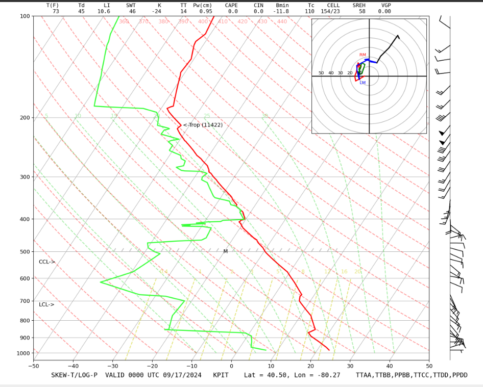
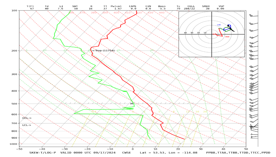
First, familiarize yourself with all of the lines. Look at a radiosonde ascent [8], such as the one from the National Center for Atmospheric Research Research Applications Laboratory [9] (type of plot: GIF of skew-T). The atmospheric sounding lines are temperature (solid red line) and dewpoint temperature (solid green line). These lines are plotted on a grid that shows –lnp on the vertical axis (horizontal blue lines) and temperature on the horizontal axis (blue lines tilting up and to the right—which is where "skew" comes from). –lnp is used because it varies nearly linear with height and the skewing of the temperature lines allows soundings to be shown without going out of bounds of the graph.
Here [10] is a blank skew-T diagram that you can play with and practice on. The diagram has an electronic pen that allows you to draw on it. This diagram will be used in Practice Quiz 3-4 and Quiz 3-4, so become familiar with it.
Please also note the following:
- The dry adiabat is the same line as an isentrope (curved red dash lines tilting to the upper left).
- The water vapor mixing ratio is the saturation water vapor mixing ratio at the dewpoint temperature, Td, for each pressure level (gold dot-dash lines tilting to the upper right).
- In clear air, for air parcels moving vertically:
- air parcels move along the dry adiabat and the potential temperature remains constant, even if they contain moisture;
- the water vapor mixing ratio is constant (but notice that Td changes!);
- Td of an air parcel moving vertically (and adiabatically) is decreasing, but not as fast as T of that air parcel is decreasing.
- Eventually, an air parcel moving vertically (along the dry adiabat) will have a temperature and dewpoint temperature that are the same, thus saturated.
- At this altitude level, called the Lifting Condensation Level (LCL), the relative humidity = 100%, T = Td, w = ws, and e = es. At this pressure and temperature, a cloud forms. Actually, the formation of a cloud requires a relative humidity that exceeds 100% by a few tenths of a percent, but we generally use 100% for the skew-T calculations. We will see why this extra relative humidity is necessary in the next lesson.
See the video below (1:19) for further explanation:
Moist Adiabat
When the air parcel is in a cloud, ascent causes a temperature decrease while the air remains saturated (i.e., w = ws, RH = 100%). Since ws decreases, the amount of water in the vapor phase decreases while the amount in the liquid or solid phase increases, but the total amount of water is constant (unless it rains!). As water vapor condenses, energy is released into the air and warms it a little bit. Thus, the lapse rate of the moist adiabat (curved dot-long-dash green lines tilting toward the upper left) is less than the lapse rate of the dry adiabat (9.8 K/km).
As long as it doesn’t rain or snow, an air parcel will move up and down a moist adiabat as long as it is in a cloud and will move up and down a dry adiabat when w < ws below the LCL.
- Once a cloud forms, any further rise of the air parcel will follow the moist adiabat (condensation of water vapor heats the air so that the temperature decrease with height is less than that of the dry adiabat). As long as the ascent is in the cloud, the relative humidity will remain near 100% and w = ws(T). Since T decreases on ascent, ws decreases, and more water goes into the liquid or ice phase.
- If the air parcel, containing the liquid or ice that was formed, descends, it will move along the moist adiabat until it again reaches the LCL, at which point all of the liquid water or ice will have evaporated or sublimed. Just below the LCL, all of the water will be vapor and the air parcel will descend along the dry adiabat and the water vapor mixing ratio will be constant.
The following is a summary for air parcel ascent and descent:
- From the initial p, T, and Td (or w), locate two points on the skew-T: (1) p and T and (2) p and Td (or w).
- Starting at the first point, move the parcel up the dry adiabat.
- Starting at the second point, move the parcel up the constant-w line. Note that Td is continually changing, so use w.
- Where the two lines intersect is the LCL.
- A cloud will form.
- If the air parcel continues to rise inside the cloud,
- w will always equal ws.
- the air parcel will follow the moist adiabat.
- If the parcel then descends,
- it will follow the moist adiabat down to the LCL.
- it will follow the dry adiabat below that.
- w will follow the w line below that.
The following video (1:43) discusses the process of adiabatic cooling and heating.
Other Potential Temperatures
There are other potential temperatures that are useful because they are conserved in certain situations and therefore can help you understand what the atmosphere is doing and what an air parcel is likely to do.
Virtual Potential Temperature
Virtual potential temperature is the potential temperature of virtual temperature, where density differences caused by water vapor are taken into account in the virtual temperature by figuring out the temperature of dry air that would have the same density:
This quantity is useful when comparing the potential temperatures (and thus densities) of air parcels at different pressures.
Wet Bulb Potential Temperature
The wet-bulb temperature is the temperature a volume of air would have if it were cooled adiabatically while maintaining saturation by liquid water; all the latent heat is supplied by the air parcel so that the air parcel temperature, when it descends to 1000 hPa, is less than its temperature would be had it descended down the dry adiabat.
The wet bulb temperature at any given pressure level is found by finding the LCL and then bringing the parcel up or down to the desired pressure level on the moist adiabat.
The wet bulb potential temperature, Θw, is the wet bulb temperature at p = 1000 hPa.
How can we use the wet bulb potential temperature? The wet bulb potential temperature is conserved, meaning it does not change, when an air mass undergoes an adiabatic process, such as adiabatic uplift or descent. If we consider large air masses that acquire similar temperature and humidity, then this entire air mass can take on the same wet bulb potential temperature. Colder, drier air masses will have a lower Θw. The Θw of this air mass can change if a diabatic process occurs, such as the warming of a cold air mass as it moves over warmer land, or the cooling of an air mass by radiating to space during the night, but these processes can sometimes take days. So an 850-mb map of Θw is one indicator of air masses and the fronts between air masses.
See the video below (:32) for further explanation:
Equivalent Potential Temperature
The equivalent potential temperature is the temperature that an air parcel would have if it were lifted adiabatically until all of the vapor were condensed and removed, and then brought to 1000 hPa adiabatically. For example, let's say you have an air parcel with some water vapor in it below the LCL. To find the equivalent potential temperature, you would (1) lift the parcel to the LCL along a dry adiabat, (2) lift the parcel along the moist adiabat all the way to the stratosphere so that all the water vapor condensed into liquid, and (3) bring the parcel down to 1000 hPa along the dry adiabat. Equivalent potential temperature accounts for the effects of condensation or evaporation on the change in the air parcel temperature.
Every 1 g/kg (g water vapor to kg of dry air) causes Θe to increase about 2.5 K. So, a moist air parcel with w = 10 g kg-1, which is not uncommon, will have Θe that is 25 K greater than Θ.
Approximately,
where Θ is the potential temperature, lv is the latent heat of vaporization, w is the water vapor mixing ratio, and cp is the specific heat capacity at constant pressure.
How can we use the equivalent potential temperature? The equivalent potential temperature, Θe is conserved when an air parcel or air mass undergoes an adiabatic process, just like the wet bulb potential temperature, Θw, is. Note also the total amount of water in vapor, liquid, and ice form is also conserved during adiabatic processes. The total amount of water is quantified using the total water mixing ratio, wt, which is defined in the same way that the water vapor mixing ratio (w) is defined except that it also includes liquid and solid water in the numerator. So, if we look at Θe and wt, we can learn a lot about the history of an air parcel. These conserved quantities are very useful to understand the history of air parcels around clouds. For example, if Θe changes but wt is constant, then the air parcel was either heated or cooled by a non-adiabatic process. On the other hand, if both Θe and wt change proportionally, then two air parcels with different initial values for Θe and wt have mixed. On a larger, more synoptic scale, gradients in Θe can be used to indicate the presence of fronts.
Another use of Θe is as an indicator of unstable air. Air parcels that have higher Θe tend to be unstable. Thus regions of high-Θe air are regions where thunderstorms might form if the surface heating is great enough to erase a temperature inversion.
See the video (1:01) below for further explanation:
Quiz 3-4: Using the skew-T.
- Find Practice Quiz 3-4 in Canvas. You may complete this practice quiz as many times as you want. It is not graded, but it allows you to check your level of preparedness before taking the graded quiz.
- When you feel you are ready, take Quiz 3-4. You will be allowed to take this quiz only once. Good luck!
3.6 Understanding the Atmosphere’s Temperature Profile
3.6 Understanding the Atmosphere’s Temperature Profile
Now we can begin to understand the reasons for the troposphere’s typical temperature profile. The atmosphere is mostly transparent to the incoming solar visible radiation, so Earth’s surface warms, and thus warms and moistens the air above it. This warm, moist air initially rises dry adiabatically, and then moist adiabatically once a cloud forms. Different air masses with different histories and different amounts of water mix and the result is a typical tropospheric temperature profile that has a lapse rate of (5–8) K km-1.
If atmospheric temperature profiles were determined only by atmospheric moisture, drier air masses would have lapse rates that are more like the dry adiabatic lapse rate, in which case we would expect that the skies would have fewer, thinner clouds. Moister air masses would have lapse rates that are closer to the moist adiabatic lapse rate, resulting in a sky filled with clouds at many altitudes.
But many processes affect the temperature of air at different altitudes, including mixing of air parcels, sometimes even from the stratosphere, and rain and evaporation of rain. Exchange of infrared radiation between Earth’s surface, clouds, and IR-absorbing gases (i.e., water vapor and carbon dioxide) also plays a major role in determining the atmosphere’s temperature profile, as we will show in the lesson on atmospheric radiation.The resulting atmospheric profiles can have local lapse rates that can be anywhere from less than the dry adiabatic lapse rate to greater than the moist adiabatic lapse rate. Look carefully at the temperature profile below. You will see evidence of many of these processes combining to make the temperature profile what it is.
If we average together all of these profiles over the whole year and over the whole globe, we can come up with a typical tropospheric temperature profile. According to the International Civil Aviation Organization (Doc 7488-CD, 1993), the standard atmosphere has a temperature of 15 oC at the surface, a lapse rate of 6.5 oC km–1 from 0 km to 11 km, a zero lapse rate from 11 km to 20 km, and a lapse rate of –1 oC km–1 from 20 km to 32 km in the stratosphere (i.e., temperature increases with height). Even though this standard profile is a good representation of a globally averaged profile, it is unlikely that such a temperature profile was ever seen with a radiosonde.
Combining knowledge of stability along with the knowledge of moist processes enables us to understand the behavior of clouds in the atmosphere. The following picture of water vapor released from a cooling tower at the Three-Mile Island nuclear reactor near Harrisburg, PA shows the water vapor quickly condensing to form a cloud. The cloud ascends, but then reaches a level at which its density matches the density of the surrounding air, the Equilibrium Level (EL). It still has kinetic energy, so keeps rising but increasingly slowly as its density becomes greater and greater than its surroundings. It then descends again, oscillating about the equilibrium level until it eventually settles there. The cloud then begins to spread out.

Summary and Final Tasks
Summary and Final Tasks
Water vapor is a key atmospheric constituent that is essential for weather. There are many ways to express and measure the amount of atmospheric water vapor—specific humidity, water vapor mixing ratio, partial pressure, relative humidity, and dewpoint temperature—and these are all related and can be used interchangeably, although some provide more physical insight than others depending on the question being asked. Water’s most important characteristic in the atmosphere is that it can change phases between vapor, liquid, and ice. In the atmosphere, water is either in the vapor phase or trying to establish an equilibrium between vapor and liquid or vapor and ice. The equilibria conditions are given by the Clausius–Clapeyron equation, which shows that the equilibrium (a.k.a. saturation) water vapor pressure depends only on the temperature. Water phase changes pack a big energy punch and drive weather events. We can calculate the atmospheric temperature changes resulting from phase changes and then see that these temperature changes greatly affect the buoyancy of air parcels and therefore their vertical motion.
A good way to visualize atmospheric vertical structure and behavior is the skew-T diagram. With it, we can readily deduce atmospheric properties and predict what weather is likely to happen if solar heating causes some air near the surface to ascend. Some of the most important properties found using the soundings on the skew-T are the lifting condensation level, the potential temperature, and the equivalent potential temperature. The behavior of a typical sounding on the skew-T shows that the troposphere’s thermal structure is caused in large part by adiabatic ascent and descent, although we will see later that absorption and emission of infrared radiation by water vapor and carbon dioxide also have a hand in shaping the temperature vertical profile.
Reminder - Complete all of the Lesson 3 tasks!
You have reached the end of Lesson 3! Make sure you have completed all of the activities before you begin Lesson 4.