Overview

The atmosphere is composed of billions of billions of molecules, 10⁴³ molecules to be exact. Each molecule is zooming at hundreds of meters per second but colliding with other molecules each billionth of a second, exchanging kinetic energy (½ mv²), momentum (mv), and internal energy (rotations and vibrations). It’s impossible to calculate what all of these molecules will do, so instead we study the energy and energy changes of volumes of molecules and use this information in our forecast models. This study is called thermodynamics. Thermodynamics has some difficult concepts to master, but it is also part of your everyday experience. In this lesson, you will learn the fundamental laws of thermodynamics and see how they describe our atmosphere’s pressure and temperature structure. You will learn why the atmosphere is sometimes stable and what happens when it isn’t.

Learning Objectives

By the end of this lesson, you should be able to:

use the fundamental gas laws - Ideal Gas Law, Dalton’s Law – to determine the relative densities of different air masses
derive the hydrostatic equilibrium equation from force balance to show why atmospheric pressure decreases with height
use the 1st Law of Thermodynamics and conservation of energy (i.e., adiabatic processes) to explain air parcel temperature changes
determine stability for different dry environmental temperature profiles
calculate buoyancy and vertical velocity with time

Questions?

If you have any questions, please post them to the Course Questions discussion forum. I will check that discussion forum daily to respond. While you are there, feel free to post your own responses if you, too, are able to help out a classmate.

2.1 Gas Laws

Understanding atmospheric thermodynamics begins with the gas laws that you learned in chemistry. Because these laws are so important, we will review them again here and put them in forms that are particularly useful for atmospheric science. You will want to memorize these laws because they will be used again and again in many other areas of atmospheric science, including cloud physics, atmospheric structure, dynamics, radiation, boundary layer, and even forecasting.

weather balloon floating above earth in space

A constant pressure balloon stays aloft for weeks at an altitude of 100,000 ft so that the instruments in the attached gondola can make long-term measurements.

Credit: Credit: Super Pressure Balloon. National Aeronautics and Space Administration [1] (NASA) (Public Domain)

Looking Ahead

Before you begin this lesson's reading, I would like to remind you of the discussion activity for this lesson. This week's discussion activity will ask you to take what you learn throughout the lesson to answer an atmospheric problem. You will not need to post your discussion response until you have read the whole lesson, but keep the question in mind as you read:

This week's topic is a hypothetical question involving stability. The troposphere always has a capping temperature inversion—it's called the stratosphere. The tropopause is about 16 km high in the tropics and lowers to about 10 km at high latitudes. The stratosphere exists because solar ultraviolet light makes ozone and then a few percent of the solar radiation is absorbed by stratospheric ozone, heating the air and causing the inversion. Suppose that there was no ozone layer and hence no stratosphere caused by solar UV heating of ozone.

Would storms in the troposphere be different if there was no stratosphere to act like a capping inversion? And if so, how?

You will use what you have learned in this lesson about the atmosphere's pressure structure and stability to help you to think about this problem and to formulate your answer and discussions. So, think about this question as you read through the lesson. You'll have a chance to submit your response in 2.6!

Ideal Gas Law

The atmosphere is a mixture of gases that can be compressed or expanded in a way that obeys the Ideal Gas Law:

$p V = N R^{*} T$

[2.1]

where p is pressure (Pa = kg m^–1 s^–2), V is the volume (m³), N is the number of moles, R* is the gas constant (8.314 J K^–1 mole^–1), and T is the temperature (K). Note also that both sides of the Ideal Gas Law equation have the dimension of energy (J = kg m² s^–2).

Recall that a mole is 6.02 x 10²³ molecules (Avogadro’s Number). Equation 2.1 is a form of the ideal gas law that is independent of the type of molecule or mixture of molecules. A mole is a mole no matter its type. The video below (6:17) provides a brief review of the Ideal Gas Law. Note that the notation in the video differs slightly from our notation by using n for N, P for p, and R for R*.

Ideal Gas Law Introduction

Credit: DeWitt, Tyler [2]. "Ideal Gas Law Introduction." YouTube. December 13, 2010.

Click here for transcript of the Ideal gas Law Introduction video.

So here I have a tank filled with gas. And these little dots represent some of the gas particles that would be in this tank. The arrows I put in here because all of these particles are in constant random motion. They're like a bunch of hyperactive little kids, running into each other all the time, banging into the sides of the container, and so forth. So we've got this tank of gas. Let's think about the characteristics that we could use to describe it. So one of the things that we could do is we could say what its temperature is. The higher the temperature, remember, the faster these gas particles are moving around, so temperature is very important when we talk about gas. Temperature for gases should always be reported in Kelvin. So we could say, for example, that the temperature of this guy here is 313 Kelvin. That's how hot these gas particles in the sample are. When you talk about gas, another important characteristic is pressure. How hard are these gas particles bouncing against the sides of the tank? How much pressure are they exerting on them? And we could measure these with a pressure gauge or something like that on the top of this tank. We could say, the pressure for this is 3.18 atm. That might be a pressure. And another thing that we spend a lot of time talking about when it comes to gas is volume. And again, I have these letters here that are how each one of these things are abbreviated. Volume, V, volume of this tank might be something like 95.2 liters. And finally, look at these particles that I've drawn. There is a certain amount of gas that's in here. And the amount of gas, which is abbreviated by the little letter n, is usually reported in moles, which is a convenient measure of how much of something we have. So we could say that the amount of gas in this tank is 7.5 moles. Now, whenever we have a sample of gas like this, if it's a tank or it's in a balloon or wherever it is, we can describe-- we can give it these various characteristics. And it turns out that also, for any sample of gas, if we know three of these characteristics, we can figure out what the fourth is. All we need to do is know three. And in order to do that, we use an equation that's a representation of the Ideal Gas Law. And it's written as P times V, pressure times volume, equals n, the amount of gas, times R times T, temperature. I'll get to R in a second. Don't worry about it for right now. It's going to be a number that we know. So let's say, for example, that we didn't know what pressure was, but we still knew the temperature, volume, and the amount of gas. No big deal. We could take the equation, PV equals nRT, and rearrange it. Divide both sides by V. Get rid of the V. And then we'd have P equals nRT divided by V. Plug these values in, and we could figure out what the pressure was. Or let's say that we knew what the pressure was of a particular gas sample. We know what the temperature was in a volume. But we didn't know what the amount of gas was. We don't know how much we had. We could figure out that fourth characteristic by rearranging the Ideal Gas Law for n, canceling out R and T on one side, rearranging it to solve for n. And then we could plug in the pressure, the volume, and the temperature, and we could figure out the amount of gas. So in other words, if we know three of these characteristics, we can always figure out what the fourth is. So you may be asking yourself, so R-- what's R? R is what we call a constant. It's a number that we know ahead of time that doesn't depend on the variables in our problem. The R that I'm going to be using most of the time for the videos is 0.0821 liters times atm divided by Kelvin times moles. Now notice that this is a fraction. It has both a top and a bottom. And it also is not just a number, but it has units. And check this out-- the units on R match the units in my problem. They match the characteristics that I'd be using. So I have liters here, liters here, atm, atm, Kelvin, Kelvin, and moles, moles. You always want the units on R to match the units of the characteristics in your Ideal Gas Problem. So because you always want the units to match, there are also different values of R, although I'm going to be using this mostly for the videos I'm doing. For example, let's say that instead of atm, I was using a pressure that was in millimeters of mercury. In this case, I wouldn't want to use this R here. I'd want to use this R here, so that the units match-- millimeters of mercury here, millimeters of mercury here, and the number's different-- 62.4. So again, that's what I use here. Let's say that instead of millimeters of mercury, my pressure was given to me in kPa. I would then use this value of R so that the units match. I've got kPa here, kPa here, and all the others are the same, so 8.31 for that. Now as I keep saying, in most of the videos that I'm going to be doing, I'm going to be using this top R with atm. But you may be asked by your teacher to use a different R. It's no big deal. That's probably just because they're giving you problems that have different pressure units, and they want the pressure units to match. So don't worry at all if you're using one of these other R's. Setting up and solving the Ideal Gas Law is exactly the same. No matter which of these R's you use, it's just a matter of plugging a different R in at the very end. So no matter which one you're using, you should be able to follow all these lessons, and it should all make sense.

Usually in the atmosphere we do not know the exact volume of an air parcel or air mass. To solve this problem, we can rewrite the Ideal Gas Law in a different useful form if we divide N by V and then multiply by the average mass per mole of air to get the mass density:

$ρ = \frac{N M}{V}$

[2.2]

where M is the molar mass (kg mol^–1). Density has SI units of kg m^–3. The Greek symbol ρ (rho) is used for density and should not be confused with the symbol for pressure, p.

Thus we can put density in the Ideal Gas Law:

$p = \frac{ρ R^{*} T}{M} o r ρ = \frac{M p}{R^{*} T}$

[2.3]

Density is an incredibly important quantity in meteorology. Air that is more dense than its surroundings (often called its environment) sinks, while air that is less dense than its surroundings rises. Note that density depends on temperature, pressure, and the average molar mass of the air parcel. The average molar mass depends on the atmospheric composition and is just the sum of the mole fraction of each type of molecule times the molar mass of each molecular constituent:

$M_{a v e r a g e} = \frac{\sum_{i} N_{i} M_{i}}{\sum_{i} N_{i}} = \frac{\sum_{i} N_{i} M_{i}}{N} = \sum_{i} \frac{N_{i}}{N} M_{i} = \sum_{i} f_{i} M_{i}$

[2.4]

where the i subscript represents atmospheric components, N is the number of moles, M is the molar mass, and f is the mole fraction. This video (3:19) shows you how to find the gas density using the Ideal Gas Law. You will note that the person uses pressure in kPa and molar mass in g/mol. Since kPa = 1000 Pa and g = 1/1000 kg, the two factors of 1000 cancel when he multiplies them together and he can get away with using these units. I recommend always converting to SI units to avoid confusion. Also, note that the symbol for density used in the video is d, which is different from what we have used (ρ, the convention in atmospheric science).

Find the Density of a Gas

Credit: ChemistNATE [3], "Find the Density of a Gas (Ideal Gas Law)." YouTube. March 13, 2013.

Click here for transcript of the Find the Density of a Gas video.

Solve the following problem on your own. After arriving at your own answer, click on the link to check your work.

Example

Let’s calculate the density of dry air where you live. We will use the Ideal Gas Law and account for the three most abundant gases in the atmosphere: nitrogen, oxygen, and argon. The mole fractions of the gases are 0.78, 0.21, and 0.01, respectively. M is the molar mass of air; M = 0.029 kg mol^–1, which is just an average that accounts for the mole fractions of the three gases:

\begin{array}{l} M = 0.78 M_{N}_{2} + 0.21 M_{O}_{2} + 0.01 M_{A}_{r} \\ = 0.78 \cdot 0.028 + 0.21 \cdot .032 + 0.01 \cdot 0.040 = 0.029 k g m o l^{- 1} \end{array}

R* = 8.314 J K^–1 mol^–1. Here, p = 960 hPa = 9.6 x 10⁴ Pa and T = 20 ^oC = 293 K.

Click for answer.

What would the density be if the room were filled with helium and not dry air at the same pressure and temperature?

Click for answer.

Dry Air

Often in meteorology we use mass-specific gas laws so that we must specify the gas that we are talking about, usually only dry air (N₂ + O₂ + Ar + CO₂ +…) or water vapor (gaseous H₂O). We can divide R^* by M_i to get a mass-specific gas constant, such as R_d = R*/M_{dry air}.

Thus, we will use the following form of the Ideal Gas Law for dry air:

$p_{d} = ρ_{d} R_{d} T$

[2.5]

where:

$R_{d} = \frac{R *}{M_{d r y a i r}} = \frac{8.314 {JK}^{- 1} {mol}^{- 1}}{0.02897 {kgmol}^{- 1}} = 287 m^{2} s^{- 2} K^{- 1} = 287 {Jkg}^{- 1} K^{- 1}$ .

M_{dry air} is 0.02897 kg mol^–1, which is the average of the molar masses of the gases in a dry atmosphere computed to four significant figures.

Note that p must be in Pascals (Pa), which is 1/100th of a mb (a.k.a, hPa), and T must be in Kelvin (K).

Water Vapor

We can do the same procedure for water vapor:

$p_{v} \equiv e = ρ_{v} R_{v} T$

[2.6]

where $R_{v} = \frac{R *}{M_{w a t e r v a p o r}} = \frac{8.314 {JK}^{- 1} {mol}^{- 1}}{0.01802 {kgmol}^{- 1}} = 461 m^{2} s^{- 2} K^{- 1} = 461 {Jkg}^{- 1} K^{- 1}$ .

Typically e is used to denote the water vapor pressure, which is also called the water vapor partial pressure.

Dalton’s Law

John Dalton

Credit: Dalton John desk [4] by H. Roscoe, W.H. Worthington, and J. Allen from Wikimedia [5] Public Domain [6]

This gas law is used often in meteorology. Applied to the atmosphere, it says that the total pressure is the sum of the partial pressures for dry air and water vapor:

$p = p_{d} + p_{H 2 O} = p_{d} + e$

[2.7]

Imagine that we put moist air and an absorbent in a jar and screw the lid on the jar. If we keep the temperature constant as the absorbent pulls water vapor out of the air, the pressure inside the jar will drop to p_d. Always keep in mind that when we measure pressure in the atmosphere, we are measuring the total pressure, which includes the partial pressures of dry air and water vapor.

So it follows that the density of dry air and water vapor also add:

$ρ = ρ_{d} + ρ_{v}$

[2.8]

Solve the following problem on your own. After arriving at your own answer, click on the link to check your work.

Check Your Understanding

Suppose we have two air parcels that are the same size and have the same pressure and temperature, but one is dry and the other is moist air. Which one is less dense?

Click for answer.

Virtual Temperature

Suppose there are two air parcels with different temperatures and water vapor amounts but the same pressure. Which one has a lower density? We can calculate the density to determine which one is lighter, but there is another way to do this comparison. Virtual temperature, T_v, is defined as the temperature dry air must have so that its density equals that of ambient moist air. Thus, virtual temperature is a property of the ambient moist air. Because the air density depends on the amount of moisture (for the same pressure and temperature), we have a hard time determining if the air parcel is more or less dense relative to its surroundings, which may have a different temperature and amount of water vapor. It is useful to pretend that the moist parcel is a dry parcel and to account for the difference in density by determining the temperature that the dry parcel would need to have in order to have the same density as the moist air parcel.

We can define the amount of moisture in the air by a quantity called specific humidity, q:

$q = \frac{ρ_{v}}{ρ_{d} + ρ_{v}}$

[2.9]

We see that q is just the fraction of water vapor density relative to the total moist air density. Usually q is given in units of g of water vapor per kg of dry air, or g kg^–1.

Using the Ideal Gas Law and Dalton’s Law, we can derive the equation for virtual temperature:

$T_{v} = T [1 + 0.61 q]$

[2.10]

where T and T_v have units of Kelvin (not ^oC and certainly not ^oF!) and q must be unitless (e.g., kg kg^–1).

Note that moist air always has a higher virtual temperature than dry air that has the same temperature as the moist air because, as noted above, moist air is always less dense than dry air for the same temperature and pressure. Note also that for dry air, q = 0 and the virtual temperature is the same as the temperature.

Solve the following problem on your own. After arriving at your own answer, click on the link to check your work.

Check Your Understanding

Consider a blob of air (T_blob = 25^oC, q_blob = 10 g kg^–1) at the same pressure level as a surrounding environment (T_env = 26^oC and q_env = 1 g kg^–1). If the blob has a lower density than its environment, then it will rise. Does it rise?

Click for answer.

We will use equation 2.10. Remember to convert T from ^oC to K and q from g kg^–1 to kg kg^–1!

$\begin{array}{l} T_{v b l o b} = (25 + 273) [1 + 0.61 \cdot .010] = 299.8 K = 26.8 {}^{o}C \\ T_{v e n v} = (26 + 273) [1 + 0.61 \cdot .001] = 299.2 K = 26.2 {}^{o}C \end{array}$

We see that the blob is less dense than its environment and so will rise. This difference of 0.6 ^oC may seem small, but it makes a huge difference in upward motion.

The following are some mistakes that are commonly made in the above calculations:

not converting from ^oC to K:

$\begin{array}{l} T_{v b l o b} = (25) [1 + 0.61 \cdot .010] = 25.15 {}^{o}C \\ T_{v e n v} = (26) [1 + 0.61 \cdot .001] = 26.02 {}^{o}C \end{array}$

We calculate that T_vblob < T_venv, which is the wrong answer.

not converting q from g/kg to kg/kg:

$\begin{array}{l} T_{v b l o b} = (25 + 273) [1 + 0.61 \cdot 10] = 2115 K = 1842 {}^{o}C \\ T_{v e n v} = (26 + 273) [1 + 0.61 \cdot 1] = 481 K = 208 {}^{o}C \end{array}$

We calculate that T_vblob > T_venv, which is correct in this case, but the numbers are crazy! After you complete your calculations, if the numbers you get just don’t seem right—like these—then you know that you have made a mistake in the calculation. Go looking for the mistake. Don’t submit an answer that makes no sense.

Once we find T_v, we can easily find the density of a moist parcel by using equation 2.5, in which we substitute T_v for T. Thus,

$ρ = \frac{p}{R_{d} T_{v}}$

Quiz 2-1: What will that air parcel do?

This quiz will give you practice calculating the virtual temperature and density using the Excel workbook that you set up in the last lesson.

Go to Canvas and find Practice Quiz 2-1. You may complete this practice quiz as many times as you want. It is not graded, but it allows you to check your level of preparedness before taking the graded quiz. I strongly suggest that you enter the equations for density and for virtual temperature in your Excel worksheet and use them to do all your calculations of density and virtual temperature on both the practice quiz and the quiz.
When you feel you are ready, take Quiz 2-1. You will be allowed to take this quiz only once. This quiz is timed, so after you start, you will have a limited amount of time to complete it and submit it. Good luck!

2.2 The Atmosphere’s Pressure Structure: Hydrostatic Equilibrium

The atmosphere’s vertical pressure structure plays a critical role in weather and climate. We all know that pressure decreases with height, but do you know why?

cube showing forces that determine hydrostatic balance as described in the text below

Air parcel at rest with three forces in balance

The atmosphere’s basic pressure structure is determined by the hydrostatic balance of forces [7]. To a good approximation, every air parcel is acted on by three forces that are in balance, leading to no net force. Since they are in balance for any air parcel, the air can be assumed to be static or moving at a constant velocity.

There are 3 forces that determine hydrostatic balance:

One force is downwards (negative) onto the top of the cuboid from the pressure, p, of the fluid above it. It is, from the definition of pressure [8],

$F_{t o p} = - p_{t o p} A$

[2.11]
Similarly, the force on the volume element from the pressure of the fluid below pushing upwards (positive) is:

$F_{b o t t o m} = p_{b o t t o m} A$

[2.12]
Finally, the weight [9] of the volume element causes a force downwards. If the density [10] is ρ, the volume is V, which is simply the horizontal area A times the vertical height, Δz, and g the standard gravity [11], then:

$F_{w e i g h t} = - ρ V g = - ρ g A Δ z$

[2.13]

By balancing these forces, the total force on the fluid is:

$\sum F = F_{b o t t o m} + F_{t o p} + F_{w e i g h t} = p_{b o t t o m} A - p_{t o p} A - ρ gA Δ z$

[2.14]

This sum equals zero if the air's velocity is constant or zero. Dividing by A,

$0 = p_{b o t t o m} - p_{t o p} - ρ g Δ z$

[2.15]

or:

$p_{t o p} - p_{b o t t o m} = - ρ g Δ z$

[2.16]

P_top − P_bottom is a change in pressure, and Δz is the height of the volume element – a change in the distance above the ground. By saying these changes are infinitesimally [12] small, the equation can be written in differential [13] form, where dp is top pressure minus bottom pressure just as dz is top altitude minus bottom altitude.

$d p = - ρ g d z$

[2.17]

The result is the equation:

$\frac{d p}{d z} = - ρ g$

[2.18]

This equation is called the Hydrostatic Equation. See the video below (1:18) for further explanation:

Hydrostatic Equation

Click here for transcript of the Hydrostatic Equation video.

Using the Ideal Gas Law, we can replace ρ and get the equation for dry air:

$\frac{d p}{d z} = - g \frac{p}{R_{d} T} o r \frac{d p}{p} = - \frac{g}{R_{d} T} d z = - \frac{M g}{R^{*} T} d z$

[2.19]

We could integrate both sides to get the altitude dependence of p, but we can only do that if T is constant with height. It is not, but it does not vary by more than about ±20%. So, doing the integral,

$p = p_{o} e^{- \frac{z}{H}} w h e r e p_{o} = s u r f a c e p r e s s u r e a n d H = \frac{R^{*} \bar{T}}{M_{a i r} g}$

[2.20]

H is called a scale height because when z = H, we have p = p_oe^–1. If we use an average T of 250 K, with M_air = 0.029 kg mol^–1, then H = 7.3 km. The pressure at this height is about 360 hPa, close to the 300 mb surface that you have seen on the weather maps. Of course the forces are not always in hydrostatic balance and the pressure depends on temperature, thus the pressure changes from one location to another on a constant height surface.

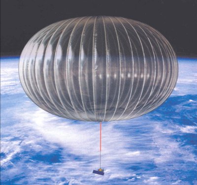
From equation 2.20, the atmospheric pressure falls off exponentially with height at a rate given by the scale height. Thus, for every 7 km increase in altitude, the pressure drops by about 2/3. At 40 km, the pressure is only a few tenths of a percent of the surface pressure. Similarly, the concentration of molecules is only a few tenths of a percent, and since molecules scatter sunlight, you can see in the picture below that the scattering is much greater near Earth's surface than it is high in the atmosphere.

Scattered light near Earth's surface.

Credit: NASA

Quiz 2-2: Harnessing the power of the hydrostatic equation

This quiz will give you practice using the hydrostatic equation to learn interesting and useful properties and quantities of the atmosphere.

I strongly suggest that you do all your calculations on this quiz using the Excel workbook.
There is no Practice Quiz 2-2. However, you have extra time to take this quiz.
When you feel you are ready, take Quiz 2-2 in Canvas. You will be allowed to take this quiz only once. This quiz is timed, so after you start, you will have a limited amount of time to complete it and submit it. Good luck!

2.3 First Law of Thermodynamics

Weather involves heating and cooling, rising air parcels and falling rain, thunderstorms and snow, freezing and thawing. All of this weather occurs according to the three laws of Thermodynamics. The First Law of Thermodynamics tells us how to account for energy in any molecular system, including the atmosphere. As we will see, the concept of temperature is tightly tied to the concept of energy, namely thermal energy, but they are not the same because there are other forms of energy that can be exchanged with thermal energy, such as mechanical energy or electrical energy. Each air parcel contains molecules that have internal energy, which when thinking about the atmosphere, is just the kinetic energy of the molecules (associated with molecular rotations and, in some cases, vibrations) and the potential energy of the molecules (associated with the attractive and repulsive forces between the molecules). Internal energy does not consider their chemical bonds nor the nuclear energy of the nucleus because these do not change during collisions between air molecules. Doing work on an air parcel involves either expanding it by increasing its volume or contracting it. In the atmosphere, as in any system of molecules, energy is not created or destroyed, but instead, it is conserved. We just need to keep track of where the energy comes from and where it goes.

Floating molecules

Credit: Ivana Vasilj via flickr

Let U be an air parcel’s internal energy, Q be the heating rate of that air parcel, and W be the rate that work is done on the air parcel. Then:

$\frac{d U}{d t} = Q + W$

[2.21]

The dimensions of energy are M L² T^–2 so the dimensions of this equation are M L² T^–3.

To give more meaning to this energy budget equation, we need to relate U, Q, and W to variables that we can measure. Once we do that, we can put this equation to work. To do this, we resort to the Ideal Gas Law.

For processes like those that occur in the atmosphere, we can relate working, W, to a change in volume because work is force times distance. Imagine a cylinder with a gas in it. The cross-sectional area of the piston is A. If the piston compresses the gas by moving a distance dx, the amount of work being done by the piston on the gas is the force (pA) multiplied by the distance (dx). W is then pAdx/dt. But the volume change is simply –Adx/dt and so:

$W = - p \frac{d V}{d t}$

[2.22]

Reducing a volume of gas (dV/dt < 0) takes energy, so working on an air parcel is positive when the volume is reduced, or dV/dt < 0. Thus:

$\frac{d U}{d t} = Q - p \frac{d V}{d t}$

[2.23]

Heat Capacity

The heat capacity C is the amount of energy needed to raise the temperature of a substance by a certain amount. Thus, $C = \frac{Q}{\frac{d T}{d t}}$ and has SI units of J/K. C depends on the substance itself, the mass of the substance, and the conditions under which the energy is added. We will consider two special conditions: constant volume and constant pressure.

Heat Capacity at Constant Volume

Consider a box with rigid walls and thus constant volume: $\frac{d V}{d T} = 0$ . No work is being done and only internal energy can change due to heating.

Heating a box with rigid walls.

Credit: W. Brune, after Verlinde

The candle supplies energy to the box, so Q > 0 and dU/dt > 0. The internal energy can increase via increases in molecular kinetic and potential energy. However, for an ideal gas, the attractive and repulsive forces between the molecules (and hence the molecular potential energy) can be ignored. Thus, the molecular kinetic energy and, hence, the temperature, must increase:

$\frac{d T}{d t} > 0$

[2.24]

So,

$Q_{\begin{matrix} c o n s t \\ v o l u m e \end{matrix}} = \frac{d U}{d t} = C_{V} \frac{d T}{d t}$

[2.25]

C_V, the constant relating Q to temperature change, is called the heat capacity at constant volume. Heat capacity has units of J K^-1.

Remember that $C_{v} \frac{d T}{d t}$ is the change in the air parcel’s internal energy.

The heat capacity, C_V, depends on the mass and the type of material. So we can write C_V as:

$C_{V} = m a s s \cdot c_{V}$

[2.26]

where c_V is called the specific heat capacity. The adjective “specific” means the amount of something per unit mass. The greater the heat capacity, the smaller the temperature change for a given amount of heating.

Some specific heat capacity values are included in the table below:

Specific Heat Capacity Values
gas	c_V (@ 0^oC) J kg^–1 K^–1
dry air	718
water vapor	1390
carbon dioxide	820

Solve the following problem on your own. After arriving at your own answer, click on the link to check your work.

Check Your Understanding

Consider a sealed vault with an internal volume of 10 m³ filled with dry air (p = 1013 hPa; T = 273 K). If the vault is being heated at a constant rate from the outside at a rate of 1 kW (1,000 J s^–1), how long will it take for the temperature to climb by 30 ^oC?

Click for answer.

The 1^stLaw can be rewritten as:

$Q = \frac{d U}{d t} + p \frac{d V}{d t} = C_{V} \frac{d T}{d t} + p \frac{d V}{d t} = m a s s \cdot c_{V} \frac{d T}{d t} + p \frac{d V}{d t}$

[2.27]

However, dV/dt = 0 because the vault’s volume isn’t changing. So, we can use the equation, rearrange it and integrate it:

$Q = m a s s \cdot c_{V} \frac{d T}{d t}$

[2.28]

How do we find the mass of the air inside the vault? Use the Ideal Gas Law to find the number of moles and then multiply by the mass per mole!

$m a s s = M_{d r y a i r} \cdot N = M_{d r y a i r} \cdot \frac{p V}{R^{*} T} = 0.029 \cdot \frac{1.013 x 10^{5} \cdot 10}{8.314 \cdot 273} = 12.9 k g$

$Δ t = \frac{m a s s \cdot c_{V} \cdot Δ T}{Q} = \frac{12.9 \cdot 718 \cdot 30}{10^{3}} = 278 s (~ 5 \min)$

Often we do not have a well-defined volume, but instead just an air mass. We can easily measure the air mass’s pressure and temperature, but we cannot easily measure its volume. Often we can figure out the heating rate per volume (or mass) of air. Thus:

$\frac{Q}{m a s s} \equiv q = \frac{m a s s \cdot c_{V} \frac{d T}{d t}}{m a s s} = c_{V} \frac{d T}{d t}; q = c_{V} \frac{d T}{d t}$

[2.29]

where q is the specific heating rate (SI units: J kg^–1 s^–1).

Heat Capacity Constant Pressure

The atmosphere is not a sealed box and when air is heated it can expand. We can no longer ignore the volume change. On the other hand, as the volume changes, any pressure changes are rapidly damped out, causing the pressure in an air parcel to be roughly constant even as the temperature and volume change. This constant-pressure process is called isobaric.

$Q = \frac{d U}{d t} + p \frac{d V}{d t}$

[2.30]

Now the change in the internal energy could be due to changes in temperature or changes in volume. It turns out that internal energy does not change with changes in volume. It only changes due to changes in temperature. But we already know how changes in internal energy are related to changes in temperature from the example of heating the closed box. That is, the internal energy changes are related by the heat capacity constant volume, C_v. Thus:

$Q = C_{V} \frac{d T}{d t} + p \frac{d V}{d t}$

[2.31]

Note that when volume is constant, we get the expression of heating a constant volume.

Suppose we pop the lid off the box and now the air parcel is open to the rest of the atmosphere. What happens when we heat the air parcel? How much does the temperature rise?

It’s hard to say because it is possible that the air parcel’s volume can change in addition to the temperature rise. So we might suspect that, for a fixed heating rate Q, the temperature rise in the open box will be less than the temperature rise in the sealed box where the volume is constant because the volume can change as well as the temperature.

Enthalpy

Enthalpy (H) is an energy quantity that accounts not only for internal energy but also the energy associated with working. It is a useful way to take into consideration both ways that energy can change in a collection of molecules – by internal energy changes and by volume changes that result in work being done.

$e n t h a l p y \equiv H = U + p V$

[2.32]

Enthalpy is the total energy of the air parcel including effects of volume changes. We can do some algebra and use the Chain Rule to write the First Law of Thermodynamics in terms of the enthalpy:

$Q = \frac{d U}{d t} + p \frac{d V}{d t} = \frac{d U}{d t} + \frac{d (p V)}{d t} - V \frac{d p}{d t} = \frac{d (U + p V)}{d t} - V \frac{d p}{d t} = \frac{d H}{d t} - V \frac{d p}{d t}$

[2.33]

If the pressure is constant, which is true for many air parcel processes, then dp/dt = 0 and:

$Q = \frac{d H}{d t}$

[2.34]

Summary

In a constant volume process, heating changes only the internal energy, U.
In a constant pressure process, heating changes enthalpy, H (both internal energy and working).

In analogy with constant volume process, for a constant pressure process, we can write:

$Q_{\begin{matrix} c o n s t a n t \\ p r e s s u r e \end{matrix}} = \frac{d H}{d t} = C_{p} \frac{d T}{d t}$

[2.35]

where C_p is the heat capacity at constant pressure and c_p is the specific heat capacity at constant pressure.

Note that c_p takes into account the energy required to increase the volume as well as to increase the internal energy and thus temperature.

What is the difference between c_p and c_v? You will see the derivation of the relationship, but I will just present the results:

by mole: $c_{(p, m)} = c_{(V, m)} + R^{*}$
by mass for dry air: $c_{p d} = c_{V d} + R_{d}$
by mass for water vapor: $c_{p v} = c_{V v} + R_{v}$

gas	c_V (@ 0^oC) J kg^–1 K^–1	c_p (@ 0^oC) J kg^–1 K^–1
dry air	718	1005
water vapor	1390	1858

Since c_p > c_v, the temperature change at constant pressure will be less than the temperature change at constant volume because some of the energy goes to increasing the volume as well as to increasing the temperature.

Summary of Forms of the First Law of Thermodynamics

$Q = C_{V} \frac{d T}{d t} + p \frac{d V}{d t}$

[2.36]

$Q = C_{p} \frac{d T}{d t} - V \frac{d p}{d t}$

[2.37]

$Q = \frac{d U}{d t} + p \frac{d V}{d t}$

[2.38]

$Q = \frac{d H}{d t} - V \frac{d p}{d t}$

[2.39]

It is often useful to express these equations in terms of specific quantities, such as specific volume (α ≡ V/m = ρ^-1), specific heat at constant pressure (c_p ≡ C_p/m), and specific heat at constant volume (c_V ≡ C_V/m). With these definitions, the first three equations above become:

$q = c_{V} \frac{d T}{d t} + p \frac{d α}{d t}$

[2.40]

$q = c_{p} \frac{d T}{d t} - α \frac{d p}{d t}$

[2.41]

$q = \frac{d u}{d t} + p \frac{d α}{d t}$

[2.42]

$q = \frac{d h}{d t} - α \frac{d p}{d t}$

[2.43]

You can figure out which form to use by following three steps:

Define the system. (i.e., what is the air parcel and what are its characteristics?)
Determine the process(es) (i.e., constant pressure, constant volume, heating, cooling?). Choose the form of the equation by making a term with a conserved quantity go away (i.e., dp/dt = 0 or dV/dt = 0) because then you have a simpler equation to deal with.
Look at which variables you have and then choose the equation that has those variables.

Check Your Understanding

Consider the atmospheric surface layer that is 100 m deep and has an average density of 1.2 kg m^–3. The early morning sun heats the surface, which heats the air with a heating rate of F = 50 W m^–2. How fast does the temperature in the layer increase? Why is this increase important?

What is the system? Air layer. Since we know the heating per unit area, work the problem per unit area.
What is the process? Constant pressure and heating by the sun.
Which variables do we have? $Q = C_{p} \frac{d T}{d t}$

Click for answer.

$Q = F A = 50 W m^{- 2} A$

$C_{p} = c_{p} ρ V = c_{p} ρ Δ z A$

$Q = F A = c_{p} ρ Δ z A \frac{d T}{d t}$

$\frac{d T}{d t} = \frac{F A}{c_{p} ρ Δ z A} = \frac{F}{c_{p} ρ Δ z} = \frac{50}{1005 1.2 100} = 4.2 x 10^{- 4} K s^{- 1} = 1.5 K h r^{- 1}$

This temperature increase is important because it is one of the most important factors in determining whether convection will occur later in the day. We will talk more about instability soon.

Here is a video (1:30) explanation of the above problem:

Dry Air Heating

Click here for transcript of the Dry Air Heating Video.

Check Your Understanding

Consider the atmospheric surface layer that is 100 m deep and has an average density of 1.2 kg m^–3. It is night and dark and the land in contact with the air is cooling at 50 W m^–2. If the temperature at the start of the night was 25 ^oC, what is the temperature 8 hours later?

What is the system? Air layer. Since we know the cooling per unit area, work the problem per unit area.
What is the process? Constant pressure and cooling by the land radiating energy to space and the air cooling by being in contact with the land.
Which variables do we have? $Q = C_{p} \frac{d T}{d t}$

Click for answer.

$Q = F A = -50 W m^{- 2} A$

$C_{p} = c_{p} ρ V = c_{p} ρ Δ z A$

$Q = F A = c_{p} ρ Δ z A \frac{d T}{d t}$

$\frac{d T}{d t} = \frac{F A}{c_{p} ρ Δ z A} = \frac{F}{c_{p} ρ Δ z} = \frac{-50}{1005 1.2 100} =- 4.2 x 10^{- 4} K s^{- 1} = -1.5 K h r^{- 1}$

Since the cooling continues for 8 hours, the total amount of cooling is –1.5 K/hr x 8 hr = 12 K or 12 ^oC. Thus, the temperature 8 hours later will be 13 ^oC.

This cooling near the surface creates a layer of cold air near the surface with a layer of warmer air above it. The layering of warm air over colder air creates an temperature inversion, which suppresses convection and lock pollutants into the air layer near Earth's surface.

2.4 The higher the temperature, the thicker the layer

A surprising way to relate the distance between two pressure surfaces to the temperature of the layer between them.

Consider a column of air between two pressure surfaces. If the mass in the column is conserved, then the column with the greater average temperature will be less dense and occupy more volume and thus be higher in altitude. But the pressure at the top of the column is related to the weight of the air above the column, which is constant, and so the upper pressure surface is higher in altitude. If the temperature of the column is lower, then the pressure surface at the top of the column will be lower in altitude.

We can look at this behavior from the point-of-view of hydrostatic equilibrium.

$\frac{d p}{d z} = - ρ g = - \frac{p g}{R_{d} T}$

If the temperature is greater, then the change in p with height is less, which means that any given pressure surface is going to be higher.

The difference between any two pressure surfaces is called the thickness.

We can show that the thickness depends only on temperature:

$d z = - \frac{d p}{p} \frac{R_{d}}{g} T$

Integrate both sides:

$\int_{z_{1}}^{z_{2}} d z =- \int_{p_{1}}^{p_{2}} \frac{d p}{p} \frac{R_{d}}{g} T$

or

$z_{2} - z_{1} = \frac{R_{d}}{g} ln (\frac{p_{1}}{p_{2}}) \bar{T}$

where T is the average temperature of the layer between p₁ and p₂. So, the thickness is actually a measure of the average temperature in the layer.

To Learn More

As some of you already know, you can use the thickness between different pressure surfaces to estimate the type of precipitation that will fall - snow, rain, or a mixture. You can check out these resources for some more information and example problems:

Weather Forecasting Online Review Questions [14]

Discussion of Thickness and its Uses [15]

Check Your Understanding

Suppose that the 500 mb surface is at 560 dam (decameters, 10s of meters) and the 1000 mb surface is at 0 dam. What is the average temperature of the layer between 1000 mb and 500 mb?

Click for answer.

Rearrange equation 2.4 to get an expression in terms of the average temperature and then put all the numbers into the equation to find the average temperature of the layer. Make sure that all the units are correct.

\bar{T} = \frac{10 * (z_{2} - z_{1})}{(\frac{287}{9.8}) \ln (\frac{p_{1}}{p_{2}})} = \frac{10 * (560 - 0)}{(\frac{287}{9.8}) \ln (\frac{1000}{500})} = 276 K

2.5 Adiabatic Processes: The Path of Least Resistance

Adiabatic Process

So far, we have covered constant volume (isochoric) and constant pressure (isobaric) processes. There is a third process that is very important in the atmosphere—the adiabatic process. Adiabatic means no energy exchange between the air parcel and its environment: Q = 0. Note: adiabatic is not the same as isothermal.

Consider the Ideal Gas Law:

$p V = n R^{*} T$

[2.1]

If an air parcel rises, the pressure changes, but how does the temperature change? Note that the volume can change as well as the pressure and temperature, and thus, if we specify a pressure change, we cannot find the temperature change unless we know how the volume changed. Without some other equation, we cannot say how much the temperature will rise for a pressure change.

as pressure changes, volume and temp change too. Pressure decreases with height

Changes in volume and temperature as an air parcel ascends and the pressure decreases.

Credit: W. Brune, after Lamb and Verlinde

However, we can use the First Law of Thermodynamics to relate changes in temperature to changes in pressure and volume for adiabatic processes.

Derivation of the Poisson Relations

I do not expect you to be able to do this derivation, but you should go through it to make sure that you understand all the steps as a way to continue to improve your math skills. Start with the following specific form of the 1^st Law for dry air (Equation 2.41) and then assume an adiabatic process (q = 0):

$q = c_{p} \frac{d T}{d t} - α \frac{d p}{d t}$

[2.45]

$q = 0 = c_{p} \frac{d T}{d t} - α \frac{d p}{d t}$

[2.46]

Divide both sides by T:

$\frac{c_{p}}{T} \frac{d T}{d t} - \frac{R_{d} T}{p T} \frac{d p}{d t} = 0 = \frac{c_{p}}{T} \frac{d T}{d t} - \frac{R_{d}}{p} \frac{d p}{d t} = c_{p} \frac{d l n (T)}{d t} - R_{d} \frac{d l n (p)}{d t}$

[2.47]

where we figured out the two terms were just derivatives of the natural log of T and p.

$\frac{d}{d t} (c_{p} l n (T) - R_{d} l n (p)) = 0$

[2.48]

But d/dt = 0 just means that the value is constant:

$(c_{p} l n (T) - R_{d} l n (p)) = c o n s t a n t$

[2.49]

Divide by c_p:

$l n (T) - \frac{R_{d}}{c_{p}} l n (p) = l n (T) + l n (p^{(\frac{- R_{d}}{c_{p}})}) = l n (T p^{(\frac{- R_{d}}{c_{p}})}) = c o n s t a n t$

[2.50]

If the natural log of a variable is constant then the variable itself must be constant:

$T p^{(\frac{- R_{d}}{c_{p}})} = c o n s t a n t$

[2.51]

We can rewrite R_d/c_p as a new term denoted by the Greek letter gamma, γ

$γ \equiv \frac{c_{p}}{c_{v}} = \frac{c_{v} + R_{d}}{c_{v}} = 1.4$

[2.52]

$\frac{R_{d}}{c_{p}} = \frac{γ - 1}{γ} = 0.286$

[2.53]

We can use the Ideal Gas Law to get relations among p, V, and T, called the Poisson’s Relations:

$T p^{(\frac{- R_{d}}{c_{p}})} = T p^{(\frac{(1 - γ)}{γ})} = c o n s t a n t$

[2.54]

$α^{γ} p = c o n s t a n t$

[2.55]

$T α^{γ - 1} = c o n s t a n t$

[2.56]

Potential Temperature

The Poisson Relation that we use the most is the relation of pressure and temperature because these are two variables that we can measure easily without having to define a volume of air:

$\frac{T}{θ} = {(\frac{p}{p_{o}})}^{(\frac{R_{d}}{c_{p}})}$

[2.57]

or

$θ = T {(\frac{p_{o}}{p})}^{\frac{R_{d}}{c_{p}}} = T {(\frac{1000}{p})}^{0.286}$

[2.58]

We call θ the potential temperature, which is the temperature that an air parcel would have if the air is brought to a pressure of p_o = 1000 hPa. Potential temperature is one of the most important thermodynamic quantities in meteorology.

Adiabatic processes are common in the atmosphere, especially the dry atmosphere. Also, adiabatic processes are often the same as isentropic processes (no change in entropy).

Check Your Understanding

Air coming over the Laurel Highlands descends from about 700 m (p ~ 932 hPa) to 300 m (p ~ 977 hPa) at State College. Assume that the temperature in the Laurel Highlands is 20 ^oC. What is the temperature in State College?

Click for answer.

We can find the temperature in State College due only to adiabatic changes by the following equation:

$\begin{array}{l} T_{7}_{00} p_{7} {_{00}}^{- 0.286} = T_{3}_{00} p_{3} {_{00}}^{- 0.286} \\ T_{300 =} T_{700} {(\frac{p_{300}}{p_{700}})}^{0.286} = (273 + 20) {(\frac{977}{932})}^{0.286} = 297 K = 24 C \end{array}$

This temperature change is 4 ^oC, or 7 ^oF just from adiabatic compression.

We can plot adiabatic (isentropic) surfaces in the atmosphere. An air parcel needs no energy to move along an adiabatic surface. Also, it takes energy for an air parcel to move from potential surface to another potential energy surface.

plot of adiabatic surfaces in the atmosphere as described in the text above. lines are further apart at higher pressures and lower latitudes

Potential temperature (solid lines, K) as a function of latitude and altitude. Note that the decrease in potential temperature with height is small in the troposphere and large in the stratosphere.

Credit: W. Brune, after Andews, Holton, and Leovy

Check Your Understanding

Suppose an air parcel has p = 300 hPa and T = 230 K. How much heating per unit volume of dry air would be needed to increase the potential temperature by 10 K?

Click for answer.

The heating raises the temperature, and the amount of heating required depends on the heat capacity, constant pressure, which depends on the mass of air, or the density times the volume. Let's do the calculation for a volume of air; that way we can use the density.

First we need to find the temperature rise that is the same as a potential temperature rise of 10 K at a pressure of 300 hPa.

$d θ = d T {(\frac{1000}{p})}^{0.286} d T = 10 {(\frac{300}{1000})}^{0.286} = 7.1 K$

Then we need to find the density so that we can calculate the heat capacity:

$ρ = \frac{p}{R_{d} T} = \frac{{3x10}^{4}}{287 \cdot 230} = 0.45 k g m^{- 3}$

Now we can put it all together:

$\frac{Q Δ T}{V} = \frac{ρ \cdot V \cdot c_{p} \cdot Δ T}{V} \Rightarrow \frac{Q Δ T}{V} = ρ \cdot c_{p} \cdot Δ T =0.45 \cdot 1005 \cdot 7.1 = 3.2 x 10^{3} J m^{- 3}$

Note that we were asked to provide the total heating per unit volume, which is just the heating rate times time divided by the unit volume. So the quantity on the left is what we want. Is this heating large? Yes! So it takes a lot of heating or cooling the raise or lower an air parcel potential temperature just 10 K.

Dry Adiabatic Lapse Rate

The temperature change with change in pressure (and thus change in altitude) is a major reason for weather. For dry air, the main effect is buoyancy. So because the pressure change generally follows the hydrostatic equation, the change in height translates into a change in pressure which translates into a change in temperature due to adiabatic expansion. Note that as the air parcel rises, its pressure quickly adjusts to the pressure of the surrounding air. Thus we can determine the dry adiabatic lapse rate by starting with the Poisson relation between pressure and temperature:

$T p^{(\frac{- R_{d}}{c_{p}})} = c o n s t a n t$

[2.59]

Take the derivative w.r.t. z:

$\frac{d T}{d z} p^{(\frac{- R_{d}}{c_{p}})} + T (\frac{- R_{d}}{c_{p}}) p^{(\frac{- R_{d}}{c_{p}}) - 1} \frac{d p}{d z} = \frac{d T}{d z} + T (\frac{- R_{d}}{c_{p}}) p^{- 1} \frac{d p}{d z} = 0$

[2.60]

But we also know from the hydrostatic equation that:

$\frac{d p}{d z} = - ρ g$

[2.18]

Substituting –ρg for dp/dz into the equation and rearranging the terms:

$\frac{d T}{d z} = T (\frac{- R_{d}}{c_{p}}) p^{- 1} ρ g = - T (\frac{R_{d}}{c_{p}}) p^{- 1} g (\frac{p}{R_{d} T})$

[2.61]

$$ -\frac{d T}{d z} \equiv \Gamma_{d}=\frac{g}{c_{p}}=\frac{9.8 \frac{m}{s^2}}{1005 J k g^{-1} K^{-1}}=9.8 K k m^{-1} $$

[2.62]

Γ_d is called the dry adiabatic lapse rate. Note that the temperature decreases with height, but the dry adiabatic lapse rate is defined as being positive.

Check Your Understanding

Air coming over the Laurel Highlands descends from about 700 m to 300 m at State College. Assume that the temperature in the Laurel Highlands is 20 ^oC. What is the temperature in State College?

Click for answer.

We can find the temperature in State College due only to adiabatic changes by using the dry adiabatic lapse rate multiplied by the height change:

$d T = - Γ_{d} (300 - 700) = 9.8 K k m^{- 1} \cdot 0.4 = 4^{\circ} C$

This temperature change is 4.0 ^oC, or 7 ^oF just from adiabatic compression. This answer is very similar to the answer we obtained using the change in potential temperature.

Quiz 2-3: Energy budgets and balance.

This quiz is practice calculating energy balance using the First Law of Thermodynamics. Some of the problems will involve potential temperature.

Go to Canvas and find Practice Quiz 2-3. You may complete this practice quiz as many times as you want. It is not graded, but it allows you to check your level of preparedness before taking the graded quiz.
When you feel you are ready, take Quiz 2-3. You will be allowed to take this quiz only once. This quiz is timed, so after you start, you will have a limited amount of time to complete it and submit it. Good luck!

2.6 Stability and Buoyancy

We know that an air parcel will rise relative to the surrounding air at the same pressure if the air parcel’s density is less than that of the surrounding air. The difference in density can be calculated using the virtual temperature, which takes into account the differences in specific humidity in the air parcel and the surrounding air as well as the temperature differences.

Stability

In equilibrium, the sum of forces are in balance and the air parcel will not move. The question is, what happens to the parcel if there is a slight perturbation in its vertical position?

Stable: Ball sits in a valley, Unstable: Ball sits at the top of a hill

Examples of instability (left) and stability (right).

Credit: W. Brune, after H. Verlinde

For the figure on the left, if the ball is displaced a tiny bit to the left or the right, it will be pulled by gravity and will continue to roll down the slope. That position is unstable. For the figure on the right, if the ball is displaced a little bit, it will be higher than the central position and gravity will pull it back down. It may rock back and forth a little bit, but eventually it will settle down into its original position.

To assess instability of air parcels in the atmosphere, we need to find out if moving the air parcel a small amount up or down causes the parcel to continue to rise or to fall (instability) or if the air parcel returns to its original position (stability).

Now look at some atmospheric temperature profiles. Important: a dry air parcel that is pushed from its equilibrium position always moves along the dry adiabatic lapse rate (DALR) line.

Unstable (left) & Stable (right). Left: Gamma(d) less than Gamma(env) Right: Gamma(d) more than Gamma(env). Gamma (env.) = -dT(env)/dz

Determining instability (left) and stability (right) of an air parcel by moving it on the DALR slope and seeing if the parcel’s temperature is greater or less than the environmental temperature.

Credit: W. Brune

Note that we can also show that if the air parcel is pushed down, it will keep going if the atmospheric (environmental) profile looks like the one on the left and will return to the original position if it looks like the one on the right.

graph with Alltitude on y-axis and temperature on x-axis. 4 DALR lines are show and a red line labeled atmospheric weaves through 5 points

An atmospheric temperature profile (red) and the movement of individual air parcels (numbered circles) along dry adiabats (dashed lines).

Credit: W. Brune

Check Your Understanding

Use the image above to determine the following:

Is the air parcel stable or unstable at each of the points, 1-5?

Click for answer.

Buoyancy

We can calculate the acceleration an unstable air parcel will have and, from this, can determine the parcel’s velocity at some later point in time. This acceleration is called buoyancy (B).

Cube with two downward forces and one upward force acting on it. see surrounding text

Forces on an air parcel that has a different density from its environment.

Credit: W. Brune

$\sum F = F_{b o t t o m} + F_{t o p} + F_{w e i g h t} = p_{b o t t o m} A - p_{t o p} A - ρ^{'} g A h$

[2.63]

Let’s look at the forces on an air parcel again, like we did to derive the hydrostatic equilibrium. But this time, let’s assume that the parcel has a different density than the surrounding air. We will designate quantities associated with the air parcel with an apostrophe (’); environmental parameters will have no superscript.

If the forces are not in balance, then we need to keep the acceleration that we set to zero in the hydrostatic equilibrium case. We can also divide both sides of the equation by the mass of the air parcel:

$\frac{\sum F}{ρ^{'} V} = \frac{- \frac{p_{t o p} - p_{b o t t o m}}{Δ z} - ρ^{'} g}{ρ^{'}} \to \frac{- (- ρ g) - ρ^{'} g}{ρ^{'}}$

[2.64]

$a \equiv B = \frac{(ρ - ρ^{'}) g}{ρ^{'}}$

[2.65]

where we have used the hydrostatic equilibrium of the environment to replace the expression for the pressure change as a function of height with the density times the acceleration due to gravity.

We can then use the Ideal Gas Law to replace densities with virtual temperatures because the pressure of the parcel and its surrounding air is the same:

$B = \frac{(\frac{1}{T_{v}} - \frac{1}{T_{v}^{'}}) g}{\frac{1}{T_{v}^{'}}} = \frac{(T_{v}^{'} - T_{v})}{T_{v}} g$

[2.66]

If B > 0, then the parcel accelerates upwards; if B < 0, then the parcel accelerates downwards.

We look at the instability at each point in the environmental temperature profile and can determine Γ_env for each point.

Thus,

$T_{e n v} = T_{0} + {\frac{\partial T}{\partial z} |}_{e n v} Δ z = T_{0} - Γ_{e n v} Δ z; T_{p a r c e l} = T_{0} + {\frac{\partial T}{\partial z} |}_{p a r c e l} Δ z = T_{0} - Γ_{d} Δ z;$

[2.67]

so that:

$B = \frac{(T_{0} - Γ_{d} Δ z - T_{0} + Γ_{e n v} Δ z)}{T_{v}} g = \frac{(Γ_{e n v} - Γ_{d})}{T_{v}} g Δ z$

[2.68]

If Γ_env < Γ_d, the parcel accelerates downward for positive Δz (statically stable environment).

If Γ_env > Γ_d, the parcel accelerates upward for positive Δz (statically unstable environment).

We can put this idea of buoyancy in terms of potential temperature.

$θ = T {(\frac{p_{o}}{p})}^{\frac{R_{d}}{c_{p}}}$

We want to find dθ/dz. Taking the log of both sides of the equation and replacing a dp/dz term with –gρ, we are able to find the following expression for buoyancy in terms of potential temperature:

$B = - g Δ z \frac{1}{θ} \frac{d θ}{d z}$

[2.69]

Remember that no matter what the environmental temperature or potential temperature profiles, a change in height of an air parcel will result in a temperature that changes along the dry adiabat and a potential temperature that does not change at all. As you can see below, the stability of a layer depends on the change in environmental potential temperature with height. Air parcels try to move vertically with constant potential temperature.

graph with theta on x and z on y. Graph shows central vertical section with two slopes moving towards the right from either end of the line

Layer stability for different profiles of potential temperature.

Credit: W. Brune

Parcels will move to an altitude (and air density) for which B = 0. However, if they still have a velocity when they reach that altitude, they will overshoot, experience a negative acceleration, and then descend, overshooting the neutral level again. In this way, the air parcel will oscillate until its oscillation is finally damped out by friction and dissipation of the air parcel. Note that in the neutral section of vertical profile where potential temperature does not change, it is not possible to determine if an air parcel will be stable or unstable. For instance, if the air parcel in the neutral region is given a small upward push, it will continue to rise until it reaches a stable region.

Quiz 2-4: Stability and buoyancy.

This quiz provides practice determining stability or instability of an air parcel and in calculating the buoyancy of air parcels.

Go to Canvas and find Practice Quiz 2-4. You may complete this practice quiz as many times as you want. It is not graded, but it allows you to check your level of preparedness before taking the graded quiz.
When you feel you are ready, take Quiz 2-4. You will be allowed to take this quiz only once. Good luck!

Discussion Forum 1: Storms in the troposphere

(3 discussion points)

This week's discussion topic is a hypothetical question involving stability. The troposphere always has a capping temperature inversion–it's called the stratosphere. The tropopause is about 16 km high in the tropics and lowers to about 10 km at high latitudes. The stratosphere exists because solar ultraviolet light makes ozone and then a few percent of the solar radiation is absorbed by stratospheric ozone, heating the air and causing the inversion. Suppose that there was no ozone layer and hence no stratosphere caused by solar UV heating of ozone.

Would storms in the troposphere be different if there were no stratosphere to act like a capping inversion? And if so, how?

Use what you have learned in this lesson about the atmosphere's pressure structure and stability to help you to think about this problem and to formulate your answer and discussions. It's okay to be wrong, as long as you have some solid reasoning to back up your ideas. My goal is to get you all to communicate with each other and think hard about atmospheric science.

You can access the Storms in the troposphere Discussion Forum in Canvas.
Post a response that answers the question above in a thoughtful manner that draws upon course material and outside sources.
Keep the conversation going! Comment on at least one other person's post. Your comment should include follow-up questions and/or analysis that might offer further evidence or reveal flaws.

This discussion will be worth 3 discussion points. I will use the following rubric to grade your participation:

Discussion Activity Grading Rubric
Evaluation	Explanation	Available Points
Not Completed	Student did not complete the assignment by the due date.	0
Student completed the activity with adequate thoroughness.	Student answers the discussion question in a thoughtful manner, including some integration of course material.	1
Student completed the activity with additional attention to defending their position.	Student thoroughly answers the discussion question and backs up reasoning with references to course content as well as outside sources.	2
Student completed a well-defended presentation of their position, and provided thoughtful analysis of at least one other student’s post.	In addition to a well-crafted and defended post, the student has also engaged in thoughtful analysis/commentary on at least one other student’s post as well.	3

Summary and Final Tasks

We started with the Ideal Gas Law and Dalton’s Law to develop an understanding of the atmosphere’s behavior and atmospheric density, a fundamental driving force for vertical motion in the atmosphere. We saw that composition matters, and developed a new quantity, virtual temperature, that allows us to compare the densities of different moist air parcels. Using these laws along with Newton’s laws, we were able to derive a fundamental property of the atmosphere: the hydrostatic equation, which states that the change in pressure with altitude is proportional to the negative of the density times gravity. We applied a new constraint – the First Law of Thermodynamics, which states that energy is conserved and saw that combining it with the gas laws enabled us to calculate temperature changes and to derive an important atmospheric quantity – the potential temperature. With these concepts, we were able to determine the stability (and instability) of an air parcel. We could also determine the buoyancy of an air parcel, which allows us to calculate the acceleration and thus the velocity of an air parcel after it has accelerated for a while.

Reminder - Complete all of the Lesson 2 tasks!

You have reached the end of Lesson 2! Be sure to complete the Activities within three days of the end of the lesson. I strongly encourage you to do them as you are going through the lesson.

Lesson 2: Thermodynamics

Overview

Overview

Learning Objectives

Questions?

2.1 Gas Laws

2.1 Gas Laws

Looking Ahead

Ideal Gas Law

Example

Dry Air

Water Vapor

Dalton’s Law

Check Your Understanding

Virtual Temperature

Check Your Understanding

Quiz 2-1: What will that air parcel do?

2.2 The Atmosphere’s Pressure Structure: Hydrostatic Equilibrium

2.2 The Atmosphere’s Pressure Structure: Hydrostatic Equilibrium

Quiz 2-2: Harnessing the power of the hydrostatic equation

2.3 First Law of Thermodynamics

2.3 First Law of Thermodynamics

Heat Capacity

Heat Capacity at Constant Volume

Check Your Understanding

Heat Capacity Constant Pressure

Enthalpy

Summary

Summary of Forms of the First Law of Thermodynamics

Check Your Understanding

Check Your Understanding

2.4 The higher the temperature, the thicker the layer

2.4 The higher the temperature, the thicker the layer

To Learn More

Check Your Understanding

2.5 Adiabatic Processes: The Path of Least Resistance

2.5 Adiabatic Processes: The Path of Least Resistance

Adiabatic Process

Derivation of the Poisson Relations

Potential Temperature

Check Your Understanding

Check Your Understanding

Dry Adiabatic Lapse Rate

Check Your Understanding

Quiz 2-3: Energy budgets and balance.

2.6 Stability and Buoyancy

2.6 Stability and Buoyancy

Stability

Check Your Understanding

Buoyancy

Quiz 2-4: Stability and buoyancy.

Discussion Forum 1: Storms in the troposphere

Summary and Final Tasks

Summary and Final Tasks

Reminder - Complete all of the Lesson 2 tasks!