Introduction to Multiple Linear Regression

Introduction to Multiple Linear Regression

Read It: Multiple Linear Regression

At its core, multiple linear regression is very similar to simple linear regression. Recall the equation for a simple linear model from Lesson 8: 

In this equation, we have a single explanatory variable (also known as a predictor), which is denoted with $X$. To define a multiple linear regression model, we maintain this same basic formula, but add more explanatory variables:

Notice that we do not include multiple X values (e.g., $X\mathrm{\_}1,X\mathrm{\_}2,\dots ,X\mathrm{\_}k$) to indicate the multiple explanatory variables included in the model.

Another similarity between simple linear regression and multiple linear regression are the conditions that need to be met for statistical validity. Recall from Lesson 8, the three conditions for simple linear regression are: (a) linear shape, (b) constant variance, and (c) no outliers. Multiple linear regression has the same conditions, except we test them by plotting the predicted values vs. the residuals, as shown below. 

Conditions that break assumptions of the simple linear model

Credit: © Penn State is licensed under CC BY-NC-SA 4.0

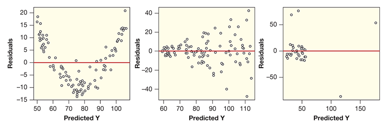
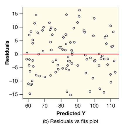
Notice, for example, the curved shape between the predicted Y values and the residuals in Figure (a), this is an indication that there is a nonlinear relationship, which breaks the conditions for multiple linear regression. Likewise, in Figure (b), there is a clear fan or wedge shape between the predicted Y values and the residuals, which breaks the constant variance condition. Finally, in Figure (c), there are clear outliers, which breaks the no outliers condition. Below, we show the ideal plot of predicted Y values vs. residuals, in which none of the conditions are broken. 

Ideal plot of predicted Y values vs. residuals

Credit: © Penn State is licensed under CC BY-NC-SA 4.0

You may have noticed that all of these plots are working with the predicted Y values, rather than the actual values. This means that we can only assess the validity of our multiple linear regression model after we actually implement the model. This is a particular limitation of multiple linear regression, as it can often we a lot of work to build the model, only to find out that it doesn't meet the statistical conditions. Nonetheless, the ability to include additional explanatory variables often improves our model, so it is generally a worthwhile endeavor to spend some time perfecting the multiple linear regression model.

 Assess It: Check Your Knowledge