Introduction to Decision Trees

Introduction to Decision Trees

Read It: Decision Trees

Recall from Lesson 10 the discussion about neural networks. Like neural networks, decision trees are a complex model that can be used to make predictions for nonlinear data. However, while neural networks were modeled after the human brain, decision trees are modeled after trees (as the name suggests). Another key difference is that we will discuss decision trees in terms of both classification and regression, while with neural networks, you focused on regression. Classification, like regression, makes a prediction about some data. However, that data is categorical, and the prediction focuses on which group or category a new data point gets placed into. 

A decision tree, therefore, can be used to classify categorical response variables based on a number of different explanatory variables. An advantage of decision trees is the ability to visualize the exact path a data point would take in order to be classified as a certain category. An example of a decision tree is shown below. Here, the goal of the model is to predict whether an individual will take a job, given a series of criteria. Each of these criteria is framed as a yes/no condition. That is, the criteria pose questions for which a “yes” answer will move along a different path than a “no” answer. The closer these criteria are to the top of the tree, the more important that choice. In the figure below, for example, the salary is the most important criterion for accepting a new job, so it is the first decision that needs to be made in the tree. If the answer to the question ("is the salary greater than $50,000") is “yes”, the data point (i.e., the job offer) moves along the left side of the tree; otherwise, the data point moves to the right and stops at a final node that classified the job offer as “decline”. 

Enter caption here
Credit: rashida048. “Simple Explanation on How Decision Tree Algorithm Makes Decisions.” Regenerative Today. April 7, 2022.

There are some key terms associated with decision trees.

In terms of the mechanics behind developing decision trees, the splits are chosen based on the importance, often measured by how “good” an individual split is at separating categories. These splits are recursive, meaning that they are repeated to create smaller and smaller boxes until all the data points are successfully classified. Below, we show an animation of how this splitting might work. Imagine you have a categorical response variable and two explanatory variables, x and y. The first split will find the point along the x-axis that best categorizes the data and draws the line δ. Then, in the next round, the model finds the best point on the y-axis to further categorize the data and draws the line γ. This continues as the model creates smaller boxes. A stopping condition is usually in place to stop the model and speed up the model. 

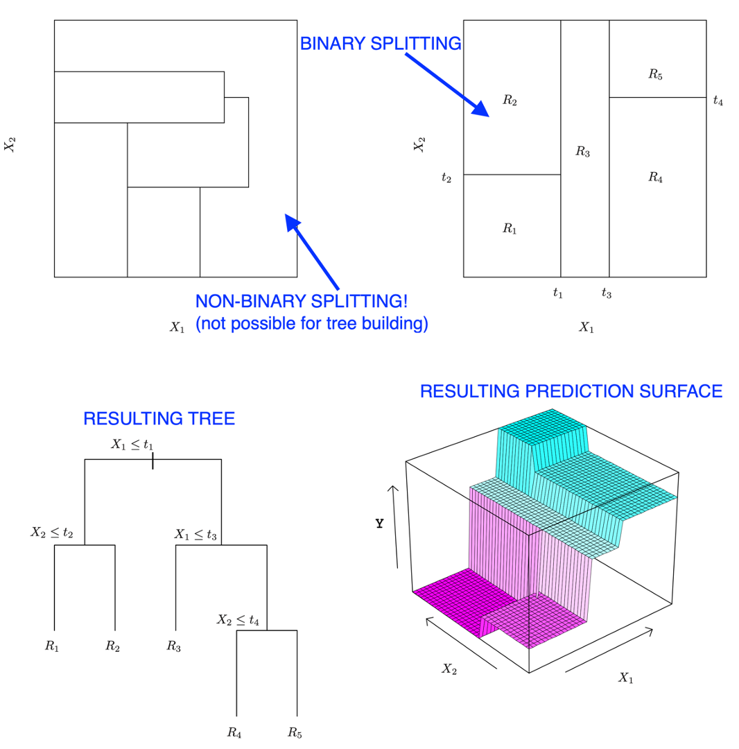
In this course, the algorithm will find these splitting points for you, but it is important to note how these splits occur. First, the splits have to be linear (e.g., straight). Second, they always have to be perpendicular to existing lines (e.g., no diagonal lines). Third, the split lines have to fully cross an existing box (e.g., no stopping halfway). These rules are demonstrated in the figure below, which shows a correct splitting and an incorrect splitting. It also further demonstrates the resulting decision tree and the associated plot. 

Introduction to Statistical Learning

Credit: Adapted from James et al. “Introduction to Statistical Learning.” Minor edits made by Renee Obringer. Source placeholder. date.  

Due to these rules about splitting, the decision tree model is ideal for nonlinear data. As demonstrated in the figure below, if there is a linear relationship (e.g., a straight diagonal line), then the tree-based model will not be able to accurately match the relationship. 

Introduction to Statistical Learning

Credit: Adapted from James et al. “Introduction to Statistical Learning.” Minor edits made by Renee Obringer. Source placeholder. date.

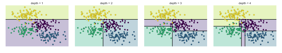
One of the disadvantages to decision trees is that they tend to overfit. That is, when the model is creating the boxes, it can get to the point where there is only one point in each box. This is a model that is “overfit” because if we try to make a prediction with new data, we won't be able to get an accurate prediction since the model is so specific to the exact data point in each box. This represents a challenge in a number of machine learning applications, where users have to balance an accurately trained model while avoiding overfitting the model. The figure below shows how the model is more likely to be overfit as we increase the depth of the tree. In other words, as the tree becomes more complex, it is also more likely to be overfit. Thus, for decision trees, the solution to overfitting is to build a lot of simple trees and aggregate them together into a “forest”, which we discuss in the next section.

Enter caption here

Jake VanderPlas. “In-Depth: Decision Trees and Random Forests”  excerpt from Python Data Science Handbook. Text is released under the CC-BY-NC-ND license, and code is released under the MIT license. 

 Assess It: Check Your Knowledge