1.2.3 Running a tool from its GUI

Let’s start by opening a tool from the Catalog pane and running it using its graphical user interface (GUI).

1. If, by chance, you still have the Buffer tool open from the previous section, close it for now so you can add some data.
2. Create a folder on your machine at C:\PSU\Geog485. If you use a different path, be sure to substitute your path in the following examples.
3. Download the Lesson 1 data and extract Lesson1.zip into your new folder so that the data is under the path C:\PSU\Geog485\Lesson1. This folder contains a variety of datasets you will use throughout the lesson.
4. Open a new project in Pro if you don't have one open already.  
5. Click the Add Data button  and browse to the data you just extracted. Add the us_boundaries and us_cities shapefiles.
6. Open the Geoprocessing pane if necessary and browse to the Buffer tool as you did in the previous section.
7. Double-click the Buffer tool to open it.

8. Examine the first required parameter: Input Features. Click the Browse button  and browse to the path of your cities dataset C:\PSU\Geog485\Lesson1\us_cities.shp. Notice that once you do this, a name is automatically supplied for the Output Feature Class (and the output path is the same as the input features). The software does this for your convenience only, and you can change the name/path if you want.

   A more convenient way to supply the Input Features is to just select the cities map layer from the dropdown menu. This dropdown automatically contains all the layers in your map. However, in this example, we browsed to the path of the data because it’s conceptually similar to how we’ll provide the paths in the command line and scripting environments.

9. Now you need to supply the Distance parameter for the buffer. For this run of the tool, set a Linear unit of 5 miles. When we run the tool from the other environments, we’ll make the buffer distance slightly larger, so we know that we got distinct outputs.
10. The rest of the parameters are optional. The Side Type parameter applies only to lines and polygons, so it is not even available for setting in the GUI environment when working with city points. However, change the Dissolve Type to Dissolve all output features into a single feature. This combines overlapping buffers into a single polygon.
11. Leave the Method set to Planar.  We're not going to take the earth's curvature into account for this simple example.
12. Click Run to execute the tool.
13. The tool should take just a few seconds to complete. Examine the output that appears on the map, and do a “sanity check” to make sure that buffers appear around the cities, and they appear to be about 5 miles in radius. You may need to zoom in to a single state in order to see the buffers.
14. Click on Pro's Analysis tab, then on History (in the Geoprocessing button group). This will open the History tab in Pro's Catalog pane, which lists messages about successes or failures of all recent tools that you've run.

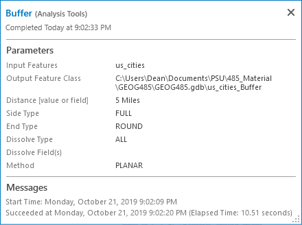
15. Hover over the Buffer tool entry in this list to see a pop-out window. This window lists the tool parameters, the time of completion, and any problems that occurred when running the tool (see Figure 1.1). These messages can be a big help later when you troubleshoot your Python scripts. The text of these messages is available whether you run the tool from the GUI, from the Python window in Pro, or from scripts.

Figure 1.1 Screen capture showing the Buffer tool and all messages.