EME 210
Data Analytics for Energy Systems

Confidence Intervals: The Standard Error Method

PrintPrint

  Read It: Confidence Intervals: The Standard Error Method

To determine the 95% confidence interval through the standard error method, we use the following equation

x + /   2 * S E

This equation centers the confidence interval around the sampling distribution mean (" x "), as shown in the figure below.

confidence interval around the sampling distribution mean
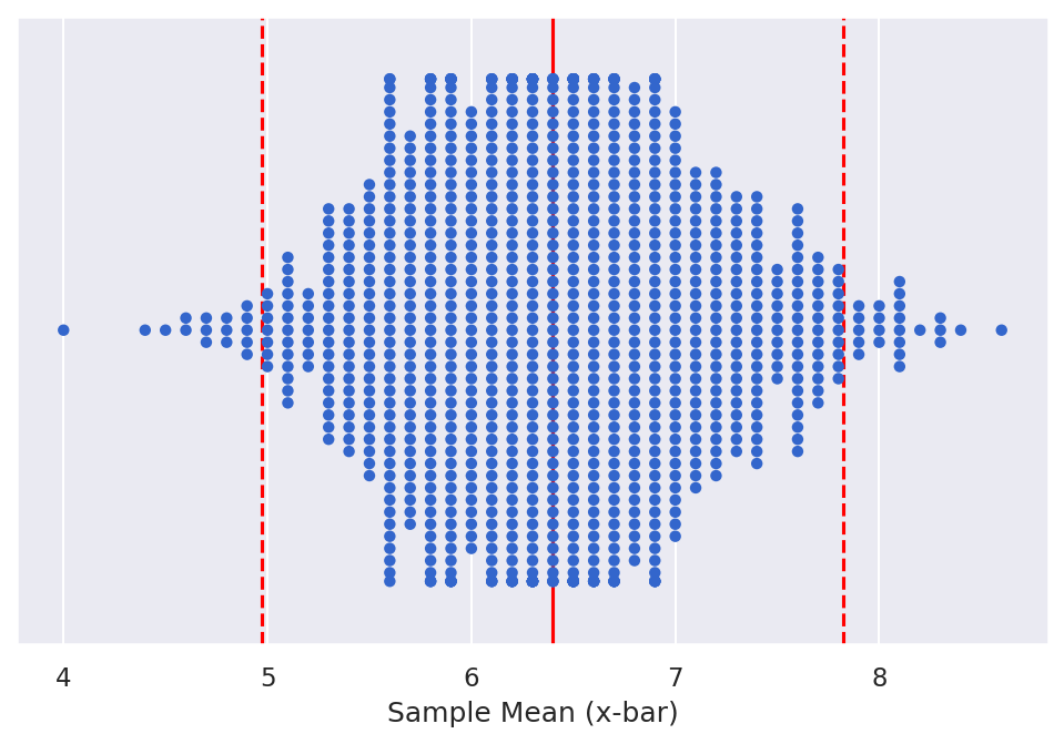
Confidence interval around the sampling distribution mean (" x  ―  ")
Credit: Eugene Morgan © Penn State is licensed under CC BY-NC-SA 4.0(link is external) 

In order to calculate this, we take three key steps in the code, following the development of the bootstrapped sampling distribution.

  1. Calculate the mean of the bootstrapped sampling distribution using  mean() 
  2. Calculate the standard error of the bootstrapped sampling distribution using  std() 
  3. Calculate the 95% confidence interval using the equation above

Below we demonstrate this process.

  Watch It: Video - Introduction to Sampling Distributions (07:12 minutes)

Click here for a transcript.

Welcome back to our series on bootstrapping. We left off the previous video after having made this plot where we show the bootstrapping distribution compared to the actual data in the original sample means. What we primarily use bootstrapping for is to do statistical inference. We want a larger sample size so that we can feel more confident in our final statistical inference. And one of those things is performing confidence intervals. And so a confidence interval is generally going to be two numbers. We've got the mean plus or minus something times the standard error. And so depending on the confidence level, you can have different calculations. We're going to focus on the 95 percent confidence interval. As this is by far the most common confidence level that you will see. In practice as well as in this course.

And so there are three steps to calculating the confidence interval with the bootstrap samples. The first is to actually calculate X bar. So what the average of the sample means is. and so it is critical to note that everything that we're doing with confidence intervals is on the bootstrapped sample distribution. So we're using boot means, which we calculated up here to show right here. And so essentially we want boot means bootstrap sample means dot mean. So the average of the sampling distribution. And so then we can print, x r is. So this is our mean that goes into these equations. The next step is to calculate the standard error. And recall from our previous video we are working with the standard error because we're working with a sampling distribution. So we say s e is root means, bootstrap sample means dot STD. Then we can also print that. We can say s e is.

And so now we have the standard error. And so now we're ready, that's the only two things we need in order to calculate the confidence interval with the bootstrap distribution. And so we can create an array using square brackets, where the first value is XB minus 2 times SE, and the second value is XB plus 2 times SE. And then we can print that, and we could just print you know CI similar to what we've been doing up here, but to show you a slightly different way to print things, still using the print button. Instead of just typing out the variable name here, I'm going to use a mini function. So I'm going to say round Y to the third decimal place for all Y in CI. And so, similar to our for loops, this Y is just a placeholder. It just needs to be this to match that, and then it'll figure out as the Y's apply to our values in CI. so if we run that we can see the 95 percent confidence interval is 5.058, 7.75.

And so that is all you need to do in order to get the confidence interval. But if we wanted to visualize it, I'm actually going to come up here and take this lot from our previous video, audit here for reference. We want to add the 95 confidence interval to this. So we have a new geom. This is called error bar H for horizontal AES. We give it a y value. And this is just going to be the position on the y-axis based off of what numbers we see here. So I'm just going to do 0.5 to put it halfway, and then we need to give it the X min of our error bar. So this is the first value of CI but attached to the zero width index. And then we do the same for x max. here CI 1 and outside the AES we can give it a color and say red. And then we're going to also add a point, a single point here. We're going to say same y. but our X is going to actually be X bar so that we sort of show where the sample, the mean of the sampling distribution is in reference to our confidence interval. Again, outside the AES we say color is red, and we'll give it a sufficiently large size so that it stands out. So if we run this we can see that now we've added this confidence interval to our lot, and we've got our X bar here in the middle which lines up with the middle of our normal distribution. And we can see here and so with our confidence interval, essentially we're saying that we're 95 percent confident that the true mean lies within this interval. So this is how you can add the confidence interval to the plot after calculating it.

Credit: © Penn State is licensed under CC BY-NC-SA 4.0

  Watch It: Video - Confidence Intervals SEmethod (04:58 minutes)

Click here for a transcript.

Welcome back to another video on confidence intervals and bootstrapping. Where we left off, we developed this plot to show our bootstrap or our confidence interval using the bootstrap sampling distribution. We're going to continue to build up that plot, but we're going to use the original samples. And so the process of calculating the confidence intervals is still the same.

I'm going to create XBD or X bar data, and we're going to use the data means, which if we scroll back up here beta means has our original four samples and those sample means. And so, we want the mean of those four samples, and I won't do any fancy printing here. Just show you what the thing is. I had a typo again with the capitalization. You have to make sure it's exact. But we can see this is what our data X bar is. similarly, we can calculate the standard error with data means.

And so here we can see. Oh, I forgot my parentheses there. And so we can see a single value here for our data standard error. And then we can calculate the confidence interval SID. So here we would say XBD minus 2 times SED. And then XBD plus 2 times SED. And so here we have our basic confidence interval for the data. And then we can build up this plot. So once again I'm going to copy this. I'm going to bring it down here and run it again to show you what we had before. And so now we want to add in the data confidence interval. So again we have this geom error bar H AES. We'll put this down a little lower. So we'll put it at 0.25. We still need to say x min is CID at the zero index and X max is CID at the one index. And then outside the AES we'll say color is, we'll make it green. And I'm going to add in an extra term called height, and this tells it how high we actually want V error bar to be. So it defaults to 0.5, so this is going from 0.25 to 0.75. I'll shorten this one so that it's 0.25. And then we also add the point at the middle. Making sure that our Y matches up so 0.25 and our X is at XBE. Our color is the same green, and we'll make it size three.

So if we run this, we can now see that we've got the confidence interval based off of the original four samples. It's much wider. That means that you know there was more variation, which is creating a wider confidence interval even though the means are fairly close to each other. So the benefit of doing that bootstrapping method is that because we have more samples, we're able to narrow our confidence interval a little bit, and therefore have a little bit more confidence in our statistical inference.

Credit: © Penn State is licensed under CC BY-NC-SA 4.0

  Try It: Apply Your Coding Skills in Google Colab

  1. Click the Google Colab file used in the video here.
  2. Go to the Colab file and click "File" then "Save a copy in Drive", this will create a new Colab file that you can edit in your own Google Drive account.
  3. Once you have it saved in your Drive, use the partial code below to calculate and plot the 95% confidence interval.

Note: You must be logged into your PSU Google Workspace in order to access the file. 

# step 1: calculate x bar
XB = ...

# step 2: calculate the standard error
SE = ...

# step 3: calculate the 95% Confidence Interval
CI = ...

(ggplot(boot_means) +
    geom_dotplot(...) +
    geom_vline(aes(xintercept = 7), color = 'blue', size = 1) +
    geom_errorbarh(...) +
    geom_point(...)
)


  Assess It: Check Your Knowledge

Knowledge Check

 FAQ

(add new questions)