EME 210
Data Analytics for Energy Systems

Summarizing Quantitative Data: Measures of Spread

PrintPrint

   Read It: Measures of Spread: Standard Deviation

In addition to knowing the center of a distribution of data values, it is often useful to know how dispersed or spread-out the distribution it. A common measure of this spread is the standard deviation:

Standard Deviation: the typical distance of a data value from the mean. s = ( x x ¯ ) 2 n 1

A larger standard deviation indicates a more dispersed collection of values, whereas a smaller standard deviation indicates a narrower distribution. To make the interpretation of the standard deviation more quantitative: a new, randomly drawn value from the population will have a 95% chance of being within the range -2 to +2 standard deviations from the mean (i.e., [ x 2 s ,   x + 2 s ] ). This is depicted in the example image below.
 

A histogram of a quantitative variable bell curve. 95% of the data is within two standard deviations from the mean.  Mean = 0.002 Media = 0.007 Standard Deviation = 0.997  At +2 standard deviation, the “z-score”: z*s = *s
Measures of Spread: Standard Deviation
Click for a text description of Measures of Spread: Standard Deviation.

A histogram of a quantitative variable. The vertical dark blue line is the mean, and the vertical red lines represent -2, -1, +1, and +2 standard deviations from the mean.

Credit: © Penn State is licensed under CC BY-NC-SA 4.0 

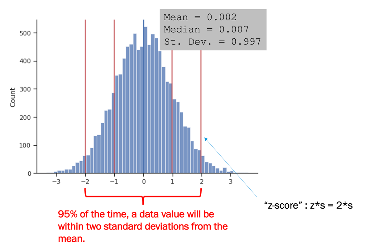
The image above also introduces the z-score, which we will come back to later in the course. The z-score, z , is simply the number (or fraction) of standard deviations that a value is from the mean. The z-score can be reported for a data point, or for a hypothetical value, such as the far right red line in the example above (where z = 2 ).

A Note on Notation

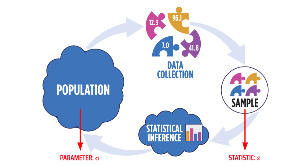
The formula above gives the standard deviation for a sample, noted s. The standard deviation for the entire population is noted with σ (or "sigma", a Greek letter). 

cyclical diagram showing how a data is collected from a population to quantify as a statistic to measure and make an inference; the standard deviation is noted and described in the text above
Notation for Standard Deviation
Click for a text description of Notation for Standard Deviation.
Enter Description Here

Credit: © Penn State is licensed under CC BY-NC-SA 4.0 

  Watch It: Video - Measures of Spread (4:36 minutes)

Click here for a transcript.

Hi, in this video we're going to keep on using the EPA flight data set. This is, these are facility level emissions of greenhouse gas data, but now to exemplify how to calculate measures of spread. So we're going to use those data to find standard deviation and then the interquartile range in Python. So, let's get to it. So first off, to find the standard deviation, we can find this in a very similar way as to how we found the mean and median above. So I'll do this in a print function, as we did before. So standard deviation is equal to, and then we call our whatever variable it is we want to do this on, 
so total reported direct emissions in this case. And our function now is not mean or median, but STD for standard deviation. And this actually shares the same units as the underlying variable. So in this case, millions of metric tons of CO2 equivalent. Okay, so our measure of spread, basically our measurement of how much these direct emissions vary across all the facilities in this data set, comes out to be a little bit more than a million. Pretty large number! Okay. Well, let's compare this to the interquartile range now. So we're going to calculate the interquartile range using the describe function. And there's different ways to do this describe function. I want to do it this way because the describe function is actually quite handy for a number of things. So let's first find that. So we'll call our variable total reported direct emissions, and our function here is just describe, and here we have to put in parentheses at the very end. And then we'll view the output.

Here we go. So this is a series actually, and it's got some, a lot of nice values. So we see our standard deviation here. We see our mean value. It also tells us how many values are being used here; so 6,481, in this case. Note the use of scientific notation here. And then the minimum zero, max of 20 million or so, and then 25, 50, and 75 percent. This 50 percent is the median. So this agrees with exactly what we had in the median above because this 50 percent 
refers to the 50th percentile. And that is another name for the median. So those are synonymous. And then we also have the 25th percentile, and the 75th percentile. So 25 percent of the values are less than 31,000 and some change, here. And 75 percent of the data values are less than 186,000 and some change here.

So our interquartile range is the difference between the 75th percentile and the 25th percentile. So we can simply find this by referencing these values in the describe series above. So it's our 75th percentile minus our 25th percentile. And you can view that value. Turns out to be 154 000 or so. So quite a bit less than standard deviation. So these are two different measures of the spread. The standard deviation is you know the typical distance away from the mean. And if you recall, in the comparison of the mean and median we have a right-skewed distribution up here. And so, our mean was a lot larger than our median. And so, there's a lot more spread about that mean, if we're looking about it that way. Whereas, the median and the interquartile range are much more concentrated down in this lower end where we have more observations.

So in summary, that's how you can find the standard deviation and the interquartile range. Along the way we found this handy describe function which is useful for summarizing the data in one fell swoop. And again, we got to do all this with the fascinating flight data set on greenhouse gas emissions across the U.S. Okay, thank you.

Credit: © Penn State is licensed under CC BY-NC-SA 4.0 

The above video demonstrates how to calculate standard deviation using the std function from Pandas. There is also a std function from Numpy, however in order to use that function to calculate standard deviation as given in the above formula, you need to specify the argument ddof=1 to represent the 1 being subtracted from n in the denominator:

numpy.std(x, ddof=1)

where x is an array of values.


  Try It: DataCamp - Find the standard deviation

You already found the mean and median of the total electricity consumed in a year (KHW) in the previous page.

HOME ID DIVISION KWH
10460 Pacific 3491.900
10787 East North Central 6195.942
11055 Mountain North 6976.000
14870 Pacific 10979.658
12200 Mountain South 19472.628
12228 South Atlantic 23645.160
10934 East South Central 19123.754
10731 Middle Atlantic 3982.231
13623 East North Central 9457.710
12524 Pacific 15199.859

* Data Source: Residential Energy Consumption Survey (RECS)(link is external), U.S. Energy Information Administration (accessed Nov. 15th, 2021)

Now can you find the standard deviation using Python?


  Assess It: Check Your Knowledge

Use the table below to answer the following questions.

Make Model Type City MPG
Audi A4 Sport 18
BMW X1 SUV 17
Chevy Tahoe SUV 10
Chevy Camaro Sport 13
Honda Odyssey Minivan 14


 FAQ