Click here for a transcript.
In this video, we're going to talk about some transformations and demonstrate how you can use these transformations to avoid breaking some of those linear conditions that we talked about earlier. So with that, let's go ahead and jump in.
So in this lesson we're going to use the RGGI data that we used during the Anova lesson. So, I've already got the data loaded and ready to go. So we can jump right in to linear regression. And so, as we start off most things, I want to start off with a plot. So I'm going to do df_merged, which is what I call that data frame, and then just do a point plot, so, x. We're going to do NOx_Base and compare it to NOx_RGGI. I forgot my y equals. And so, this is what the NOx_base in NOx_RGGI data set looks like. So it sort of follows this linear, but then there's all of these over here. And maybe we can classify those as outliers, but I think more likely that this is breaking our constant variance rule because this is a very obvious fan shape. Even though there's nothing really here, this is sort of the outline of a fan. And so, it probably is not the best linear model. We can go ahead and find out. We can say smf.ols, and we can do NOx_AGGI tilde NOx_base. Our data is the F merged. We need to specify has const equals true and I'm going to tack on the fit right onto the end. So then we can print results dot summary and see how the model is actually doing. So it's not terrible, r squared 0.748, that's surprisingly good given all of this out here. But nonetheless, this banding shape clearly breaks our constant variance rule.
And so, even though the linear regression is good, and in terms of the r squared technically it's not statistically valid. So, it would be better if we did a transformation, perhaps, in order to ensure that this that this linear model can be considered statistically valid. And so, what we are going to do is we're going to do a log transform in the hopes of remedying that increasing variability. And so, we can say merged log 10 NOx_base it's just NP dot log 10 BF merged NOx_base. And then I'm going to just repeat that but changing base to RGGI. And so, here we have this. We do get a warning that we encountered a divide by zero, but it didn't stop it from running. And so, we can just sort of move on. See if anything else causes an error, because it could have just created nan's that won't necessarily be bothersome. And so, if we go back and do our geom point plot, this time plotting log 10 and NOx_base and log 10 NOx_RGGI.
We can look at this, and we can say that the variance is no longer increasing, like there's no obvious fan shape. In fact, most of them are now clustered around an even stronger center line. These points out here, maybe now they can be considered outliers. We can't be sure though until we test it. But so far, it looks like our transformation did successfully reduce our variance. Now we just need to make sure we're not breaking another one of those rules, which is no outliers. So, in order to do that, we could do our IQR method and quickly calculate that. But I'm just going to do the visual method. So technically, the geombox plot that we use, it calculates outliers for us. And so, we can just say x equals zero. So this is the one where we need to sort of provide that weird x value, just needs to be any constant. So, x equals zero is common. And then y is log 10 NOx_base.
And so, in the base value there's no outliers. If there were, we would see these little stars up here, right? But we don't have any, so this is a good indication that there's at least no outliers in the base data. I'm going to come down here and paste that same code, change the suffix to RGGI. And there doesn't appear to be any outliers here as well, so in that case our newly transformed data is no longer breaking the increasing variability law, and it's not breaking the no outliers rule. So we are good to go, to do a regression. And so, I'm going to call this regression results 2. But we're still using the linear regression command OLS, but now we are regressing the RGGI log theta with the log theta of base. And again, data is merged df as const is equal to true. And then we can do the fit at the end. Then we can print results to dot summary, and run this... had the wrong order, df underscore merged.
And so, now we get this read, this error, and all it's telling us is that SVD did not converge. So we're having a lack of convergence, and the reason we keep this error in our demonstration is because it's a very strange error but it's very common with log transforms. You wouldn't know it from this SVD did not converge, but what is really being caused by this is the same thing that we got a warning about up here. We ended up with a zero in the log 10 data, which actually creates negative infinities for our data frame. It doesn't matter for the plotting, the plotting will just ignore those values. But it does matter for the actual regression.
So I'm going to leave this in here so that when you see this code you can recognize this error, and just be aware that if you do run into this that this is to go back up, make sure you check to see if you got that warning saying that you divided by zero. And then all you need to do is remove the negative infinities. And so, in order to do that, I'm just going to override the df_merged. And I'm going to say I want to keep df_merged, and just do two conditions, the first is where df_merged dot log 10 NOx underscore RGGI is not equal to negative np dot inf. So this is how we define infinity in Python, is np.inf, and specifically, we want to get rid of the negative versions and we want to get rid of those same values in our base code. So this is saying keep everything except where log 10 NOx_RGGI is, keep everything where this is not equal to negative infinity. And we're log 10 NOx_base is not equal to negative infinity, so we run that. I'm going to come up here, and grab the same regression line to avoid overwriting our previous results. I'm just going to change that to results three. And now we can see that it's running. And in fact, we've got these really high r squared values. So even though our linear regression, if we go up here, 0.748, not terrible. But now with this log transform we're up to close to 0.9, which is an incredible r squared. Our val, our model is now explaining 90 of the variance in the data. It's just important to remember that if we use any of these coefficients that they're on the log transform of the data and not on the original. So if we wanted to make a prediction, for example, we could do that. But if we wanted to apply it back to the original data we'd need to undo the log transform and just figure out what that real value is at that point.
 Read It: Transformations
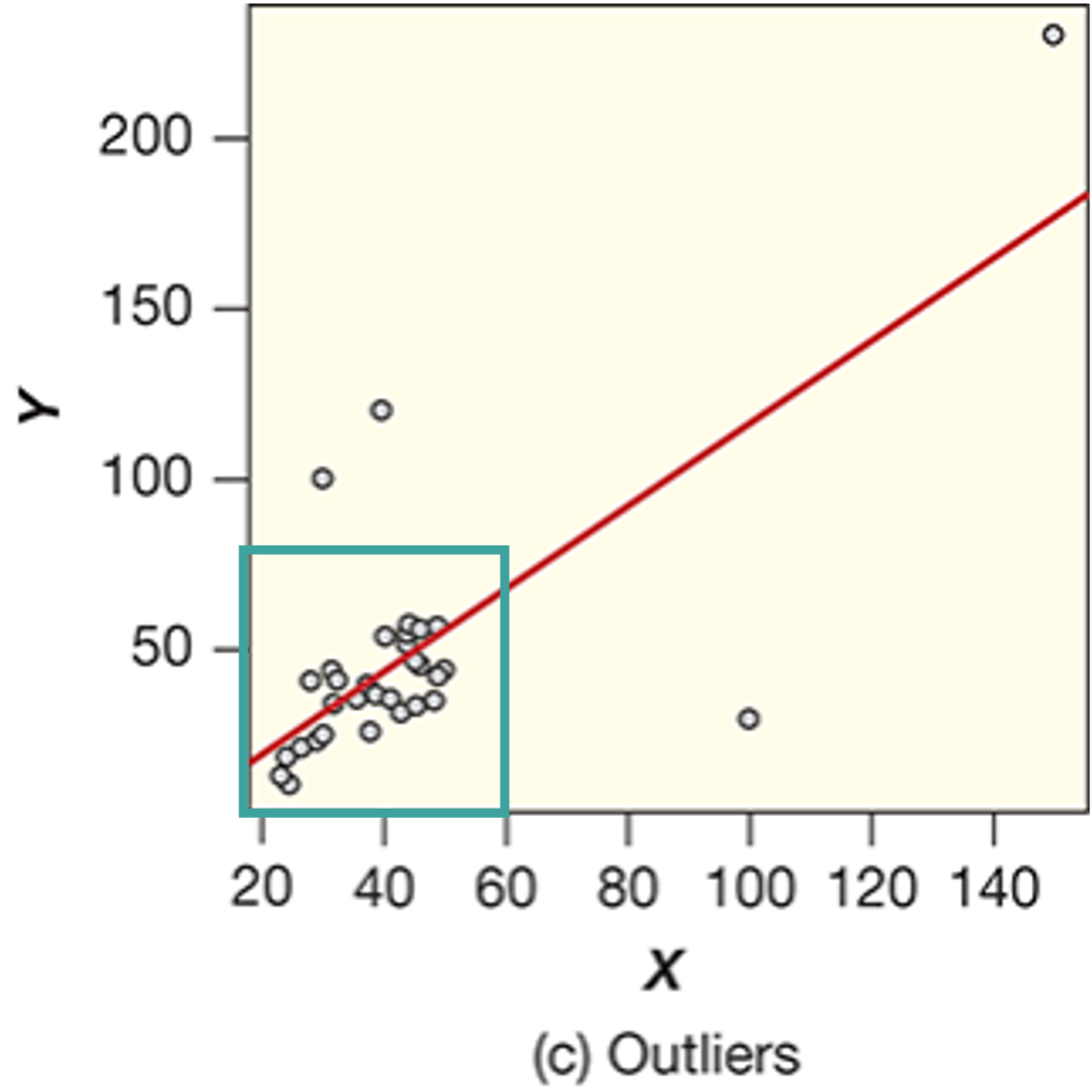
 Watch It: Video - Transformations (12:17 minutes)
 Try It: DataCamp - Apply Your Coding Skills
 Assess It: Check Your Knowledge