Introduction to Linear Regression

Introduction to Linear Regression

Read It: Introduction to Linear Regression

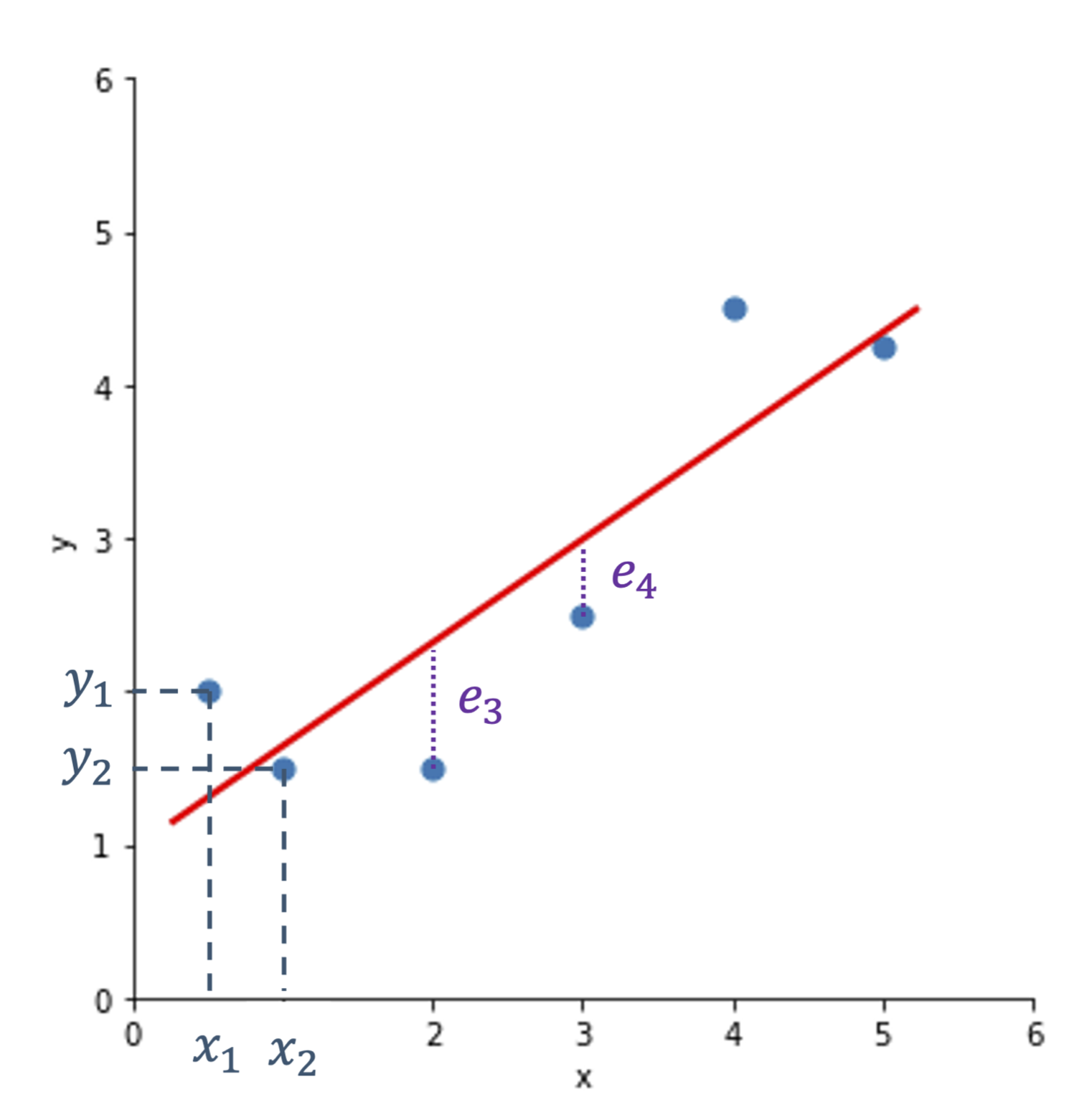
The goal of linear regression is to predict some value y based on the relationship between y and x. In practice, this means we try to find the best fit line to minimize the error. This is shown in the figure below, where we want to find the best line that minimizes the total difference between the data points and the line. The differences are denoted with the letter e. We then define the line based on the slope and intercept, ultimately following the classic equation: $y=mx+b$, where $\mathrm{m}$ is the slope and $b$ is the intercept.

Best Fit Line

Credit: © Penn State is licensed under CC BY-NC-SA 4.0

When working with a sample of data, we usually denote the line as: $y\mathrm{\_}i=b\mathrm{\_}1x\mathrm{\_}i+b\mathrm{\_}0+e\mathrm{\_}i$. For a population, we change the equation to include uppercase letters: $\mathrm{Y}=\text{ beta }1\mathrm{X}+\text{ beta }0\text{ + epsilon }$

A key aspect of this latter equation is that epsilon is normally distributed (e.g., $\mathrm{N}(0,\text{ sigma\_e })$). In fact, the normally distributed error is a critical assumption in linear regression models. Additional assumptions include: (a) a linear relationship between x and y, (b) constant variability in the data, and (c) no outliers present. Examples of how each of these conditions might be broken are provided below.

Figure A: 

Click for a text description.

$$\mathbf{A}=\left(\begin{array}{ccc}{a}_{11}& \cdots & a_{1n}\\ ⋮& \ddots & ⋮\\ a_{m1}& \cdots & a_{mn}\end{array}\right)$$

Credit: © Penn State is licensed under CC BY-NC-SA 4.0

Figure B: 

Click for a text description.

$$\mathbf{B}=\left(\begin{array}{ccc}{b}_{11}& \cdots & b_{1p}\\ ⋮& \ddots & ⋮\\ b_{n1}& \cdots & b_{np}\end{array}\right)$$

Credit: © Penn State is licensed under CC BY-NC-SA 4.0

Figure C: 

Click for a text description.

$$\mathbf{C}=\left(\begin{array}{ccc}{c}_{11}& \cdots & c_{1p}\\ ⋮& \ddots & ⋮\\ c_{m1}& \cdots & c_{mp}\end{array}\right)$$

Credit: © Penn State is licensed under CC BY-NC-SA 4.0

In particular, Figure (a) shows how the first condition (linearity) might be broken. Notice how the pattern is distinctly curved, rather than straight. In Figure (b), the second condition (constant variability) is broken. Here, we see a fan or wedge shape, which indicates that the variance between the y data at x = 20 is much larger than that at x = 10. This means that the variance is not constant, thus breaks one of the conditions for linear regression. Finally, Figure (c) shows the third condition (no outliers) being broken. In particular, there are four likely outliers, which leads to the broken condition. Below, is an example of an ideal example for meeting all three conditions. Notice that the pattern is relatively straight, without increasing variance, and there are no outliers. When conducting linear regression, this is how we want our data to look in an ideal world. Unfortunately, real-world data is rarely this perfect, so we often have to conduct transformations to ensure the model is statistically valid. We will go over these transformations later in the course.

 Assess It: Check Your Knowledge