Hypothesis Testing: Randomization Distributions
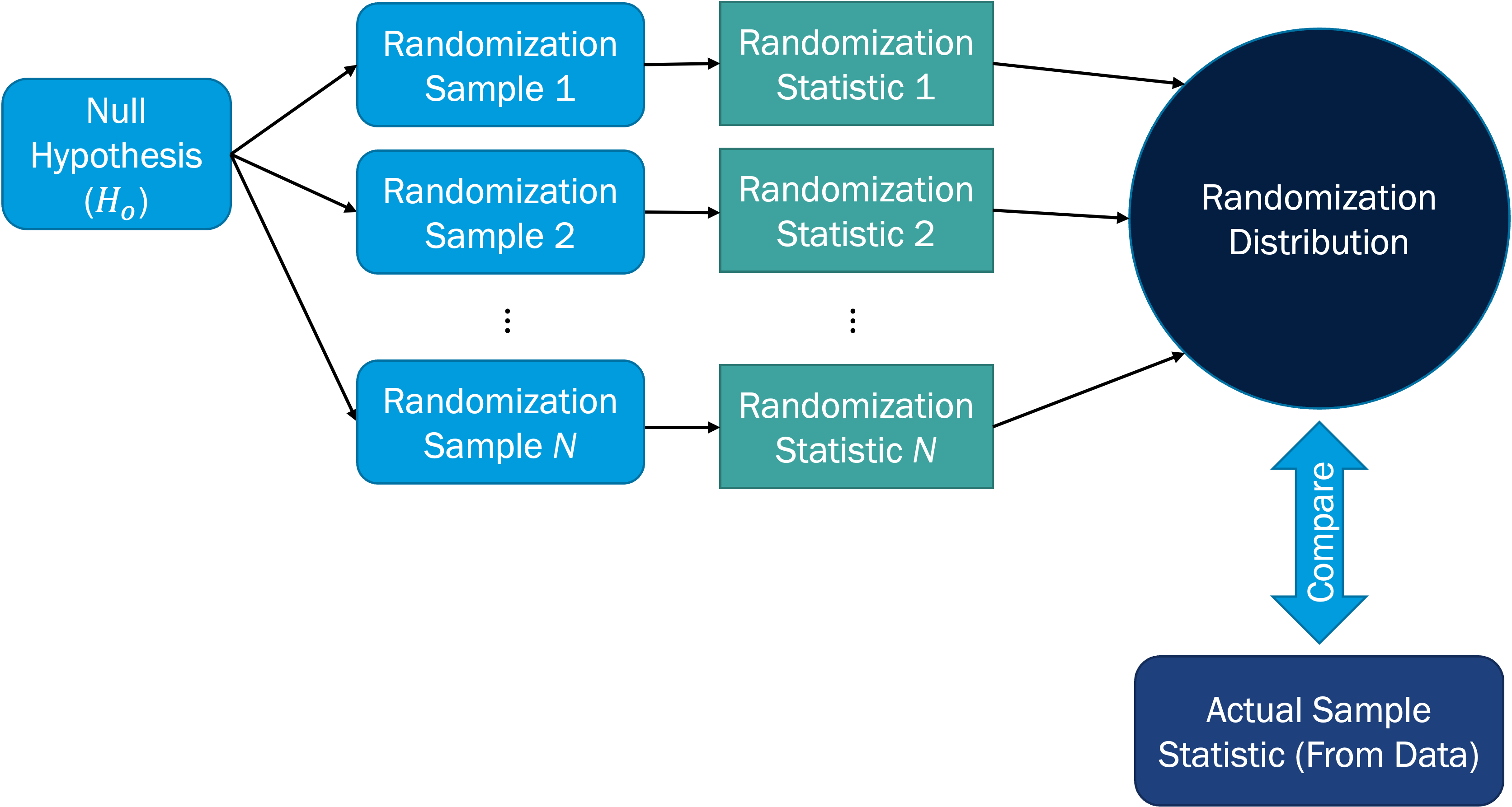
Like bootstrap distributions, randomization distributions tell us about the spread of possible sample statistics. However, while bootstrap distributions originate from the raw sample data, randomization distributions simulate what sort of sample statistics values we should see if the null hypothesis is true. This is key to using randomization distributions for hypothesis testing, where we can then compare our actual sample statistic (from the raw data) to the range of what we'd expect if the null hypothesis were to be true (i.e., the randomization distribution).
Randomization Procedure
The procedure for generating a randomization distribution, and subsequently comparing to the actual sample statistic for hypothesis testing, is depicted in the figure below.
The pseudo-code (general coding steps, not written in a specific coding language) for generating a randomization distribution is:
-
Obtain a sample of size n
-
For i in 1, 2, ..., N
-
Manipulate and randomize sample so that the null hypothesis condition is met. It is important that this new sample has the same size as the original sample (n).
-
Calculate the statistic of interest for the ith randomized sample
-
Store this value as the ith randomized statistic
-
-
Combine all N randomized statistics into the randomization distribution
Here, we've set the number of randomization samples to N = 1000, which is safe to use and which you can use as the default for this course. The validity of the randomization distribution depends on having a large enough number of samples, so it is not recommended to go below N = 1000. In the end, we have a vector or array of sample statistic values; that is our randomization distribution.
As we'll see in the subsequent pages, we'll use different strategies for simulating conditions under the assumption of the null hypothesis being true (Step 2.1 above). The choice of strategy will depend on the type of testing we're doing (e.g., single mean vs. single proportion vs. ...). Generally speaking, the goal of each strategy is to have the collection of sample statistics agree with the null hypothesis value on average, while maintaining the level of variability contained in the original sample data. This is really important, because our goal with hypothesis testing is to see what could occur just by random chance alone, given the null conditions are true, and then compare our data (representing what is actually happening in reality) to that range of possibilities.
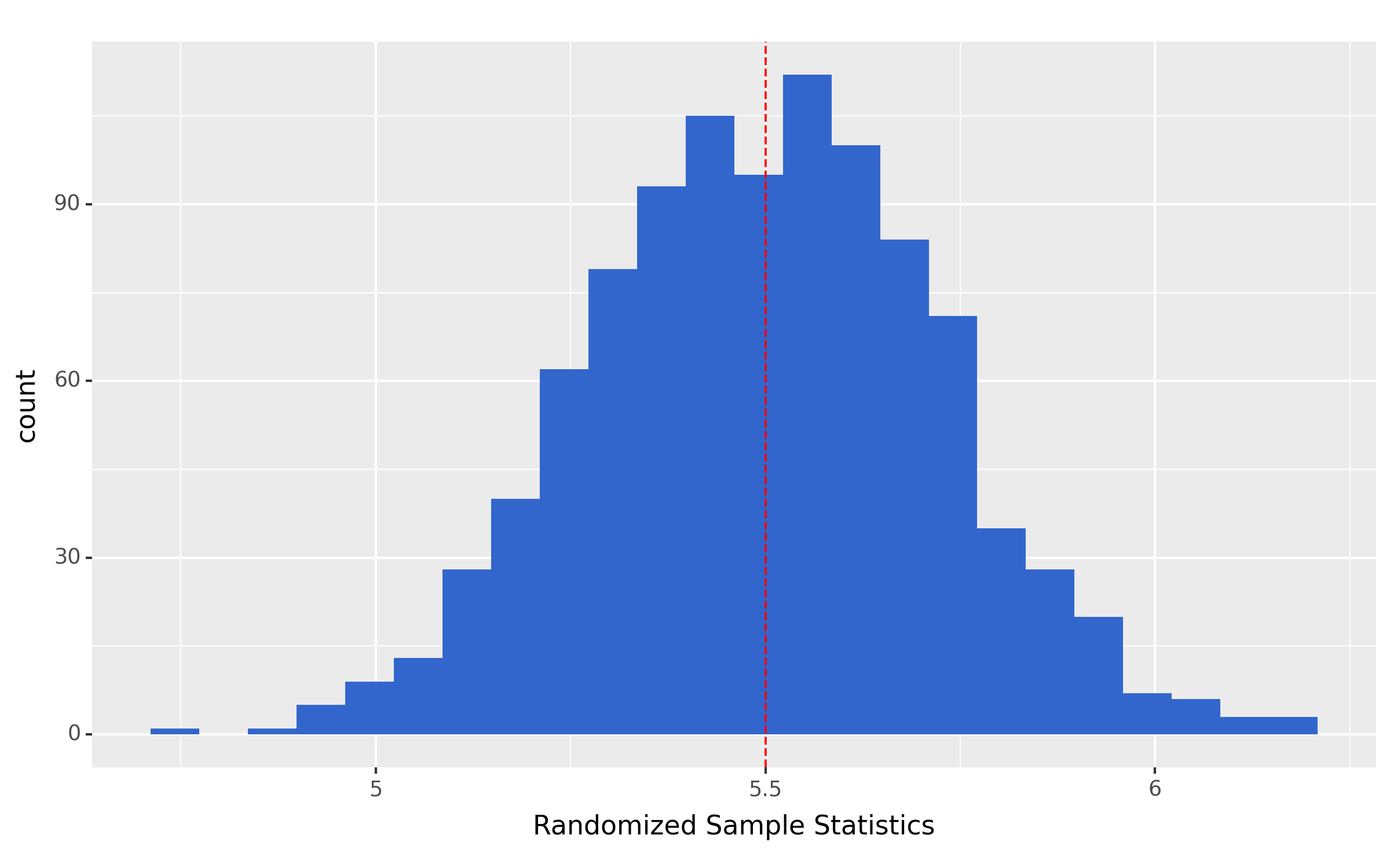
- The randomization distribution is centered on the value in the null hypothesis (the null value).
- The spread of the randomization distribution describes what sample statistic values would occur with random chance and given the null hypothesis is true.
The figure below exemplifies these key features, where the histogram represents the randomization distribution and the vertical red dashed line is on the null value.
The p-value
Our goal with the randomization distribution is to see how likely our actual sample statistic is to occur, given that the null hypothesis is true. This measure of likelihood is quantified by the p-value:
Let's elaborate on some important aspects of this definition and provide guidance on how to determine the p-value:
- The p-value is a probability, so it has a value between 0 and 1.
- This probability is measured as the proportion of samples in the randomization distribution that are at least as extreme as the observed sample (from the original data)
- "at least as extreme" refers to the inequality in the alternative hypothesis, and so:
- If the alternative is < (a.k.a. "left-tailed test"), the p-value = the proportion of samples the sample statistic.
- If the alternative is > (a.k.a. "right-tailed test"), the p-value = the proportion of samples the sample statistic.
- If the alternative is (a.k.a. "two-tailed test"), the p-value = twice the smaller of: the proportion of samples the sample statistic or the proportion of samples the sample statistic
The default threshold for rejecting or not rejecting the null hypothesis is 0.05, refer to as the "significance level" (more on this later). Thus,
- If the p-value < 0.05, we can reject the null hypothesis (in favor of the alternative hypothesis)
- If the p-value > 0.05, we fail to reject the null hypothesis
Although it should be noted that some researchers are moving away from the classical paradigm and starting to think of the p-value on more of a continuous scale, where smaller values are more indicative of rejecting the null.
 Assess It: Check Your Knowledge