Prioritize...
At the end of this section you should have a basic understanding of regression, know what we use it for, why we use it, and what the difference is between interpolation and extrapolation.
Read...
We began with hypothesis testing, which told us whether two variables were distinctly different from one another. We then used chi-square testing to determine whether one variable was dependent on another. Next, we examined the correlation, which told us the strength and sign of the linear relationship. So what’s the next step? Fitting an equation to the data and estimating the degree to which that equation can be used for prediction.
What is Regression?
Regression is a broad term that encompasses any statistical methods or techniques that model the relationship between two variables. At the core of a regression analysis is the process of fitting a model to the data. Through a regression analysis, we will use a set of methods to estimate the best equation that relates X to Y.
The end goal of regression is typically prediction. If you have an equation that describes how variable X relates to variable Y, you can use that equation to predict variable Y. This, however, does not imply causation. Likewise, similar to correlation, we can have cases in which a spurious relationship exists. But by understanding the theory behind the relationship (do we believe that these two variables should be related?) and through metrics that determine the strength of our best fit (to what degree does the equation successfully predict variable Y?), we can successfully use regression for prediction purposes.
I cannot stress enough that obtaining a best fit through a regression analysis does not imply causation and, many times, the results from a regression analysis can be misleading. Careful thought and consideration should be given when using the result of a regression analysis; use common sense. Is this relationship realistically expected?
Types of Regression
The most common and probably the easiest method of fitting, is the linear fit. Linear regression, as it is commonly called, attempts to fit a straight line to the data. As the name suggests, use this method if the data looks linear and the residuals (error estimates) of the model are normally distributed (more on this below). We want to again begin by plotting our data.
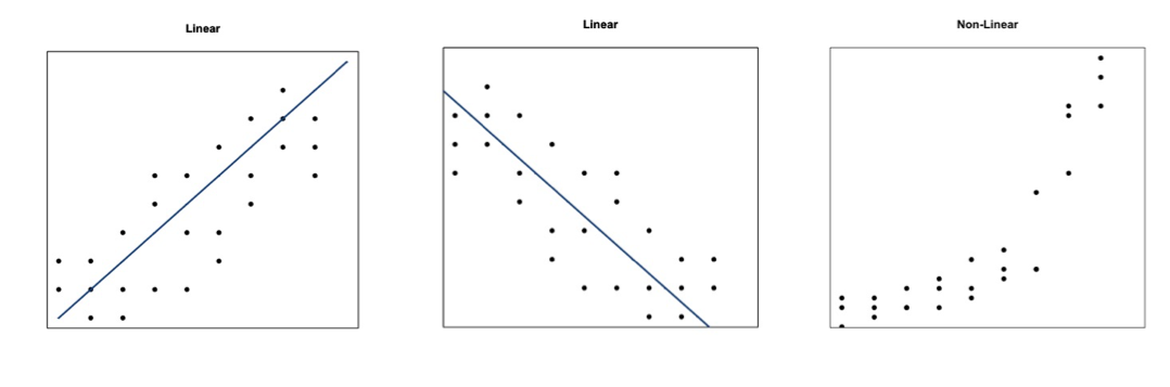
The figures above show you two examples of linear relationships in which linear regression would be suitable and one example of a nonlinear relationship in which linear regression would be ill-suited. So what do we do for non-linear relationships? We can fit other equations to these curves, such as quadratic, exponential, etc. These are generally lumped into a category called non-linear regression. We will discuss non-linear regression techniques along with multi-variable regression in the future. For now, let’s focus on linear regression.
Interpolation vs. Extrapolation
There are a number of reasons to fit a model to your data. One of the most common is the ability to predict Y based on an observed value of X. For example, we may believe there is a linear relationship between the temperature at Station A and the temperature at Station B. Let’s say we have 50 observations ranging from 0-25. When we fit the data, we are interpolating between the observations to create a smooth equation that allows us to insert any value from Station A, whether it has been previously observed or not, to estimate the value from Station B. We create a seamless transition between actual observations from variable X and values that have not occurred yet. This interpolation occurs, however, only over the range in which the inputs have been observed. If the model is fitted to data from 0-25, then the interpolation occurs between the values of 0 and 25.
Extrapolation occurs when you want to estimate the value of Y based on a value of X that’s outside the range in which the model was created. Using the same example, this would be for values less than 0 or greater than 25. We take the model and extend it to values outside of the observed data range.
Assuming that this pattern holds for data outside the observed range is a very large assumption. It could be that the variables outside this range follow a similar shape, such as linear, but the parameters of the equation could be entirely different. Alternatively, it could be that the variables outside of this range follow a completely different shape. It could be that the data follows a linear shape for one portion and an exponential fit for another, requiring two distinctly different equations. Although we won’t be focusing on predicting in this lesson, I want to make it clear the difference between interpolation and extrapolation, as we will indirectly employ this throughout the lesson. For now, I suggest only using a model from a regression analysis when the values are within the range of data it was created with (both for the independent variable, X, and dependent variable, Y).
Normality Assumption
When you perform a linear regression, the residuals (error estimates-this will be discussed in more detail later on) of the model must be normally distributed. This is more important later on for more advanced analyses. For now, I suggest creating a histogram of the residuals to visually test for normality or if your dataset is large enough you can use the central limit theory and assume normality.