Prioritize...
This section should prepare you for performing a regression analysis on any dataset and interpreting the results. You should understand how the squared error estimate is used, how the best fit is determined, and how we assess the fit.
Read...
We saw that the two point fit method is not ideal. It’s simplistic and can lead to large errors, especially if outliers are present. A linear regression analysis compares multiple fits to select an optimal one. Moreover, instead of simply looking at two points, the entire dataset will be used. One warning before we begin. It’s easy to use R and just plug in your data. But I challenge you to truly understand the process of a linear regression. What is R ‘doing’ when it creates the best fit? This section should answer that question for you, allowing you to get the most out of your datasets.
Squared Error
One way to make a fit estimate more realistic is to estimate the slope and offset multiple times and then take an average. This is essentially what a regression analysis does. However, instead of taking an average estimate of the slope and offset, a regression analysis chooses the fit that minimizes the squared error over all the data. Say, for example, we have 10 data points from which we calculate a slope and offset. Then, we can predict the 10 Y-values based on the observed 10 X-values and compute the difference between the predicted Y-values and the observed Y-values. This is our error; 10 errors in total. The closer the error is to 0, the better the fit.
Mathematically:
Where is the predicted value (the line), and Y is the observed value. Next, we square the error so that we don't have to worry about the sign of the error when we sum up the errors across our dataset. Here is the equation mathematically:
With the regression analysis, we are calculating the squared error for each data point based on a given slope and offset. For each fit estimate, we will provide a mean of the squared error. Mathematically,
For each observation, (i) we calculate the squared error and sum up all of the errors (N). Then divide by the number of errors estimated (N) to obtain the Mean Squared Error or MSE. The regression analysis seeks to minimize this mean squared error by making the best choice for a and b. While this could be done by trial and error, R has a more efficient algorithm which lets it compute these best values directly from our dataset.
Estimate Best Fit
In R, there are a number of functions to estimate the best fit. For now, I will focus on one function called ‘lm’. ‘lm’, which stands for linear models, fits your data with a linear model. You supply the function with your data, and it will go through a regression analysis (as stated above) and calculate the best fit. There is really only one parameter you need to be concerned about, and that is ‘formula’. The rest are optional, and it’s up to you whether you would like to learn more about them or not. The ‘formula’ parameter describes the equation. For our purposes, you will set the formula to y~x, the response~input.
There are a lot of outputs from this function, but let me talk about the most important and relevant ones. The primary output we will use will be the coefficients, which represent your model's slope and offset values. The next major output is the residuals. These are your error estimates (predicted Y – true Y). You can use these to calculate the MSE by squaring the residuals and averaging over them. If you would like to know more about the function, including the other inputs and outputs, follow this link on "Fitting Linear Models."
Let me work through an example to show you what ‘lm’ is doing. We are going to calculate a fit 3 times ‘by hand’ and choose the best fit by minimizing the MSE. Then we will supply the data to R and use the 'lm' function. We should get similar answers.
Let’s examine the temperature again from Tokyo, looking at the mean temperature supplied and our estimation of the average of the maximum and minimum values. After quality control, here is a list of the temperature values for 6 different observations. I chose the same 6 observations that I used to calculate the slope 3 different times from the previous example.
| Index | Average Temperature | (Max + Min)/2 |
|---|---|---|
| 1146 7049 |
37.94 57.02 |
39.0 54.5 |
| 18269 9453 |
39.02 50.18 |
38.0 46.5 |
| 6867 15221 |
62.78 88.34 |
62.5 88 |
Since I already calculated the slope and offset, I’m going to supply them in this table.
| Index | Slope | Offset |
|---|---|---|
| 1146 7049 |
0.8123690 | 8.1787210 |
| 18269 9453 |
0.7616487 | 8.2804660 |
| 6867 15221 |
0.9976525 | -0.1326291 |
We saw that the last fit estimate visually was the best, but let’s check it by calculating the MSE for each fit. Remember the equation (model) for our line is:
For each slope, I will input the observed mean daily temperature to predict the average of the maximum and minimum temperature. I will then calculate the MSE for each fit. Here is what we get:
| Index | MSE |
|---|---|
| 1146 7049 |
21.11071 |
| 18269 9453 |
54.16036 |
| 6867 15221 |
3.02698 |
If we minimize the MSE, our best fit would be the third slope and offset (0.9976525 and -0.1326291); confirming our visual inspection.
Let’s see how the ‘lm’ model in R compares. Remember, the model is more robust and will definitely give a different answer, but we should be in the same ballpark. The result is a slope of 1.00162 and an offset of -0.06058 with an MSE of 2.925. Our estimate was actually pretty close, but you can see that we’ve reduced the MSE even more by doing a regression analysis and have changed the slope and offset values slightly
Methods to Assess Goodness of Fit
Now that we have our best fit, how good is that fit? There are two main metrics for quantifying the best fit. The first is looking at the MSE. I told you that the MSE is used as a metric for the regression to pick the best fit. But it can be used in your end result as well. Let’s look at what the units are for the MSE:
The units for MSE will be the units of your Y variable squared, so for our example it would be (degrees Fahrenheit)2. This is kind of difficult to utilize. Instead, we will state the Root-Mean-Square-Error (RMSE) (sometimes called root-mean-square deviation RMSD). The RMSE is the square root of the MSE which will give you units that you can actually interpret, which in our example would be degrees Fahrenheit. You can think of the RMSE as an estimate of the sample deviation of the differences between the predicted values and the observed.
For our example, the MSE was 2.926 so the RMSE would be 1.71oF. The model has an uncertainty of ±1.71oF. This is the standard deviation estimate. Remember the trick we learned for normal distributions? 1 standard deviation is 66.7% of the data, 2 will be 95% and 3 will be 99%. If we multiply the RMSE by 2, you can attach the confidence level of 95%. That is, you are 95% certain that the predicted values should lie within this range of ±2 RMSE.
The second metric to calculate is the coefficient of determination, also called R2 (R-Squared). R2 is used to describe the proportion of the variance in the dependent variable (Y) that is predicted from the independent variable (X). It really describes how well variable X can be used to predict variable Y and capture not only the mean but the variability. R2 will always be positive and between 0 and 1-the closer to 1 the better.
In our example with the Tokyo temperatures, the R2 value is 0.9859. This means that the mean temperature explains 98.5% of the variability of the average max/min temperature.
Let’s end by plotting our results to visually inspect whether the equation selected through the regression is good or not. Here is our data again, with the best fit determined from our regression analysis in R. I’ve also included dashed lines that represent our RMSE boundaries (2*RMSE=95% confidence level).
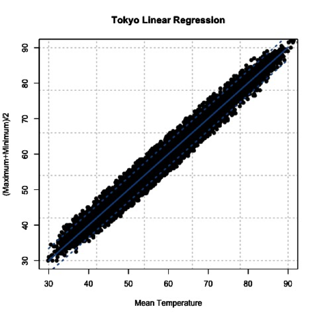
By using the slope and offset from the regression, the line represents the values we would predict. The dashed lines represent our uncertainty or possible range of values at the 95% confidence level. Depending on the confidence level you choose (1, 2, or 3 RMSE), your dashed lines will either be closer to the best fit line (1 standard deviation) or encompass more of the data (3 standard deviations).