Prioritize...
By the end of this section, you should be able to perform a regression tree analysis on a dataset and be able to optimize the model.
Read...
Sometimes we can overfit our model with too many parameters for the number of training cases we have. An alternative approach to multiple linear regression is to create regression trees. Regression trees are sort of like diagrams of thresholds. Was this observation above or below the threshold? If above, move to this branch; if below, move to the other branch. It's kind of like a roadmap for playing the game "20 questions" with your data to get a numerical answer.
Initial Analysis
Similar to the multiple linear regression analysis, we need to start with an initial tree. To create a regression tree for each response variable, we will use the function 'rpart'. When using this function, there are three ways a tree could stop growing.
- The complexity parameter, which describes the amount by which splitting that node improved the relative error (deviance), goes below a certain threshold (parameter cp).
- If the new branch does not improve by more than 0.01, the new branch is deemed nonessential.
- By default, cp is set to 0.01. This means that a new branch must result in an improvement greater than 0.01.
- The number of samples in the node is less than another threshold (parameter minsplit).
- You can set a threshold of the number of samples required in each node/breakpoint.
- By default, the minsplit is 20. This means that after each threshold break, you need to have at least 20 points to consider another break.
- The tree depth, the number of splits, exceeds a threshold (parameter maxdepth).
- You don't want really large trees. Too many splits will not be computationally efficient for prediction.
- By default, the max depth is set to 30.
Use the code below to create a regression tree for each variable. Note the indexing to make sure we create a tree with respect to other variables in the data set. I included one example (AcreageHarvested) of the summary results of the regression model.
The result is an initial threshold model for the data to follow. Use the code below to visualize the tree:
Your script should look something like this:
# plot regression trees
prettyTree(rt1.YieldAcre)
prettyTree(rt1.Production)
prettyTree(rt1.SeasonAveragePrice)
prettyTree(rt1.ValueofProduction)
prettyTree(rt1.AcreageHarvested)
The boxes represent end points (cutely called the leaves of the tree). The circles represent a split. The tree depth is 5 and the 'n' in each split represents the number of samples. You can see that the 'n' in the final boxes is less than 20, less than the minimum requirement for another split. Here is the tree for the response variable yield/acre.
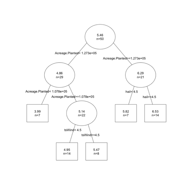
You can think of the tree as a conditional plot. In this example, the first threshold is acreage planted. If acreage planted is greater than 12,730 we then consider hail events. If hail is greater than 4.5 we expect a yield of 6.53 per acre.
Regression trees are easy in that you just follow the map. However, one thing you might notice is that your predictions are set values, and in this case there are 5 possible predictions. You don't capture variability as well relative to linear models.
Pruning
Similar to the multiple linear regression analysis, we want to optimize our model. We want a final tree that minimizes the error of the predictions but also minimizes the size of the tree which tend to generalize poorly for forecasting by fitting the noise in the training data. We do this by 'pruning', deciding which splits provide little value and removing them. Again, there are a variety of metrics that can be used for optimizing.
One option would be to look at the number of samples (n= value in each leaf). If you have a leaf with a small sample size (<5,10 - it depends on the number of samples you actually have), you might decide that there aren't enough values to really confirm whether that split is optimal. Another option is to obtain the subtrees and calculate the error you get for each subtree. Let’s try this out; run the code below to use the command 'printcp'.
What is displayed here? Our whole tree has 4 ‘subtrees’, so the results are broken into 5 parts representing each subtree and the whole tree. For each subtree (and the whole tree), we have several values we can look at. The first relevant variable is the relative error (rel error). This is the error compared to the root node (the starting point of your tree) and is calculated using a ten-fold cross-validation process. This process estimates the error multiple times by breaking the data into chunks. One chunk is the training data, which is used to create the model, and the second chunk is the test data, which is used to predict the values and calculate the error. For each iteration, it breaks the data up into new chunks. For 10-fold cross validation, the testing chunk always contains 1/10 of the cases and the training chunk 9/10. This lets R calculate the error on independent data in just 10 passes while still using almost all of the data to train each time. You can visualize this process below.
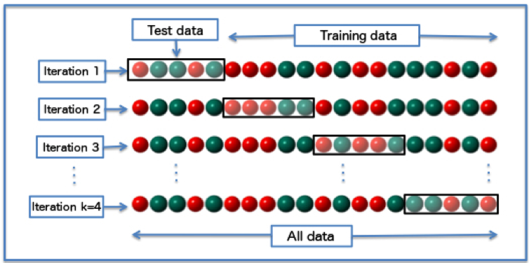
#/media/File:K-fold_cross_validation_EN.jpg)
For more information on cross-validation, you can read the cross-validation wiki page. The xerror is an estimate of the average error from the 10 iterations performed in the cross- validation process.
Let’s look at the results from our yield/acre tree.
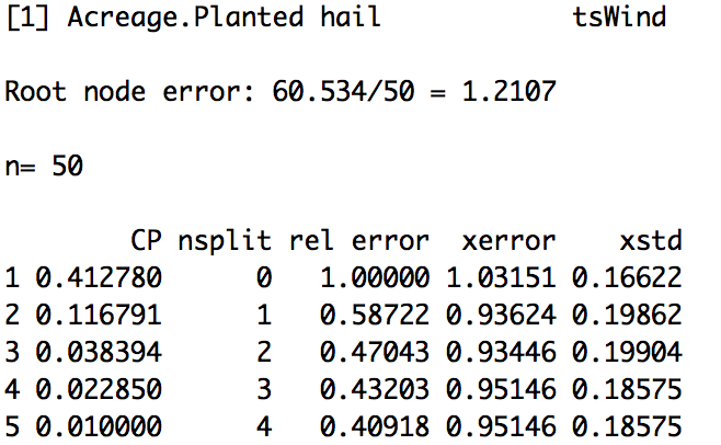
(Please note that your actual values may be different because the cross-validation process is randomized). The average error (xerror) is lowest at node 3 or split 2. You would prune your tree at split 2 (remove everything after the second split).
An alternative and more common optimization method is the One Standard Error (1 SE) rule. The 1 SE rule uses the xerror and xstd (average standard error). We first pick the subtree with the smallest xerror. In this case, that is the third one (3). We then calculate the 1 SE rule:
xerror+1*xstd
In this case, it would be 0.93446+0.19904=1.1325. We compare this value to the relative error column (rel error). The rel error represents the fraction of wrong predictions in each split compared to the number of wrong predictions in the root. For this example, the first split results in a rel error of 0.587, meaning the error in this node is 58% of that in the first node (we have improved the error by 1-0.587 or 41%). However, the rel_error is computed using the training data and thus decreases as the tree grows and adjusts to the data. We should not use this as an estimate of the real error, instead we minimize the xerror and xstd which uses the testing data. We still want to minimize the rel_error, so we select the first split that has a rel_error less than 1.1325 (the 1 SE rule). In this case, that is tree 1. To read how xerror, rel_error, and xstd are calculated in this function, please see the documentation.
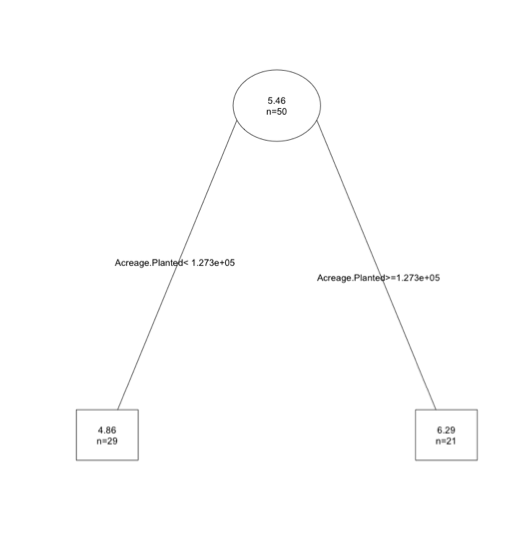
If we want to prune our tree using this metric, we would prune the tree to subtree 1. To do this in R, we will use the 'prune' function and insert the corresponding cp value to that tree, in this case 0.4. Run the code below to test this on the YieldAcre variable.
You will end up with the first tree- visually:
This may seem a bit confusing, especially the metric portion. All you should know is that if using the 1 SE rule, we calculate a threshold (xerror+1*xstd) and find the first node with a relative error less than this value. Remember, the key here is we don't want the most extensive tree; we want one that predicts relatively well but doesn't over fit.
Automate
The good thing is that we can automate this process. So if you don't understand the SE metric well, don't fret. Just know that it's one way of optimizing the error and length of the tree. To automate, we will use the function rpartXse.
Your script should look something like this:
# automate process
(rtFinal.YieldAcre <- rpartXse(Yield.Acre~.,lapply(stateData[,c(4,6,10:12)],as.numeric)))
(rtFinal.Production <- rpartXse(Production~.,lapply(stateData[,c(4,7,10:12)],as.numeric)))
(rtFinal.SeasonAveragePrice <- rpartXse(Season.Average.Price~.,lapply(stateData[,c(4,8,10:12)],as.numeric))) (rtFinal.ValueofProduction <- rpartXse(Value.of.Production~.,lapply(stateData[,c(4,9:12)],as.numeric)))
(rtFinal.AcreageHarvested <- rpartXse(Acreage.Harvested~.,lapply(stateData[,c(4:5,10:12)],as.numeric)))
Again, you need to remember that due to the ten-fold cross validation, the error estimates will be different if you rerun your code.