Prioritize...
After reading this section you should be able to obtain the best model and use it.
Read...
Now we know which model is best (linear, regression forest, or random forest). But how do we actually obtain the model parameters and use it?
Obtain Model
At this point, we have determined which type of model best represents the response variable but we have yet to actually obtain the model in a usable way. Let's extract out the best model for each response variable. Start by determining the best model names.
# obtain the best model for each predicted variable
NamesBestModels <- sapply(bestScores(allResults),
                          function(x) x['nmse','system'])
Next, classify the model type.
modelTypes <- c(cvRF='randomForest',cvRT='rpartXse',cvLM='lm')
Now create a function to apply each model type.
modelFuncs <- modelTypes[sapply(strsplit(NamesBestModels,split="\\."),
                         function(x) x[1])]
Then obtain the parameters for each model.
modelParSet <- lapply(NamesBestModels,
                   function(x) getVariant(x,allResults)@pars)
Now we can loop through each response variable and save the best model.
Your script should look something like this:
bestModels <- list()
for(i in 1:length(NamesBestModels)){
  form <-as.formula(paste(names(clean.stateData)[4+i],'~.'))
  bestModels[[i]]<- do.call(modelFuncs[i],
                            c(list(form,lapply(clean.stateData[,c(4,4+i,10:12)],as.numeric)),modelParSet[[i]]))
}
The code above begins by creating a formula for the model (response variable~factor variable). It then calls the 'modelFuncs' function, which is our learners (lm, randomForest, rpartXse), and supplies the arguments and the parameters. You are left with a list of five models. For each response variable, the list contains the formula of the best model.
Predict
Now that we have the formulas, let's try predicting values that were not used in the training set. Here is a set of corn and storm data from 2010-2015. We can use this data to test how well the model actually does at predicting values not used in the training dataset. Remember, the reason I didn't use this dataset for testing before was due to the limited sample size but we can use it as a secondary check.
Begin by loading the data and extracting it out for our state of interest (Minnesota).
Your script should look something like this:
# load in test data
mydata2 <- read.csv("finalProcessedSweetCorn_TestData.csv",stringsAsFactors = FALSE)

# create a data frame for this state
stateData2 <- subset(mydata2,mydata2$State == state)
Now we will predict the values using the best model we extracted previously.
Your script should look something like this:
# create predictions
modelPreds <- matrix(ncol=length(NamesBestModels),nrow=length(stateData2$Observation.Number))
for(i in 1:nrow(stateData2))
  modelPreds[i,] <- sapply(1:length(NamesBestModels),
                           function(x)
                             predict(bestModels[[x]],lapply(stateData2[i,4:12],as.numeric))
  )
modelPreds[which(modelPreds < 0)] <-0
We loop through each observation and apply the best model for each response variable. We then replace any non-plausible predictions with 0. You are left with a set of predictions for each year for each corn response variable. Although we have only 6 years to work with, we can still calculate the NMSE to see how well the model did with data not included in the training dataset. The hope is that the NMSE is similar to the NMSE calculated in our process for selecting the best model.
Your script should look something like this:
# calculate NMSE for all models
avgValue <- apply(data.matrix(clean.stateData[,5:9]),2,mean,na.rm=TRUE)
apply(((data.matrix(stateData2[,5:9])-modelPreds)^2),
        2,mean,na.rm=TRUE)/
        apply((scale(data.matrix(stateData2[,5:9]),avgValue,F)^2),2,mean)
The code starts by calculating an average value of each corn response variable based on the longer dataset. Then we calculate the MSE from our 6-year prediction and normalize it by scaling the test data by the long-term average value. You should get these scores:
| Average.Harvested | Yield.Acre | Production | Season.Average.Price | Value.of.Production |
|---|---|---|---|---|
| 0.1395567 | 0.7344319 | 0.4688927 | 0.6716387 | 0.7186660 |
For comparison, these were the best scores during model selection. Remember, the ones listed below may be different from yours due to the random factor in the k-fold cross-validation.
$Acreage.Harvested
       system     score
nmse cv.lm.v1 0.2218191

$Yield.Acre
       system    score
nmse cv.rf.v2 0.624105

$Production
       system     score
nmse cv.lm.v1 0.2736667

$Season.Average.Price
       system     score
nmse cv.rf.v3 0.4404177

$Value.of.Production
       system     score
nmse cv.lm.v1 0.4834414
The scores are relatively similar. Yield/acre has the highest score while the lowest score is from acreage harvested and production. This confirms that our factor variables are better at predicting the acreage harvested than Yield/Acre.
US Example
Let’s go through one more example of the whole process for the entire United States (not just Minnesota). In addition, I'm going to use more factor variables and only look at observations after 1996 (this will include events such as flash floods, wildfires, etc.).
To start, let's extract out the data from 1996 onward for all states.
Your script should look something like this:
# extract data from 1996 onward to get all variables to include
allData <- subset(mydata,mydata$Year>= 1996)
Now clean up the data. I've decided that if no events happen, I will remove that event type. Start by summing up the number of events for each event type (over the whole time period) and determining which factor variables to keep.
Your script should look something like this:
# compute total events
totalEvents <- apply(data.matrix(allData[,4:34]),2,sum,na.rm=TRUE)
varName <- names(which(totalEvents>0))
Now subset the data for only event types where events actually occurred and remove any missing cases.
Your script should look something like this:
# subset data for only events where actual events occurred
clean.data <- allData[varName]
clean.data <- clean.data[complete.cases(clean.data),]
Now create the functions to train, test, and evaluate the different model types.
Your script should look something like this:
# create function to train test and evaluate models through cross-validation
cvRT <- function(form,train,test,...){
     modelRT<-rpartXse(form,train,...)
     predRT <- predict(modelRT,test)
     predRT <- ifelse(predRT <0,0,predRT)
     mse <- mean((predRT-resp(form,test))^2)
     c(nmse=mse/mean((mean(resp(form,train))-resp(form,test))^2))
}
cvLM <- function(form,train,test,...){
     modelLM <- lm(form,train,...)
     predLM <- predict(modelLM,test)
     predLM <- ifelse(predLM <0,0,predLM)
     mse <- mean((predLM-resp(form,test))^2)
     c(nmse=mse/mean((mean(resp(form,train))-resp(form,test))^2))
}
library(randomForest)
cvRF <- function(form,train,test,...){
     modelRF <- randomForest(form,train,...)
     predRF <- predict(modelRF,test)
     predRF <- ifelse(predRF <0,0,predRF)
     mse <- mean((predRF-resp(form,test))^2)
     c(nmse=mse/mean((mean(resp(form,train))-resp(form,test))^2))
}
Now apply these functions to all the response variables.
Your script should look something like this:
# apply function for all variables to predict
dataForm <- sapply(names(clean.data)[c(2:6)],
                   function(x,names.attrs){
                     f <- as.formula(paste(x,"~."))
                     dataset(f,lapply(clean.data[,c(names.attrs,x)],as.numeric),x)
                   },
                   names(clean.data)[c(1,7:27)])
allResults <- experimentalComparison(dataForm,
                                     c(variants('cvLM'),
                                       variants('cvRT',se=c(0,0.5,1)),
                                       variants('cvRF',ntree=c(70,90,120))),
                                     cvSettings(5,10,100))
Finally, look at the scores.
Your script should look something like this:
# look at scores
bestScores(allResults)
Hopefully, by including more data points (in the form of multiple states) as well as more factor variables, we can decrease the NMSE. The best score is still for acreage harvested, with an NMSE of 0.0019, but production and value of production are quite good with NMSEs of 0.039 and 0.11 respectively.
Again the end goal is prediction, so let's obtain the best model for each response variable.
Your script should look something like this:
# obtain the best model for each predicted variable
NamesBestModels <- sapply(bestScores(allResults),
                          function(x) x['nmse','system'])
modelTypes <- c(cvRF='randomForest',cvRT='rpartXse',cvLM='lm')
modelFuncs <- modelTypes[sapply(strsplit(NamesBestModels,split="\\."),
                                function(x) x[1])]
modelParSet <- lapply(NamesBestModels,
                      function(x) getVariant(x,allResults)@pars)
bestModels <- list()
for(i in 1:length(NamesBestModels)){
   form <-as.formula(paste(names(clean.data)[1+i],'~.'))
  bestModels[[i]]<- do.call(modelFuncs[i],
                            c(list(form,lapply(clean.data[,c(1,i+1,7:27)],as.numeric)),
                              modelParSet[[i]])) }
And let's test the model again using the separate test dataset. We need to create a clean test dataset first.
Your script should look something like this:
# create a data frame for test data
data2 <- subset(mydata2,mydata2$Year >= 2010)

# subset data for only events where actual events occurred
clean.test.data <- data2[varName]
clean.test.data <- subset(clean.test.data,!is.na(as.numeric(clean.test.data$Acreage.Planted)))
Now calculate the predictions.
Your script should look something like this:
# create predictions
modelPreds <- matrix(ncol=length(NamesBestModels),nrow=nrow(clean.test.data))
for(i in 1:nrow(clean.test.data)){
  modelPreds[i,] <- sapply(1:length(NamesBestModels),
                          function(x)
                            predict(bestModels[[x]],lapply(clean.test.data[i,c(1,7:27)],as.numeric)))
}
modelPreds[which(modelPreds < 0)] <-0
Finally, calculate the NMSE.
Your script should look something like this:
# calculate NMSE for all models
avgValue <- apply(data.matrix(clean.data[,2:6]),2,mean,na.rm=TRUE)
apply(((data.matrix(clean.test.data[,2:6])-modelPreds)^2),
        2,mean,na.rm=TRUE)/
  apply((scale(data.matrix(clean.test.data[,2:6]),avgValue,F)^2),2,mean)
In this case, I get relatively high scores for every corn response variable except acreage harvested. Remember, there are fewer points going into this secondary test, so it may be skewed. But one thing is for sure, acreage harvested seems to be the best route for us to go. If we want to add value to corn futures, we would predict the acreage harvested using storm event frequency and acreage planted. Let's just look at the acreage harvest model in more detail. First, let's visually inspect the predictions and the observations for acreage harvested.
Your script should look something like this:
# plot test results
plot(preds[,1],clean.test.data$Acreage.Harvested,main="Linear Model",
     xlab="Predictions",ylab="True values")
abline(0,1,lty=2)
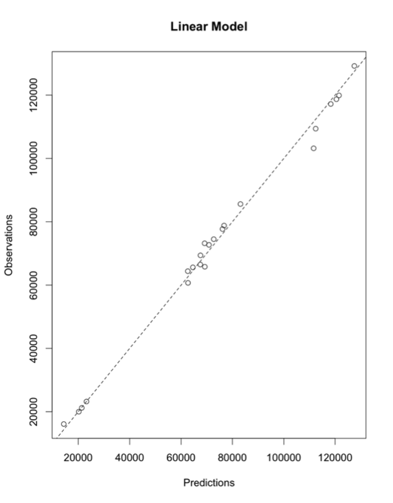
After visually inspecting, we see a really good fit. One of the things to note is that acreage planted is a factor in this model. If there is no difference between acreage planted and acreage harvested, then we aren't really providing more information by looking at storm event frequency. Let's start by looking at the difference between acreage harvested and acreage planted.
Your script should look something like this:
# difference between planted and harvested
differenceHarvestedPlanted <- clean.data$Acreage.Planted-clean.data$Acreage.Harvested
If you now apply the summary function to the difference you will see that although there are instances where no change has occurred between the planted and the harvested, the general difference is between 800-1700 acres. We can also perform a t-test. As a reminder, the t-test will tell us whether the mean acreage planted is statistically different than the mean acreage harvested.
Your script should look something like this:
# perform a t-test
t.test(clean.data$Acreage.Planted,clean.data$Acreage.Harvested,alternative = "two.sided",paired=TRUE)
The result is a P-value <0.01, which means that the mean acreage planted and the acreage harvested are statistically different.
Let's check which variables have statistically significant coefficients in this model (coefficients different from 0)
Your script should look something like this:
# follow up analysis
summary(bestModels[[1]])
We see that the coefficients for the factor variables cold wind chill events, winter storm events, and droughts are statistically significant. The last thing we can do is compare a linear model only using acreage planted (as this is where most of the variability is probably being captured), one which uses acreage planted and the other statistically significant coefficients (cold wind chill events, winter storm events, and droughts), and the one we selected with our automated process.
Your script should look something like this:
# create three separate linear models for comparison
lm.1 <- lm(clean.data$Acreage.Harvested~clean.data$Acreage.Planted)
lm.2 <-
lm(clean.data$Acreage.Harvested~as.numeric(clean.data$Acreage.Harvested)+as.numeric(clean.data$coldWindChill)+as.numeric(clean.data$winterStorm)+as.numeric(clean.data$drought))
lm.3 <- lm(clean.data$Acreage.Harvested~.,lapply(clean.data[,c(1,1+1,7:27)],as.numeric))
If you apply the summary function on all the models you will see that the second model is almost a perfect fit and that lm.3 (which is the best model selected through cross-validation) has a slightly higher R-squared value than lm.1. If we perform an ANOVA analysis between the models, we can determine if the models are statistically different.
Your script should look something like this:
anova(lm.1,lm.2)
anova(lm.1,lm.3)
The results suggest that the change was statistically significant from lm.1 to lm.2. As for the difference between lm.1 and lm.3 (lm.3 is the actual model selected), it is not as strong. This follow-up analysis suggests that it might be best to use linear model 2, which is less complex than linear model 3 but provides a statistically different result from the simple usage of acreage planted. You can see that even though the automation created a good model, by digging in a little more we can further refine it. Data mining is a starting point, not the final solution.
By combining a number of tools you have already learned, we were able to successfully create a model to predict an aspect of the corn harvest effectively. We were able to dig through a relatively large dataset and pull out patterns that could bring added knowledge to investors and farmers, hopefully aiding in better business decisions.