Prioritize...
At the end of this section you should be able to employ tools to choose the best model for your data.
Read...
By now you should know how to create multiple linear regression models as well as regression tree models for any dataset. The next step is to select the best model. Does a regression tree better predict the response variable than a multiple linear regression model? And which response variable can we best predict? Yield/acre, production, acreage harvested? In this section, we will discuss how to evaluate and select the best model.
Predict
Now that we have our models using the multiple linear regression and regression tree approach, we need to use the models to predict. This is the best way to determine how good they actually are. There are multiple ways to go about this.
The first is to use the same data that you trained your model with (when I say train, I mean the data used to create the model). Another option is to break your data up into chunks and use one part of it for training and the other part for testing. For the best results with this option, use the 10-fold cross-validation so that you exploit most of it for training and all of it for testing. The last option is to have two separate datasets: one for training and one for testing. But this will provide a weaker model and should only be used to save time.
Let’s start by predicting our corn production response variables using our multiple linear regression models that were optimized. To do this, I will use the function ‘predict’. Use the code below to predict response variables.
Your script should look something like this:
# create predictions for multiple linear models using the test data (only those with actual lm model results)

lmPredictions.YieldAcre <- predict(lmFinal.YieldAcre,lapply(clean.stateData[,4:12],as.numeric))
lmPredictions.YieldAcre[which(lmPredictions.YieldAcre<0)] <- 0
lmPredictions.Production <- predict(lmFinal.Production,lapply(clean.stateData[,4:12],as.numeric))
lmPredictions.Production[which(lmPredictions.Production < 0)] <- 0
lmPredictions.SeasonAveragePrice <- predict(lmFinal.SeasonAveragePrice,lapply(clean.stateData[,4:12],as.numeric))
lmPredictions.SeasonAveragePrice[which(lmPredictions.SeasonAveragePrice < 0)] <- 0
lmPredictions.ValueofProduction <- predict(lmFinal.ValueofProduction,lapply(clean.stateData[,4:12],as.numeric))
lmPredictions.ValueofProduction[which(lmPredictions.ValueofProduction < 0)] <- 0
lmPredictions.AcreageHarvested <- predict(lmFinal.AcreageHarvested,lapply(clean.stateData[,4:12],as.numeric))
lmPredictions.AcreageHarvested[which(lmPredictions.AcreageHarvested < 0)] <- 0
Because we may have predictions less than 0 which are not plausible for this example, I’ve changed those cases to 0 (the nearest plausible limit). This is a caveat with linear regression. The models are lines and so their output can theoretically extend to plus and minus infinity, well beyond the range of physical plausibility. This means you have to make sure your predictions are realistic. Next, let’s predict the corn production response variables using the optimized regression trees.
Your script should look something like this:
# create predictions for regression tree results
rtPredictions.YieldAcre <- predict(rtFinal.YieldAcre,lapply(clean.stateData[,4:12],as.numeric))
rtPredictions.Production <- predict(rtFinal.Production,lapply(clean.stateData[,4:12],as.numeric))
rtPredictions.SeasonAveragePrice <- predict(rtFinal.SeasonAveragePrice,lapply(clean.stateData[,4:12],as.numeric))
rtPredictions.ValueofProduction <- predict(rtFinal.ValueofProduction,lapply(clean.stateData[,4:12],as.numeric))
rtPredictions.AcreageHarvested <- predict(rtFinal.AcreageHarvested,lapply(clean.stateData[,4:12],as.numeric))
We don’t have to worry about non-plausible results because regression trees are a ‘flow’ chart - not an equation. Now we have predictions for 50 observations and can evaluate the predictions.
Evaluate
To evaluate the models, we are going to compare the predictions to the actual observations. The function regr.eval compares the two and calculates several measures of error that we have used before including the mean absolute error (MAE), mean standard error (MSE), and root mean square error (RMSE). Let’s evaluate the linear models first.
Your script should look something like this:
# use regression evaluation function to calculate several measures of error
lmEval.YieldAcre <- regr.eval(clean.stateData[,"Yield.Acre"],lmPredictions.YieldAcre,train.y=clean.stateData[,"Yield.Acre"]) lmEval.Production <- regr.eval(clean.stateData[,"Production"],lmPredictions.Production,train.y=clean.stateData[,"Production"]) lmEval.SeasonAveragePrice <- regr.eval(clean.stateData[,"Season.Average.Price"],lmPredictions.SeasonAveragePrice,train.y=clean.stateData[,"Season.Average.Price"])
lmEval.ValueofProduction <- regr.eval(subset(clean.stateData[,"Value.of.Production"],!is.na(clean.stateData[,"Value.of.Production"])),subset(lmPredictions.ValueofProduction,!is.na(clean.stateData[,"Value.of.Production"])),train.y=subset(clean.stateData[,"Value.of.Production"],!is.na(clean.stateData[,"Value.of.Production"])))
lmEval.AcreageHarvested <- regr.eval(clean.stateData[,"Acreage.Harvested"],lmPredictions.AcreageHarvested,train.y=clean.stateData[,"Acreage.Harvested"])
There are 6 metrics of which you should already know 3: MAE, MSE, and RMSE. MAPE is the mean absolute percent error – the percentage of prediction accuracy. For the model of yield/acre, the MAPE is 0.11. The predictions were off by 11% on average. MAPE can be biased. NMSE is the normalized mean squared error. It is a unitless error typically ranging between 0 and 1. A value closer to 0 means your model is doing well, while values closer to 1 mean that your model is performing worse than just using the average value of your observations. This is a good metric for selecting which response variable is best predicted. In the yield/acre model, the NMSE is 0.397 while in acreage harvested it is 0.11, suggesting that the acreage harvested is better predicted than yield/acre. The last metric is NMAE, or normalized mean absolute error, which has a value from 0 to 1. For the yield/acre model, the NMAE is 0.59 while in acreage harvested it is 0.32.
Now let’s do the same thing for the regression tree results.
Your script should look something like this:
rtEval.YieldAcre <- regr.eval(clean.stateData[,"Yield.Acre"],rtPredictions.YieldAcre,train.y=clean.stateData[,"Yield.Acre"]) rtEval.Production <- regr.eval(clean.stateData[,"Production"],rtPredictions.Production,train.y=clean.stateData[,"Production"]) rtEval.SeasonAveragePrice <- regr.eval(clean.stateData[,"Season.Average.Price"],rtPredictions.SeasonAveragePrice,train.y=clean.stateData[,"Season.Average.Price"])
rtEval.ValueofProduction <- regr.eval(subset(clean.stateData[,"Value.of.Production"],!is.na(clean.stateData[,"Value.of.Production"])),subset(rtPredictions.ValueofProduction,!is.na(clean.stateData[,"Value.of.Production"])),train.y=subset(clean.stateData[,"Value.of.Production"],!is.na(clean.stateData[,"Value.of.Production"])))
rtEval.AcreageHarvested <- regr.eval(clean.stateData[,"Acreage.Harvested"],rtPredictions.AcreageHarvested,train.y=clean.stateData[,"Acreage.Harvested"])
For the regression tree, the smallest NMSE is with acreage harvested (0.13) similar to the linear model.
Visual Inspection
Looking at the numbers can become quite tedious, so visual inspection can be used. The first visual is to plot the observed values agianst predicted values. Here’s an example for the ‘production’ response variable.
Your script should look something like this:
# visually inspect data
old.par <- par(mfrow=c(1,2))
plot(lmPredictions.Production,clean.stateData[,"Production"],main="Linear Model",
     xlab="Predictions",ylab="Observations")
abline(0,1,lty=2)
plot(rtPredictions.Production,clean.stateData[,"Production"],main="Regression Tree",
     xlab="Predictions",ylab="Observations")
abline(0,1,lty=2)
par(old.par)
You should get a figure similar to this:
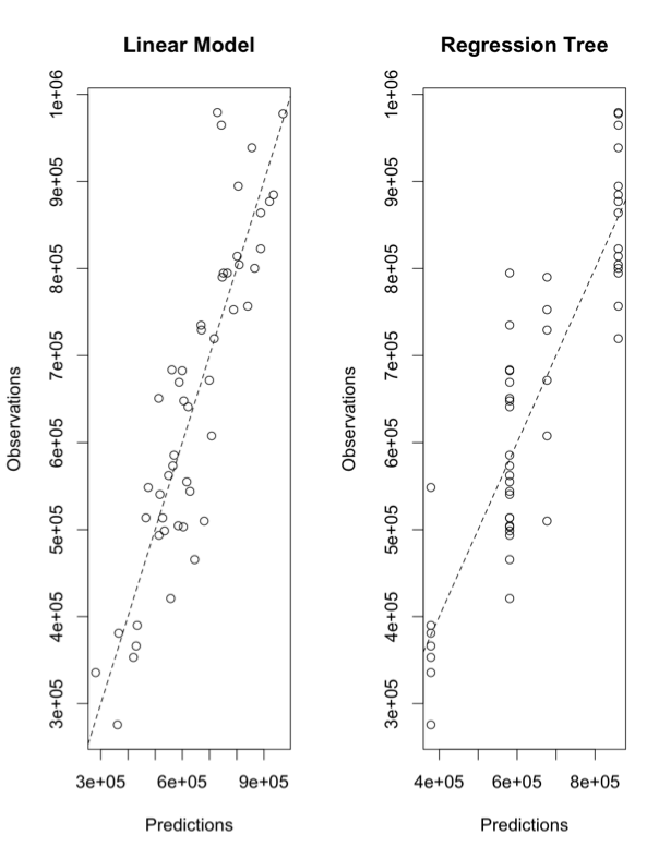
The x-axes for both panels are the predicted values; the y-axes are the observations. The left panel is using the linear model and the right is using the regression tree. The dashed line is a 1-1 line. The linear model does really well, visually, while the regression tree has ‘stacked’ points. This is due to the nature of the ‘flow’ type modeling. There are only a few possible results. In this particular case, there are 4 values as you can see from the tree chart:
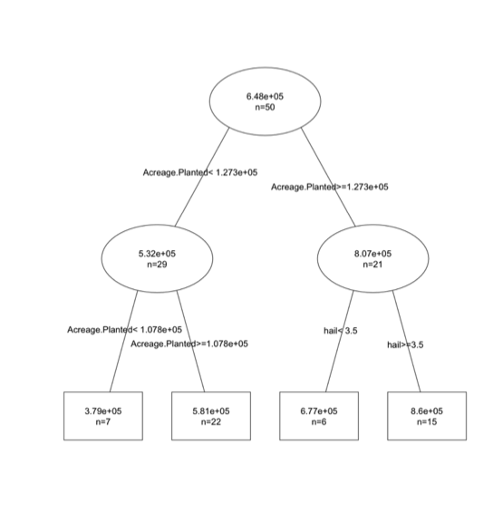
For this particular problem, we are not able to capture the variability as well using the tree. But if the relationship had a discontinuity or was nonlinear, the tree would have won.
Let’s say you notice some poorly predicted values that you want to investigate. You can create an interactive diagram that lets you click on poor predictions to pull out the data. This allows you to look at the observations and predictions, possibly identifying the cause of the problem.
Your script should look something like this:
# interactively click on poor predictions
plot(lmPredictions.Production,clean.stateData[,"Production"],main="Linear Model",
     xlab="Predictions",ylab="Observations")
abline(0,1,lty=2)
clean.stateData[identify(lmPredictions.Production,clean.stateData[,"Production"]),]
Doing this for every single model, especially when you have several response variables, can be tedious. So how can we compare all the model types efficiently?
Model Comparison
When it comes to data mining, the goal is to be efficient. When trying to choose between types of models as well as which response variable we can best predict, automating the process is imperative. To begin, we are going to set up functions that automate the processes we just discussed: create a model, predict the model, and calculate a metric for comparison. The code below creates two functions: one using the multiple linear regression approach and one with the regression tree approach.
# create function to train test and evaluate models through cross-validation
cvRT <- function(form,train,test,...){
  modelRT<-rpartXse(form,train,...)
  predRT <- predict(modelRT,test)
  predRT <- ifelse(predRT <0,0,predRT)
  mse <- mean((predRT-resp(form,test))^2)
  c(nmse=mse/mean((mean(resp(form,train))-resp(form,test))^2))
}
cvLM <- function(form,train,test,...){
  modelLM <- lm(form,train,...)
  predLM <- predict(modelLM,test)
  predLM <- ifelse(predLM <0,0,predLM)
  mse <- mean((predLM-resp(form,test))^2)
  c(nmse=mse/mean((mean(resp(form,train))-resp(form,test))^2))
}
Let’s break the first function (cvRT) down.
You supply the function the form of the model you want, response variables~factor variables. You then supply the training data and the testing data. When this function is called, it uses the same function we used before ‘rpartXse’. Once the optimal regression tree is created, the function predicts the values using the optimized model (modelRT) and the test data. We then replace any nonsensical values (less than 0) with 0. Then we calculate NMSE and save the value. This is the value we will use for model comparison.
The second function (cvLM) is exactly the same, but instead of using the regression tree approach we use the multiple linear regression approach.
Once the optimal models for each response variable are selected (one for each approach), we want to select the approach that does a better job. To do this, we are going to use the function ‘experimentalComparison’. This function implements a cross-validation method. With this function, we need to supply the datasets (form, train, test) and the parameter called ‘system’. These are the types of models you want to run (cvLM and CVRT). Here is where you would supply any more parameters you may want to use. For example, in the function rpartXse we can assign thresholds like the number of splits or the cp. The last parameter is cvSettings. These are the settings for the cross-validation experiment. It is in the form of X, K, Z where X is the number of times to perform the cross-validation process, K is the number of folds (the number of equally sized subsamples), and Z is the seed for the random number generator. Let’s give this a try for the acreage harvested response variable.
Your script should look something like this:
# perform comparison
results <- experimentalComparison(
  c(dataset(Acreage.Harvested~.,lapply(clean.stateData[,c(4,5,10:12)],as.numeric),'Acreage.Harvested')),
  c(variants('cvLM'), variants('cvRT',se=c(0,0.5,1))),
  cvSettings(3,10,100))
For the regression tree, I added the parameter SE=0, 0.5, and 1. Remember, SE is xerror+xstd. But in reality there is a coefficient in front of xstd, given by the numbers used in this setting (0, 0.5 and 1). This setting will create three random forests with varying SE threshold (xerror, xerror+0.5xstd, xerror+1*xstd). I set ‘cvSettings’ to 3,10,100 which means we are going to run a 3-10 Fold cross-validation. We want 3 iterations chunking the data into 10 equally sized groups. We set the random number generator to 100.
Why do we run iterations? It provides statistics on the performance metric! Let’s take a look by summarizing the results.
Your script should look something like this:
# summarize the results
summary(results)
The output begins by telling us the type of cross-validation that was used, in this case 3X10. It also tells us the seed for the random number generator. Next, the data sets are displayed followed by four learners (model types): one version of a linear model and three versions of a regression tree (se=0,0.5, and 1). Next is the summary of the results, which are broken down by the learner (model). We only saved the metric NMSE, so that is the only metric we will consider. You can change this depending on what you are interested in, but with respect to comparing models the NMSE is a pretty good metric. The NMSE for each learner, the average, the std, the min, and the maximum are computed. This can be done because of the cross-validation experiment! Because we ran it 3 times with 10 folds (10 chunks of data) we can create statistics on the error of the model. For this case, it appears the linear model is the best as it has the lowest average NMSE.
If we want to visualize these results, we can run the following code:
Your script should look something like this:
# plot the results
plot(results)
You should get a figure similar to this:
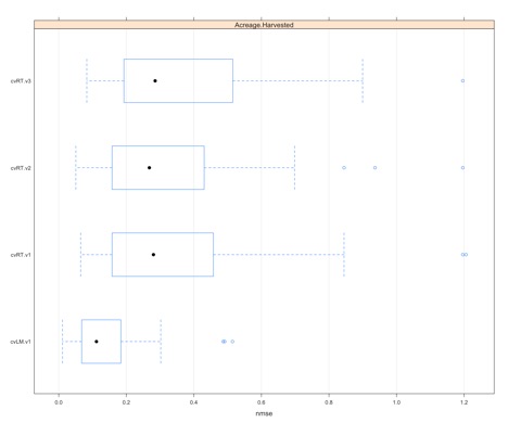
This creates a boxplot of the NMSE values estimated for each iteration and fold (30 total points). It’s a good way to visually determine which model type is best for this particular response variable as well as display the spread of the error.
Ensemble Model and Automation
We now want to take the automation to another level. We want to be able to create models for all the response variables, not just one. To do this, we need to create a list that contains the form of each model. Use the code below:
Your script should look something like this:
# apply function for all variables to predict
dataForm <- sapply(names(clean.stateData)[c(5:9)],
                   function(x,names.attrs){
                                           f <- as.formula(paste(x,"~."))
                                           dataset(f,lapply(clean.stateData[,c(names.attrs,x)],as.numeric),x)
                                           },
                   names(clean.stateData)[c(4,10:12)])
dataForm is a list variable that contains the datasets needed for the experimental comparison: form, train, and test. Now we can automate the whole process.
Your script should look something like this:
allResults <- experimentalComparison(dataForm,
                                    c(variants('cvLM'),variants('cvRT',se=c(0,0.5,1))),
                                    cvSettings(5,10,100))
Notice that this time I’ve decided to perform a 5x10 cross-validation process. This might take a bit longer to run, so be patient.
Now let’s plot the results to get a visual.
Your script should look something like this:
# plot all results
plot(allResults)
You should get the following figure:
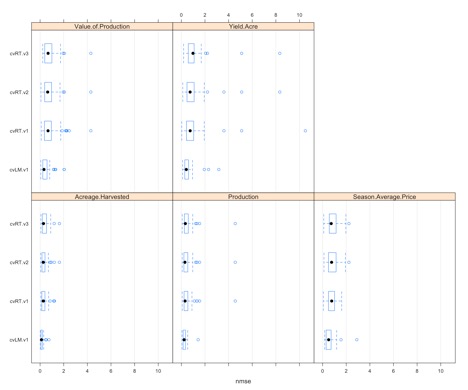
Each panel represents one of the response variables we want to predict. Within each panel, we see a boxplot for the four learners (the one linear model and the 3 regression trees). In this case, we have 50 estimates of NMSE going into the boxplot. We will see that some variables, like acreage harvested or yield/acre, might have an obvious model selection, but for others it's unclear. We can use the function ‘bestscores’ to select the model with the smallest average NMSE for each response variable.
Your script should look something like this:
# determine the best scores
bestScores(allResults)
For this example, the linear model is actually chosen for all response variables. And acreage harvested has the smallest overall NMSE, suggesting that acreage harvested might be the corn response variable we should focus on.
There is one more type of model that we should discuss. In addition to regression trees and linear regression models we can create a random forest. A random forest is an example of an ensemble model. Ensembles are the combinations of several individual models that at times are better at predicting than their individual parts. In this case, a random forest is an ensemble of regression trees. Let’s begin by creating a function to compute the random forest
# now create a random forest (ensemble model)
library(randomForest)
cvRF <- function(form,train,test,...){
  modelRF <- randomForest(form,train,...)
  predRF <- predict(modelRF,test)
  predRF <- ifelse(predRF <0,0,predRF)
  mse <- mean((predRF-resp(form,test))^2)
  c(nmse=mse/mean((mean(resp(form,train))-resp(form,test))^2))
}
Similar to the other model methods, we need a dataset with the form, train, and test inputs. We then use the experimental comparison but add in our new learner- cvRF.
Your script should look something like this:
allResults <- experimentalComparison(dataForm,
                                     c(variants('cvLM'), variants('cvRT',se=c(0,0.5,1)),
                                       variants('cvRF',ntree=c(70,90,120))),
                                     cvSettings(5,10,100))
The ntree parameter tells the random forest how many individual trees to create. You want a large enough number of individual trees to create a meaningful result but small enough to be computationally efficient. Here’s an article, "How Many Trees in a Random Forest?," that says the number should be between 64 and 128. If the function is taking too long to run, you probably have too many trees.
Let’s run the code with the random forest included and determine the best scores.
Your script should look something like this:
# look at scores
bestScores(allResults)
After running this, you will notice that now we have some random forests listed as the best models instead of only the linear regression model.