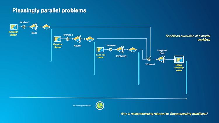
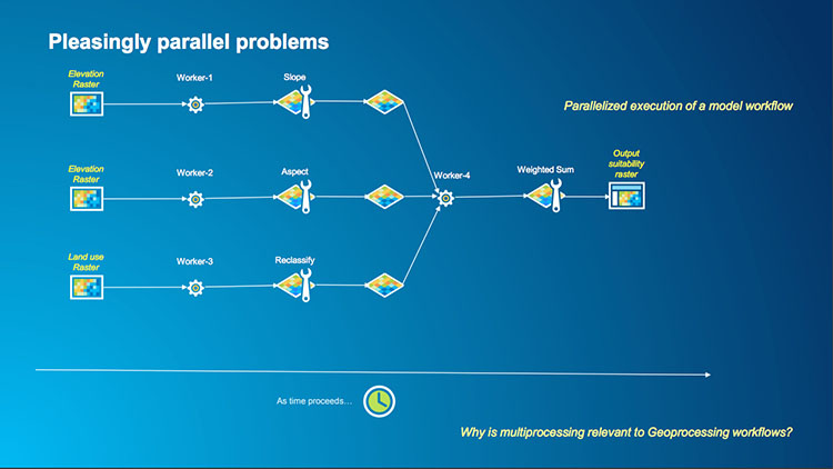
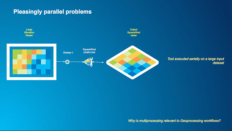
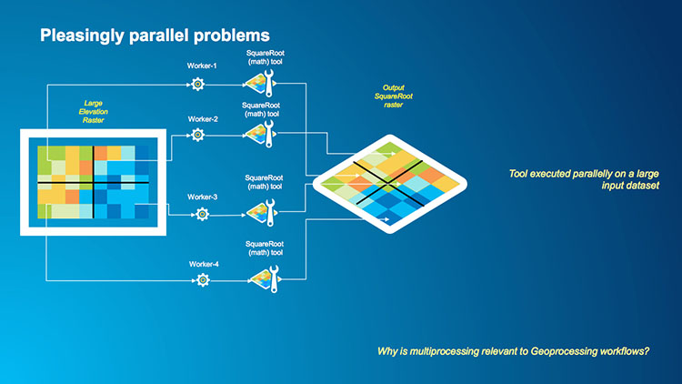
There are two types of operations with rasters that can easily (and productively) be implemented in parallel: operations that are independent components in a workflow, and raster operations which are local, focal or zonal – that is they work on a small portion of a raster such as a pixel or a group of pixels.
Esri’s Clinton Dow and Neeraj Rajasekar presented way back at the 2017 User Conference demonstrating multiprocessing with arcpy and they had a number of useful graphics in their slides which demonstrate these two categories of raster operations which we have reproduced here as they're still appropriate and relevant.
An example of an independent workflow would be if we calculate the slope, aspect and some other operations on a raster and then produce a weighted sum or other statistics. Each of the operations is independently performed on our raster up until the final operation which relies on each of them (see the first image below). Therefore, the independent operations can be parallelized and sent to a worker and the final task (which could also be done by a worker) aggregates or summarises the result. Which is what we can see in the second image as each of the tasks is assigned to a worker (even though two of the workers are using a common dataset) and then Worker 4 completes the task. You can probably imagine a more complex version of this task where it is scaled up to process many elevation and land-use rasters to perform many slope, aspect and reclassification calculations with the results being combined at the end.


An example of the second type of raster operation is a case where we want to make a mathematical calculation on every pixel in a raster such as squaring or taking the square root. Each pixel in a raster is independent of its neighbors in this operation so we could have multiple workers processing multiple tiles in the raster and the result is written to a new raster. In this example, instead of having a single core serially performing a square root calculation across a raster (the first image below) we can segment our raster into a number of tiles, assign each tile to a worker and then perform the square root operation for each pixel in the tile outputting the result to a single raster which is shown in the second image below.


Bearing in mind the caveats about parallel programming from above and the process that we undertook to convert the Hi Ho Cherry-O program, let's begin.
The DEM that we will be using can be downloaded and the sample code is below that we want to conver it is below.
# This script uses map algebra to find values in an
#  elevation raster greater than 3500 (meters).

import arcpy
from arcpy.sa import *

# Specify the input raster
inRaster = arcpy.GetParameterAsText(0)
cutoffElevation = arcpy.GetParameter(1)
outPath = arcpy.env.workspace

# Check out the Spatial Analyst extension
arcpy.CheckOutExtension("Spatial")

# Make a map algebra expression and save the resulting raster
outRaster = Raster(inRaster) > cutoffElevation
outRaster.save(outPath+"/foxlake_hi_10")

# Check in the Spatial Analyst extension now that you're done
arcpy.CheckInExtension("Spatial")
Our first task is to identify the parts of our problem that can work in parallel and the parts which we need to run sequentially.
The best place to start with this can be with the pseudocode of the original task. If we have documented our sequential code well, this could be as simple as copying/pasting each line of documentation into a new file and working through the process. We can start with the text description of the problem and build our sequential pseudocode from there and then create the multiprocessing pseudocode. It is very important to correctly and carefully design our multiprocessing solutions to ensure that they are as efficient as possible and that the worker functions have the bare minimum of data that they need to complete the tasks, use memory workspaces, and write as little data back to disk as possible.
Our original task was :
Get a list of raster tiles
For every tile in the list:
     Fill the DEM
     Create a slope raster
     Calculate a flow direction raster
     Calculate a flow accumulation raster
     Convert those stream rasters to polygon or polyline feature classes.
You will notice that I’ve formatted the pseudocode just like Python code with indentations showing which instructions are within the loop.
As this is a simple example we can place all of the functionality within the loop into our worker function as it will be called for every raster. The list of rasters will need to be determined sequentially and we’ll then pass that to our multiprocessing function and let the map element of multiprocessing map each raster onto a worker to perform the tasks. We won’t explicitly be using the reduce part of multiprocessing here as the output will be a featureclass but reduce will probably tidy up after us by deleting temporary files that we don’t need.
Our new pseudocode then will look like :
Get a list of raster tiles
For every tile in the list:
    Launch a worker function with the name of a raster
Worker:
Fill the DEM
     Create a slope raster
     Calculate a flow direction raster
     Calculate a flow accumulation raster
     Convert those stream rasters to polygon or polyline feature classes.
Bear in mind that not all multiprocessing conversions are this simple. We need to remember that user output can be complicated because multiple workers might be attempting to write messages to our screen at once and that can cause those messages to get garbled and confused. A workaround for this problem is to use Python’s logging library which is much better at handling messages than us manually using print statements. We haven't implemented logging in this sample solution for this script but feel free to briefly investigate it to supplement the print and arcpy.AddMessage functions with calls to the logging function. The Python Logging Cookbook has some helpful examples.
As an exercise, attempt to implement the conversion from sequential to multiprocessing. You will probably not get everything right since there are a few details that need to be taken into account such as setting up an individual scratch workspace for each call of the worker function. In addition, to be able to run as a script tool the script needs to be separated into two files with the worker function in its own file. But don't worry about these things, just try to set up the overall structure in the same way as in the Hi Ho Cherry-O multiprocessing version and then place the code from the sequential version of the raster example either in the main function or worker function depending on where you think it needs to go. Then check out the solution linked below.
Click here for one way of implementing the solution
When you run this code, do you notice any performance differences between the sequential and multiprocessor versions?
The sequential version took 96 seconds on the same 4-processor PC we were using in the Cherry-O example, while the multiprocessor version completed in 58 seconds. Again not 4 times faster as we might expect but nearly twice as fast with multiprocessing is a good improvement. For reference, the 32-processor PC from the Cherry-O example processed the sequential code in 110 seconds and the multiprocessing version in 40 seconds. We will look in more detail at the individual lines of code and their performance when we examine code profiling but you might also find it useful to watch the CPU usage tab in Task Manager to see how hard (or not) your PC is working.
Lesson content developed by Jan Wallgrun and James O’Brien