Hypothesis Formation and Testing for 1 Sample: Part 2

Read...

Decision Rules

Now that we have the hypothesis stated and have chosen the level of significance we want, we need to determine the decisions rules. In particular, we need to determine threshold value(s) for the test statistic beyond which we can reject the null hypothesis. There are two ways to go about this: the P-Value approach and the Critical Value approach. These approaches are equivalent, so you can decide which one you like the most.

The P-value approach determines the probability of observing a value of the test statistic more extreme than the threshold assuming the null hypothesis is true; you look at the probability of the test statistic value you calculated from your data. For the P-value approach, we compare the probability (P-value) of the test statistic to the significance level (α). If the P-value is less than or equal to α, then we reject the null hypothesis in favor of the alternative hypothesis. If the P-value is greater than α, we do not reject the null hypothesis. Here is the region of rejection of the null hypothesis for a one-sided and two sided test:

• If H₁: μ<μ_o (Lower Tailed Test) and the probability from the test statistic is less than α, then the null hypothesis is rejected, and the alternative is accepted.
• If H₁: μ>μ_o (Upper Tailed Test) and the probability from the test statistic is less than α, then the null hypothesis is rejected, and the alternative is accepted.
• If H₁: μ≠μ_o (Two Tailed Test) and the probability from the test statistic is less than α/2, then the null hypothesis is rejected, and the alternative is accepted.

For the P-value approach, the direction of the test (lower tail/upper tail) does not matter. If the probability is less than α (α/2 for a two-tailed test), then we reject the null hypothesis.

The critical value approach looks instead at the actual value of the test statistic. We transform the significance level, α, to the test statistic value. This requires us to be very careful about the direction of the test. If your test statistic lies beyond the critical value, then reject the null hypothesis. Let's break it down by test:

If H₁: μ<μ_o (Lower Tailed Test):

Simply find the corresponding test statistic value of the assigned significance level (α); that is, if α is 0.05 find the t or Z-value that corresponds to a probability of 0.05. This is your critical value and we denote this as Z_α or t_α.

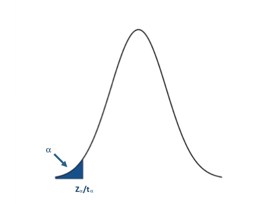
The blue shaded area represents the rejection region. For the lower tailed test, if the test statistic is to the left of the critical value (less than) in the rejection region (blue shaded area), we reject the null hypothesis. I said before that one common α value was 0.05 (a 5% chance of a type I error). For α=0.05, the corresponding Z-value would be -1.645. The Z-statistic would have to be less than -1.645 for the null hypothesis to be rejected at the 95% confidence level.

If H₁: μ>μ_o (Upper Tailed Test):

You have to remember that the t and Z-values use the CDFs of the PDF. This means that for the right tail or upper tail the corresponding t and Z-values will actually come from 1-α. For example, if α is 0.05 and we have an upper tail test, we find the t or Z-value that corresponds to a probability of 0.95. This would be the critical value and we denote this as Z_1-α or t_1-α.

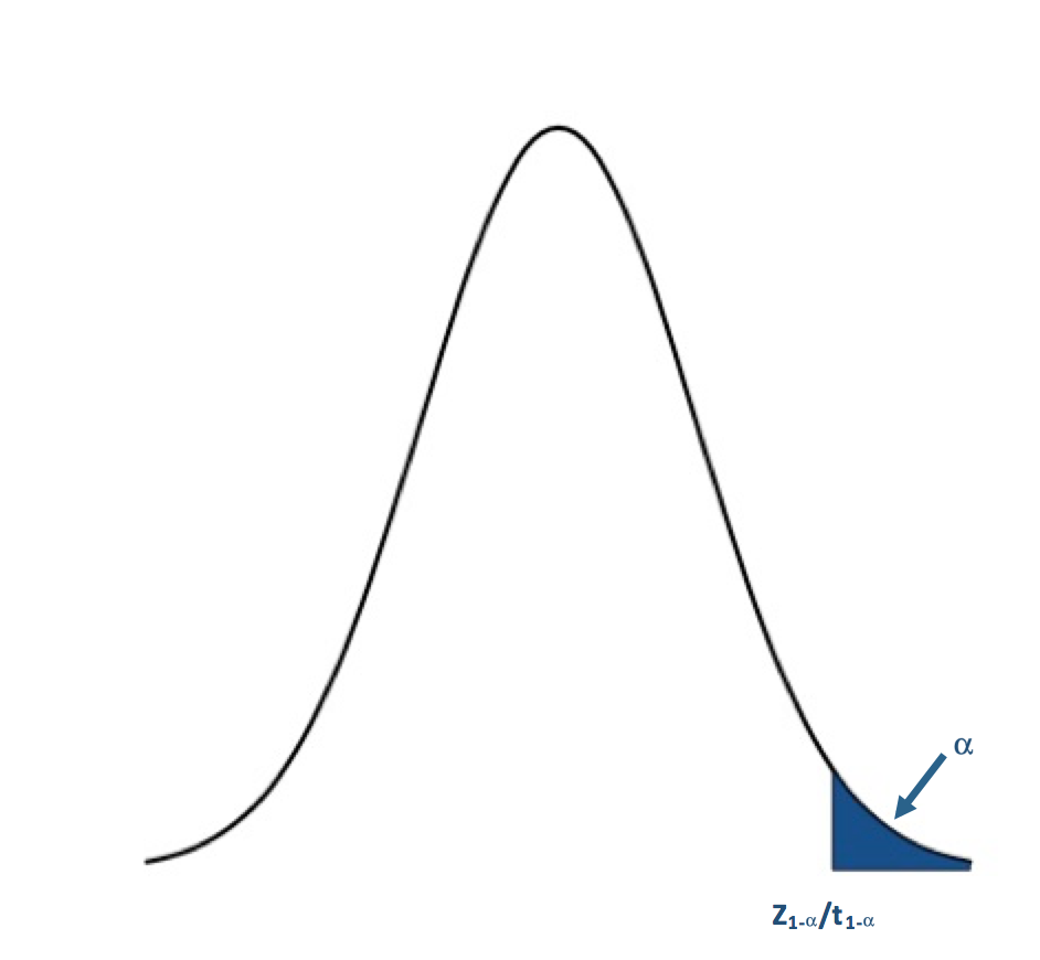
For the upper tailed test, if the test statistic is to the right of the critical value (greater than), we reject the null hypothesis. For α=0.05, the corresponding Z-value would be 1.645. The Z-statistic would have to be greater than 1.645 for the null hypothesis to be rejected at the 95% confidence level.

If H₁: μ≠μ_o (Two Tailed Test):

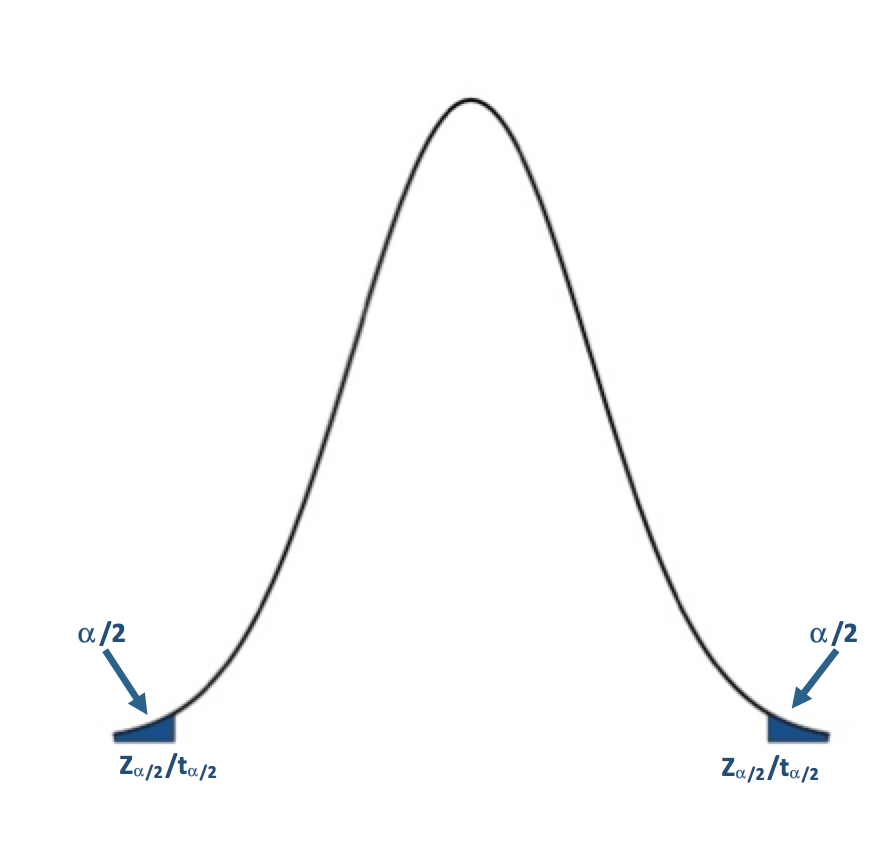
For the two-tailed test, if your test statistic is to the left of the lower critical value or the right of the upper critical value, then we reject the null hypothesis. For α=0.05, the corresponding Z-value would be ±1.96. The Z-statistic would have to be less than -1.96 or greater than 1.96 for the null hypothesis to be rejected at the 95% confidence level.

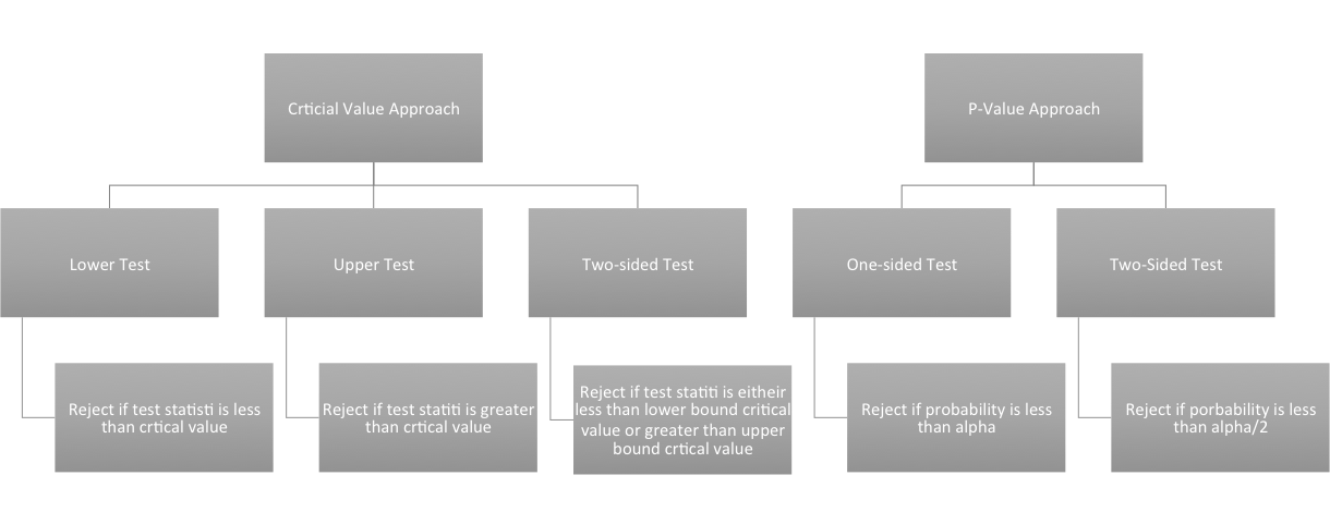
I suggest that for nonparametric tests, such as the Wilcoxon or Sign test, that you use the P-value approach because the functions available in R will estimate the P-value for you which means you do not have to estimate the critical value for these tests, avoiding a tedious task. Here is a flow chart for the rejection of the null hypothesis. Here is a larger view (opens in another tab).

Computation and Confidence Interval

Finally, after we have set up the hypothesis and determine our significance level, we can actually compute the test statistic. In this section, I will briefly talk about functions available in R to calculate the Z, t, Wilcoxon, and the Sign test statistics. But first, I want to talk about confidence intervals. Confidence intervals are estimates of the likely range of the true value of a particular parameter given the estimate of that parameter you've computed from your data. For example, confidence intervals are created when estimating the mean of the population. This confidence interval represents a range of certainty our data gives us about the population mean; we are never 100% certain the mean of a sample dataset represents the true mean of a population, so we calculate the range in which the true mean lies within with a certain confidence. Most times confidence intervals are set at the 95% or 99% level. This means we are 95% (99%) confident that the true mean is within the interval range. To estimate the confidence interval, we create a lower and upper bound using a Z-score reflective of the desired confidence level:

$$\left(\overline{x}-z\ast \frac{\sigma }{\sqrt{n}},\overline{x}+z\ast \frac{\sigma }{\sqrt{n}}\right)$$

where $\overline{x}$ is the estimated mean from the dataset, σ is the estimate of the standard deviation of the dataset, n is the sample size, and z is the Z-score representing the confidence level you want. The common confidence levels of 95% and 99% have Z-scores of 1.96 and 2.58 respectively. You can estimate a confidence interval using t-scores instead if n is small, but the t-values depend on the degrees of freedom (n-1). You can find t-scores at any confidence level using this table. Confidence intervals, however, can be calculated in R by supplying only the confidence level as a percentage; generally, you will not have to determine the t-score yourself.

For the Z-test, you can just calculate the Z-score yourself or you can use the function "z.test" from the package "BSDA". This function can be used for testing two datasets against each other, which will be discussed further on in this section. For now, let's focus on how to use this function for one dataset. There are 5 arguments for this function that are important:

• The first is "x", which is the dataset you want to test. You must remove NaNs, NAs, and Infs from the dataset. One way to do this is use "na.omit".
• The second argument is "alternative", which is a character string. "Alternative" can be assigned "greater", "less", or "two.sided". This refers to the type of test you are performing (one-sided upper, one-sided lower, or two-sided).
• The third argument is "mu" which is the mean stated in the null hypothesis. This value will be the μ_o from the hypothesis statement.
• "Sigma.x" is the standard deviation of the dataset. You can calculate this using the function "sd"; again you must remove any NaNs, NAs, or Infs.
• Lastly, the argument "conf.level" is the confidence level for which you want the confidence interval to be calculated. I would recommend using a confidence level equal to 1-α. If you are interested in a significance level of 0.05, then the conf.level will be set to 0.95.

The great thing about the function "z.test" is that it provides both the Z-value and the P-value so you can use either the critical value approach or the P-value approach. The function will also provide a confidence interval for the population. Note that if you use a one-sided test, your confidence interval will be unbounded on one side.

When the data is normally distributed but the sample size is small, we will use the t-test, or the function "t.test" in R. This function has similar arguments to the "z.test".

• The first is "x" which again is the dataset.
• The next argument is "alternative" which is identical to the "z.test", set to "two.sided", greater," or "less".
• Next is "mu" which again is set to μ_o in the hypothesis statement.
• The argument "conf.level" is the confidence level for the confidence interval.
• Lastly, there is an argument "na.action" that can be set to "TRUE" which would omit NaNs and NAs from the dataset, meaning you do not have to use "na.omit".

Similar to the "z.test", the "t.test" provides both the t-value and the P-value, so you can either use the critical value approach or the P-value approach. It will also automatically provide a confidence interval for the population mean. Again, if you use a one-sided test your confidence interval will be unbounded on one side.

The 'z.test' and 't.test' are for data that is parametric. What about nonparametric datasets - ones in which we do not have parameters to represent the fit? I'm only going to show you the functions for the Wilcoxon test and the Sign test which I described previously. There are, however, many other test statistics you can calculate using functions available in R.

The Wilcoxon test or 'wilcox.test' in R, which is used for nonparametric cases that appear symmetric, has similar arguments as the 'z.test'.

• You first must provide 'x' which is the dataset.
• 'Alternative' describes the type of test i.e., "less", "greater", or "two-sided".
• Next, you provide "mu" which generally is the median value in the hypothesis, η_o.
• This function will also create a confidence interval for the estimate of the median. To do this, provide the 'conf.level' as well as set 'conf.int' equal to "TRUE".

The test provides a P-value as well as a critical value, but I would recommend for nonparametric tests to follow the P-value approach because of the tediousness in estimating the critical value.

For the sign test use the function 'SIGN.test' in R. The arguments are:

• 'x' which is the dataset,
• 'md' which is the median value, η_o, from the hypothesis,
• 'alternative' which is the type of test, and lastly
• 'conf.level' which is the confidence level for the estimate of the confidence interval of the median.

Again, the test provides a P-value as well as a critical value, but I would recommend for nonparametric tests to follow the P-value approach.

Decision and Interpretation

The last step in hypothesis testing is to make a decision based on the test statistic and interpret the results. When making the decision, you must remember that the testing is of the null hypothesis; that is, we are deciding whether to reject the null hypothesis in favor of the alternative. The critical region changes depending on whether the test is one-sided or two-sided; that is, your area of rejection changes. Let’s break it down by two-sided, upper, and lower. Note that I will write the results with respect to the Z-score, but the decision is the same for whatever test statistic you are using. Simply replace the Z-value with the value from your test statistic.

For a two-tailed test, your hypothesis statement would be:

$$H_o:\mu ={\mu }_o$$ $$H_1:\mu \ne {\mu }_o$$

You will reject the null hypothesis (H_o) and accept the alternative (H₁) if:

• the probability from the test statistic is less than α/2 or
• the Z-score is less than -Z_α/2 or greater than +Z_α/2
  • For Nonparametric data, this critical value will not be symmetric, i.e., you must calculate the critical value for the lower bound (α/2) and the upper bound (1-α/2)

For an upper one-tailed test, your hypothesis statement would be:

$$H_o:\mu \le {\mu }_o$$$$H_1:\mu >{\mu }_o$$

You will reject the null hypothesis (H_o) and accept the alternative (H₁) if:

• the probability from the test statistic is less than α or
• the Z-score is greater than Z_1-α

For a lower one-tailed test, your hypothesis statement would be:

$$H_o:\mu \ge {\mu }_o$$$$H_1:\mu <{\mu }_o$$

You will reject the null hypothesis (H_o) and accept the alternative (H₁) if:

• the probability from the test statistic is less than α or
• the Z-score is less than Z_α

Again, for any other test (t-test, Wilcox, or Sign), simply replace the Z-value and Z-critical values with the corresponding test values.

So, what does it mean to reject or fail to reject the null hypothesis? If you reject the null hypothesis, it means that there is enough evidence to reject the statement of the null hypothesis and accept the alternative hypothesis. This does not necessarily mean the alternative is correct, but that the evidence against the null hypothesis is significant enough (1-α) that we reject it for the alternative. The test statistic is inconsistent with the null hypothesis. If we fail to reject the null hypothesis, it means the dataset does not provide enough evidence to reject the null hypothesis. It does not mean that the null hypothesis is true. When making a claim stemming from a hypothesis test, the key is to make sure that you include the significance level of your claim and know that there is no such thing as a sure thing in statistics. There will always be uncertainty in your result, but understanding that uncertainty and using it to make meaningful decisions makes hypothesis testing effective.

Now, give it a try yourself. Below is an interactive tool that allows you to perform a one-sided or two-sided hypothesis test on temperature data for London. You can pick whatever threshold you would like to test, the level of significance, and the type of test (Z or t). Play around and take notice of the subtle difference between the Z and t-tests as well as how the null and alternative hypothesis are formed.