Hypothesis Formation and Testing for 1 Sample: Part 1

Read...

Let's say you think BBQ sales triple when the temperature exceeds 20°C in Scotland. How would you test that? Well one way is through hypothesis testing. Hypothesis generation and testing can seem confusing at times. This section will contain a lot of potentially new terminology. The key for success in this section is to know the terms; know exactly what they mean and how to interpret them. Working through examples will be extremely beneficial. There will be an entire section filled with examples. Take the time now to understand the terminology.

Here is a general overview of hypothesis formation and testing. This is meant to be a basic procedure which you can follow:

1. State the question.
2. Select the null and alternative hypothesis.
3. Check basic assumptions.
4. Identify the test statistic.
5. Specify the level of significance.
6. State the decision rules.
7. Compute the test statistics and calculate confidence intervals.
8. Make decision about rejecting null hypothesis and interpret results.

State the Question

Stating the question is an important part of the process when it comes to hypothesis testing. You want to frame a question that answers something you are interested in but also is something that you can answer. When coming up with questions, try and remember that the basis of hypothesis testing is the formation of a null and alternative hypothesis. You want to frame the question in a way that you can test the possibility of rejecting a claim. 

Selection of the Null Hypothesis and Alternative Hypothesis

When selecting the null and alternative hypothesis, we use the question that we stated and formulate the hypotheses based on questioning the null hypothesis. A common example of a hypothesis is to determine whether an observed target value, μ_o, is equal to the population mean, μ. The hypothesis has two parts, the null hypothesis and the alternative hypothesis. The null hypothesis (H_o) is the statement we will test. Through hypothesis testing, we are trying to find evidence against the null hypothesis. The null hypothesis is what we are trying to disprove or reject. The alternative hypothesis (H₁ sometimes H_A) states the other alternative - it's usually what think to be true. The two are mutually exclusive and together cover all possible outcomes. The alternative hypothesis is what you speculate to be true and is the opposite of the null hypothesis.

There are three ways to format the hypothesis depending on the question being asked: two tailed test, upper tailed test (right tailed test), and the lower tailed test (left tailed test). For the two tailed test, the null hypothesis states that the target value (μ_o) is equal to the population mean (μ). We would write this as:

$$H_0:\mu ={\mu }_o$$

The alternative hypothesis is that the null hypothesis is not true. We would write it as:$$H_1:\mu \ne {\mu }_o$$

An example would be that we want to know whether the total amount of rain that fell this month is unusual.

The upper tailed test is an example of a one-sided test. For the upper tailed test, we speculate that the population mean (μ) is greater than the target value (μ_o). This might seem backwards, but let’s write it out first. The null hypothesis would be that the population mean (μ) is less than or equal to the target value (μ_o):

$$H_0:\mu \le {\mu }_o$$

And the alternative hypothesis would be that the population mean (μ) is greater than the target value (μ_o):

$$H_1:\mu >{\mu }_o$$

It’s called the upper tailed test because we are examining the likelihood of the sample mean being observed in the upper tail of the distribution if the null hypothesis were true. In this case, the null hypothesis is that the target value (μ_o) is equal to or greater than the population mean (μ); it lies in the upper tail. An example would be that the temperature today feels unusually cold for the month. We are hoping to reject that the temperature is actually warmer than the usual.

The lower tailed test is also an example of a one-sided test. For the lower tailed test, we speculate that the target value (μ_o) is greater than the population mean (μ). Again, let's write this out. The null hypothesis would be that the target value (μ_o) is less than or equal to the population mean (μ):

$$H_0:\mu \ge {\mu }_o$$

And the alternative hypothesis would be that the target value (μ_o) is greater than the population mean (μ):$$H_1:\mu <{\mu }_o$$

This is called the lower tailed because we are testing whether the target value (μ_o) is less than the population mean (μ); we are testing that the target value (μ_o) lies in the lower tail. An example would be that the wind feels unusually gusty today. We speculate that the wind is gusty. We want to reject that the wind is lower than usual, so we test whether it is in the lower tail or not.

For now, all you need to know is how to form the null hypothesis and alternative hypothesis and whether this results in a two-sided or one-sided test (lower or upper). Knowing the type of test will be important when determining the decision rules. Here is a summary:

Speculate that the population mean is simply not equal to the target value:

• Two-Tailed Test
  $$\begin{array}{l}{H}_0:\mu ={\mu }_o\\ H_1:\mu \ne {\mu }_o\end{array}$$

Speculate that the value is less than the mean:

• One-Tailed Test: Upper
  $$\begin{array}{l}{H}_0:\mu \le {\mu }_o\\ H_1:\mu >{\mu }_o\end{array}$$

Speculate that the value is greater than the mean:

• One-Tailed Test: Lower
  $$\begin{array}{l}{H}_0:\mu \ge {\mu }_o\\ H_1:\mu <{\mu }_o\end{array}$$

For nonparametric testing, the null and alternative hypothesis are stated the same way. Both one-tailed and two tailed tests can be performed. The main difference is that generally the median is considered instead of the mean.

Basic Assumptions

There are several assumptions made when hypothesis testing. These assumptions vary depending on the type of hypothesis test you are interested in, but the assumptions will usually involve the level of measurement error of the variable, the method of sampling, the shape of the population distribution, and the sample size. If you check these assumptions, you should be able to determine whether your data is suitable for hypothesis testing.

All hypothesis testing requires your data to be an independent random sample. Each draw of the variable must be independent of each other; otherwise hypothesis testing cannot proceed. If your data is an independent random sample, then you can continue on. The next question is whether your data is parametric or not. Parametric data is data that is fit by a known distribution so you can use the set of hypothesis tests specific to that distribution. For example, if the data is normally distributed then the data meets the requirements for hypothesis testing using that distribution and you can continue with the associated procedures. For non-normally distributed data, you can invoke the central limit theory. If this does not work, you can transform to normal, use the parametric test appropriate to the distribution your data is fit by, or use a nonparametric test. In any case, at that point your data meets the requirements for hypothesis testing and you can continue on. If your data is non-normally distributed, has a small sample size, and cannot be transformed, you will have switch to the nonparametric testing methods which will be discussed later on. The caveat about nonparametric test statistics is that, because they make no assumptions about the underlying probability distributions, the results are less robust. Below is an interactive flow chart you can use to help you determine whether your data meets the requirements for hypothesis testing.  Here is a larger, static view.

Test Statistics

Once we have stated the hypotheses, we must choose a test statistic appropriate to our null hypothesis. We can calculate any statistic from our sample data and there is more than one test to allow us to see how likely it is that the population value is different from some target. For this lesson, we are going to focus specifically on the means. There are two test statistics for data that are either normally distributed or numerous enough that we can invoke the central limit theory. The first is the Z-test. The Z-test is the same as the Z-score:

$$z=\frac{x-\mu }{\frac{\sigma }{\sqrt{n}}}$$

X is the target value (μ_o from the hypothesis statement), μ is the population mean, σ is the population standard deviation, and n is the number of samples. When we use the Z-test, we assume that the number of samples is sufficiently large enough so that the sample mean and standard deviation are representative of the population mean and standard deviation. We use a Z-table to determine the probability associated with the Z-statistic value calculated from our data. The Z-test can be used for both one-sided and two sided tests.

If we have a small dataset (less than 30), then we will need to perform a t-test instead. The main difference between the t-test and the Z-test is that in the Z-test we assume that the standard deviation of the data (the sample standard deviation) represents the population standard deviation, because the sample size is large enough (greater than 30). If the sample size is small, the standard deviation of the dataset does not represent the population standard deviation. We therefore have to assume a t-distribution. The test statistic itself is calculated exactly the same as the Z-statistic:

$$t=\frac{x-\mu }{\frac{\sigma }{\sqrt{n}}}$$

The difference is that we use a t-table to determine the corresponding probability. The probabilities in the t-table vary with the number of cases in the dataset, so that they approach the probabilities in the Z-table as the number of cases approaches 30, so there's no "lurch" as you switch from one table to the other at 30. Note that you do not have to memorize these formulas. There are functions in R that will calculate these tests for you. I will show them later on.

Those are the two tests to use for parametric fits: distributions that are normal with a sample size greater than 30, normally distributed but with sample size less than 30, or a sample size large enough to assume it is normally distributed even with a different underlying distribution.

If we have data that is nonparametric, we need to apply tests which do not make assumptions about its distribution. There are several nonparametric tests available. I will only be going over two popular ones in this lesson.

The first is the Sign Test, S=, which makes no assumption about symmetry of the data, meaning that if your data are skewed you can still use this test. One thing that is different from the tests above: the hypothesis is in terms of the median (η) instead of the mean (μ):

• Two Sided:
  $$\begin{array}{l}{H}_0:\eta ={\eta }_o\\ H_1:\eta \ne {\eta }_o\end{array}$$
• Upper Tailed:
  $$\begin{array}{l}{H}_0:\eta \le {\eta }_o\\ H_1:\eta >{\eta }_o\end{array}$$
• Lower Tailed:
  $$\begin{array}{l}{H}_0:\eta \ge {\eta }_o\\ H_1:\eta <{\eta }_o\end{array}$$

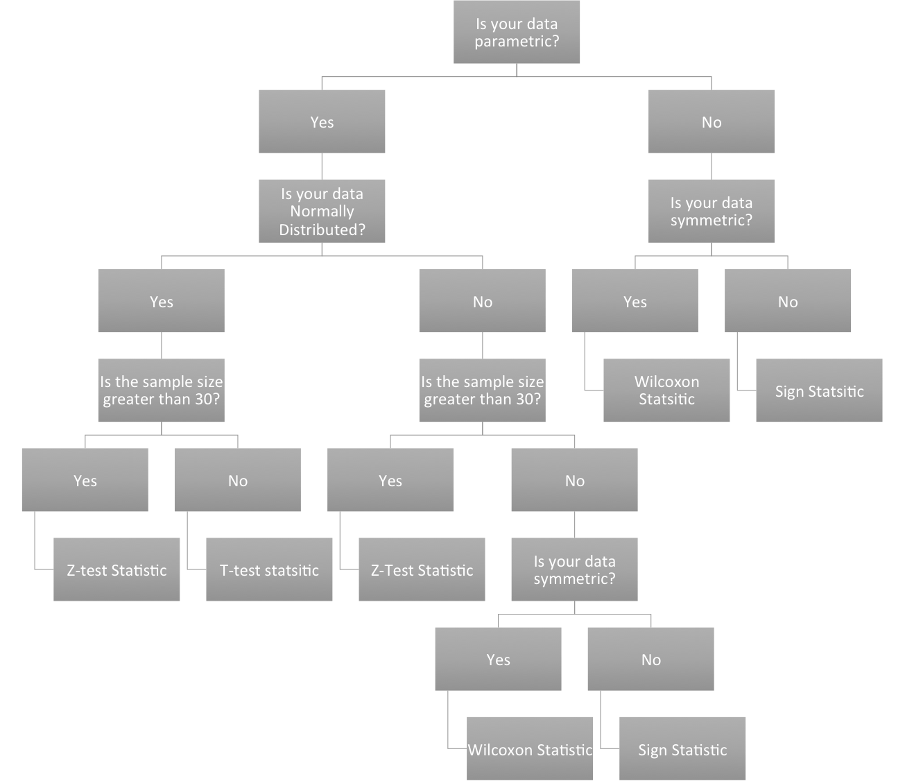
The other popular nonparametric test is the Wilcoxon statistic. This statistic assumes a symmetric distribution - but it can be non-normal. Again, the hypothesis is written in terms of the median (same as above). There are functions in R which I will show later on that will calculate these test statistics for you. Below is another interactive flow chart that shows you one way to pick your test statistic. Again, a static view is available. 

Level of Significance

The next step in the hypothesis testing procedure is to pick a level of significance, alpha (α). Alpha describes the probability that we are rejecting a null hypothesis that is actually true, which is sometimes called a "false positive". Statisticians call this a type I error. We want to minimize this probability of a type I error. To do that, we want to set a relatively small value for alpha, increasing our confidence in the results. You must choose alpha before calculating the test statistics because it determines the threshold of the test statistic beyond which you reject the null hypothesis! The exact value is up to you. Consider the dataset you are using, the problem you are trying to solve, and the amount of confidence you require in your result, or how comfortable you are with the potential of a type I error. The choice depends on the cost, to you, of falsely rejecting the null hypothesis. Two traditional choices for alpha are 0.05 or 0.01, a 5% and 1% probability, respectively, of having a type I error. We would describe this as being 95% or 99% confident in our result.

Since there are type I errors, you're probably not surprised that there are also type II errors. They're just the opposite, falsely not rejecting the null hypothesis, a “false negative”. But this type of error is harder to deal with or minimize. Because of this, we will only focus on the level of significance, alpha. You can read more about type II errors and how to minimize them here.