Prioritize...
After completing this section, you should be able to estimate Z-scores and translate the normal distribution into the standard normal distribution.
Read...
The normal distribution is one of the most common distribution types in natural and social science. Not only does it fit many symmetric datasets, but it is also easy to transform into the standard normal distribution, providing an easy way to analyze datasets in a common, dimensionless framework.
Review of Normal Distribution
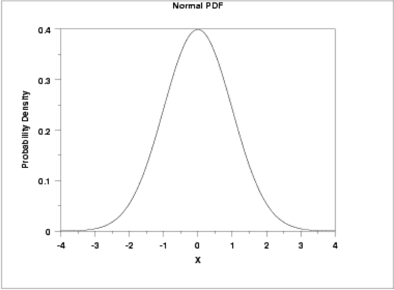
This distribution is parametrized using the mean (μ), which specifies the location of the distribution, and the variance (σ2) of the data, which specifies the spread or shape of the distribution. Some more properties of the normal distribution:
- the mean, median, and mode are equal (located at the center of the distribution);
- the curve is always unimodal (one hump);
- the curve is symmetric around the mean and is continuous;
- the total area under the curve is always 1 or 100%.
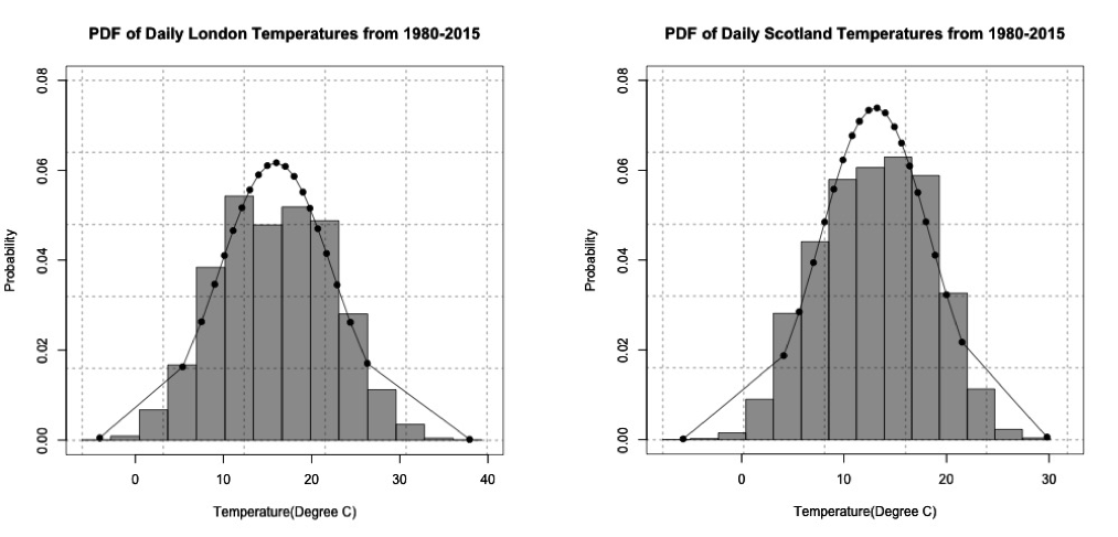
If you remember, temperature was a prime example of meteorological data that fits a normal distribution. For this lesson, we are going to look at one of the problems posed in the motivation. In the video and articles from the newsstand, there was an interesting result: BBQ sales triple when the daily maximum temperature exceeds 20°C in Scotland and 24°C in London. As a side note, there is a spatial discrepancy here: London is a city while Scotland is a country. For this example, I will stick with the terminology used in the motivation (Scotland and London), but I want to highlight that we are really talking about two different spatial regions, and, in reality, this is not what we are comparing because the data is specifically for a station near the city of London and a station near the city of Leuchars, which is in Scotland, but doesn't necessarily represent Scotland as a whole. Let’s take a look at daily temperature in London and Scotland from 1980-2015. Download this dataset. Load the data, and prepare the temperature data by replacing missing values (-9999) with NAs using the following code:
There are two stations: one for London and one for Scotland. Extract out the maximum daily temperature (Tmax) from each station along with the date:
Estimate the normal distribution parameters from the data using the following code:
Finally, estimate the normal distribution using the code below:
The normal distribution looks like a pretty good fit for the temperature data in Scotland and London. The figures below show the probability density histogram of the data (bar plot) overlaid with the distribution fit (dots).
If we wanted to estimate the probability of the Tmax exceeding 20°C in Scotland and 24°C in London, we would first have to estimate the Cumulative Distribution Function (CDF) using the following code:
Remember that the CDF function provides the probability of observing a temperature less than or equal to the value you give it. To estimate the probability of exceeding a particular threshold, you have to take 1-CDF. To estimate the probability of the temperature exceeding a threshold, use the code below:
Since 1980, the temperature has exceeded 20°C in Scotland 9.5% of the time and has exceeded 24°C in London about 10.8% of the time.
Standard Normal Distribution
The simplest case of the normal distribution is when the mean is 0 and the standard deviation is 1. This is called the standard normal distribution, and all normal distributions can be transformed into the standard normal distribution. To transform a normal random variable to a standard normal variable, we use the standard score or Z-score calculated below:
z=x−μσX is any value from your dataset, μ is the mean, σ is the standard deviation, and n is the number of samples. The Z-score tells us how far above or below the mean a value is in terms of the standard deviations. What is the benefit of transforming the normal distribution into the standard normal? Well, there are common tables that allow us to look up the Z-score and instantly know the probability of an event. The most common table comes from the cumulative distribution and gives the probability of an event less than Z. Visually:
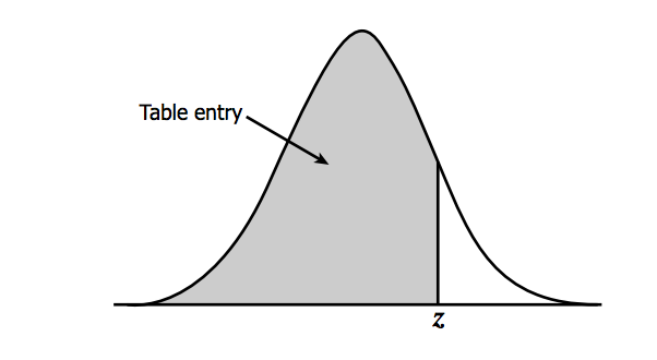
You can find the table here(link is external) and at Wikipedia(link is external) (look under Cumulative). To read the table, take the first two digits of the Z-score and find it along the vertical axis. Then, find the third digit along the horizontal axis. The value where the row and column of your Z-score meets is the probability of observing a Z value less than the one you provided. For example, say I have a Z-score of 1.21, the probability would be .8869. This means that there is an 88.69% chance that my data falls below this Z-score. To translate the temperature data to the standard normal for Scotland and London in R, use the function 'scale' which automatically creates the standardized scores. Fill in the missing code using the variable 'ScotlandTemp':
The standard normal distribution for the temperatures from London and Scotland are shown in the figure below:
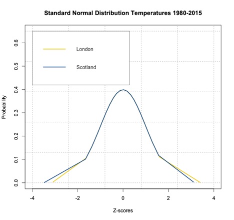
As you can see from the figure, the temperatures have been transformed to Z-scores creating a standard normal distribution with mean 0. If we want to know the probability of temperature falling below a particular value, we can use ‘pnorm’ in R, which calculates the probabilities of any distribution function given its mean and standard deviation. When these two parameters are not provided, ‘pnorm’ calculates the probability for the standard normal distribution function. R thus gives you the choice to transform your normally distributed data into Z-scores. Remember that the Z-scores can be used in the CDF to get a probability of an event with a score less than Z or in the PDF to get the probability density at Z. Fill in the missing spots for the Scotland estimate to compute the probability of the temperature exceeding 20°C.
The probability for the temperature to exceed 20°C in Scotland is about 9.9%, and the probability for the temperature to exceed 24°C in London is about 10.6%, similar to the estimate using the CDF. It might not seem beneficial to translate your results into Z-scores and compute the probability this way, but the Z-scores will be used later on for hypothesis testing.
For some review, try out the tool below that lets you change the mean and standard deviation. On the first tab, you will see Plots: the normal distribution plot and the corresponding standard normal distribution plot. On the second tab (Probability), you will see how we compute the probability (for a given threshold) using the normal distribution CDF and using the Z-table. Notice the subtle differences in the probability values.