Prioritize...
At the end of this section, you should feel confident enough to create and perform your own hypothesis test using parametric methods.
Read...
The best way to learn hypothesis testing is to actually try it out. In this section, you will find two examples of hypothesis testing using the parametric test statistics we discussed previously. I suggest that you work through these problems as you read along. The examples will use the temperature dataset for London and Scotland. If you haven’t already downloaded it, I suggest you do that now. Each example will work off of the previous example, and the complexity of the problem will increase. However, for each example, I will pose a question and then work through the following procedure which was discussed previously step by step. You should be able to easily follow along.
- State the question.
- Select the null and alternative hypothesis.
- Check basic assumptions.
- Identify the test statistic.
- Specify the level of significance.
- State the decision rules.
- Compute the test statistics and calculate confidence interval.
- Make decision about rejecting null hypothesis and interpret results.
Z-Statistic Two Tailed
- State the Question
If you remember from the motivation, I highlighted a video that showcased an interesting relationship between BBQ sales and temperature in London and Scotland. If the temperature exceeds a certain threshold (from here on out I will call this the BBQ temperature threshold), 20°C for Scotland and 24°C for London, BBQ sales triple. Here is my question:Is the BBQ temperature threshold in Scotland and London a temperature that is typically observed in summer?My instinct is that the BBQ temperature threshold is not what is generally observed in London and Scotland during the summer and that’s why the BBQ sales triple; it's an ‘unusual’ temperature that spurs people to go out and buy or make BBQ. To assess this question, I'm going to use the daily temperature dataset from London and Scotland from 1980-2015 subsampled for the summer months (June, July, and August). Here is the code to subsample for summer:
Show me the code... - Select the null and alternative hypothesis
Since my data is parametric, I will state my hypothesis with respect to the mean (μ) instead of the median (η). My instinct is that the BBQ temperature threshold does not equal the mean temperature observed in London and Scotland during the summer months. The null hypothesis will therefore be stated as the opposite; that is that the BBQ temperature threshold is equal to the mean temperature.Ho:μ=20 (Scotland) Ho:μ=24 (London) This is a two sided test. We will assume that the mean temperature is equal to the BBQ temperature threshold, so we will test whether the mean temperature lies above or below. If it does, then we reject the null hypothesis. The alternative hypothesis will be:
H1:μ≠20 (Scotland)H1:μ≠24 (London) - Check basic assumptions
We need to determine what type of data I have and whether it's usable for hypothesis testing. The data is independent and randomly sampled. In addition, I previously showed that this temperature dataset is normally distributed. This means that my data is parametric (fits a normal distribution), and, therefore, I can continue on with the hypothesis testing. - Identify the test statistic
Since the data is normally distributed, we can use a Z-test or a t-test. The dataset is quite large, even with the subsampling for summer months (more than 1000 samples), so we can safely use the two-sided Z-test. - Specify the level of significance
We have a very large dataset, so I feel comfortable making the level of significance very small, thereby minimizing the potential of type I errors. I will set the level of significance (α) to 0.01. - State the decision rules
I generally prefer the P-value approach, but I will show the Critical Value approach for this one example. Let’s first visualize the two sided rejection region:If the P-value is less than 0.005 (α/2) or the Z-score is less then -2.58 (-Zα/2) or greater than 2.58 (Zα/2), we will reject the null hypothesis: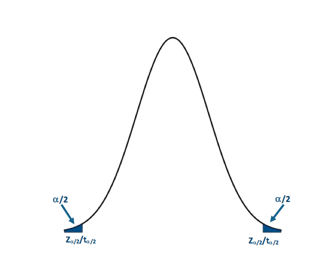 Visual of the two-sided test.Credit: J. Roman
P-value<0.005 Z-score<−2.58 or Z-score>2.58 - Compute the test statistics and calculate confidence interval
Now we can calculate the test statistic along with the confidence interval for the mean of the dataset. I will use the function 'z.test' in R to compute my Z-test. Here is the code to compute the Z-score:Show me the code...You will notice that I've assigned 'alternative' to "two.sided", so the function performs a two sided test. I set the confidence level to 0.99. This means that my confidence interval for the mean summer temperature will be at the 99% level. The P-value for the London test is 2.2e-16 and the Z-score is -19.978. The confidence interval is (22.36067°C, 22.73512°C). For Scotland, the P-value is 2.2e-16 and the Z-score is -27.712. The confidence interval is (18.27994°C, 18.57251°C). - Make decision about rejecting null hypothesis and interpret results
Remember our decision rule to reject the null hypothesis:
P-value<0.005 Z-score<−2.58 or Z-score>2.58 For both London and Scotland, our P-values and Z-scores are less than the critical values, so we can confidently reject the null hypothesis in favor of the alternative hypothesis. This means that the BBQ temperature threshold does not equal the summer time mean temperature observed in each city with a 1% probability of a type I error. We are 99% confident that the mean summer temperature is within the range of 22.36°C and 22.74°C for London and 18.28°C and 18.57°C for Scotland, about 2°C less than the BBQ temperature threshold values. This hints that the temperature threshold for BBQ sales is warmer than the average summer temperature, and has a smaller probability of occurring. There are fewer chances for BBQ retailers to utilize this relationship and maximize potential profits through marketing schemes.
T-Statistic One Tailed
The technological world we live in allows us to instantaneously ‘Google’ something we don't know. For example, where is a good BBQ place? What’s the best recipe for BBQ chicken? What BBQ sauce should I use for my ribs? Google Trends is an interesting way to gain insight into what is trending. Below is a figure showing the interest in 'BBQ' over time in London based on the number of queries Google received:
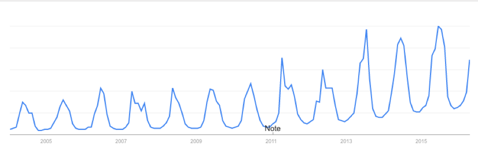
You will notice that the interest varies seasonally, which is expected, and each year there is a peak. June 2015 saw the most queries of the word 'BBQ' in London. I see two possible reasons for the large query in June. The first is that the temperature in June 2015 was relatively warm and the BBQ temperature threshold was met quite often, resulting in a large number of BBQ queries for the month. The second is that the temperature in June 2015 was actually quite cool and the BBQ temperature threshold was rarely met. When it was, more people were interested in getting out and either grilling or getting some BBQ. During a cold stretch, I personally look forward to that warm day. I make sure I’m outside enjoying the rare warm weather. My inclination is that during June 2015 the mean temperature for the month was cooler than the BBQ temperature threshold. So once that threshold was met, a spur of 'BBQ' inquiries occurred.
- State the Question
Was the mean temperature in June of 2015 less than the BBQ temperature threshold?
To answer this question, I'm going to use daily temperatures from June 1st 2015-June 30th 2015 for London and Scotland. First, we have to extract the temperatures for this time period. Use the code below:
Show me the code... - Select the null and alternative hypothesis
Since my data is parametric, I will state my hypothesis with respect to the mean (μ) instead of the median (η). The instinct is that the mean temperature in June 2015 was cooler than the BBQ temperature threshold. The null hypothesis will be stated as the opposite of my instinct: that is, that the mean temperature in June was warmer than the BBQ temperature threshold. Ho:μ≥20 (Scotland) Ho:μ≥24 (London) This is a lower one-tailed test. We will assume that the mean temperature is greater than the threshold, so we will test if the mean temperature lies in the region below or less than the BBQ temperature threshold. If it does, then we reject the null hypothesis and accept the alternative hypothesis which is: H 1 :< - Check basic assumptions
Again, we know that temperature is normally distributed and the data is independent and random, so we can continue with the hypothesis testing. - Identify the test statistic
Since the data is normally distributed, we can use a Z-test or a t-test. The dataset has been sub-sampled, however, and the number of samples is no more than 30. We must use the lower one-tailed t-test. - Specify the level of significance
Since we have a smaller dataset, I'm going to set the significance level (α) to 0.05. I still want to minimize the potential of type I errors but, because of the small sample size, I will loosen the constraint on type I errors. - State the decision rules
I'm only going to use the P-value approach for this example. Let's visualize the lower one-sided rejection region:If the P-value is less than 0.05 (α), we will reject the null hypothesis in favor of the alternative: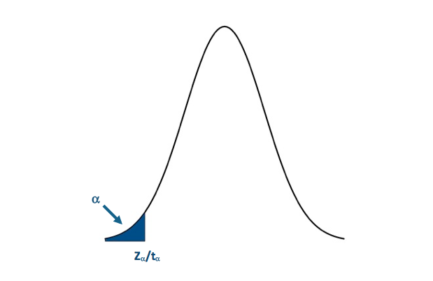 Visual of the lower one-sided test.Credit: J. Roman
- Compute the test statistics and calculate confidence interval
Now we can calculate the test statistic along with the confidence interval for mean temperature in June 2015. I will use the function 't.test' in R to compute my t-test. The code is supplied for London. Fill in the missing parts for Scotland: You will notice that I've assigned 'alternative' to "less" so the function performs a lower one-tailed test. I set the confidence level to 0.95. This means that my confidence interval will be at the 95% level. The P-value for the London test is 0.002735. The confidence interval is (-Inf, 23.19994ºC). Remember that for one-tailed tests, we only create an upper or lower bound for the interval (depending on the type of test). For Scotland, the P-value is 0.0001958. The confidence interval is (-Inf,18.53317ºC). - Make decision about rejecting null hypothesis and interpret results
Remember our decision rule to reject the null hypothesis was:
For both London and Scotland, our P-value is less than the critical P-value so we can confidently reject the null hypothesis in favor of the alternative hypothesis. The population mean for June temperatures in 2015 was less than the BBQ temperature threshold in each location with a 5% probability of a type I error.