Empirical Rule and Central Limit Theory

Read...

The extensive use of the normal distribution and the easy transformation to the standard normal distribution has led to the development of common guidelines that can be applied to this PDF. Furthermore, the central limit theory allows us to invoke the normal distribution, and the corresponding rules, on many common datasets.

Empirical Rule

The empirical rule, also called the 68-95-99.7 rule or the three-sigma rule, is a statistical rule for the normal distribution which describes where the data falls within three standard deviations of the mean. Mathematically, the rule can be written as follows:

$$P\left(\mu -\sigma \le x\le \mu +\sigma \right)\approx 0.683$$ $$P\left(\mu -2\sigma \le x\le \mu +2\sigma \right)\approx 0.955$$ $$P\left(\mu -3\sigma \le x\le \mu +3\sigma \right)\approx 0.997$$

The figure below shows this rule visually: 

Figure showing that 99.7% of the data are within 3 standard deviations of the mean, 95% is within 2 standard deviations, and 68% is within 1 standard deviation.

Credit: Dan Kernler (Own work) [CC BY-SA 4.0], via Wikimedia Commons

What does this mean exactly? If your data is normally distributed, then typically 68% of the values lie within one standard deviation of the mean, 95% of the values lie within two values of the mean, and 99.7% of your data will lie within three standard deviations of the mean. Remember the Z-score? It defines how many standard deviations you are from the mean. Therefore, the empirical rule can be described in terms of Z-scores. The number in front of the standard deviation (1, 2, or 3) is the corresponding Z number. The figure above can be transformed into the following:

Example of the three-sigma score with the Z-scores listed.

Credit: J. Roman edits of Dan Kernler (Own work) [CC BY-SA 4.0], via Wikimedia Commons

This rule is multi-faceted. It can be used to test whether a dataset is normally distributed and checks whether the data lies within 3 standard deviations. The rule can also be used to describe the probability of an event outside a given range of deviations, or used to describe an extreme event. Check out these two ads from Buckley Insurance and Bangkok Insurance.

Both promote insuring against extreme or unlikely weather events (outside the normal range) because of the high potential for damage. So, even though it is unlikely that you will encounter the event, these insurance companies use the potential of costly damages as a motivator to buy insurance for rare events.

The table below, which expands on the graph above, shows the range around the mean, the Z-score, the area under the curve over this range (the probability of an event in this range), the approximate frequency outside the range (the likelihood of an event outside the range), and the corresponding frequency to a daily event outside this range (if you are considering daily data, translate the frequency into a descriptive temporal format).

A word of caution: the descriptive terminology in the table (twice a week, yearly, etc.) can be controversial. For example, you might have heard the term 100-year flood (for example the 2013 floods in Boulder, CO). The 100-year flood has a 1 in 100 (1%) chance of occurring every year. But how do you actually decide what the 100-year flood is?  When you begin to exceed a frequency greater than the number of years in your dataset, this interpretation becomes foggy. If you do not have 100 years of data, claiming an event occurs every 100 years is more of an inference of the statistics than an actual fact. It’s okay to make inferences from statistics, and this can be quite beneficial, but make sure that you convey the uncertainty. Furthermore, people can get confused by the terminology. For example, when the 100-year flood terminology was used in the Boulder, CO floods, many thought that it was an event that occurs once every 100 years, which is incorrect. The real interpretation is: the event had a 1% chance of occurring each year. Here is an interesting article on the 100-year flood in Boulder, CO and the use of the terminology.

Central Limit Theorem

At this point, everything we have discussed is based on the assumption that the data is normally distributed. But, what if we have something other than a normal distribution? There are equivalent methods for other parametric distributions that we can use, but let's first discuss a very convenient theory called the central limit theorem. The central limit theorem, along with the law of large numbers, are two theorems fundamental to the concept of probability. The central limit theorem states:

The sampling distribution of the mean of any independent random variable will be approximately normal if the sample size is large enough, regardless of the underlying distribution. 

What is a sampling distribution of the mean? Consider any population. From that population, you take 30 random samples. Estimate the mean of these 30 samples. Then take another 30 random samples and estimate the mean again. Do this again and again and again. If you create a histogram of these means, you are representing the sampling distribution of the mean. The central limit theorem then says that if your sample size is large enough, this distribution is approximately normal. 

Let’s work through an example using the precipitation data from Lesson 1. As a reminder, this data was daily precipitation totals from the Amazon. You can find the dataset here. Load the data in and extract out the precipitation:

# load in precipitation data 
mydata2 <- read.csv("daily_precipitation_data_AmazonBrazil.csv", header=TRUE, sep=",")

# extract out precipitation (convert from tenths of a mm to mm)
precip <- mydata2$PRCP/10 

# replace data with bad quality flags with NA 
precip[which(mydata2$Quality.Flag != "")] <- NA

We found that the Weibull distribution was the best fit for the data. The figure below is the probability density histogram of the precipitation data with the Weibull estimate overlaid.

Probability density histogram of daily precipitation for the Amazon. The blue line is the estimation of the weibull distribution.

Credit: J. Roman

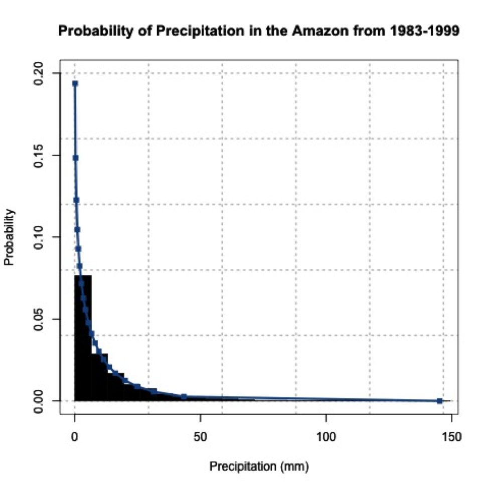
When you look at the figure, you can clearly tell it looks nothing like a normal distribution! Let’s put the central limit theory to the test. We need to first create sample means from this dataset. Since the underlying distribution is Weibull, we will need quite a few sample mean estimates to converge to a normal distribution. Let’s estimate 100 sample means randomly from the dataset. We have 6195 samples of daily precipitation in the dataset, but only 3271 are greater than 0 (we will exclude values of 0 because we are interested in the mean precipitation when precipitation occurs). Use the code below to remove precipitation equal to 0.

# replace precipitation =0 with NA
precip[which(precip == 0)] <- NA

# omit NA
good_precip <- na.omit(precip)

For each sample mean, let's use 30 data points. We will randomly select 30 data points from the dataset and compute the sample mean 100 times. To do this, we will use the function 'sample' which randomly selects integers over a range. Run the code below (no need to fill anything in), and look at the histogram produced. 

We provided 'sample', a range from 1 through the number of data points we have. Thirty is the number of random integers we want. Setting replace to 'F' means we won’t get the same numbers twice.

You can see that the histogram looks symmetric and resembles a normal distribution. If you increased the number of sample mean estimates to 1000, you would get the following probability density histogram:

Probability density histogram of the 1000 calculated sample means of daily precipitation for the Amazon. The blue line is the fitted normal distribution.

Credit: J. Roman

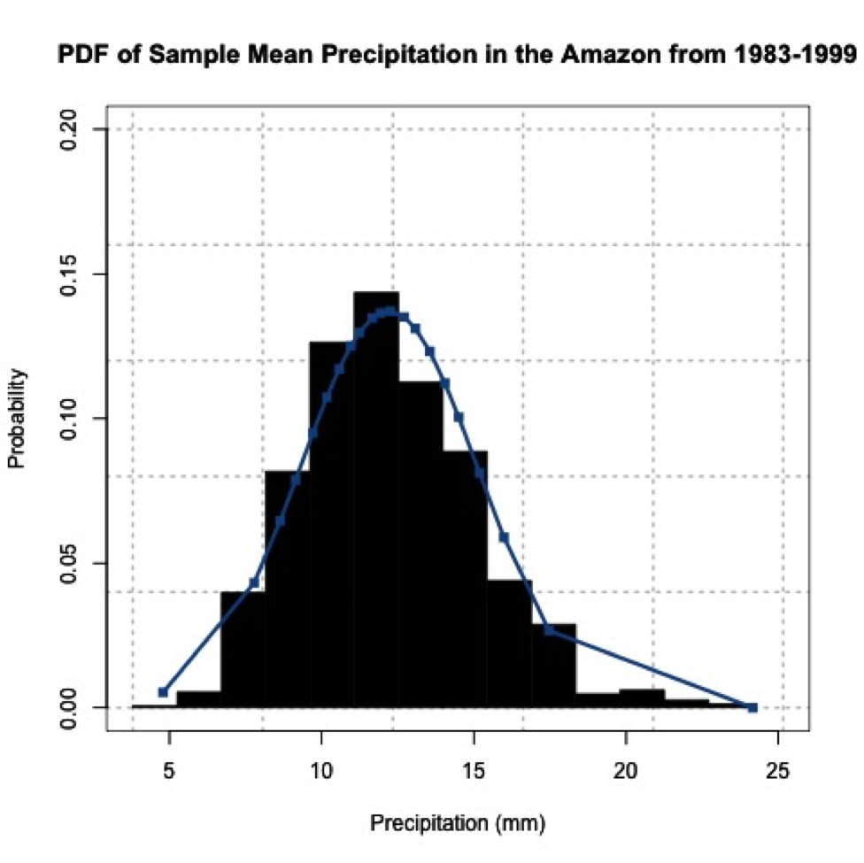
The more sample means, the closer the histogram looks to a normal distribution. One thing to note, your figures will not look exactly the same as mine and if you rerun your code you will get a slightly different figure each time. This is because of the random number generator. Each time a new set of indices are created to estimate the sample means, thus changing your results. We will, however, still get a normally distributed dataset; proving the central limit theory and allowing you to assume that any independent dataset of sample means will converge to a normal distribution if the sample size is large enough.