Prioritize...
At the end of this section, you should feel confident enough to create and perform your own nonparametric hypothesis test.
Read...
In this section, you will find two examples of hypothesis testing using the nonparametric test statistics we discussed previously. Again, I suggest that you work through these problems as you read along. The examples will use the temperature dataset for London and Scotland. Each example will work off of the previous example and the complexity of the problem will increase. For each example, I will again pose a question and then work through the procedure discussed previously step by step. You should be able to easily follow along.
- State the question.
- Select the null and alternative hypothesis.
- Check basic assumptions.
- Identify the test statistic.
- Specify the level of significance.
- State the decision rules.
- Compute the test statistics and calculate confidence interval.
- Make decision about rejecting null hypothesis and interpret results.
Wilcoxon One Tailed
Ads are not only displayed in the newspaper anymore; they are seen online, through apps on your phone or tablet, and can be constantly updated or changed. Although new platforms for advertising may seem beneficial, the timing of an ad is everything. Check out this marketing strategy by Pantene:
Depending on the weather conditions, an ad will appear that promotes a specific type of shampoo/conditioner that will counteract those conditions. The ad is time and location dependent; only displaying at the most advantageous time for a particular location.
From a marketing perspective, it would be advantageous to display ads for BBQ when people are most interested in BBQ. Since BBQ sales triple when the temperature reaches a particular threshold, we can use that information as a guideline for choosing the optimal advertising time. We should also take advantage of the time when people are querying for BBQ; online advertisement is a great way to market to thousands of people. So, how does the inquiry of BBQ relate to the BBQ temperature threshold? We can determine which week in a given year London and Scotland are most likely to observe temperatures above the BBQ temperature thresholds. But do the inquiries on BBQ peak during the same week?
- State the question
Does the peak week in BBQ inquiries coincide with the week in which the BBQ temperature threshold is most likely to occur?
To answer this question, I'm going to extract every date in which the temperature exceeded the BBQ temperature threshold for London and Scotland. Instead of working with day/month/year, I will work with ‘weeks'. That is what week (1-52) can we expect the temperature to exceed the BBQ threshold. Use the code below to extract out the dates and transform them into weeks:
Show me the code...The variable ScotlandBBQWeeks and LondonBBQWeeks represents every instance from 1980-2015 in which the temperature reached or was above the required BBQ threshold in the form of weeks (1-52). The range is between week 13 and week 42.
- Select the null and alternative hypothesis
Since I'm conducting a nonparametric test, I will state my hypothesis with respect to the median (η) instead of the mean (μ). My instinct is that the most likely week in which the temperature will be above the BBQ temperature threshold occurs after the week of peak BBQ inquiries. The peak week of BBQ inquiries through Google trends is week 22 for both London and Scotland. This was computed by calculating the median peak week based on the 12 years of Google trend data available. The null hypothesis will be stated as the opposite.
Ho:η≤22 (Scotland)Ho:η≤22 (London)This is an upper one-tailed test. We will assume that the BBQ temperature threshold week is before the peak inquiry week, so we will test if the BBQ temperature threshold week lies in the region above the inquiry week. If it does, then we reject the null hypothesis, and accept the alternative hypothesis, which is: H1:η>22 (Scotland)H1:η>22 (London) - Check basic assumptions
Now temperature is normally distributed, but I'm not examining temperature in this case. I'm looking at weeks. Look at the histograms for the ScotlandBBQWeeks and the LondonBBQWeeks:I'm not going to assume that it does not fit any particular distribution. That is, I'm going to conduct a nonparametric test.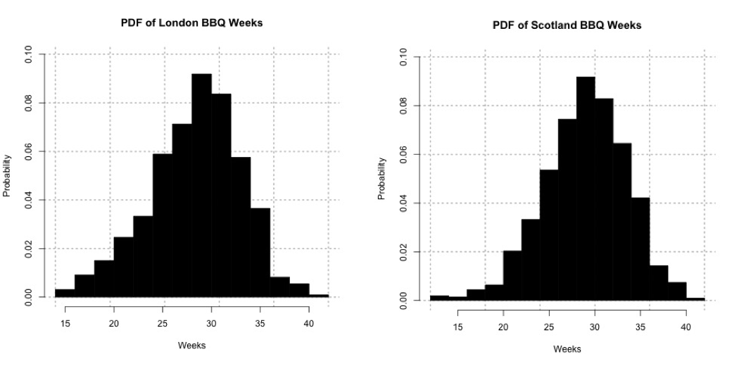 Probability density histogram of weeks in which the temperature is greater than or equal to 24oC for London (left) and 20oC Scotland (right).Credit: J. Roman
 - Identify the test statistic
We are using a nonparametric test static. The data appears somewhat symmetric so I will use the Wilcoxon test statistic. - Specify the level of significance
Since we have a fairly large sampling (more than 100 samples), I'm going to set the significance level (α) to 0.01. - State the decision rules
I'm only going to use the P-value approach for this example. Let's visualize the upper one-tailed rejection region:If the P-value is less than 0.01 (α) we will reject the null hypothesis in favor of the alternative.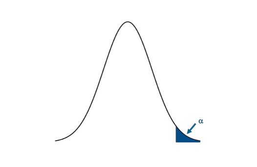 Visual of the upper one-sided test.Credit: J. Roman
P-value<0.01 - Compute the test statistics and calculate confidence interval
Now we can calculate the test statistic along with the confidence interval for the median week in which the temperature exceeds the BBQ temperature threshold. I will use the function ‘wilcox.test' in R to compute my nonparametric test statistic. Here is the code for London, fill in the missing parts for Scotland: You will notice that I've assigned 'alternative' to "greater" so the function performs an upper one-tailed test. I also had to use the command 'as.numeric'; this translates the strings in the variable “Scotland/LondonBBQWeeks” into integers. I set the confidence level to 0.99. This means that my confidence interval will be at the 99% level. The P-value for the London test is 2.2e-16. The confidence interval is (28.99999th week Inf). Remember that for one-tailed tests, we only create an upper or lower bound for the interval (depending on the type of test). For Scotland, the P-value is 2.2e-16. The confidence interval is (29.49995th week, Inf). - Make decision about rejecting null hypothesis and interpret results
Remember our decision rule to reject the null hypothesis:
P-value<0.01For both London and Scotland, our P-value is less than the critical P-value, so we confidently reject the null hypothesis in favor of the alternative hypothesis. The week in which the temperature is most likely to exceed the BBQ threshold is after the week of peak Google inquiries, with a 1% chance of having a type I error. We are 99% confident that the week for exceeding the BBQ temperature threshold is at least the 29th week for London and the 30th week for Scotland, more than 6 weeks after the peak inquiry week. This result suggests that people are inquiring way before they are most likely to observe a temperature above the BBQ threshold. Remember that the BBQ temperature threshold is the temperature in which BBQ sales triple. So why is there this disconnect? Maybe people are relying on a forecast? But a 6-week forecast is generally not reliable. Or maybe the inquiry actually occurs when we first reach the BBQ temperature threshold; after that initial event and inquiry we know everything about BBQ so we don't need to Google it again.
Sign Test Two Tailed
A natural follow-on question would be: does the peak inquiry week coincide with the first week in which we observe temperatures above the BBQ temperature threshold? This would be an optimal time to advertise for BBQ products online.
- State the question
Does the peak week in BBQ inquiries coincide with the first week in which the temperature exceeds the BBQ threshold?
To answer this question, I'm going to extract the first week each year in which the temperature exceeds the BBQ threshold for London and Scotland. Use the code below to extract out the dates and transform the dates into weeks:
Show me the code... - Select the null and alternative hypothesis
Since my data is nonparametric, I will state my hypothesis with respect to the median (η) instead of the mean (μ). The null hypothesis will be that the peak week of inquiries coincides exactly with the typical first week of temperatures exceeding the BBQ threshold: Ho:η=22 (Scotland)Ho:η=22 (London)This is a two tailed test. We will assume that the first week coincides with the peak inquiry week, so we will test if the first week lies above or below the inquiry week. If it does, then we reject the null hypothesis, and accept the alternative hypothesis which is: H1:η≠22 (Scotland)H1:η≠22 (London) - Check basic assumptions
Again, I will be examining ‘weeks' instead of temperature. Look at the histograms for the FirstScotlandBBQWeek and the FirstLondonBBQWeek, which is the week in which we first observe temperatures above the BBQ temperature threshold:The data for Scotland definitely does not fit a parametric distribution, so I will continue on with the nonparametric process.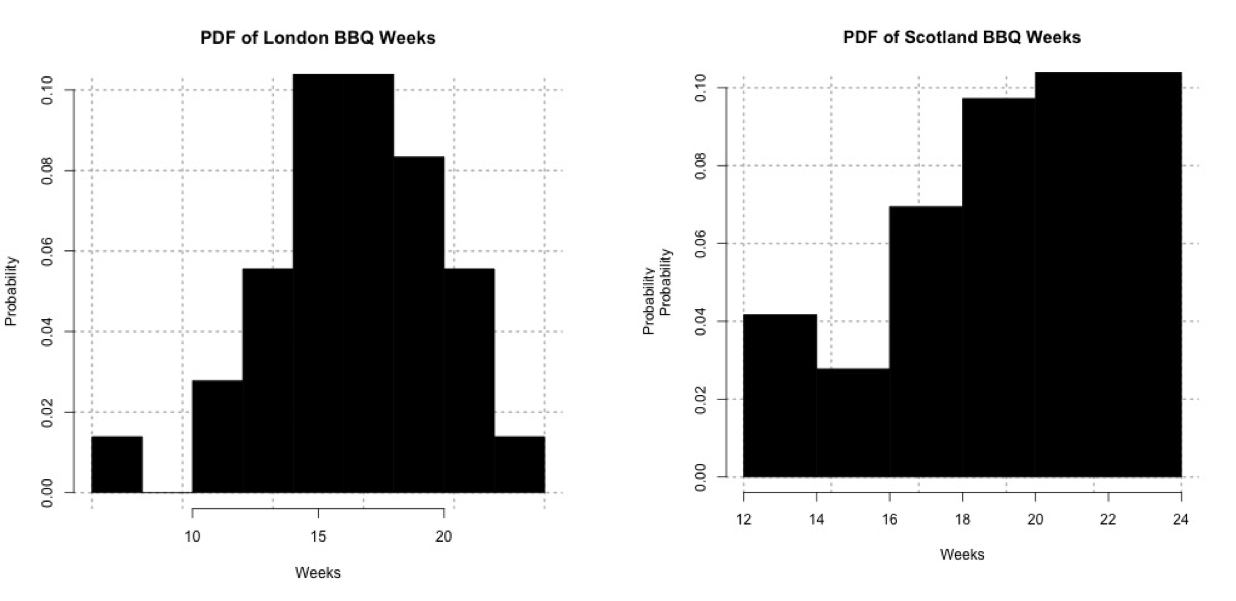 Probability histogram of the first week in which the temperature exceeds 24oC for London (left) and 20oC for Scotland (right).Credit: J. Roman
 - Identify the test statistic
Since the data is nonparametric we need to use a nonparametric test statistic. The data doesn't appear very symmetric, especially for Scotland, so I will use the Sign test. - Specify the level of significance
We have one week for each year, so that's 36 samples total. This is fairly small, so I will loosen the constraint on the level of significance. I'm going to set the significance level (α) to 0.05. - State the decision rules
I'm only going to use the P-value approach for this example. Let's visualize the two-tailed rejection region:If the P-value is less than 0.025 (α/2), we will reject the null hypothesis in favor of the alternative.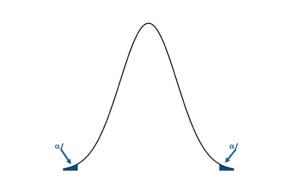 Visual of the two-sided test.Credit: J. Roman
P-value<0.025 - Compute the test statistics and calculate confidence interval
Now we can calculate the test statistic along with the confidence interval for the range in which we expect to first observe the temperature exceeding the BBQ threshold. I will use the function 'SIGN.test' in R to compute my nonparametric test statistic. Here is the code:Show me the code...You will notice that I've assigned 'alternative' to "two.sided" so the function performs a two-sided test. I also have to use the command 'as.numeric'; this translates the strings into integers. I set the confidence level to 0.95. This means that my confidence interval will be at the 95% level. The P-value for the London test is 4.075e-09. The confidence interval is (16th week, 18th week). For Scotland, the P-value is 0.02431. The confidence interval is (19th week, 21.4185st week). - Make decision about rejecting null hypothesis and interpret results
Remember our decision rule to reject the null hypothesis:P-value<0.025For London and Scotland, our P-value is less than the critical P-value. We can confidently reject the null hypothesis in favor of the alternative hypothesis. The first week in which we exceed the temperature threshold for BBQ sales does not coincide with the week of peak inquiries, with a 5% chance of creating a type I error. For London, the first week in which we exceed the temperature threshold is most likely to occur between the 16th week and the 18th week, with a 95% confidence level. For Scotland, the first week in which we are most likely to exceed the temperature threshold occurs between the 19th and 21st week, at a 95% confidence level. In terms of supply and demand for a retailer, a store might consider increasing their BBQ supplies during these weeks. In terms of marketing, for London, the peak inquiry occurs more than a month after the first occurrence of temperature above the BBQ threshold, while for Scotland it is less than a week; highlighting the need for advertising that is both time and location relevant. In-store ads would potentially be more successful coinciding when the temperature exceeds the BBQ threshold and customers are known to buy more products. If, however, you want to catch the BBQ inquiry at its peak, you might display online ads a week (3 weeks) after the first occurrence of temperature exceeding the BBQ threshold in Scotland (London) to get a better impact online and possibly invoke a second wave of BBQ sales.